Article

Impact of Climate and Land Cover Dynamics on River Discharge in the Klambu Dam Catchment, Indonesia

by
Fahrudin Hanafi
1,
Lina Adi Wijayanti
1,
Muhammad Fauzan Ramadhan
1,
Dwi Priakusuma
1 and
Katarzyna Kubiak-Wójcicka
2,*
1
Faculty of Social and Political Sciences, Universitas Negeri Semarang, Gunungpati, Semarang 50229, Indonesia
2
Faculty of Earth Sciences and Spatial Management, Nicolaus Copernicus University, Gagarina 11, 87-100 Toruń, Poland
*
Author to whom correspondence should be addressed.
Water 2026, 18(2), 250; https://doi.org/10.3390/w18020250 (registering DOI)
Submission received: 22 December 2025 / Revised: 10 January 2026 / Accepted: 13 January 2026 / Published: 17 January 2026
(This article belongs to the Special Issue Water Management and Geohazard Mitigation in a Changing Climate)

Abstract

This study examines the hydrological response of the Klambu Dam Catchment in Central Java, Indonesia, to climatic and land cover changes from 2000–2023, with simulations extending to 2040. Utilizing CHIRPS satellite data calibrated with six ground stations, monthly precipitation and temperature datasets were analyzed and projected via linear regression aligned with IPCC scenarios, revealing a marginal temperature decline of 0.21 °C (from 28.25 °C in 2005 to 28.04 °C in 2023) and a 17% increase in rainfall variability. Land cover assessments from Landsat imagery highlighted drastic changes: a 73.8% reduction in forest area and a 467.8% increase in mixed farming areas, alongside moderate fluctuations in paddy fields and settlements. The Thornthwaite-Mather water balance method simulated monthly discharge, validated against observed data with Pearson correlations ranging from 0.5729 (2020) to 0.9439 (2015). Future projections using Cellular Automata-Markov modeling indicated stable volumetric flow but a temporal shift, including a 28.1% decrease in April rainfall from 2000 to 2040, contracting the wet season and extending dry spells. These shifts pose significant threats to agricultural and aquaculture activities, potentially exacerbating water scarcity and economic losses. The findings emphasize integrating dynamic land cover data, climate projections, and empirical runoff corrections for climate-resilient watershed management.

1. Introduction

Water resources depend on many factors, both natural, primarily climatic, and anthropogenic. Of these climatic factors, precipitation and air temperature primarily influence the volume of water resources [1,2]. In addition to climatic conditions, the volume and variability of water resources are influenced by the physiographic characteristics of the river basin, such as soil permeability, topography, land use, and human activity. Despite numerous studies on the spatiotemporal variability of water resources due to climate change, changes resulting from rapid economic development are increasingly documented. Rapid economic development, combined with population growth, is driving rapid urbanization and changes in land use [3]. Human overexploitation of the natural environment, including urban expansion, leads to deforestation and the growth of urbanized areas, which in turn causes changes in the ecosystem structure. Changes in land use and LULC have significant impacts on atmospheric components such as precipitation and temperature, key drivers of the hydrological cycle [4,5,6]. Consequently, the natural hydrological cycle is disrupted, affecting key processes including infiltration rates, groundwater recharge mechanisms, evaporation and transpiration patterns, and surface runoff generation [7,8,9].
Land-use and land cover (LU/LC) changes vary globally, with deforestation and urbanization accelerating runoff in regions like the Amazon Basin [10] and Mekong River [11], while reforestation mitigates it in areas such as China’s Loess Plateau [12]. These alterations reduce evapotranspiration and enhance surface flow, amplifying hydrological responses to climate change, as seen in differential impacts across catchments due to local conditions like soil and topography [13,14]. For example, LU/LC-driven runoff increases exacerbate floods in humid watersheds like Australia’s Murray-Darling Basin [15] and droughts in arid ones like Europe’s rivers [16]. Models such as SWAT and VIC confirm that deforestation can boost runoff by 10–20% [10], underscoring the need for catchment-scale assessments to inform sustainable water management [17,18].
The rate of land-use change varies across regions [19,20,21,22]. Local hydrological conditions vary across locations, leading to differential impacts of climate change on both hydrological processes and ecosystem dynamics, even under identical climate projections [23,24]. Therefore, accurate assessment of water flow at the catchment scale has become essential for developing a framework for sustainable water allocation and implementing effective management strategies.
Indonesia exemplifies the complex water resource challenges faced by people living in monsoon-dominated regions. Indonesia is the largest country in Southeast Asia by area and one of the four most populous countries in the world. In recent years, Indonesia has experienced steady population growth, and the country has recently faced significant water scarcity problems [25]. In 2023, Indonesia had an estimated 280 million inhabitants, with further population growth expected in subsequent years [26]. Furthermore, Indonesia’s unique geography, including its archipelago and diverse landscape, combined with the monsoon season, leads to cyclical water abundance and scarcity [27].
River basins in Indonesia are experiencing increasing pressure from the effects of climate change, accelerated urbanization, and intensive agricultural and industrial development. Despite existing infrastructure, including river hydrotechnical development, which consists of reservoirs serving various functions (water supply, electricity generation, irrigation), river basins currently face numerous challenges that threaten their hydrological sustainability [28,29]. For example, river basins in Java Island play a key role in regional water security, particularly in terms of sustainable agriculture and reliable urban water supply.
Recent hydrological evaluations suggest that Java is anticipated to confront acute water shortages, characterized by significant fluctuations in seasonal water availability that impact both surface water and groundwater supplies [30]. The swift alteration of land use patterns, in conjunction with climatic variability, has resulted in heightened runoff and diminished baseflow contributions to annual streamflow, thereby fundamentally transforming watershed hydrology. This phenomenon raises considerable concerns for agricultural areas reliant on irrigation systems [31]. Within the context of Java, research has revealed that alterations in precipitation patterns and temperature dynamics are exacerbating the frequency and intensity (shifting) [32] of extreme hydrological occurrences, thereby influencing both the quantity of water available and its temporal distribution. The complexity of the situation is further aggravated by escalating demands for water and diminishing discharge rates in critical watersheds at Java regions [33], particularly during arid seasons. These alterations present substantial challenges to the management of water infrastructure, as conventional operational frameworks may become misaligned with the shifting hydrological dynamics.
Investigations have indicated that watersheds in Java are undergoing rapid transformations in their hydrological characteristics, thereby necessitating the implementation of adaptive management strategies and improved monitoring frameworks. This intricate interaction between climate change, water resource dynamics, and infrastructure management necessitates a more sophisticated comprehension of watershed responses to environmental transformations, particularly in vital agricultural areas where water security has direct implications for food production [34] and socioeconomic viability.
Land cover changes significantly influence watershed management, especially in critical areas like Klambu Dam, part of the Serang River Basin in Central Java. Based on data from the Central Bureau of Statistics (BPS), between 2000 and 2020, significant land cover transformations were observed across Central Java, with forest areas declining by approximately 25%, while agricultural land expanded by around 15%. In the Babon River watershed, similar trends have been observed, where the conversion of forest and shrubland into paddy fields and urban areas has intensified surface runoff, reduced soil infiltration, and contributed to higher sediment loads in water bodies [35]. These shifts in land cover affect the hydrological cycle by increasing peak flows during rainy seasons and reducing baseflow during dry periods, making it challenging to maintain water resource stability at Klambu Dam.
Land cover data is crucial in water resource planning. The utilization of medium-scale imagery such as Landsat series greatly facilitates the regular identification and monitoring of land cover data. Moreover, with recent advancements, land cover can be modeled for future scenarios using Cellular Automata [36], as demonstrated through the Markov Chain approach or Artificial Neural Networks (ANN) [37]. This enables planners to anticipate changes in land cover patterns, providing valuable insights for sustainable watershed management and water resource allocation in the future [38].
Effective watershed management in this context must incorporate land cover data and hydrological models to predict and mitigate the impacts of these changes. For example, the decline in vegetative cover has been linked to increased erosion rates and sediment deposition in water channels, reducing the storage capacity of reservoirs and impacting irrigation and flood control [39]. By integrating remote sensing data and field measurements, strategies such as reforestation, soil conservation practices, and sustainable land use planning are essential to enhance water quality [39] and improve the resilience of Klambu Dam against the effects of climate variability and land degradation. A critical research gap exists regarding the integration of land cover changes, climate variability, and river discharge dynamics in tropical regions of Indonesia. Previous studies have predominantly focused on a singular aspect, either analyzing land cover change, examining climate variability, or assessing hydrological responses. This fragmented approach limits the ability to comprehensively understand the interactions between these components, which are crucial for sustainable watershed management. This study addresses this gap by employing a comprehensive and integrated methodology. The Thornthwaite-Mather method is applied to assess river discharge, while future land use projections are modelled using the Cellular Automata Markov Chain approach.
This study aims to explore the complex relationships between climate change, land cover changes, and water responses in the chosen area, focusing on data from 2000 to 2023. The main goal is to perform a thorough analysis of climate change patterns, especially looking at changes in temperature and rainfall, to understand the extent of climate shifts in the last twenty years. Additionally, the study incorporates CA Markov Chain for landcover future model, IPCC climate models to predict future impacts of climate variability on river discharge. By combining these methods, the research offers a more holistic understanding of the interrelationships between land cover changes, climate, and hydrological dynamics, contributing valuable insights for water resource management in tropical catchments.

2. Materials and Methodology

2.1. Study Area

This study is situated in the catchment area of Klambu Dam, covering an expansive area of 304,586 Ha. Administratively, the catchment falls within the jurisdiction of several regencies in Central Java Province, including Grobogan, Semarang, Boyolali, Sragen, Blora, Pati, and Rembang (Figure 1). Hydrographically, the Klambu dam Catchment Area is located within the Serang River Basin (Serang Watershed), specifically in the middle to upper reaches of the basin. It encompasses two primary sub-basins: the Upper Serang Sub-Basin and the Lusi Sub-Basin. To the north, the catchment is bordered by the Juwana, Gede, Randu Gunting, Capluk, and Lasem River Basins, while to the east and south, it shares boundaries with the Bengawan Solo River Basin. The western boundary of the catchment is defined by the Progo and Tuntang River Basins.
The Klambu Dam Catchment Area in Central Java spans elevations from 12 to 3000 m above sea level, encompassing diverse topography from flat plains to mountainous terrain. Land cover varies by elevation, with rice fields, open land, and built-up areas dominating the lowlands, while cropland, plantations, and forests characterize the uplands. The region’s soils are primarily Grumusol Grey and Mediterranean Reddish Brown, covering 25,188 Ha, alongside smaller patches of Dark Brown-Grey Alluvial and Lithosol complexes. Climatically, the area falls under the Schmidt-Ferguson classification as tropical rainforest (Type A), with a Q value of 0.11%, indicating very wet conditions.
The Klambu Barrage, constructed in 1992 at the confluence of the Serang and Lusi Rivers, serves as a multi-functional hydraulic structure supporting irrigation, urban water supply, and hydroelectric generation. Its dual-channel system enables differential discharge capacities of 30.14 m3/s and 25.00 m3/s for the left and right channels, respectively, facilitating precise water allocation across its 38,872-Ha irrigation network [40]. A 40.55 km transmission channel (Klambu-Kudu) supplies raw water to the Semarang metropolitan region [41], while its modest 1.7 MW hydroelectric output complements its core functions. After three decades, the barrage remains a strategic node in regional water management, sustaining agricultural productivity and urban water reliability across five regencies [42].
Climate change introduces unparalleled challenges to the management of water resources, especially in tropical locales such as Java, Indonesia. Grobogan Regency, a key rice-producing area in Central Java, frequently experiences climate anomalies [43] related to the El Niño-Southern Oscillation (ENSO) [44]. Its role is vital in ensuring both local and regional food security. Currently, 106 villages across 45 sub-districts in 14 regencies/cities are affected by drought, with Grobogan being the hardest hit, having 34 drought-affected villages [30]. Additionally, surface temperatures in nearby areas, including Semarang Regency, have risen significantly between 2003 and 2018 at an average rate of 0.07 °C per year, potentially worsening hydrological issues and agricultural productivity [45]. The predicted groundwater storage in Grobogan district of unconfined aquifer was 401.33 L/s and confined aquifer was 1,804.95 L/s [43].

2.2. Data

2.2.1. Hydrometeorological Data Calibration and Validation

This study utilized monthly satellite-based precipitation data (CHIRPS) [46] obtained from the Climate Engine web platform for the period of 2000–2020. This research utilizes a 5-year interval data gap due to several factors. A primary reason is the limited availability of observed rainfall, temperature, and discharge data for specific years. Additionally, considering land cover as an input for analysis, a shorter observation interval would not reveal significant changes. To ensure data quality, calibration was conducted using six ground-based rain gauge stations, including Rawa Pening, Kedung Ombo, Prawoto, Tempuran, BPSDA Bengawan Solo, and Greneng. The quality of ground-based data is inconsistent both temporally and spatially (Table 1). Therefore, satellite-based rainfall data is prioritized. Nonetheless, correlation tests are still applied between datasets to assess their consistency. The monthly average rainfall for the area was repaired using normal ratio method and calculated using the Thiessen polygon approach. For validation, a simple correlation method was applied, yielding an average annual correlation coefficient (R) of 0.822573, indicating acceptable quality but not optimal between satellite-derived and ground-based rainfall data.
The temperature data utilized for evapotranspiration analysis was sourced from the CHIRPS satellite dataset, covering the same temporal range (2000–2020) as the precipitation data. To ensure the reliability of the satellite data, it was calibrated and validated using ground-based measurements from climatological stations at Rawa Pening, Kedungombo, and Tempuran. A regression analysis was employed to assess the correlation between the satellite-derived and observed temperature data, resulting in an average correlation coefficient (R) of 0.755, indicating a strong and reliable relationship. For future projections of temperature and precipitation (2030 and 2040), the study adopted models from the Intergovernmental Panel on Climate Change [43]. The IPCC models include limited overshoot scenarios, where global warming may exceed the 1.5 °C threshold by up to 0.1 °C, and high overshoot scenarios where warming ranges between 0.1 °C and 0.3 °C, potentially lasting for several decades. Precipitation projections were conducted using a deviation-based approach, estimating a ±1% change in line with seasonal patterns. These future climate projections are crucial for understanding potential changes in hydrological dynamics within the study area.
The hydrological data utilized in this study were sourced from the water discharge monitoring reports of Klambu Dam, published by the Major River Basin Organization of Pemali-Juana [40]. The water discharge data analyzed in this monograph comprises the monthly discharge rates at Klambu Dam for the years 2005, 2010, 2015, and 2020. Key components from the monitoring reports, such as upstream elevation, downstream elevation, and radial gate openings, were considered and summarized to facilitate the description of the hydrological conditions, particularly in relation to base flow discharge. The data exhibited no extreme anomalies, with a noticeable pattern of lower discharge rates during the dry months of June to September. A summary of discharge, precipitation, and temperature data for the selected sample years is presented in Table 2.

2.2.2. Land Cover and Soil Type Calibration and Validation

To evaluate the contribution of water holding capacity to base flow fluctuations within the Klambu Dam catchment, land cover data were generated from remote sensing imagery. The temporal data series used in this study align with the rainfall and temperature datasets. Remote sensing images from the years 2000, 2005, 2010, 2015, 2020, and 2023, covering the study area (encompassing the regencies of Grobogan, Semarang, Blora, Rembang, Pati, Boyolali, and Sragen) in the path row numbers 120/65 and 119/65, were utilized. Landsat 7 imagery was employed for data prior to 2010, while Landsat 8 was used for land cover analysis after 2010 [47]. To account for atmospheric disturbances, Top of Atmosphere (ToA) corrections were applied to mitigate radiometric distortions caused by the sun’s position. This correction involved converting Digital Number (DN) values to reflectance [30]. Furthermore, atmospheric correction using the Quick Atmospheric Correction (QUAC) method was implemented, specifically for visible-near infrared (VNIR-SWIR) in multispectral and hyperspectral images [31]. The QUAC process produced surface reflectance images, which were subsequently scaled to two-byte signed integers using a reflectance scale factor of 10,000. The land cover data were then classified using a maximum likelihood algorithm based on sample areas, with land cover types categorized as Water Bodies, Forests, Rice Fields, Dry Agricultural Land, Open Land, Built-up Areas, and Diversified Farms.
The analysis of land cover changes also utilizes several key secondary datasets. Slope information is derived from the Indonesian National Digital Elevation Model (DEMNAS) raster data with a spatial resolution of 0.27 arc-seconds [48]. All datasets were resampled to 30 m to ensure spatial consistency for subsequent USLE and CA–Markov analyses. Road network data, including arterial roads, collector roads, local roads, and other types of roads, is obtained at a 1:25,000 scale. Built-up areas, which extracted from the land cover classification of the Landsat series imagery, while river orders (1–3) are determined using topological methods [49,50]. Additionally, the identification of activity centers is based on spatial planning data or derived from the Provincial Spatial Planning (RTRW) of Central Java. These diverse data sources provide comprehensive inputs for simulating future land cover changes through the Cellular Automata model.
To support the water availability analysis using the Thornthwaite method, with water holding capacity (WHC) as one of the primary variables, this study employed soil type data derived from land unit mapping. The study encompassed more than 30 distinct land units, with each unit represented by a single soil sample. The land unit approach integrates topographic and geological features, validated by comprehensive field surveys. Qualitative ground-truthing was conducted to ensure consistency between the preliminary soil interpretations and actual field conditions, following the national soil classification guidelines [51] and the USDA Soil Taxonomy. For each sample, direct observations of soil texture and color were recorded to complement laboratory analysis. The field survey revealed key soil attributes crucial for hydrological modeling, such as infiltration rates, depth of Horizon A, and composite moisture content. Grumusol Grey dominates the study area, covering 37.43% (791.377 km2), characterized by a high infiltration rate of 1.1 cm/h and significant moisture retention with a depth of 90 mm. Additionally, the Kompleks Regosol Grey and Grumusol Dark Grey occupy 28.85% (609.875 km2) of the catchment, featuring a sandy clay texture. This data set will be integrated to generate the WHC composite for the Klambu Dam catchment, providing critical input for subsequent hydrological analyses.

2.3. Methodology

2.3.1. Thornthwaite-Mather Analysis

This study integrates the Thornthwaite-Mather method with the Penman-Monteith equation to enhance the estimation of evapotranspiration. While the Thornthwaite-Mather method is known for its accuracy in estimating potential evapotranspiration (PET) based on temperature and precipitation data, the Penman-Monteith equation provides a more comprehensive approach by incorporating additional climatic parameters such as humidity, wind speed, and solar radiation. This combination allows for a more detailed and accurate representation of the water balance, especially in regions with complex climatic variations.
In tropical regions like Central Java, where accurate hydrological data is often limited [52], the integration of these two methods ensures a robust analysis of water availability and evapotranspiration. The Penman-Monteith approach complements the Thornthwaite-Mather method by refining PET calculations through its consideration of both energy balance and aerodynamic factors, offering improved precision in estimating evaporation rates under varying climate conditions [53]. This enhanced methodology was particularly useful in capturing the hydrological dynamics of the Klambu Dam catchment area, where both temperature-driven and moisture-driven evapotranspiration processes were critical in understanding water availability.
By cross-referencing the results of the Thornthwaite-Mather model with field observations and Penman-Monteith outputs, this study ensures that the hydrological assessments are both dependable and applicable for watershed management [54]. The integration of these methodologies provides a nuanced understanding of water balance, highlighting their complementary strengths in assessing evapotranspiration and water availability in data-limited environments. This combined approach further emphasizes the importance of accurate evapotranspiration modeling in informing sustainable water resource management strategies, particularly in tropical regions with significant variability in land cover and climatic conditions.
In this study, the Thornthwaite-Mather calculation relies on monthly temperature data (Table 2) to estimate Potential Evapotranspiration (PET), which is then combined with rainfall data to evaluate soil moisture, water surplus, deficit, and surface runoff. Subsequently, PET is calculated based on the monthly average temperature and the annual temperature index. PET represents the maximum amount of water that can evaporate and transpire under specific climatic conditions, assuming sufficient water availability. The calculation of PET takes into account the Monthly Temperature Index (Tm), the Annual Temperature Index (I), which is calibrated with an empirical factor based on the latitude of the Klambu Dam, and the Monthly PET values.
Monthly Temperature Index (Tᵐ)
T m = T 5 1.514
Explanation:
T = Monthly Average Temperature (°C)
Tm = Monthly Temperature Index (°C)
Annual Temperature Index (I)
I = i = 1 12 T m
Empiric Factor (a)
a = 6.75 × 10 7 × I 3 7.71 × 10 5 × I 2 + 1.792 × 10 2 × I + 0.492
Monthly PET
P E T = 16 × 10 × T I a
Explanation:
PET = Monthly Potential Evaporation (mm)
T = Monthly Average Temperature (°C)
I = Annual Temperature Index
a = Empiric Factor Based on Temperature Index
After calculating PET, the next step is to evaluate the amount of water available in the soil and soil moisture based on monthly precipitation data.
Initial Soil Moisture
The Water Holding Capacity (WHC) of the soil must be determined based on soil characteristics and land cover characteristics, typically expressed in millimeters (mm). Initially, soil moisture is assumed to be at its maximum storage capacity. The WHC was generated based on land units of soil and land cover maps, and then composited with the averaged area approach [39].
Calculating Water Deficit or Surplus
This calculation involves comparing precipitation (P) with PET on a monthly basis to determine whether there is a water surplus, deficit, or change in soil moisture.
  • If P > PET, the excess water will add to soil moisture until it reaches WHC. Once the WHC is full, the surplus water is considered surface runoff.
  • If P < PET, the soil will release water from its moisture reserves to meet PET. If soil moisture is insufficient, a water deficit will occur.
The Thornthwaite-Mather water balance method distinguishes between wet and dry months by comparing monthly precipitation (P) with potential evapotranspiration (PET). A month is classified as wet when precipitation exceeds PET (P > PET), indicating a water surplus where soil moisture is replenished or runoff occurs once the soil reaches its field capacity. Conversely, a dry month is identified when PET exceeds precipitation (PET > P), leading to soil moisture depletion and potential water deficit.
Monthly Soil Water Balance
The soil water balance is adjusted each month based on water deficit or surplus. When precipitation (P) is less than potential evapotranspiration (PET), a water deficit is calculated using the equation:
Deficit = PET − P (when P < PET)
Conversely, if precipitation exceeds PET and the soil moisture is at full capacity, a surplus is determined as:
Surplus = P − PET(when P > PET and soil moisture is full)
Soil moisture levels are updated monthly in response to either water deficit or surplus conditions, reflecting changes in the soil’s water storage capacity.
Surface runoff is computed when there is a surplus of water after the soil has reached its maximum water holding capacity. This surplus contributes directly to surface runoff. Thus, the total surface runoff is calculated as:
Runoff = Surplus (when soil moisture is at full capacity)
This formula accounts for the excess water that cannot be retained by the soil, leading to runoff, which is critical for understanding hydrological dynamics in the watershed.
The actual evapotranspiration (AET) is computed based on the relationship between precipitation and potential evapotranspiration (PET). When precipitation is greater than or equal to PET, AET equals PET. However, when precipitation is less than PET, AET is determined by both soil moisture and water deficit:
AET = P + (Moisture Depletion) (if P < PET)
AET = PET(if P ≥ PET)
This approach ensures that AET reflects the water availability in the soil and accurately represents the hydrological processes in the region. After calculating all monthly values (PET, deficit, surplus, runoff, AET), the final step involves compiling an annual water balance for long-term analysis. This enables the evaluation of climate variability and soil conditions within a watershed. Furthermore, monthly runoff is assumed to be stored, with the remaining portion typically carried over to the following month. While many studies assume 50% runoff retention, this research corrects these values by comparing the estimated total (annual) runoff against the measured discharge data [33]. This adjustment ensures that the model reflects more accurate hydrological dynamics of the Klambu watershed.

2.3.2. Land Cover Analysis and Simulation

This section presents the spatial–temporal dynamics of land cover changes in the Klambu Dam catchment between 2000 and 2023, including observed trends and projected scenarios. The classification accuracy was assessed using a confusion matrix [48], yielding an average accuracy of 87.25%, confirming that the multispectral classification data is reliable for further analysis. The resulting land cover data is presented in the subsequent table.
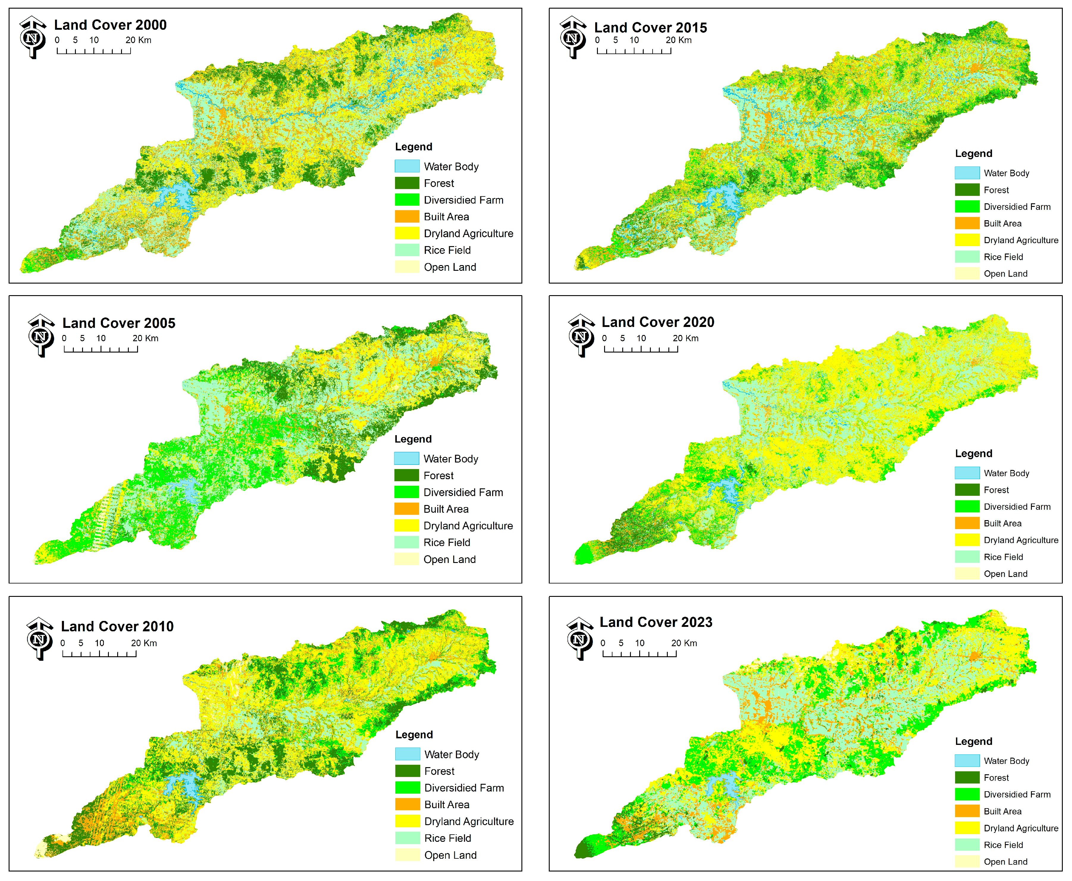
Table 3 presents temporal changes in land cover within the Klambu catchment area from 2000 to 2023. Notably, water bodies exhibited fluctuations, decreasing from 51.8 km2 in 2000 to 24.2 km2 in 2005, before gradually increasing to 39.5 km2 by 2023. Forest areas experienced a sharp decline from 523.2 km2 in 2000 to just 107.5 km2 in 2020, followed by a modest recovery to 137.2 km2 by 2023. Rice fields remained a significant land cover type but showed a slight decrease from 1091.7 km2 in 2000 to 1014.1 km2 in 2023. Conversely, dry agriculture expanded, reaching a peak of 1217.3 km2 in 2020, reflecting a shift in land use practices over time. These fluctuations are unlikely to reflect actual land-use dynamics alone; rather, they point to methodological inconsistencies. A primary factor is the image classification approach, which is highly sensitive to the quality and spectral characteristics of the input imagery. Early years (2000 and 2005) relied on Landsat 6 and Landsat 7, which have lower radiometric resolution and more frequent data gaps (e.g., SLC-off issue in Landsat 7). From 2010 onward, the transition to Landsat 8 introduced improved sensor capabilities, including higher radiometric fidelity and better atmospheric correction, resulting in more accurate delineation of complex classes such as built-up areas and forest canopy. Variations in preprocessing, seasonal acquisition, and classifier training further amplify these discrepancies. In short, the anomalies in Built Area and Forest are driven by sensor evolution and classification sensitivity, rather than abrupt real-world land cover changes. Future studies should apply consistent classification algorithms, robust training datasets, and cross-sensor harmonization techniques to minimize such artifacts and ensure temporal comparability.
These trends are critical for understanding the relationship between land cover dynamics and hydrological processes in the region. The spatial representation of the data is shown in Figure 2.
The Cellular Automata–Markov Chain (CA–Markov) approach was employed to simulate spatial and temporal dynamics of land cover change. Historical raster maps for 2000 and 2010 were first subjected to geometric correction and reclassification into six categories: urban/built area, agriculture, forest, water bodies, grassland and bare soil using ArcGIS 10.8 [36]. These standardized 30 × 30 m layers served as inputs to the Land Change Modeller within IDRISI Selva. Transition probability matrices were derived from observed changes between 2000 and 2010 via Markov chain analysis [29]. A 3 × 3 Moore neighborhood was applied to capture local cell interactions, so that the state of each pixel was influenced by its eight adjacent neighbors [48].
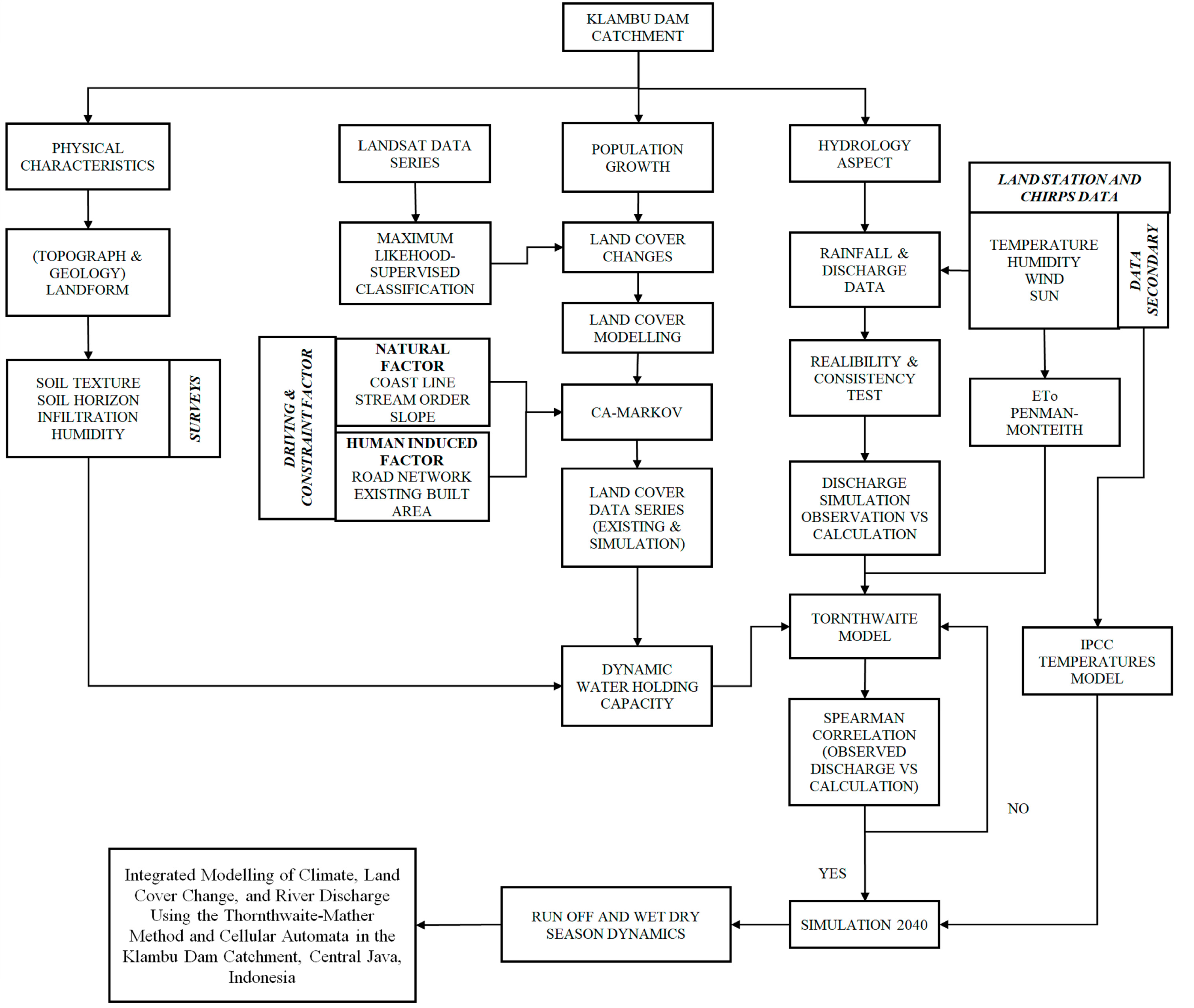
A conceptual framework showing components and relationships was used as a framework for analyzing hydrology in the study (Figure 3).
Driving factors such as distance to roads, proximity to urban centers and slope gradient were incorporated through logistic regression, with coefficients calibrated by maximizing the area under the receiver operating characteristic curve (AUC) [48]. Population count was integrated into the built-up area analysis using the Kernel Density tool in GIS, enabling spatial representation of demographic concentration as a continuous surface. This approach supports modeling urban growth patterns by linking population intensity to land development dynamics. Constraints, including protected zones (e.g., riparian buffers along the Kaligarang River) and slopes exceeding 30°, were implemented as binary masks to prevent implausible transitions, such as urban growth in steep terrain or within conservation areas [45]. In this research using key assumptions, driving factors remain stationary over time (e.g., road networks and urban boundaries follow projected trends without abrupt change).
Model calibration involved comparing the simulated 2010 output against the actual 2010 land cover map, yielding a Cohen’s Kappa coefficient of 0.82, indicative of strong agreement [38]. Discrepancies, particularly an overestimation of agricultural loss on steep slopes, were addressed by adjusting neighborhood weightings and refining slope thresholds [55]. Validation was further conducted by generating a simulated 2020 map and comparing it to observed 2020 data using ROC analysis, which produced an AUC of 0.78 for urban expansion [48]. Monte Carlo simulations within the LCM quantified uncertainty, indicating a ±5% margin of error in transition probabilities [38].

2.3.3. Impacts of Climate and Land Use Projections on Discharge

To assess future river discharge under combined land cover and climate-change influences, the projected 2020–2040 land cover maps from the CA–Markov model were overlaid with climate projections from selected IPCC scenarios (e.g., RCP 1–8). Monthly precipitation (P) and temperature (T) for 2020–2040 were extrapolated from historical observations (1990–2020) through simple linear regression:
P f u t u r e = m p × y e a r + c p , T f u t u r e = m t × y e a r + c t
Coefficients mp, mt (slopes) and cp, ct (intercepts) calibrated to IPCC RCP 1–8 trends.
Projections bias-corrected against regional climate model outputs.
The workflow comprised:
  • Land Cover Forcing: Raster layers of future land cover classes were translated into hydrological parameters—imperviousness, infiltration rates and roughness coefficients according to established lookup tables [55].
  • Climate Forcing: Monthly climate projections were processed to generate design storm events and long-term precipitation series consistent with each IPCC scenario [43].
  • Hydrological Simulation: The hydrological model used both sets of inputs to simulate runoff generation, channel routing and baseflow dynamics [40].
  • Scenario Analysis: River discharge outputs were evaluated across multiple climate scenarios to quantify the relative influence of land cover change, climate variability, and their combined effects on hydrological conditions. To assess future climate impacts under varying emission trajectories, this study employs a set of standardized scenarios from the IPCC AR6 framework, representing a continuum from low to very high radiative forcing pathways. These include Scenario 2.6 (C3), Scenario 4.5 (C6), Scenario 7.0 (C7), and Scenario 8.5 (C8), which collectively capture a broad range of projected changes in temperature and precipitation. Although these scenarios are coded using the SSP–RCP naming convention, the present study focuses primarily on their climatic forcing outputs, rather than their socioeconomic narratives. This approach provides a robust basis for evaluating future shifts in wet and dry season intensity and their potential impacts on erosion, runoff generation, and the long-term service life of the Klambu Dam catchment.
The selection of the Cellular Automata–Markov Chain (CA–Markov) model and the Thornthwaite–Mather water balance approach was guided by data availability, spatial scale, and the objectives of this study. The CA–Markov model was chosen for land cover projection because it effectively captures temporal transition probabilities while preserving spatial neighborhood relationships, which are critical in agricultural and peri-urban catchments. Unlike data-intensive approaches such as artificial neural networks or agent-based models, CA–Markov relies on historical land cover data, making it suitable for regions where long-term socioeconomic and policy datasets are limited.
Similarly, the Thornthwaite–Mather method was selected to assess hydrological responses due to its robustness for long-term water balance estimation in data-scarce environments. While physically based hydrological models such as SWAT or VIC provide detailed process representation, they require extensive input data that are often unavailable or inconsistent in tropical catchments. The Thornthwaite–Mather approach, which primarily depends on temperature and precipitation, aligns well with the available ground and satellite-based climate data and is appropriate for evaluating seasonal and interannual variations in water availability. Given the study’s focus on long-term hydrological trends and management implications rather than event-scale simulations, this approach provides a reliable and practical framework.

3. Result and Discussion

3.1. Air Temperature and Precipitation Trends

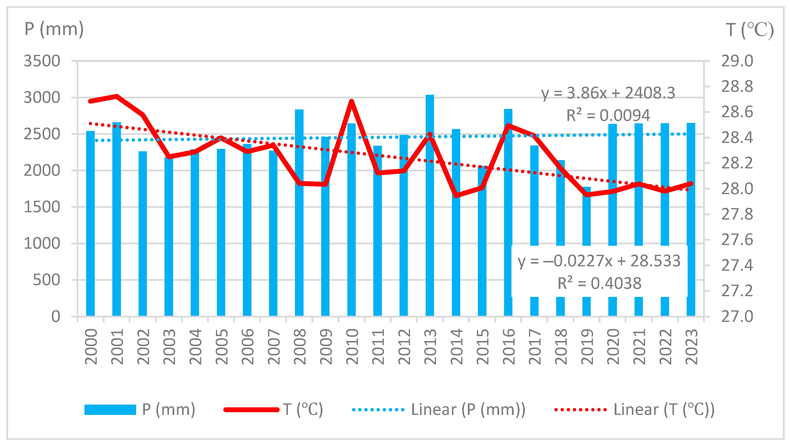
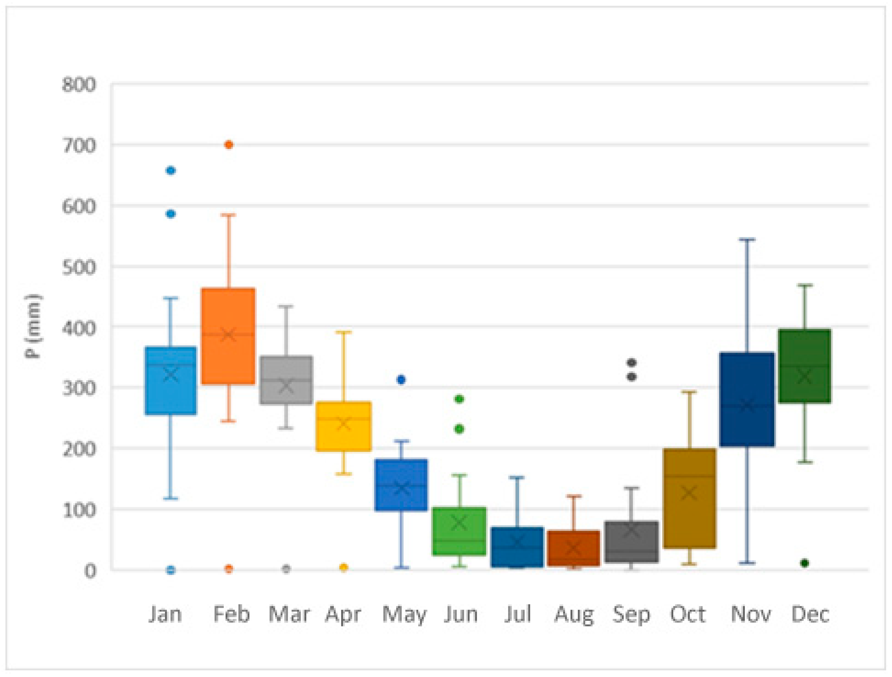
The Klambu Dam Catchment Area in Central Java, Indonesia, has undergone notable climatic fluctuations over the past two decades. Between 2005 and 2023, temperature trends exhibited substantial interannual variability rather than a linear progression. Although the average annual temperature decreased slightly from 28.25 °C in 2005 to 28.04 °C in 2023, extreme values were recorded—reaching 28.68 °C in 2012 and dipping to 27.95 °C in 2021. Concurrently, rainfall variability increased by approximately 17%, characterized by more intense wet-season precipitation and prolonged dry spells. These patterns, illustrated in Figure 4, Figure 5 and Figure 6, underscore the shifting hydroclimatic regime of the study area.
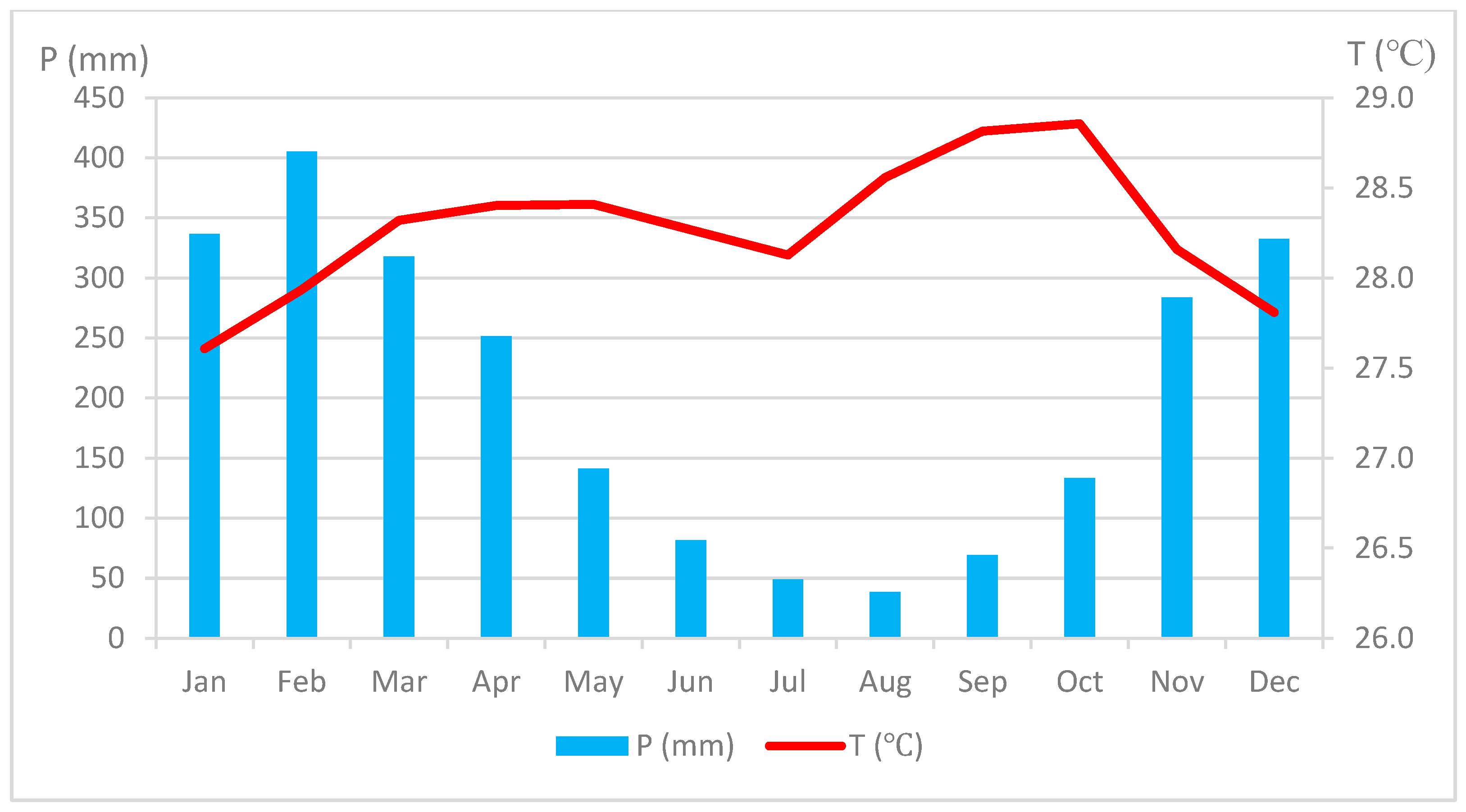
In 2015, nearly the lowest annual rainfall totals and nearly the lowest average air temperature were recorded, while in 2010, rainfall was higher than the multi-year average, while air temperature was among the highest. On an annual basis, the highest average annual air temperature was recorded in the summer months of August, September, and October, while the lowest was recorded in December, January, and February. Average monthly precipitation shows greater variation throughout the year. The wet season occurs from November to April, with monthly rainfall totals ranging from 133 mm to 405 mm. During the dry season, average monthly rainfall totals are significantly lower, ranging from 38 mm to 81 mm.
Precipitation totals in individual months of the year show significant variation, as seen in Figure 4. The outliers in precipitation totals are particularly noticeable in September, where in two years (2010 and 2016) precipitation totals for a given month were more than three times higher than the average for the 2000–2023 multi-year period. Similar situations occurred in January, February, May, and June (Figure 6).
Climate data from 2000 to 2023 was utilized to construct a predictive model of temperature trends, which was then extended to 2040. The modeling was conducted using linear regression methods aligned with scenarios from the [43] IPCC. The simulation results indicate an increasing temperature trend of approximately 0.1% per year over the observed period. This temperature increase is consistent with the findings of the Intergovernmental Panel on Climate Change in its Sixth Assessment Report (AR6), which projects that tropical regions such as Indonesia will experience an increase in surface temperature as a result of growing greenhouse gas concentrations [43]. This temperature increase has the potential to significantly impact hydrological dynamics in the Klambu Dam area.

3.2. Changes in Land Cover and Use

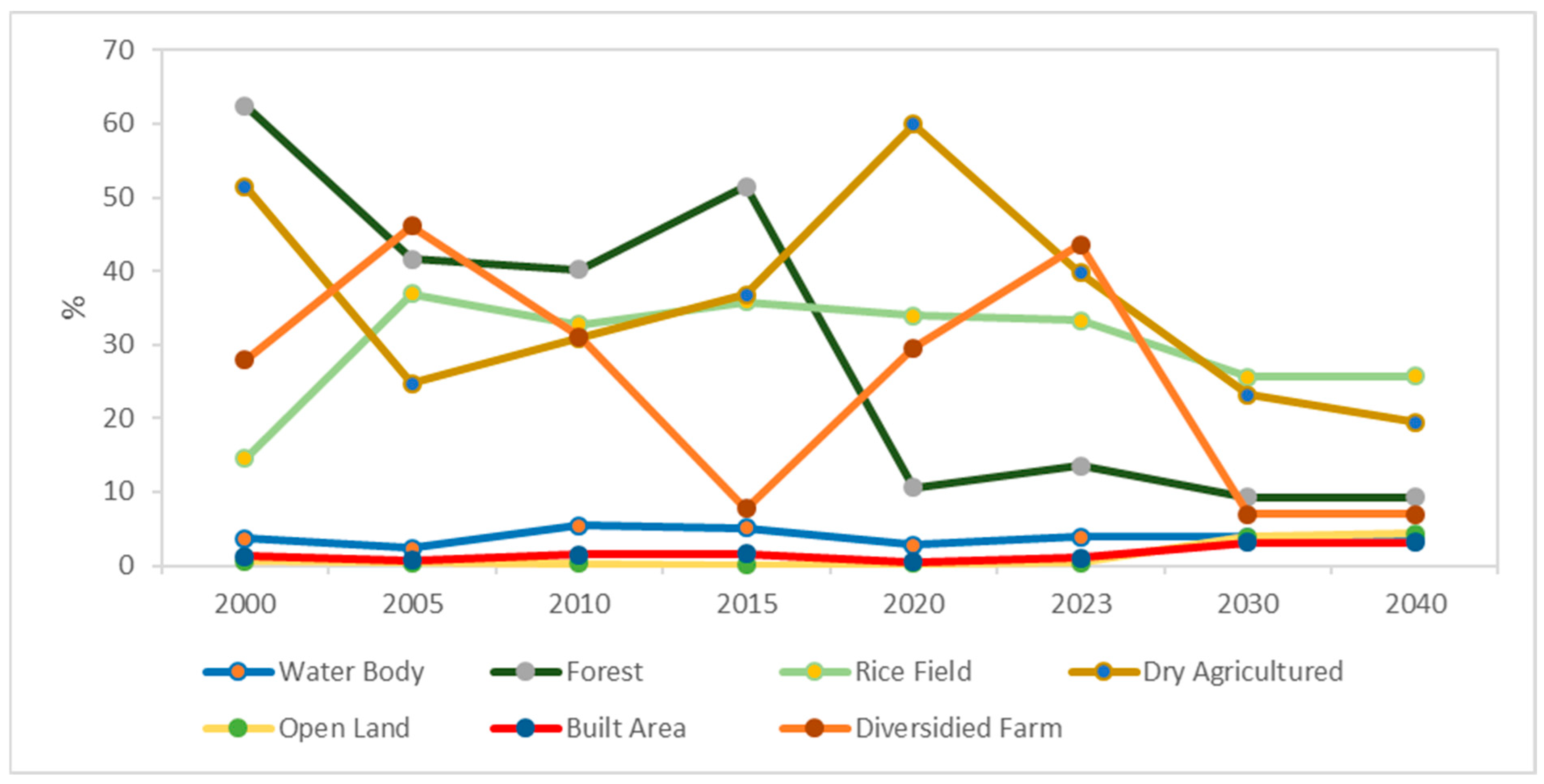
From 2000 to 2023 significant changes in land cover were observed in the Klambu Dam Catchment Area. Forests experienced the most significant decrease in area, from 523.2 km2 (2000) to 137.2 km2 (2023). Conversely, mixed farming exhibited a substantial increase, rising from 117.0 km2 to 664.4 km2 during the same period. The area dedicated to paddy fields has been observed to undergo fluctuations, with a decrease from 1091.7 km2 in the year 2000 to 1014.1 km2 in 2023. In the year 2023, the area dedicated to dryland agriculture (807.4 km2) surpassed the level observed in 2000 (748.2 km2). Concurrently, the extent of open land experienced an increase from 16.7 km2 to 64.3 km2. Conversely, settlements exhibited a declining trend, with a decrease from 497.0 km2 in 2000 to 319.0 km2 in 2023 (Figure 7). Subsequently, the historical data was modelled up to 2030 and 2040 using the Cellular Automata-Markov Chain method, resulting in a wide array of trends. This can be seen in Figure 8. Projections indicate an anticipated escalation in dryland agriculture, with an estimated increase from 396.0 km2 (2030) to 470.7 km2 (2040). Conversely, the area of open land is predicted to diminish from 666.6 km2 to 596.4 km2. Conversely, other land cover types, including water bodies, forests, rice fields, settlements, and mixed gardens, are projected to exhibit minimal fluctuations over the ten-year span.

3.3. Water Resources

The following research was conducted to ascertain the impact of climate change on water resources in the Klambu Dam area. The study employed two distinct data sets: historical (2000–2023) and simulation (2024–2040). These data sets were then analyzed to understand the dynamics of climate change and land cover. The Thornthwaite-Matters method was then employed to calculate the annual mainstay discharge. This calculation was then compared with the observed discharge at Klambu Dam. In this calculation, four primary years are utilized to model the mainstay discharge. This is achieved by adjusting the field observation discharge data presented in Table 2.
Subsequently, with reference to the four primary years contained in Table 2, the discharge is calculated using the Thornthwaite-Matters method. This calculation involves the evaluation of each component that affects the catchment area system, including rainfall, temperature, actual evaporation, and river flow. The calculated components are integrated to form a water balance system that produces runoff data. Subsequently, the runoff data undergoes adjustment to align with the conditions of the catchment area, employing an assumption of 50% in each month. In instances where residual runoff is observed, it is typically discharged in the subsequent month. Therefore, a series of calculations is performed to obtain a monthly discharge. This discharge is then compared with the observed discharge using the Pearson comparison method. The results of this study are presented in Table 4.
The correlation values ranged from 0.57 to 0.94, suggesting a high degree of variability in model performance across years. This variability may reflect temporal inconsistencies in climatic inputs or land surface processes not fully captured by the Thornthwaite-Mather method. The variation in these results indicates that each year exhibits a significant difference in each Thorntwaite-Matters model. Consequently, the most optimal model selection is achieved by considering the Pearson value between the observed discharge and the Thorntwaite-Matters model discharge, specifically in the year 2015. The model selection is intended to be applied to all years utilized in this study (2000–2040). The objective is to generate the discharge data that is enumerated in Table 5.

3.4. Discussion

The temporal distribution of rainfall in the Klambu Dam Catchment reveals a consistent seasonal pattern distinguishing wet and dry months, with notable variability across the examined years (2000–2040) (Table 6). The wet season predominantly occurs from January to April and resumes in November–December, marked by high rainfall intensities exceeding 150 mm/month. Conversely, the dry season spans from May to October, characterized by a sharp decline in precipitation, with several months registering less than 30 mm/month, particularly July to September. Notably, rainfall in September has shown anomalous peaks, such as 70.92 mm in 2010, suggesting occasional mid-dry-season anomalies possibly driven by climatic disturbances. The temporal shift in rainfall onset and retreat is apparent in 2040, where April rainfall significantly declined to 161.52 mm compared to over 220 mm in earlier years, indicating a shortened wet season. This shift may result in delayed planting cycles and increased drought exposure.
The Pearson correlation coefficients (Table 4), comparing simulated and observed discharge, range from 0.572 to 0.943, suggesting generally strong model performance, though with variability. The lowest correlation (0.572) in 2020 may be attributed to mid-season rainfall anomalies and higher interannual climate variability. In contrast, the model performed best in 2015, with correlations of 0.943, indicating reliable water balance simulation during those years. Overall, the results suggest that although total rainfall volumes remain relatively stable, intra-annual distribution shifts could significantly affect water availability, hydropower regulation, and agricultural planning in the region. This underlines the importance of adaptive management strategies and continuous monitoring under changing climatic conditions.
The findings of this study, derived from an integrated analysis of discharge simulations, utilized the Thornthwaite-Mather method, IPCC climate projections, and Cellular Automata–Markov Chain modeling of land cover dynamics. The results provided a set of interrelated insights that offer a nuanced understanding of hydrological responses within the study area. The simulation outputs indicated that variations in land cover and soil type had limited influence on discharge estimations within the Thornthwaite-Mather framework. In contrast, climatological variables, particularly precipitation and temperature exerted a substantial determinative effect. The method’s limitations became evident through statistical evaluation, where Pearson correlation coefficients demonstrated considerable year-to-year variability, indicating unreliable monthly discharge projections compared to observed data at Klambu Dam.
Projected seasonal distribution shifts in the Klambu Dam catchment under IPCC AR6 radiative forcing scenarios reveal substantial temporal alterations in rainfall patterns. Under the low-forcing scenario (C3/2.6 W·m−2), the wet months remain concentrated between January–April and November–December, closely resembling historical hydrological conditions (Table 7). In contrast, the moderate-forcing scenarios (C5 and C6/~4.5 W·m−2) show a contraction of the wet season, with transitional months such as April and November shifting to dry conditions by 2040, thereby extending the dry season from May to November. Under the high-forcing scenario (C7–C8/≥7.0–8.5 W·m−2), the wet season is projected to shrink drastically to only January–March, with April and even December becoming dry by 2045, resulting in a prolonged nine-month dry season. Such shifts imply heightened drought probability, reduced baseflow and runoff, and increased pressure on agricultural production and reservoir storage capacity. These findings demonstrate the necessity of integrating AR6 climate-forcing projections into watershed planning, and they highlight the urgency of implementing adaptive water-resource strategies to maintain hydrological resilience in the Klambu Dam system.
Although the Thornthwaite-Mather model showed limitations in capturing precise monthly discharge dynamics—evidenced by variability in Pearson correlation coefficients—it remains a practical tool for assessing overall water balance and runoff trends. Its simplicity and reliance on widely available climate data make it suitable for data-scarce regions. The Thornthwaite and Mather water balance method is widely used worldwide, including in Indonesia [56,57,58]. However, as some authors point out, the results of studies using the Thornthwaite and Mather water balance method require verification. Verification should apply not only to the input data but also to a range of climate data covering at least 25–30 years [59,60]. The model outputs, such as an estimated discharge of 66.99 m3/s, support crucial water uses in the Klambu Dam Catchment, including agricultural irrigation, domestic supply through the Klambu–Kudu transmission system, and small-scale hydropower. Notably, while volumetric discharge is projected to remain relatively stable, temporal shifts in wet and dry months could impact agricultural and aquaculture activities. These findings underscore the importance of adaptive water management to mitigate the risks of seasonal water scarcity and crop failure. Studies conducted in Iran for various catchments have shown that land use changes within individual catchments may have varying degrees of impact on future extreme flows [61]. Therefore, it is crucial to monitor land use changes locally, which will ultimately help mitigate the risk of seasonal water shortages and crop failures.

3.5. Implications for Water Resource Management and Adaptive Strategies

The projected seasonal shifts in rainfall and discharge have important implications for water resource management in the Klambu Dam Catchment. Although total annual water availability is expected to remain relatively stable, the shortening of the wet season and extended dry periods increase vulnerability to dry-season water shortages, particularly for irrigation, aquaculture, and domestic supply. These findings highlight the need to transition from volume-based planning toward seasonally adaptive water management approaches that explicitly account for climate non-stationarity. For reservoir operation, adaptive rule curves that consider shifting inflow timing should be implemented to improve system reliability. Storing a larger proportion of wet-season inflows and applying more conservative release strategies during transitional months, especially at the onset of the dry season, can help mitigate dry-season shortages. Incorporating climate-based seasonal forecasts into reservoir operation planning would further enhance resilience under increasing hydroclimatic variability [57].
In the agricultural sector, adjustments to cropping calendars and crop selection are necessary to align with evolving rainfall patterns. Promoting less water-intensive crops during prolonged dry periods and improving irrigation efficiency through optimized scheduling and modern irrigation practices can substantially reduce water stress. In addition, land cover management plays a critical role in long-term watershed resilience. Forest conservation, reforestation, and agroforestry practices in upstream areas can enhance infiltration, reduce surface runoff, and help sustain baseflow during dry seasons.
Overall, integrating climate projections, land cover dynamics, and hydrological responses provides a practical framework for adaptive watershed management. Strengthened coordination among water authorities, agricultural agencies, and land use planners is essential to translate these findings into effective management strategies and enhance the resilience of the Klambu Dam Catchment to future hydroclimatic uncertainty.
Despite its effectiveness in capturing long-term water balance dynamics, the Thornthwaite–Mather model has inherent limitations, particularly in representing short-term hydrological variability. The model relies on monthly temperature and precipitation inputs and simplified soil moisture accounting, which restricts its ability to resolve intra-monthly processes such as extreme rainfall events, rapid runoff generation, and short-duration droughts. Consequently, discrepancies may arise when comparing simulated monthly discharge with observed values, especially during transitional wet–dry periods. To improve temporal resolution and predictive accuracy, future studies could integrate the Thornthwaite–Mather framework with complementary approaches, such as physically based hydrological models (e.g., SWAT or HEC-HMS), daily water balance models, or satellite-based evapotranspiration products (e.g., MODIS ET). Additionally, coupling the model with stochastic rainfall disaggregation or climate downscaling techniques may enhance its applicability for sub-monthly analysis. Such integrated modeling strategies would allow more robust representation of hydrological extremes while retaining the practical advantages of the Thornthwaite–Mather approach in data-scarce tropical watersheds.

4. Conclusions

This study presents an integrated assessment of hydrological responses in the Klambu Dam Catchment under combined climate variability and land cover change from 2000 to 2040, using the Thornthwaite–Mather water balance method, IPCC-based climate projections, and land use simulations derived from a Cellular Automata–Markov Chain model. The results indicate that although total annual discharge is projected to remain relatively stable, pronounced temporal shifts in seasonal flow patterns are expected. A contraction of the wet season and extended dry periods—particularly during transitional months such as April—highlight increasing climate-driven pressure on dry-season water availability.
Land cover changes, especially forest reduction and agricultural expansion, further influence runoff and infiltration processes, amplifying changes in streamflow timing rather than total volume. Model validation demonstrates variable performance across years, emphasizing the need for localized calibration, although the Thornthwaite–Mather method remains suitable for long-term planning in data-scarce tropical watersheds. Overall, the findings underscore the importance of integrated climate–land use–hydrological approaches to support adaptive watershed and reservoir management, strengthen land cover conservation, and enhance resilience to future hydroclimatic uncertainty.

Author Contributions

Conceptualization, F.H.; methodology, F.H., M.F.R. and D.P.; software, L.A.W., M.F.R. and D.P.; validation, F.H., M.F.R. and D.P.; formal analysis, F.H., M.F.R., D.P. and K.K.-W.; investigation, F.H., M.F.R. and D.P.; resources, F.H., M.F.R. and D.P.; data curation, F.H., M.F.R. and D.P.; writing—original draft preparation, F.H. and K.K.-W.; writing—review and editing, F.H. and K.K.-W.; visualization, F.H., L.A.W., M.F.R., D.P. and K.K.-W.; supervision, F.H., L.A.W., M.F.R., D.P. and K.K.-W.; project administration, K.K.-W.; funding acquisition, K.K.-W. All authors have read and agreed to the published version of the manuscript.

Funding

This research was financially supported by DIPA (Daftar Isian Pelaksanaan Anggaran/Budget Implementation List) of Universitas Negeri Semarang, Decree Letter Number T/237/UN37/HK.02/2024 dated 20 February 2024, and Basic Research Contract Number 54.26.2/UN37/PPK.10/2024 dated 26 February 2024.

Data Availability Statement

The hydrological data for the Klambu Dam catchment were obtained from the Balai Besar Wilayah Sungai (BBWS) Bengawan Solo (https://bbwsbengawansolo.id/ (accessed on 1 February 2024) and BBWS Pemali Juana (https://bbwspena.site/balai/bbwspemalijuana/pages/profil_bbwspj (accessed on 1 February 2024), Ministry of Public Works and Housing, Indonesia. These data are not publicly available and can only be accessed on-site at the BBWS’ office upon formal request and approval from the authority in charge. Some of the climatic data (precipitation and temperature) were obtained from the Climate Hazards Group Infra Red Precipitation with Station data (CHIRPS), which is freely available at https://www.chc.ucsb.edu/data/chirps (accessed on 7 August 2023). Processed datasets generated during the current study (e.g., land cover classifications from Landsat imagery and hydrological simulation outputs) are available from the corresponding author upon reasonable request.

Acknowledgments

The authors would like to express their sincere gratitude to the Lembaga Penelitiandan Pengabdiankepada Masyarakat (LPPM), Universitas Negeri Semarang (UNNES) for providing research funding. Special thanks are also extended to Geopioneer for their valuable assistance in the field surveying. The authors are deeply grateful to all colleagues and individuals who contributed their support and insights throughout this research but cannot be mentioned individually one by one.

Conflicts of Interest

The authors declare no conflicts of interest.

References

  1. Kubiak-Wójcicka, K. Variability of Air Temperature, Precipitation and Outflows in the Vistula Basin (Poland). Resources 2020, 9, 103. [Google Scholar] [CrossRef]
  2. Di Nunno, F.; Diodato, N.; Bellocchi, G.; Tricarico, C.; de Marinis, G.; Granata, F. Evapotranspiration Analysis in Central Italy: A Combined Trend and Clustering Approach. Climate 2024, 12, 64. [Google Scholar] [CrossRef]
  3. Abbas, Z.; Yang, G.; Zhong, Y.; Zhao, Y. Spatiotemporal Change Analysis and Future Scenario of LULC Using the CA-ANN Approach: A Case Study of the Greater Bay Area, China. Land 2021, 10, 584. [Google Scholar] [CrossRef]
  4. Saddique, N.; Mahmood, T.; Bernhofer, C. Quantifying the impacts of land use/land cover change on the water balance in the afforested River Basin, Pakistan. Environ. Earth Sci. 2020, 79, 448. [Google Scholar] [CrossRef]
  5. Engida, T.G.; Nigussie, T.A.; Aneseyee, A.B. Land Use/Land Cover Change Impact on Hydrological Process in the Upper Baro Basin, Ethiopia. Hindawi Appl. Environ. Soil Sci. 2021, 2021, 6617541. [Google Scholar] [CrossRef]
  6. Obahoundje, S.; Diedhiou, A. Potential impacts of climate, land use and land cover changes on hydropower generation in West Africa: A review. Environ. Res. Lett. 2022, 17, 043005. [Google Scholar] [CrossRef]
  7. Garg, V.; Prasun, S.P.A.; Bhaskar, K.G. Assessment of land use land cover change impact on hydrological regime of a basin. Environ. Earth Sci. 2017, 76, 635. [Google Scholar] [CrossRef]
  8. Hu, J.; Wu, Y.; Wang, L.; Sun, P.; Zhao, F.; Jin, Z.; Wang, Y.; Qiu, L.; Lian, Y. Impacts of land-use conversions on the water cycle in a typical watershed in the southern Chinese Loess Plateau. J. Hydrol. 2021, 593, 125741. [Google Scholar] [CrossRef]
  9. Kimbi, S.B.; Onodera, S.-I.; Wang, K.; Kaihotsu, I.; Shimizu, Y. Assessing the Impact of Urbanization and Climate Change on Hydrological Processes in a Suburban Catchment. Environments 2024, 11, 225. [Google Scholar] [CrossRef]
  10. Costa, M.H.; Botta, A.; Cardille, J.A. Effects of large-scale changes in land cover on the discharge of the Tocantins River, Southeastern Amazonia. J. Hydrol. 2003, 283, 206–217. [Google Scholar] [CrossRef]
  11. Li, D.; Long, D.; Zhao, Y.; Lu, H.; Hong, Y. Observed changes in flow regimes in the Mekong River basin. J. Hydrol. 2017, 551, 217–232. [Google Scholar] [CrossRef]
  12. Zhang, X.; Zhang, L.; Zhao, J.; Rustomji, P.; Hairsine, P. Responses of streamflow to changes in climate and land use/cover in the Loess Plateau, China. Water Resour. Res. 2014, 50, 3205–3220. [Google Scholar] [CrossRef]
  13. Arnell, N.W.; Gosling, S.N. The impacts of climate change on river flow regimes at the global scale. J. Hydrol. 2016, 534, 387–394. [Google Scholar] [CrossRef]
  14. Bronstert, A.; Niehoff, D.; Bürger, G. Effects of climate and land-use change on storm runoff generation: Present knowledge and modelling capabilities. Hydrol. Process. 2002, 16, 509–529. [Google Scholar] [CrossRef]
  15. Vaze, J.; Teng, J.; Chiew, F.H.S. Impact of climate change on runoff in the Murray-Darling Basin: A simulation study. Water Resour. Res. 2011, 47, W00G10. [Google Scholar] [CrossRef]
  16. Feyen, L.; Dankers, R. Impact of global warming on streamflow drought in Europe. J. Geophys. Res. Atmos. 2009, 114, D17116. [Google Scholar] [CrossRef]
  17. Scanlon, B.R.; Keese, K.E.; Flint, A.L.; Flint, L.E.; Gaye, C.B.; Edmunds, W.M.; Simmers, I. Global synthesis of groundwater recharge in semiarid and arid regions. Hydrol. Process. 2006, 20, 3335–3370. [Google Scholar] [CrossRef]
  18. Wang, G.Q.; Zhang, J.Y.; Jin, J.L.; Pagano, T.C.; Calow, R.; Bao, Z.X.; Liu, C.S.; Liu, Y.L.; Yan, X.L. Assessing water resources in China using PRECIS projections and a VIC model. Hydrol. Earth Syst. Sci. 2012, 22, 231–250. [Google Scholar] [CrossRef]
  19. Kubiak-Wójcicka, K.; Piątkowski, K.; Juśkiewicz, W.W. Lake surface changes of the Osa River catchment, (northern Poland), 1900–2010. J. Maps 2021, 17, 18–29. [Google Scholar] [CrossRef]
  20. Wang, J.; Bretz, M.; Dewan, M.M.A.; Delavar, M.A. Machine learning in modelling land-use and land cover-change (LULCC): Current status, challenges and prospects. Sci. Total Environ. 2022, 822, 153559. [Google Scholar] [CrossRef]
  21. Shukla, S.; Meshesha, T.W.; Sen, I.S.; Bol, R.; Bogena, H.; Wang, J. Assessing Impacts of Land Use and Land Cover (LULC) Change on Stream Flow and Runoff in Rur Basin, Germany. Sustainability 2023, 15, 9811. [Google Scholar] [CrossRef]
  22. Barati, A.A.; Zhoolideh, M.; Azadi, H.; Ju-Hyoung Lee, J.-H.; Scheffran, J. Interactions of land-use cover and climate change at global level: How to mitigate the environmental risks and warming effects. Ecol. Indic. 2023, 146, 109829. [Google Scholar] [CrossRef]
  23. Cook, J.; Oreskes, N.; Doran, P.T.; Anderegg, W.R.L.; Verheggen, B.; Maibach, E.W.; Carlton, J.S.; Lewandowsky, S.; Skuce, A.G.; Green, S.; et al. Consensus on consensus: A synthesis of consensus estimates on human-caused global warming. Environ. Res. Lett. 2016, 11, 048002. [Google Scholar] [CrossRef]
  24. Verma, S.; Verma, M.K.; Prasad, A.D.; Mehta, D.; Azamathulla, H.M.; Muttil, N.; Rathnaynake, U. Simulating the Hydrological Processes under Multiple Land Use/Land Cover and Climate Change Scenarios in the Mahanadi Reservoir Complex, Chhattisgarh, India. Water 2023, 15, 3068. [Google Scholar] [CrossRef]
  25. Wardhani, F.A.; Pravitasari, A.E.; Ridwansyah, I. Flash flood assessment at Upper Cisadane Watershed using land use/land cover and morphometric factors. In IOP Conference Series: Earth and Environmental Science; IOP Publishing: Bristol, UK, 2022; Volume 1109, p. 012002. [Google Scholar] [CrossRef]
  26. Kurniawan, T.A.; Bandala, E.R.; Othman, M.H.D.; Goh, H.H.; Anouzlae, A.; Chewf, K.W.; Aziz, F.; Al-Hazm, H.E.; Nisa’ulKhoir, A. Implications of climate change on water quality and sanitation in climate hotspot locations: A case study in Indonesia. Water Supply 2024, 24, 517. [Google Scholar] [CrossRef]
  27. Umami, A.; Sukmana, H.; Wikurendra, E.A.; Paulik, E. A review on water management issues: Potential and challenges in Indonesia. Sustain. Water Resour. Manag. 2022, 8, 63. [Google Scholar] [CrossRef]
  28. Anggraheni, E.; Hamdany, A.H.; Maricar, F.; Andika, N.; Sisinggih, D.; Tanlie, F.S.; Respati, F.A.R. Hydrological Response of Land Use and Climate Change Impact on Sediment Rate in Upper Citarum Watershed. Fluids 2025, 10, 36. [Google Scholar] [CrossRef]
  29. Gradiyanto, F.; Parmantoro, P.N.; Suharyanto. Impact of climate change on Kupang River flow and hydrological extremes in Greater Pekalongan, Indonesia. Water Sci. Eng. 2025, 18, 69–77. [Google Scholar] [CrossRef]
  30. Pranata, K.A.; Aji, A. Analisis Spasial Tingkat Potensi Kekeringan dan Tingkat Kesiapsiagaan Masyarakat dalam Menghadapi Bencana Kekeringan di Kabupaten Grobogan. Indones. J. Conserv. 2021, 10, 108–114. [Google Scholar]
  31. Ikhwali, M.F.; Pawattana, C.; Nur, S.; Azhari, B.; Ikhsan, M.; Aida, N.; Silvia, C.S. Reviews, challenges, and prospects of the application of Hydrologic Engineering Center-Hydrologic Modelling System (HEC-HMS) model in Indonesia. Eng. Appl. Sci. Res. 2022, 49, 669–680. [Google Scholar] [CrossRef]
  32. Avia, L.Q. Change in rainfall per-decades over Java Island, Indonesia. In IOP Conference Series: Earth and Environmental Science; IOP Publishing: Bristol, UK, 2019. [Google Scholar] [CrossRef]
  33. Yanto; Livneh, B.; Rajagopalan, B.; Kasprzyk, J. Hydrological model application under data scarcity for multiple watersheds, Java Island, Indonesia. J. Hydrol. Reg. Stud. 2017, 9, 127–139. [Google Scholar] [CrossRef]
  34. Pratiwi, E.P.A.; Ramadhani, E.L.; Nurrochmad, F.; Legono, D. The Impacts of Flood and Drought on Food Security in Central Java. J. Civ. Eng. Forum 2020, 6, 69–78. [Google Scholar] [CrossRef]
  35. Prihestiwi, R.C.; Handayani, W.; Sarasadi, A. Land Use and Surface Runoff Change in Babon Watershed Semarang Greater Area. In IOP Conference Series: Earth and Environmental Science; IOP Publishing: Bristol, UK, 2023. [Google Scholar] [CrossRef]
  36. Ozturk, D. Urban growth simulation of Atakum (Samsun, Turkey) using cellular automata-Markov chain and Multi-layer Perceptron-Markov chain models. Remote Sens. 2015, 7, 5918–5950. [Google Scholar] [CrossRef]
  37. Mukesh, K.; Shiva Nagendra, S.M. Artificial Neural Networks in Vehicular Pollution Modelling; Springer: Berlin/Heidelberg, Germany, 2007; 242p. [Google Scholar]
  38. Eastman, J.R. IDRISI Selva Tutorial. Worcester: IDRISI Production, Clark Labs-Clark University. 2015. Available online: http://uhulag.mendelu.cz/files/pagesdata/eng/gis/idrisi_selva_tutorial.pdf (accessed on 20 September 2025).
  39. Hanafi, F. Kajian perubahan penggunaan lahan terhadap laju erosi permuka an di daerah tangkapan air waduk mrica. J. Geogr. Media Inf. Pengemb. Ilmudan Profesi Kegeografian 2015, 12, 1–14. [Google Scholar]
  40. BBWS Pemali Juana. Profil BBWS Pemali Juana. 2022. Available online: https://sda.pu.go.id/balai/bbwspemalijuana/pages/profil_bbwspj (accessed on 10 September 2025).
  41. Rahadeyani, R.D.; Johanes Kodoatie, R.J.; Atmodjo, P.S. Strategi Penanganan Aspek Non Teknis Dalam Infrastruktur Saluran Air Baku Klambu-Kudu. Briliant J. Ris. Konseptual 2020, 5, 591–601. [Google Scholar] [CrossRef]
  42. Sarwanta, S.; Abdulgani, H. Penyusunan Penilaian Kinerja Dan Angka Kebutuhan Nyata Operasi Dan Pemeliharaan (AKNOP) Daerah Irigasi Klambu. J. Rekayasa Infrastruktur 2021, 7, 25–29. [Google Scholar] [CrossRef]
  43. Intergovernmental Panel on Climate Change (IPCC). Synthesis Report, Summary for Policymakers. Contribution of Working Groups I, II and III to the Sixth Assessment Report of the Intergovernmental Panel on Climate Change; Core Writing Team, Lee, H., Romero, J., Eds.; IPCC: Geneva, Switzerland, 2023; Available online: https://www.ipcc.ch/report/ar6/syr/downloads/report/IPCC_AR6_SYR_SPM.pdf (accessed on 20 September 2025).
  44. Julianto, F.D.; Ediyanto, I. Analisis Sebaran Potensi Kekeringan Dengan Cloud Computing Platform di Kabupaten Grobogan. J. Ilm. Tek. Geomatika IMAGI 2021, 1, 23–30. [Google Scholar] [CrossRef]
  45. Hanafi, F.; Rahmadewi, D.P.; Setiawan, F. Land Cover Changes Based on Cellular Automata for Land Surface Temperature in Semarang Regency. Geosfera Indones. 2021, 6, 301–318. [Google Scholar] [CrossRef]
  46. Paredes-Trejo, F.J.; Barbosa, H.A.; Lakshmi Kumar, T.V. Validating CHIRPS-based satellite precipitation estimates in Northeast Brazil. J. Arid Environ. 2017, 139, 26–40. [Google Scholar] [CrossRef]
  47. Zhai, Y.; Roy, D.P.; Martins, V.S.; Zhang, H.K.; Yan, L.; Li, Z. Conterminous United States Landsat-8 top of atmosphere and surface reflectance tasseled cap transformation coefficients. Remote Sens. Environ. 2022, 274, 112992. [Google Scholar] [CrossRef]
  48. Foody, G.M. Explaining the unsuitability of the kappa coefficient in the assessment and comparison of the accuracy of thematic maps obtained by image classification. Remote Sens. Environ. 2020, 15, 239. [Google Scholar] [CrossRef]
  49. Susetyo, D.B. Vertical accuracy assessment of various open-source DEM data: DEMNAS, SRTM-1, AND ASTER GDEM. Geod. Cartogr. 2023, 49, 209–215. [Google Scholar] [CrossRef]
  50. Walley, Y.; Henshaw, A.J.; Brasington, J. Topological structures of river networks and their regional-scale controls: A multivariate classification approach. Earth Surf. Process. Landf. 2020, 45, 2869–2883. [Google Scholar] [CrossRef]
  51. Pertanian, B.B.S.D.L. Sifat Fisik Tanah dan Metode Analisisnya; Departement Pertanian: Bogor, Indonesia, 2006. [Google Scholar]
  52. Trajkovic, S.; Gocic, M.; Pongracz, R.; Bartholy, J. Adjustment of Thornthwaite equation for estimating evapotranspiration in Vojvodina. Theor. Appl. Climatol. 2019, 138, 1231–1240. [Google Scholar] [CrossRef]
  53. Pramono, I.; Budiastuti, M.; Gunawan, T.; Wiryanto. Water Yield Analysis on Area Covered by Pine Forest at Kedungbulus Watershed Central Java, Indonesia. Int. J. Adv. Sci. Eng. Inf. Technol. 2017, 7, 943. [Google Scholar] [CrossRef]
  54. Hakim, R. Analysis of the influence of environmental behaviour on the water balance of Kaligarang watershed, Central Java. Int. J. Disaster Dev. Interface 2024, 4, 69–81. [Google Scholar] [CrossRef]
  55. Ansari, A.; Lin, Y.P.; Lur, H.S. Evaluating and adapting climate change impacts on rice production in Indonesia: A case study of the Keduang subwatershed, Central Java. Environments 2021, 1, 117. [Google Scholar] [CrossRef]
  56. Pérez-Sánchez, J.; Senent-Aparicio, J.; Segura-Méndez, F.; Pulido-Velazquez, D.; Srinivasan, R. Evaluating Hydrological Models for Deriving Water Resources in Peninsular Spain. Sustainability 2019, 11, 2872. [Google Scholar] [CrossRef]
  57. Mammoliti, E.; Fronzi, D.; Mancini, A.; Valigi, D.; Tazioli, A. Water balANce, a WebApp for Thornthwaite–Mather Water Balance Computation: Comparison of Applications in Two European Watersheds. Hydrology 2021, 8, 34. [Google Scholar] [CrossRef]
  58. Sishu, F.K.; Seifu, A.; Tilahun, S.A.; Schmitter, P.; Steenhuis, T.S. Revisiting the Thornthwaite Mather procedure for baseflow and groundwater storage predictions in sloping and mountainous regions. J. Hydrol. X 2024, 24, 100179. [Google Scholar] [CrossRef]
  59. Hendrayana, H.; Widyastuti, M.; Riyanto, I.A.; Nuha, A.; Widasmara, M.Y.; Ismayuni, N.; Rachmi, I.N. Thornthwaite and Mather water balance method in Indonesian Tropical Area. In IOP Conference Series: Earth and Environmental Science; IOP Publishing: Bristol, UK, 2021; Volume 851, p. 012011. [Google Scholar] [CrossRef]
  60. Palmate, S.S.; Wagner, P.D.; Fohrer, N.; Pandey, A. Assessment of Uncertainties in Modelling Land Use Change with an Integrated Cellular Automata–Markov Chain Model. Environ. Model. Assess. 2022, 27, 275–293. [Google Scholar] [CrossRef]
  61. Naderi, M.; Ardeh, F.T.; Abedi, F.; Masoumi, Z. Impact of land-use and climate change on future extreme flows: A study for three dam watersheds in Alborz and Tehran provinces of Iran. Appl. Water Sci. 2025, 15, 49. [Google Scholar] [CrossRef]
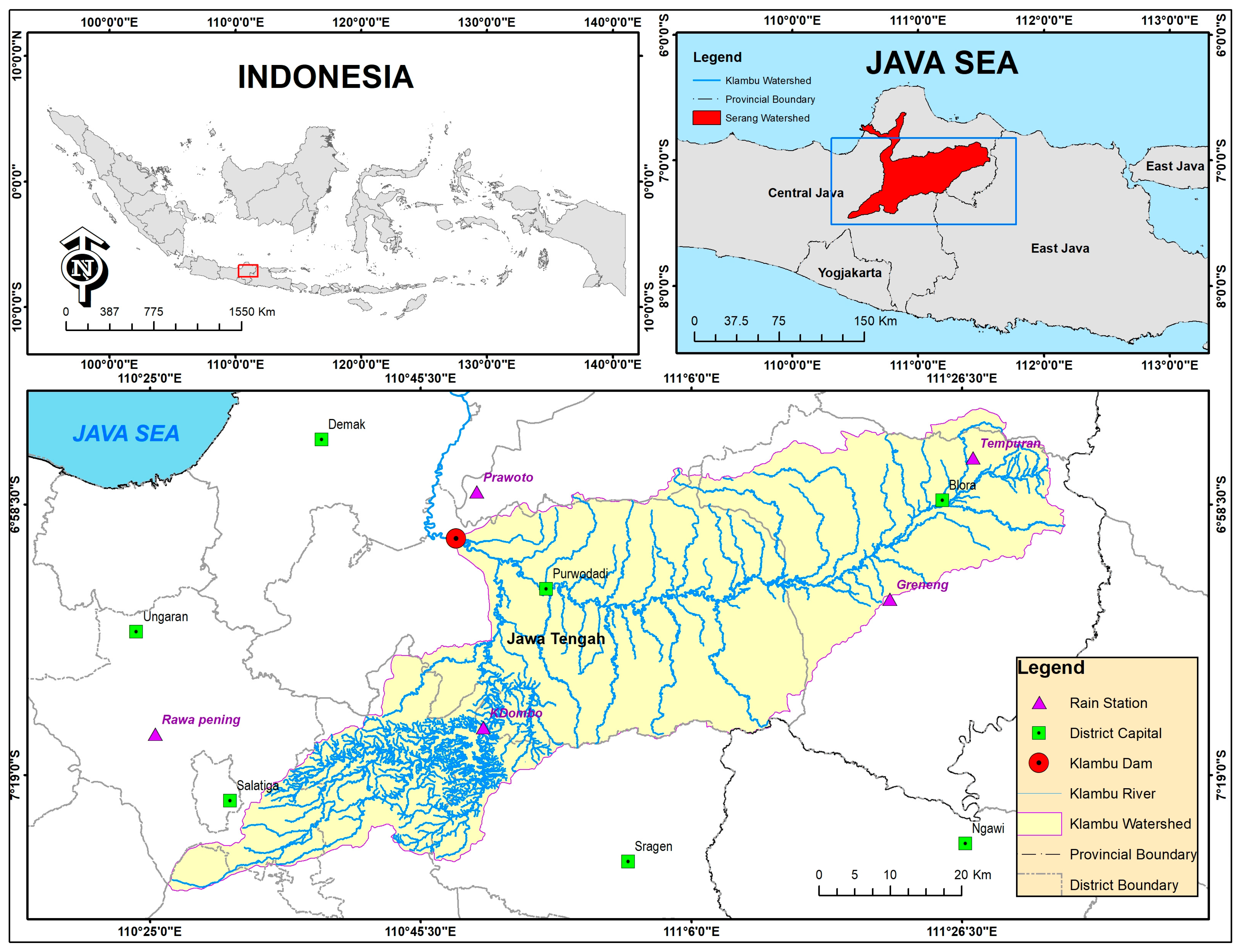
Figure 1. Research Location on Klambu Dam Catchment Area.
Water 18 00250 g001
Figure 2. Land Cover Change on Klambu dam Catchment Area.
Water 18 00250 g002
Figure 3. Methodological framework for this study.
Water 18 00250 g003
Figure 4. Average annual air temperature and average annual precipitation in 2000–2023.
Water 18 00250 g004
Figure 5. Distribution of average monthly air temperature and average precipitation totals for the 2000–2023 multi-year period.
Water 18 00250 g005
Figure 6. Distribution of precipitation totals during the year in 2000–2023.
Water 18 00250 g006
Figure 7. Trend Dynamics of Land Cover Change from 2000–2040.
Water 18 00250 g007
Figure 8. Land Cover Simulation in 2030 and 2040.
Water 18 00250 g008
Table 1. Ground Data Recap Research Availability of Kiambu Dam.
TypeStationElevation
(msl)
Research Data
(Years)
Temporal
Data
Quality
Missing Data
(Number Of Years)
RainfallRawa Pening358.262000, 2005, 2010, 2015, 202040%2000, 2005 and 2020
RainfallKedung Ombo358.262000, 2005, 2010, 2015, 20200%2000, 2005, 2010, 2015 and 2020
RainfallPrawoto110.12000, 2005, 2010, 2015, 202020%2000, 2005, 2010 and 2020
RainfallTempuran98.22000, 2005, 2010, 2015, 202020%2000, 2005, 2010 and 2015
RainfallBKSDA B SOLO358.262000, 2005, 2010, 2015, 202080%2000
RainfallGreneng98.22000, 2005, 2010, 2015, 202020%2000, 2005, 2010 and 2015
TemperaturesSemarang/Salatiga2832000, 2005, 2010, 2015, 202040%2000, 2005 and 2010
TemperaturesUngaran358.262000, 2005, 2010, 2015, 202040%2000, 2005 and 2010
TemperaturesPati98.22000, 2005, 2010, 2015, 202040%2000, 2005 and 2010
TemperaturesPurwodadi/Grobogan572000, 2005, 2010, 2015, 202040%2000, 2005 and 2010
DischargeKlambu DAM572000, 2005, 2010, 2015, 202033%2000, Feb & Sep 2005, and May–Oct 2015
Table 2. Observed Data (Precipitation-ΣP, Temperatures- Tav, and Discharge -ΣQ) of Klambu Dam.
ParametersJanFebMarAprMayJunJulAugSepOctNovDec
2005
ΣP (mm)229.7244.8321.4253.3101.0232.568.951.3113.0185.3219.1275.5
Tav (°C)27.928.028.328.028.828.427.928.328.628.828.427.7
ΣQ (m3)143.8117.290.6173.318.933.620.613.918.222.643.9107.4
2010
ΣP (mm)354.0280.6362.2166.8181.6103.095.683.8317.6199.2203.4297.0
Tav (°C)28.228.428.828.228.027.727.828.828.028.027.926.9
ΣQ (m3)106.494.2103.380.0116.842.017.616.552.762.668.1160.2
2015
ΣP (mm)261.3430.9342.9327.2119.731.56.312.42.929.2233.0266.8
Tav (°C)27.728.328.428.628.728.428.829.128.828.028.328.1
ΣQ (m3)114.9145.2145.2204.8134.112.912.412.913.410.941.0138.8
2020
ΣP (mm)339.7429.3352.4227.5188.934.6110.449.278.2163.6249.8411.5
Tav (°C)28.027.828.528.928.328.327.627.628.428.028.927.6
ΣQ (m3)131.9205.684.2154.311.414.214.214.114.03.368.0229.1
Table 3. Land Cover Series Data of Klambu dam catchment (in km2).
NoLand Cover200020052010201520202023
1Water Body51.824.237.155.228.439.5
2Forest523.2422.8634.1408.2107.5137.2
3Rice Field1091.71122.7442.9997.71034.21014.1
4Dry Agriculture748.2503.01045.8627.71217.3807.4
5Open Land16.760.887.046.041.364.3
6Built Area497.0209.7374.5436.8167.0319.0
7Diversified Farm117.0702.5424.3474.1449.9664.4
Sums3045.73045.73045.73045.73045.73045.7
Table 4. Comparison Results Between Observed Discharge and Calculated Discharge.
YearsDischarge (m3·s−1)Pearson
2005Q TWM8.370.644661
Q Obs66.99
2010Q TWM126.010.702479
Q Obs76.70
2015Q TWM93.520.943908
Q Obs82.22
2020Q TWM67.050.572959
Q Obs78.68
Table 5. Detailed Monthly Discharge Results from the Thornthwaite–Mather Model under C1/C2 Scenarios (2015).
ParametersJanFebMarAprMayJunJulAugSepOctNovDec
P (mm)339.71387.61330.04266.44152.9759.9743.4444.2380.15167.07219.1275.5
T (°C)27.9228.2028.5628.6228.4828.4828.3629.1029.2429.4028.2627.61
Lat−7.20−7.20−7.20−7.20−7.20−7.20−7.20−7.20−7.20−7.20−7.20−7.20
Rad−0.13−0.13−0.13−0.13−0.13−0.13−0.13−0.13−0.13−0.13−0.13−0.13
I354.0280.6362.2166.8181.6103.095.683.8317.6199.2203.4297.0
ƩI28.228.428.828.228.027.727.828.828.028.027.926.9
a4.504.504.504.504.504.504.504.504.504.504.504.50
f1.070.951.041.001.020.991.021.031.001.051.031.06
EP159.35166.70176.51178.08174.44174.21174.13191.95196.11201.23168.29151.66
Epx170.32158.38183.57178.08------173.33160.75
P-EP cor169.39220.23146.4788.36−24.96−112.50−131.11−153.48−115.96−44.22238.6693.45
surplus170.32158.38183.57178.08------173.33160.75
Deficit0.000.000.000.00−24.96−112.50−131.11−153.48−115.96−44.220.000.00
WHC/STO138.76138.76138.76138.76138.76138.76138.76138.76138.76138.76138.76138.76
e = 2.71828182842.722.722.722.722.722.722.722.722.722.722.722.72
S/D170.32158.38183.57178.08−24.96−112.50−131.11−153.48−115.96−44.222173.33160.75
APWL0.000.000.000.00−24.96−137.46−268.57−422.05−538.01−582.240.000.00
ΔSt138.76138.76138.76138.76129.5888.1939.96−16.50−59.16−75.43138.76138.76
EA170.32158.38183.57178.08282.55148.1683.3927.7320.9891.64173.33160.75
RO191.26201.94215.03224.86143.0059.6324.8710.374.321.8082.94158.72
Note: Explanations: P—precipitation (mm), T—air temperature (°C), Lat—latitude, I—effective precipitation, a—empirical coefficient based on temperature, f—day length correction factor based on latitude.
Table 6. Comparative Discharge Summary of the Thornthwaite–Mather Model under C1/C2 Scenarios for Selected Years.
YearsJanFebMarAprMayJunJulAugSepOctNovDecPearson
2000191.26201.94215.03224.86143.0059.6324.8710.374.321.8082.94158.720.952
2005148.67154.66160.30166.34105.9944.2018.437.693.2073.09137.31154.620.854
2010169.43182.04184.68185.37182.47114.0447.5519.8370.92131.11159.00164.480.802
2015194.49202.26213.21222.40141.8159.1424.6610.284.291.7983.19165.320.951
2020196.25199.89210.15225.35227.74143.1459.6924.8910.384.3393.21168.480.886
2030203.41188.62205.81223.74143.1659.7024.8910.384.331.8196.01190.980.947
2040237.77218.91239.86161.5267.3528.0911.714.882.040.85112.68224.780.812
Note: Explanations: The wet season (Blue marker), dry season (Orange Marker).
Table 7. Wet/Dry Month Dynamics Result of Thornthwaite-Matter method for each Scenario.
YearsJanFebMarAprMayJunJulAugSepOctNovDec
Scenario C 3, 4
2025wetwetwetwetdrydrydrydrydrydrywetwet
2030wetwetwetdrydrydrydrydrydrydrywetwet
2035wetwetwetdrydrydrydrydrydrydrywetwet
2040wetwetdrydrydrydrydrydrydrydrydrywet
Scenario C 5
2025wetwetwetwetdrydrydrydrydrydrywetwet
2030wetwetwetdrydrydrydrydrydrydrywetwet
2035wetwetwetdrydrydrydrydrydrydrywetwet
2040wetwetdrydrydrydrydrydrydrydrydrywet
Scenario C 6
2025wetwetwetwetdrydrydrydrydrydrywetWet
2030wetwetwetdrydrydrydrydrydrydrywetwet
2035wetwetdrydrydrydrydrydrydrydrydryWet
2040wetwetdrydrydrydrydrydrydrydrydrywet
Scenario C 7, 8
2025wetwetwetwetdrydrydrydrydrydrywetwet
2030wetwetwetdrydrydrydrydrydrydrydrywet
2035wetwetdrydrydrydrydrydrydrydrydrydry
2040drywetdrydrydrydrydrydrydrydrydrydry
Note: Explanations: The wet season (Blue marker), dry season (Orange Marker).
Disclaimer/Publisher’s Note: The statements, opinions and data contained in all publications are solely those of the individual author(s) and contributor(s) and not of MDPI and/or the editor(s). MDPI and/or the editor(s) disclaim responsibility for any injury to people or property resulting from any ideas, methods, instructions or products referred to in the content.