Article

Assessment of the Ecological Quality of the Santos Estuarine Complex (SE Brazil): Predictive Models and Benthic Foraminifera-Based Index


by
Silvia Helena de Mello e Sousa
1,*,
Bruno V. Damasio
1,
Carla Bonetti
2,
Felipe R. dos Santos
1,
Eduardo Siegle
1,
Cintia Yamashita
1,
Júlia Sambugaro
1,
Beatriz Saito
1,
Maria Virginia Alves Martins
3,4,
Rubens Cesar Lopes Figueira
1 and
Márcia C. Bícego
1
1
Instituto Oceanográfico, Universidade de São Paulo, Praça do Oceanográfico, 191, Cidade Universitária, São Paulo 05508-120, SP, Brazil
2
Laboratório de Oceanografia Costeira, Coordenadoria de Oceanografia, Universidade Federal de Santa Catarina–UFSC, Florianópolis 88036-020, SC, Brazil
3
Faculdade de Geologia, Universidade do Estado do Rio de Janeiro, UERJ, Av. São Francisco Xavier, 24, Sala 2020A, Maracanã, Rio de Janeiro 20550-013, RJ, Brazil
4
GeoBioTec, Departamento de Geociências, Universidade de Aveiro, Campus de Santiago, 3810-193 Aveiro, Portugal
*
Author to whom correspondence should be addressed.
Water 2026, 18(2), 172; https://doi.org/10.3390/w18020172
Submission received: 14 November 2025 / Revised: 21 December 2025 / Accepted: 3 January 2026 / Published: 8 January 2026

Abstract

The Santos Estuarine System, one of the most anthropogenically impacted coastal regions in Brazil, was studied using benthic foraminiferal assemblages to determine four distinct stages of organic pollution. Predictive models combined with the Ecological Quality Status (EcoQs) index were applied to relate pollution stages to abiotic parameters (total organic carbon, mud content, and salinity variability) and organic contaminants, including aliphatic (AHs) and aromatic hydrocarbons (PAHs), linear alkylbenzenes (LABs), and coprostanol. The pollution gradient ranged from low (São Vicente Channel and Santos Bay, characterized by Ammonia tepida and medium coprostanol concentrations), to moderate (Santos Channel, with Bulimina elongata and Triloculina sp.1), high (Bertioga Channel, showing Cribroelphidium poeyanum, Paratrochammina sp.1, high levels of LABs, and TOC), and severe (Upper Estuary, marked by Ammonia sp.1 and high concentrations of PAHs and coprostanol). A linear discriminant analysis (LDA) demonstrated an overall accuracy of 70%, suggesting that the discriminant model performs reasonably well in predicting the predictive ability of foraminifera species to distinguish between areas with varying pollution status based on organic pollutants. Also, the potential use of the EcoQs index in assessing the environmental quality of a subtropical estuary subjected to organic pollution was demonstrated.

1. Introduction

Coastal regions, encompassing major metropolitan areas, support a substantial proportion of the global population, with approximately 29% residing within 50 km of the coastline and 15% within 10 km [1], rendering these ecosystems among the most heavily impacted and ecologically vulnerable worldwide [2,3]. Although human activities in these regions are fundamental for the healthy economy of countries, they are responsible for causing severe social and environmental problems, such as conflicts of use in coastal lands, mass tourism, and structural engineering works (piers, dikes, spikes, breakwaters, jetties, etc.), which can cause changes in sedimentary dynamics, saltwater intrusion, entailing coastal erosion and subsidence [4,5,6,7].
In addition, the anthropogenic activities in coastal metropolises release a wide range of pollutants into the marine environment, such as trace metals, persistent organic pollutants (POPs), polycyclic aromatic hydrocarbons (PAHs), halogenated and aromatic solvents, automotive fuels, antifouling biocides, antibiotics and other drugs for human and veterinary use, hygiene and personal care products, hormones, illicit drugs, among others [8,9,10,11,12,13,14,15]. The Santos, São Vicente, and Bertioga Estuarine System (hereinafter, the Santos Estuarine System), situated in a coastal Brazilian region with approximately 1.5 million inhabitants [16], which may increase significantly during the holiday season due to a large influx of tourists, is one of Brazil’s most prominent examples of environmental degradation [17]. Besides the urban activities, this estuarine system houses the largest port in Latin America (Port of Santos) and the country’s largest industrial hub in Cubatão [18] which have transformed the estuary into a significant sink for pollutants, a process initiated with the opening of the Port of Santos in 1892 and intensified by industrial expansion in the 1950s [19] (Figure 1). Although environmental conditions have improved in recent decades due to the control of pollutant sources by the Environmental Company of the State of São Paulo (CETESB), research has detected considerable metal concentrations in sediments, such as in the port region of Santos and near the Cubatão industrial complex [19]. Also, hydrocarbon analysis showed widespread contamination on the estuary, with higher concentrations in the Piaçaguera River, decreasing towards the Santos channel [20].
Benthic foraminifera (amoeboid protists) have shown remarkable potential as bioindicators for assessing environmental quality and conducting biomonitoring in marine, coastal, and transitional environments [21,22,23,24,25]. Their effectiveness is related to their abundance and distribution in modern oceans (e.g., [26]), key biogeochemical roles in carbon and nitrogen cycling (e.g., [27]), and short reproductive and life cycles, allowing rapid responses to environmental changes (e.g., [23,28]). Consequently, species differ in their tolerance to environmental stress [29,30,31], and their relation may be used to infer pollution status.
Recent advances in benthic foraminiferal biotic indices (see [32], for a review) have expanded the potential for using this group as a biological quality element in the Ecological Quality Status (EcoQs) assessment of marine and transitional water environments in Brazil (see [23], for a review). One of these indices is based on species diversity (i.e., [33]) that has been successfully applied to assess the EcoQs of several environments (e.g., [25,32,34,35,36,37,38,39,40]). Some studies have already described the distribution of the foraminifera fauna in the Santos Estuarine System [41,42,43,44,45]. However, none of them focused on analyzing benthic foraminifera to assess the ecological quality of the estuary using biotic indices.
Considering the above, the present work aims: (a) to evaluate the quality status of the Santos Estuarine System based on organic pollutants, considered with a widespread distribution in the system; (b) to establish a predictive model to be applied in monitoring studies; and (c) to evaluate the use of Ecological Quality Status index based on living benthic foraminifera to assess the state of health of the superficial bottom sediments of the Santos Estuarine System. Furthermore, this study’s results will provide environmental regulatory agencies with an evidence-based system management framework.

Study Area

The Santos Estuarine System (between 23°51′ S–24°02′ S and 46°17′ W–46°28′ W) is located in the São Paulo State, Brazil. It encompasses the municipalities of Praia Grande, São Vicente, Santos, Cubatão, Guarujá, and Bertioga (Figure 1).
The Santos Estuarine System comprises the Santos Bay, a complex tangle of rivers (e.g., Perequê, Onça, Piaçaguera, Jurubatuba, Diana, Bertioga, and Santana, among others), and several channels, such as Bertioga, Barreiros, Piaçaguera, Mar Pequeno, and the Pompeba, Candinho, São Vicente, and Santa Rita squares [46]. The region can be divided into four large compartments according to the hydrodynamic pattern: Santos Bay, Santos Channel (Port Channel), São Vicente Channel, and Bertioga Channel [47]. The estuarine system is affected by semidiurnal tidal waves, with average amplitudes varying between 0.27 m (neap tide) and 1.23 m (spring tide) [48]. According to Harari et al. [49], the upper Santos estuary region is influenced by the rivers that flow into the area, the Serra do Mar, the tide, and the waters from the Bertioga channel. These rivers generate a unidirectional surface flow that propagates towards Santos Bay.
The Santos Port Channel generally presented the highest velocities of the entire domain. In the region close to its mouth, velocities reached 1.4 m s−1 during spring tide and up to 0.7 m s−1 during neap tide. During neap tides, velocities in the main channels (excluding regions near the mouths) reach approximately 0.4 m s−1. During spring tides, velocities are stronger and exhibit greater spatial variability, reaching approximately 1.2 m s−1 [50].
The flood currents dominate the Santos channel, while ebb currents dominate the São Vicente and Bertioga channels. The strongest currents were observed in the Santos Channel. It was also shown that the influence of river flow and channel morphology creates sub-regions with different hydrodynamic behaviors within the same estuarine channel. Also, Damasio et al. [20] presented a model showing that suspended particles are driven into the estuary and, on average, are deposited at the mouth of the Bertioga Channel and the Santos Channel [51].
The estuary exhibits substantial temporal variation in salinity, driven by the tidal cycle and changes in freshwater discharge. According to Harari et al. [52], salinity varies spatially from 15 to 35 in the Santos estuary, with vertical variations showing an increase in salinity with depth up to 4. A similar vertical stratification was observed in the Piaçaguera Channel [53]. Freshwater enters the estuary mainly in the middle and upper regions of the estuary, where the mangroves are present, mainly through the rivers Itatinga (~12 m3 s−1), Itapanhaú (~10 m3 s−1), Cubatão (~5 m3 s−1), Quilombo (~5 m3 s−1), Boturaca (~4 m3 s−1), and Jurubatuba (~4 m3 s−1) [54].
The study area alternates between tropical and polar Atlantic systems, with a hot, humid tropical climate, no defined dry season, and average temperatures above 20 °C. Annual rainfall ranges from 2000 to 3000 mm, and the average relative humidity is nearly 85% [55]. The sediment is predominantly fine, ranging from silt to very fine sand, characterizing the estuary as a low-energy sedimentation environment with low flocculation rates [56].

2. Materials and Methods

2.1. Sediment Sampling

Three surface sediment sampling campaigns were conducted during the austral winter and spring of 2019 in the Santos Estuarine System, each targeting a specific region within the system: the São Vicente Channel (SV), the Santos Upper Estuary, Channel and Bay (S), and the Bertioga Channel (B). In total, 21 stations were established across the three areas (SV = 5, S = 11, B = 5) (Figure 1). In the Supplementary Materials, S1 provides detailed information on the sampling dates, coordinates (Datum SIRGAS 2000), locations, water depths, and vessels employed.
Because of the shallow depths in the Bertioga and São Vicente channels, cores were manually collected during the first and third campaigns by inserting acrylic tubes directly into the sediments. This method allowed the recovery of undisturbed surface sediments for the analysis of living benthic foraminifera. In the second campaign, a multiple corer was used. At each station, three 8 cm diameter cores were taken from distinct deployments. This follows the recommendation that three replicates per station are necessary to capture small-scale spatial variability in benthic foraminiferal distribution [28,57].
The core was subsampled using an extruder, and the first centimeter of sediment was sliced and stored in plastic bottles. A solution of 2 g of rose Bengal and 1 L of ethanol (90%) was added to differentiate living (stained) from dead foraminifera [58,59]. The samples were stored in a refrigerator for at least 14 days to ensure proper staining of living foraminifera [28]. Only individuals with all chambers stained pink (except the last chamber) were considered alive.
In addition, surface sediment samples were also collected using a stainless steel van Veen bottom grab for sedimentological and elemental (total organic carbon—TOC and carbonate content) analysis as well as for the determination of the organic compounds, including polycyclic aromatic hydrocarbons (PAHs), aliphatic hydrocarbons (AHs), linear alkylbenzenes (LABs), and fecal sterols, using aluminum foils previously cleaned and calcined in a muffle oven at 450 °C.

2.2. Laboratory Procedures

A total of 63 sediment samples (triplicates from 21 stations) were analyzed for benthic foraminifera. Each sample (50 cm3 of wet sediment) was washed through a 63 μm sieve, oven-dried at 40 °C, and the resulting >63 μm fraction was examined. At least 100 foraminifera tests per sample were analyzed, following the recommendations of Schönfeld et al. [28] and Fatela & Taborda [60]. The results from the three replicates were averaged to obtain a single representative value for each station.
The identification of genus and species followed the classification made by [20,43,61,62,63,64] under a SMZ800N stereomicroscope (Nikon Instruments Inc., New York, NY, USA). Species names were updated according to the World Register of Marine Species (WORMS) [65]. Some photos of the species found were taken on the ZEISS SteREO Discovery.V20 stereomicroscope (Carl Zeiss AG, Oberkochen, Germany) using the ZEN 2012 Imaging Software version 1.1.2.0 (Plate 1).
Grain-size and organic contaminant analyses were performed on one surface sediment sample (one replicate) from each of the 21 stations.
The grain-size analysis was performed according to the methodology described by Suguio [66].
The TOC determination used a modified Walkley & Black [67] method, based on the oxidation of organic carbon with potassium dichromate and sulfuric acid, followed by titration with ferrous ammonia sulfate. Three sediment aliquots and three blanks per station were analyzed, and the mean TOC value was calculated for statistical analyses.
The procedure for determining organic contaminants was based on [68,69,70]. It consisted of extracting 10 g of sediment in Soxhlet with 80 mL of a mixture of dichloromethane/n-hexane (1:1 v/v) for 8 h after adding surrogate standards. The following were used as surrogate standards: n-Hexadecene for aliphatic hydrocarbons (AHs); 1-C12-LAB for linear alkylbenzenes (LABs); d8-naphthalene, d10-acenaphthene, d10-phenanthrene, d12-chrysene, and d12-perylene for polycyclic aromatic hydrocarbons (PAHs); and 5α-androstanol for sterols.
After extraction, the samples’ purification and fractionation were carried out via liquid-solid adsorption chromatography in an open glass column filled with 3.2 g of alumina (5% water deactivated) and sodium sulfate (Na2SO4). AHs, PAHs, and LABs were eluted with 20 mL of 30% dichloromethane/hexane mixture (7:3, v/v; Fraction 1 (F1)), while sterols were eluted with 20 mL of methanol/dichloromethane mixture (1:1, v/v; Fraction 2 (F2)).
Internal standards (n-tetradecene for AHs; p-terphenyl for HPAs, and 1C19-LAB for linear alkylbenzenes) were added to the F1 extracts. F1 was injected into a gas chromatograph (GC, Agilent 6890) (Agilent Technologies Inc., Santa Clara, CA, USA) coupled to a flame ionization detector (FID) for AHs quantification. F1 was also injected into a gas chromatograph (GC, Agilent 7010B) connected to a triple quadrupole mass spectrometer (MS/MS) operating in multiple reaction monitoring (MRM) for PAHs and LABs quantification.
The F2 extracts were dried and derivatized with BSTFA (bis (trimethylsilyl) trifluoroacetamide) and 1% TMCS (trimethylchlorosilane) for 90 min at 65 °C. After derivatization, the internal standard (5α-cholestane) was added, and the extracts were injected into GC-FID for sterols quantification.

2.2.1. Hydrodynamic Modeling of Bottom Water Salinity

Based on benthic foraminifera analysis performed by Bonetti [42] and Debenay et al. [43], the salinity is a controlling factor in the benthic foraminifera distribution in the Santos Estuarine System. However, during the sampling, salinity values were not measured. Therefore, to obtain the minimum, maximum, and average variation in bottom water salinity, instead of instantaneous salinity measurements at the sampling stations, the three-dimensional Delft3D hydrodynamic model for the Santos Estuarine System, applied and validated by Seiler et al. [51], was used for the stations defined in this study.
The domain of the numerical model covers the entire estuarine system and the adjacent oceanic region. The numerical grid used is curvilinear and includes, as boundary conditions, river discharge from rivers flowing into the estuary, water-level variation at the oceanic boundary, and corresponding salinity values. The three-dimensional model was defined with 12 vertical layers (z-layers) of varying thickness from the surface to the bottom. For further details on the model application and its validation, see Seiler et al. [51].
The present application used the model results extracted in July 2014, the same period used for the model validation [51]. The results were extracted for each station from its bottom-most layer. From the modeled bottom salinity time series, the maximum and minimum salinity values were defined, and thus the degree of variation at each point.

2.2.2. Biotic Environmental Indices

The EcoQS (Table 1; [33]) was calculated using the RStudio software version 4.5.1 [71] and the Entropy Library version 1.2./1 [72]. The EcoQS limits adapted to transition regions were applied (Table 1; [34]). This index is the exponential of the bias-corrected Shannon Index [73].

2.3. Multivariate Analysis

Given that the entire study area is subject to organic pollution [20], a K-means analysis was employed to delineate groups of sites with comparable concentrations of organic compounds. The dataset encompassed six sediment quality variables: TOC, AHs, PAHs, LABs, coprostanol, and unresolved complex mixture/resolved aliphatics ratio (UCM/ResAHs). A correlation-based distance matrix was computed from standardized, log-transformed data (n = 21 samples). Statistical differences among the identified groups were assessed using the Kruskal–Wallis median test, with subsequent Dunn post hoc testing performed when the null hypothesis of equality (H0) was rejected. Data analysis was conducted using the FactoMineR package version 2.12 [74].
The predefined site groups, distinguished by their associations with organic contaminant descriptors, were used as the categorical response variable in a linear LDA. This analysis assessed the predictive ability of foraminifera species to distinguish between areas with varying pollution status (low, moderate, high, and severe). Data preprocessing for the LDA model involved excluding taxa that contributed less than 0.5% of the total community abundance and occurred in less than 20% of the samples. This analysis resulted in a dataset of 9 foraminifera species from 63 samples (21 sites, each with three replicates). The predictor species utilized in this analysis included: Ammonia parkinsoniana, Ammonia tepida, Ammonia sp.1, Bolivina striatula, Bulimina elongata, Cribroelphidium excavatum, Cribroelphidium poeyanum, Paratrochammina sp.1, and Triloculina sp.1. Relative abundance values were log-transformed (log10 x + 1) before analysis. The model assumed that group probabilities were proportional to sample sizes (prior probabilities). The coefficients of linear discriminants were used to measure the importance of each input variable in discriminating between the groups. Leave-one-out cross-validation (jackknifing) was employed to assess the model’s predictive power, with performance metrics (accuracy, sensitivity, specificity) evaluated using a confusion matrix. The LDA model was fitted using the MASS R package version 7.3.65 [75], and all plots were generated using the ggplot2 package version 3.5.2 [76].
To identify which species, among those used in the LDA model, served as the best indicators for each environmental group, the Indicator Value (IndVal) index was applied [77]. This analysis calculates indicator taxa for each group based on their relative abundance and fidelity (proportion of occurrences within a group). This study used a threshold of ≥35% IndVal and a p-value < 0.05 to identify statistically significant indicator species. The analysis was performed using the labdsv package version 2.1-0 [78].
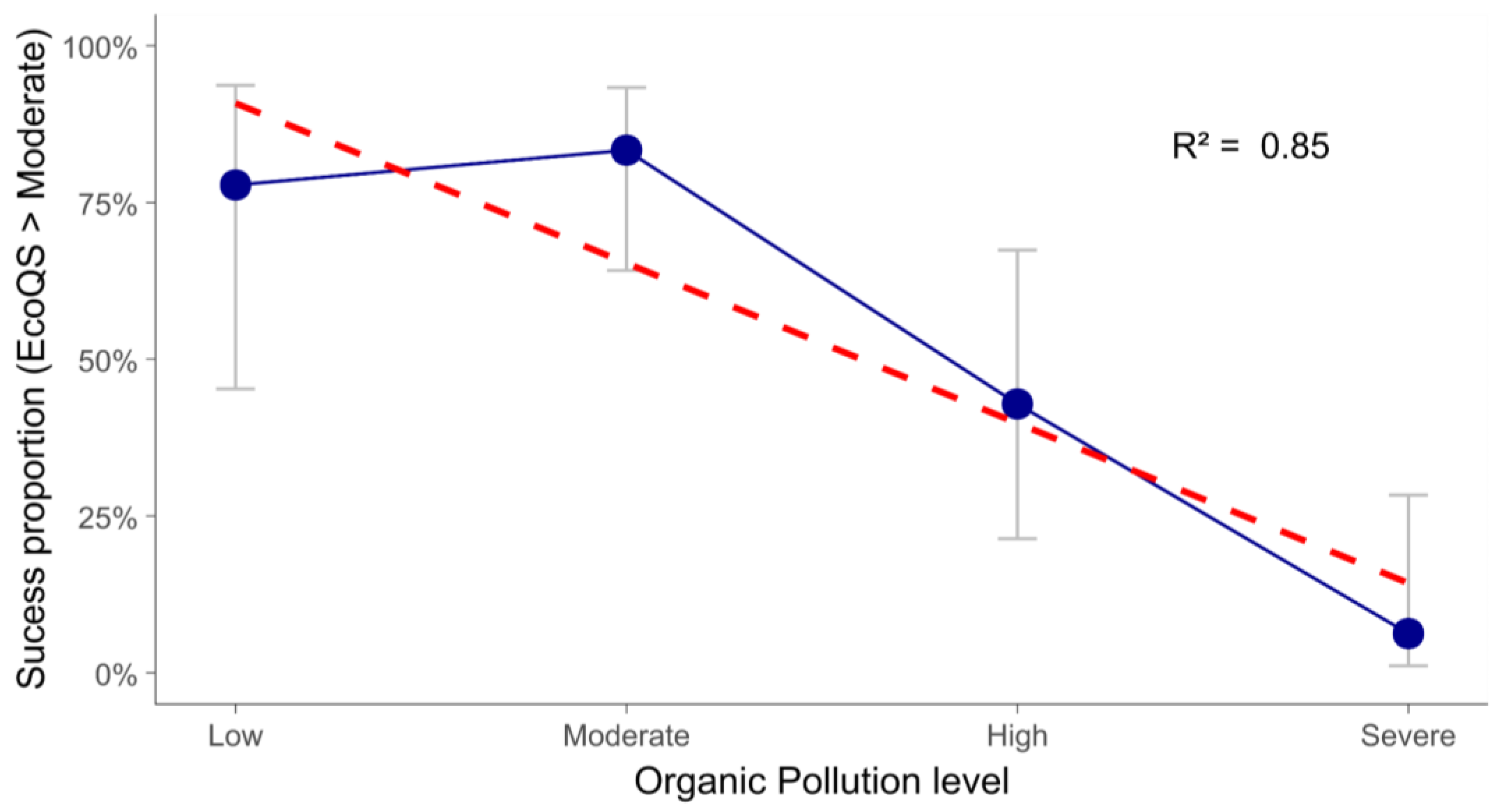
To assess the association between EcoQS (ordinal categories: Poor, Bad, Moderate, Good, Excellent) and organic pollution levels (ordinal categories), contingency tables were constructed and tested for independence using Fisher’s exact test. The strength and direction of association were quantified using Goodman–Kruskal’s gamma. An ordinal logistic regression model was fitted to evaluate the relationship between EcoQS and OrgPoll. The model was implemented with the polr function in the MASS package, with EcoQS as the ordered response variable (levels from “Poor” to “Excellent”) and OrgPoll as the ordered predictor. Model fit and significance were assessed using the Likelihood Ratio Test, and explanatory power was evaluated using McFadden’s Pseudo-R2. Additionally, EcoQS was transformed into a binary variable (≥Moderate and <Moderate categories) to test for a monotonic relationship across pollution levels using the Cochran-Armitage trend test. Finally, the proportion of “success” cases (EcoQS ≥ Moderate) was plotted across pollution categories with 95% confidence intervals (Wilson method), and a linear trend line was added to illustrate the direction of the association.

3. Results

3.1. Environmental Variables

The values of the environmental variables are presented in Table 2. The percentage of fine sediments varied between 6.45% and 98.46% in the Santos Estuary System (stations S11 and B2, respectively). Generally, the Bertioga Channel, the Upper Estuary, and the northern part of the Santos Channel presented a high percentage of fine sediments. In contrast, the São Vicente Channel, the southern part of the Santos Channel (stations S9 and S10), and Santos Bay presented coarser sediments. The exceptions are station B5, in the Bertioga Channel, which presented 17.26% of fine sediments, and station SV4, in the São Vicente Channel, which presented 91.77% of fine sediments (Table 2, Supplementary Materials S2).
Regarding carbonate, there is a trend of higher values towards Santos Bay and lower values towards the Upper Estuary (Table 2). The values ranged from 0% (stations S1, S4, and B3) to 14.80% (station S7). In the Bertioga Channel, the average was 0.8%; in the São Vicente Channel, 3.08%; in the Upper Estuary, 3.27% and in the Santos Channel, 10.15%. The Santos Bay station presented 3.66% of CaCO3.
The TOC values (Table 2) ranged from 0.53% to 5.47% (stations S11 and B2, respectively). The Bertioga Channel presented the highest values throughout the estuary, with four stations above 4.5%. Station B5 was the exception, presenting only 0.87%. The São Vicente Channel presented intermediate values, ranging from 0.67% (stations SV1 and SV5) to 3.88% (station SV4). The Upper Estuary presented values ranging from 2.32 to 4.33% (stations S1 and S2, respectively). The Santos Channel, in turn, presented the lowest values in the estuary, with the highest at station S6 (2.35%) and gradually decreasing to station S10 (1.28%) (Table 2, Supplementary Materials S2).
The total AHs (ΣAHs), UCM, and UCM/Res varied from 5.9 to 321.7 µg g−1, from 1.62 to 272.28 µg g−1, and from 0.38 to 6.65, respectively, throughout the Estuarine System of Santos, São Vicente, and Bertioga. Sediments with ΣAHs < 10 μg g−1 are considered not contaminated, while ΣAHs > 100 µg g−1 are associated with petroleum inputs. When ΣAHs concentrations are <50 μg g−1, a more detailed analysis of the hydrocarbon constituents is required to assess the magnitude of contamination [79,80]. 47.6% of the samples showed ΣAHs > 100 µg g−1, while only 14.3% showed values < 10 µg g−1, suggesting that the Santos Estuarine System is under a high level of petroleum pollution. The Santos Upper Estuary stations (S1 to S4) showed the highest concentrations, followed by the Bertioga and São Vicente channels. UCM was detected in all samples, exhibiting higher concentrations and UCM/Re in the Cubatão Industrial Complex (samples S1 to S6), suggesting extensive biodegradation of petroleum-related inputs (UCM/Res > 4), while the rest of the samples suggested recent pollution that has been diluted by natural inputs [81,82,83] (Table 2, Supplementary Materials S2 and S3).
The total PAHs (ΣPAHs) and the Σ16PAHs varied from 104.5 to 22,374 ng g−1 and from 57.9 to 16,272 ng g−1, respectively. Baumard et al. [84] categorized parent PAH concentrations in sediments as low, moderate, high, and very high, corresponding to levels of 0–100, 100–1000, 1000–5000, and >5000 ng g−1, respectively. However, this definition focuses explicitly on Σ16PAHs and does not consider the alkyl-substituted PAHs, which could also play a significant role in the sources of fossil PAHs. On this basis, the Σ16PAH concentrations in the Estuarine System of Santos, São Vicente, and Bertioga indicated that 57.1% of the stations are classified as high, 28.8% as moderate, 14.3% as very high, and 4.8% as low. The spatial distributions of ΣPAHs and Σ16PAHs were similar to those of the aliphatic hydrocarbons, with higher concentrations occurring in the inner portions of the estuary (Table 2, Supplementary Materials S2 and S3).
Total LABs (ΣLABs) and coprostanol concentrations varied from 62.5 to 1382.8 ng g−1 and 0.11 to 4.66 µg g−1, respectively. ΣLABs showed higher values at SV4, S6, and S11, while cop showed the highest concentrations at SV4, S2, S4, and S11 (Table 2, Supplementary Materials S2 and S3). To the best of our knowledge, LABs are not classified by contamination levels in the literature. In this study, we considered the threshold concentration of coprostanol in uncontaminated sediments as ≤0.01 µg g−1 [85], contaminated sediment as ≥0.1 µg g−1 [86,87], and highly contaminated sediment as ≥ 0.5 µg g−1 [88].
The modeled Δ salinity values decreased from the Upper Estuary (up to 4.33) to Santos Bay (up to 1.5). The highest values are observed in the Bertioga Channel (up to 4.57) and in the São Vicente Channel (3.51; Table 2, Supplementary Materials S2 and S3).

3.2. Benthic Foraminifera Analysis

The most abundant taxa (relative abundance >1%) were Ammonia tepida, Ammonia sp.1, Ammonia spp., Bolivina striatula, Bulimina elongata, Cribroelphidium excavatum, Cribroelphidium poeyanum, Cribroelphidium spp., Nonionella spp., Paratrochammina sp.1, Paratrochammina spp., Quinqueloculina spp., Triloculina sp.1, and Trochammina spp. (Supplementary Materials S4 and S5).
In the Santos Upper Estuary, Ammonia sp.1 dominated the assemblages, accounting for 60.8% of the fauna, accompanied by Ammonia spp. (12.9%), Triloculina sp.1 (9.3%), and Ammonia parkinsoniana (6.6%), and another 30 taxa represent 10.5% of the assemblage. In the Santos Channel and Bay, Ammonia sp.1 accounts for 31.3% of the assemblage, and another taxa >5% relative abundance in this region are Triloculina sp1. (13.8%), Ammonia tepida (7.9%), and Ammonia spp. (7.7%).
In São Vicente Channel, assemblages were characterized by the co-occurrence of Ammonia sp.1 (25.4%) and Cribroelphidium excavatum (23.9%), with additional contributions from Cribroelphidium spp. (12.2%), Triloculina sp.1 (7.9%), and Ammonia spp. (5%). The Bertioga Channel was dominated by the agglutinant species Paratrochammina sp.1 (31.1%), along with Ammonia sp.1 (14.9%), Cribroelphidium excavatum (11.7%), Quinqueloculina spp. (7.9%), Trochammina spp. (5.6%), and Ammonia parkinsoniana (5.3%).
Applying Pearson correlation, significant correlation values between δ salinity values and the most abundant benthic foraminifera species were obtained, e.g., Paratrochammina sp.1 (0.6, p = 0.0026), Cribroelphidium excavatum (0.6, p = 0.0015), Cribroelphidium poeyanum (0.5, p = 0.0134), Quinqueloculina spp. (0.5, p = 0.0207), Nonionella spp. (−0.5, p = 0.0074), Bolivina striatula (−0.6, p = 0.0038), Bulimina elongata (−0.7, p = 0.0003).
Species richness demonstrated considerable variability, ranging from a minimum of 7 species at station S1b to a maximum of 27 species at station S10b. The density of living specimens ranges from 39 individuals per 50 cm3 at station SV2b to 3758 individuals per 50 cm3 at station S3c. The highest value (0.71) of the dominance index was recorded at S1a, while the lowest (0.06) at S10b. Shannon-Wiener diversity shows the lowest value (0.96) at S1a and the highest value (4.27) at S10b. Finally, Pielou’s Equitability followed the same trend, ranging from a minimum of 0.27 to a maximum of 0.92 (Supplementary Materials S6).

3.3. Statistical Analysis

3.3.1. Environmental Zoning Based on Geochemical Indicators of Organic Pollution

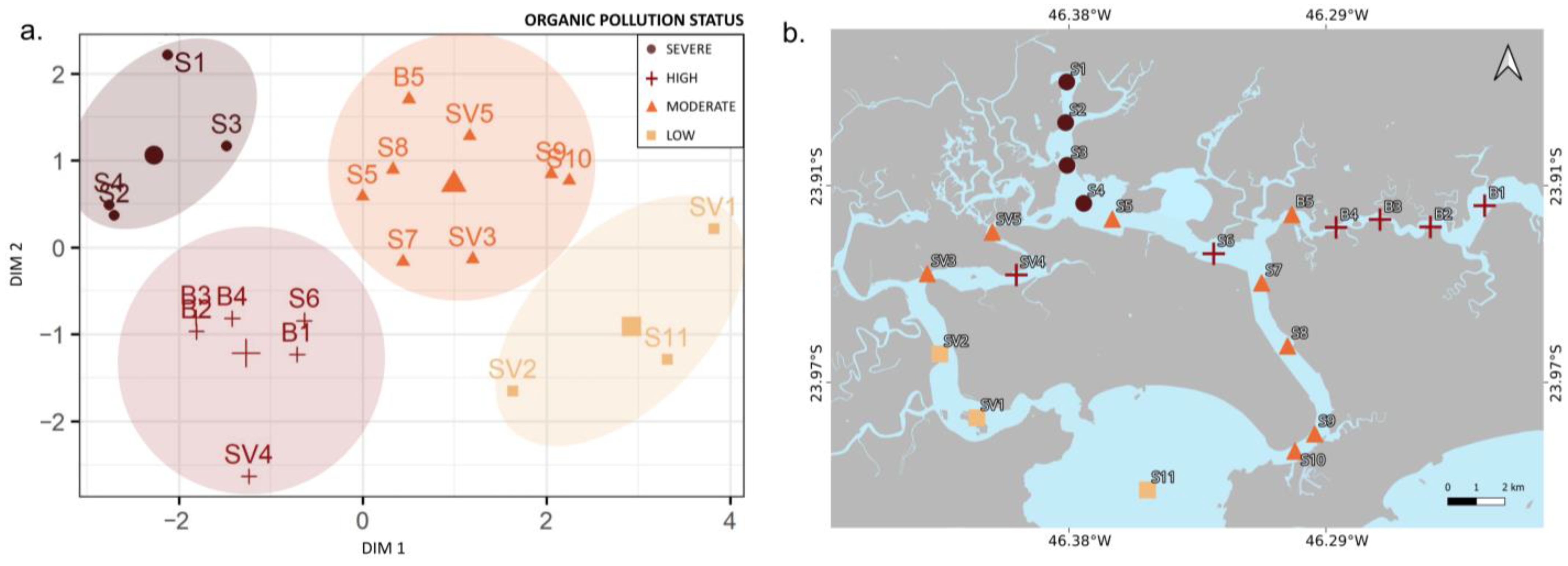
Using the K-means clustering algorithm, the study area was segmented into four distinct groups: low, moderate, high, and severely polluted zones (Figure 2a). These divisions correspond to the organic pollution gradient observed across the study area. The low pollution group consisted of three sites: one in Santos Bay and two in the São Vicente Estuary, closer to the inlet. Samples in the moderately polluted category encompassed eight sites along the lower Santos Estuary and the upper estuary of São Vicente. The high-pollution group (6 sites) was concentrated in the upper Santos Estuary and the Bertioga Channel. Finally, the severe pollution group (4 sites) was confined to a further inland location, along the Piaçaguera Channel (Figure 2b).
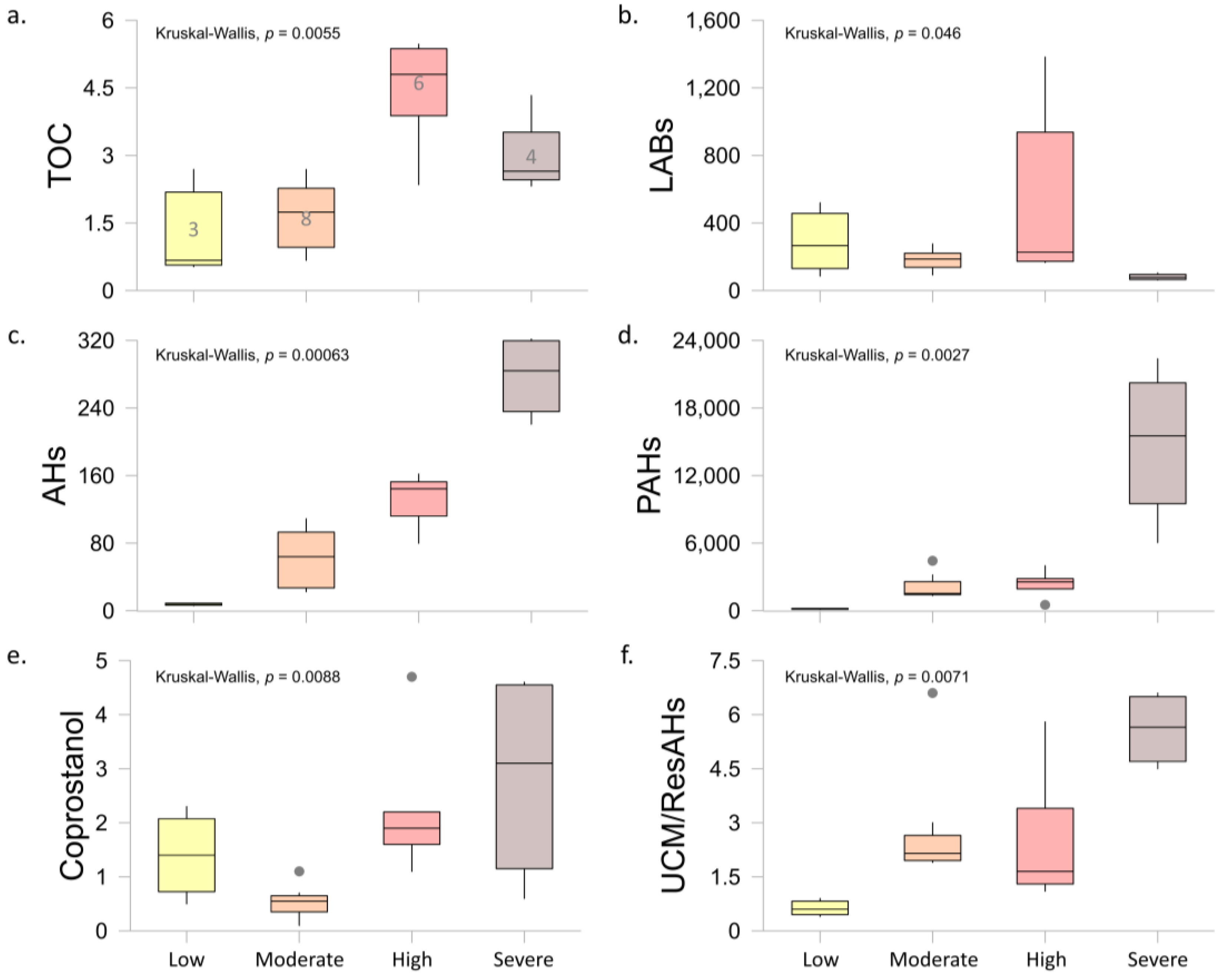
The pollution status of these K-means-based groups was determined by analyzing the medians and maximum concentrations of organic pollutants in their respective sediments, as depicted in Figure 3. Significant differences were observed among the groups for all organic variables (p-values for KW’s test < 0.05). Generally, there is a trend of increasing concentrations of TOC, AHs, PAHs, and UCM/ResAHs from the low to the severe group.
However, a notable exception to this gradient was observed in LABs, which exhibited the lowest concentrations (md = 77.9 ng g−1) in the severely polluted group. The other groups showed median concentrations ranging from 186.2 ng g−1 (moderate group) to 266.4 ng g−1 (low group).

3.3.2. Foraminifera Species as Predictors of Organic-Polluted Zones

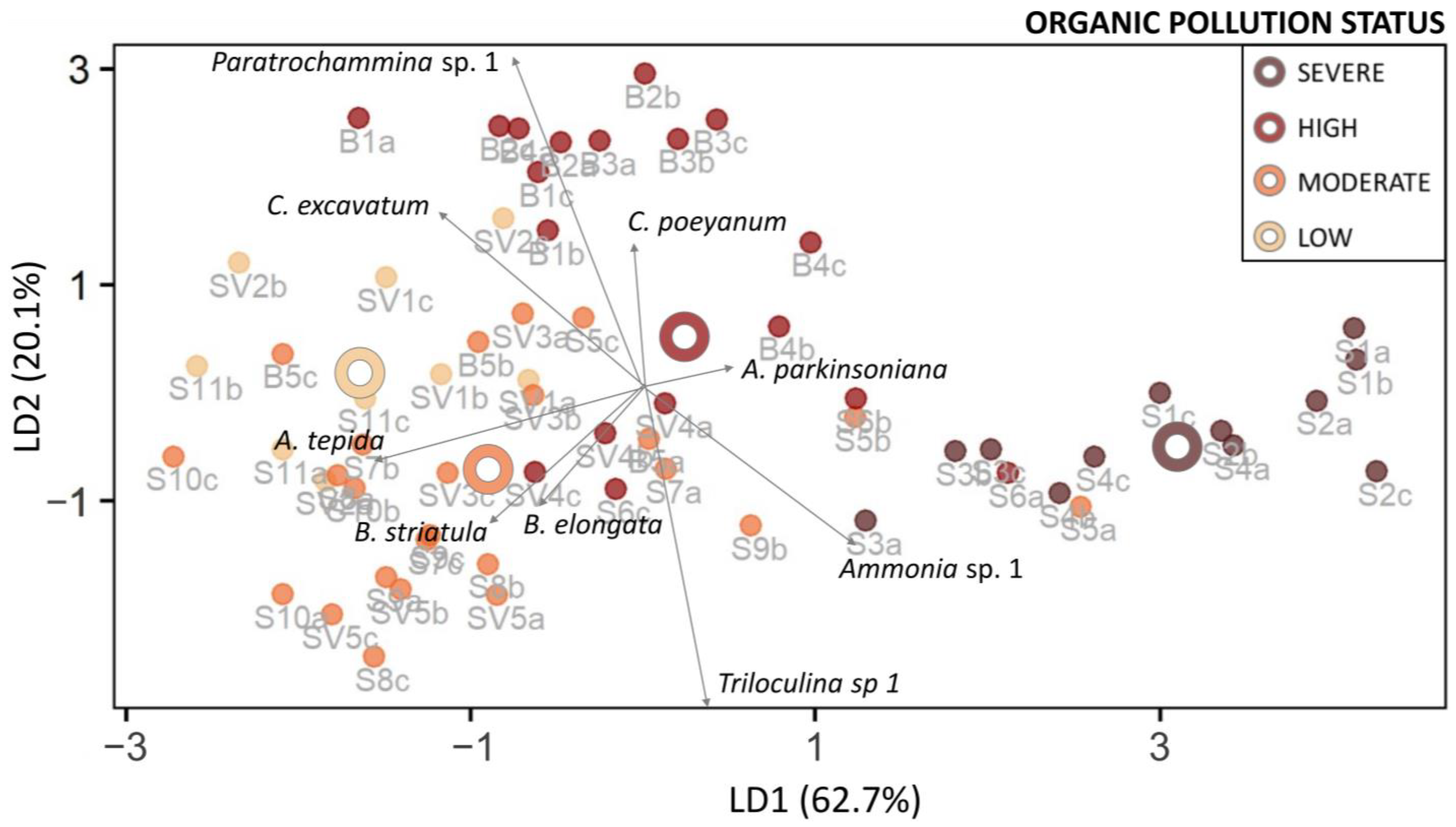
The linear discriminant analysis results supported the hypothesis that the four organic-polluted zones, as determined solely by organic descriptors, could also be distinguished based on the relative abundance of foraminifera species as predictors (Figure 4). The first and second linear discriminant (LD) functions explained 62.7% and 20.1% of the variance, respectively. Clear separation of group centroids was observed, primarily along the first LD axis, indicating differences among all groups, particularly pronounced between low- and severe-pollution zones. The contribution of each species to the LD function, as analyzed through the coefficients of linear discriminants, is depicted as vectors in Figure 4.
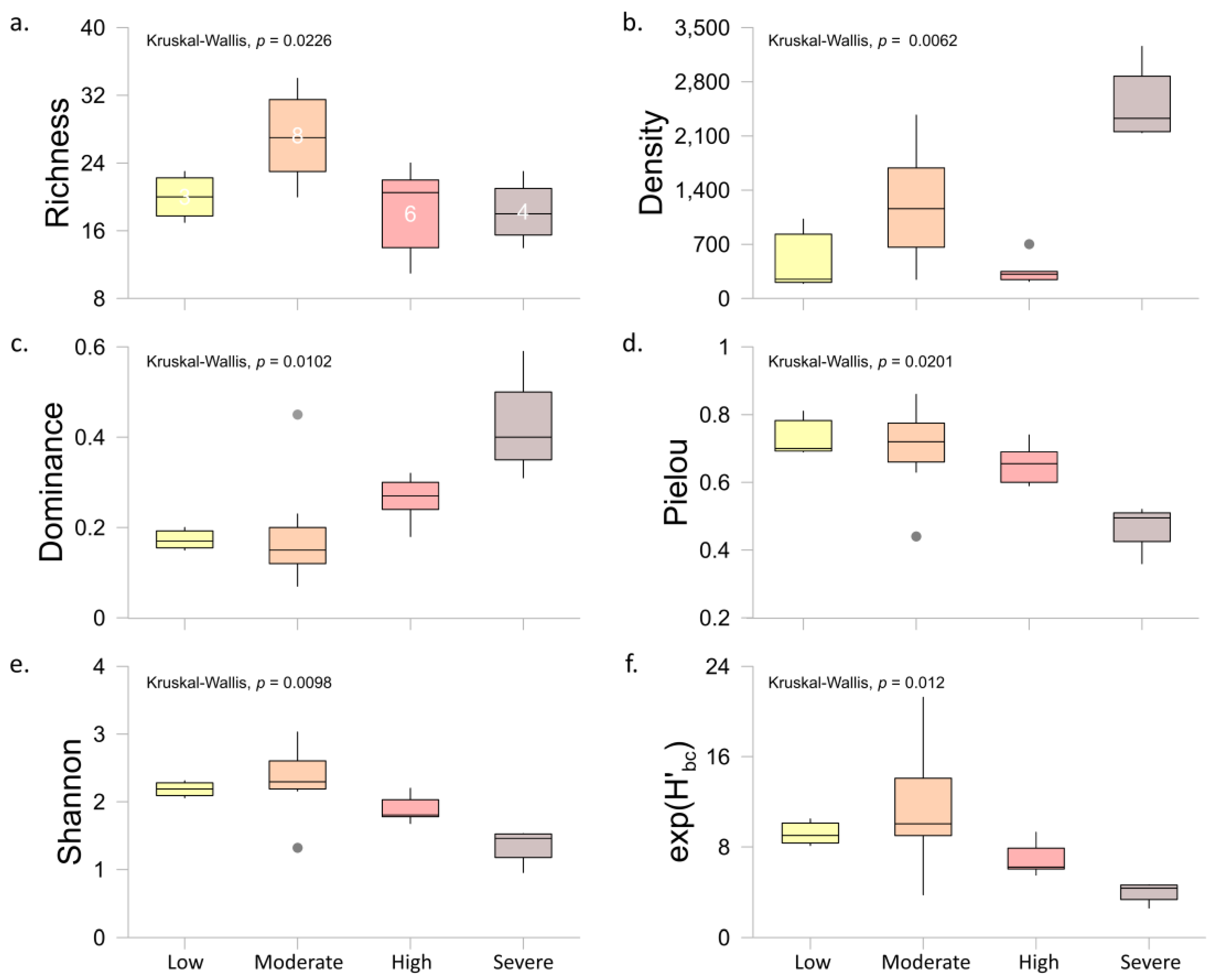
Besides the species composition, the ecological descriptors show the highest density values (up to 3758 ind./50 cc) under severe organic pollution conditions, where the highest dominance (up to 0.71) and lowest equitability (from 0.27 to 0.64) values occur. On the other hand, richness and Shannon diversity show the highest values (up to 27 and 4.27, respectively) under moderate organic pollution conditions (Supplementary Materials S6, Figure 5).
Leave-one-out cross-validation (jackknife) was employed to validate the LDA model. The resulting confusion matrix is presented in Table 3. The overall accuracy of 70% suggests that the discriminant model performs reasonably well in assigning each sample to its expected group. Notably, the severe pollution group achieved the highest accuracy, correctly classifying 91.7% of samples. Conversely, the low pollution group exhibited the highest error rate, with 44.4% of samples misclassified. Notably, the low pollution group comprised only three sites, totaling nine samples.

3.3.3. Indicator Value Index (IndVal)

The IndVal analysis identified six foraminiferal species as the major indicator species (IndVal > 35%; p < 0.05), reflecting varying levels of organic pollution across the study area (Table 4). These species include Ammonia tepida, Ammonia sp.1, Bulimina elongata, Cribroelphidium poeyanum, Paratrochammina sp.1, and Triloculina sp.1. Ammonia tepida exhibited the highest IndVal (64.16%; p = 0.001) and was associated with less impacted sites. Triloculina sp.1 and B. elongata were identified as moderately organic-polluted zone indicators. High pollution status was correlated with Paratrochammina sp.1 and Cribroelphidium poeyanum, while severely impacted sites were characterized by Ammonia sp.1 as the organic pollution indicator species (Table 4).

3.3.4. EcoQs vs. Organic Pollution Level

Fisher’s exact test revealed a significant association between EcoQS and the level of organic pollution (p < 0.05). The result of Goodman–Kruskal’s gamma, a non-parametric measure of the strength and direction of the association, revealed a strong negative association between these two ordinal variables (γ = −0.72), indicating that as EcoQS decreases (from “Excellent” to “Poor”), OrgPoll increases (from “Low” to “Severe”). A contingency table comparing the classifications of the EcoQS and OrgPoll is provided in Table 5.
The most frequent ecological quality status was “Bad” and “Moderate”, accounting for 87% of the observations. The strongest agreements occurred in the “Moderate-Moderate” category (22.2%) and the “Severe-Bad” category (20.6%). Notably, the “Bad” category for EcoQS appeared across all organic pollution levels.
The ordinal logistic regression model, with OrgPoll as a predictor of EcoQS, showed a statistically significant improvement in fit over the null model (Likelihood-ratio Test χ2 = 35.18, p < 0.001). The model yielded a McFadden’s Pseudo-R2 of 0.25. The regression coefficient for OrgPoll was negative and highly significant (β = −3.08, p < 0.001), with an estimated odds ratio of 0.046 (95% CI: 0.009–0.246). This means that a one-level increase in organic pollution reduces the odds of achieving better ecological quality status by approximately 95%, with the actual effect likely lying between 75% and 99%.
EcoQS variable was categorized into two classes: success (including “Good”, “Excellent”, and “Moderate”) and failure (“Poor” and “Bad”). The proportion of sites with EcoQS ≥ Moderate across the organic pollution categories is shown in Figure 6. The Cochran-Armitage trend test indicated a highly significant monotonic trend (Z = −4.71, p < 0.01). The chance of achieving at least Moderate EcoQS increased substantially as pollution decreased, rising from less than 10% under Severe pollution to over 75% under Low pollution.

4. Discussion

4.1. Environmental Characterization

The Santos Estuarine System’s hydrodynamics, as shown in Seiler et al. [51] and Reid et al. [89], presents varying energy conditions. The main channels, especially the Santos channel, show high-energy conditions. These channels are well flushed, with the Santos channel presenting net water import conditions and the São Vicente and Bertioga channels presenting net water export [51]. The Santos channel starkly contrasts with the low-energy, poorly flushed areas, such as the upper estuary, the broad middle section of the Bertioga Channel, and specific zones in the São Vicente Channel. This hydrodynamic partitioning directly dictates the sediment grain size and the distribution of carbonate content. The observed accumulation of fine-grained sediments in low-energy areas is expected due to reduced tidal currents, which allow the deposition of silt and clay particles and also induce organic pollution across the whole area (Table 2, Figure 2 and Figure 3).
The sediment type is often associated with higher organic matter content and greater potential for adsorbing pollutants. Thus, the distribution of benthic foraminifera is not a random phenomenon but a direct response to the physical and chemical gradients defined by the system’s hydrodynamics. The findings of Seiler et al. [51] and Reid et al. [89], based on observations and three-dimensional numerical modeling experiments, provide the essential framework for deciphering this relationship and help explain the observed foraminiferal patterns and their responses to organic pollutants.
Circulation patterns control key habitat variables for benthic organisms, including substrate type, oxygen availability, stratification, and salinity distribution (e.g., [90]). Seiler et al. [51] demonstrated a system of distinct hydrodynamic sub-environments. Consequently, these areas are predicted to host assemblages dominated by opportunistic and pollution-tolerant species, which thrive in organically enriched. The significant correlation obtained between the relative abundance of benthic foraminifera species and δ salinity values confirms the influence of the hydrodynamic on the microfauna in the Santos Estuarine System, occurring Paratrochammina sp.1 and species of Cribroelphidium in areas of higher δ salinity, and species of Bolivina, Bulimina and Nonionella in regions of marine influence.

4.2. System Quality Assessment Using Foraminifera

The K-means analysis shows an environmental quality gradient in the study area, with severe organic pollution mainly in the upper estuary, increasing in ecological quality towards the São Vicente and Bertioga channels, where high and moderate status prevail, and achieving low status in the lower estuary. The ecological descriptors follow this environmental quality gradient, showing high dominance and low equitability in the upper estuary, although density values are higher in this sector. This may be explained by the predominance of Ammonia sp. 1, which should be considered a tolerant species to severe organic pollution. In contrast, the channels and the low estuary have higher richness and Shannon diversity values.
In addition, as defined by discriminant analysis and complemented by the Indicator Value (IndVal) analysis, the opportunistic and pollution-tolerant foraminiferal species (A. parkinsoniana, Ammonia tepida, Ammonia sp.1, Bulimina elongata, C. poeyanum, Cribroelphidium spp., Paratrochammina sp.1, Paratrochammina spp., Triloculina sp.1) indicate ecological compartments in the Santos Estuarine System, and can be used as bioindicators of environmental quality in a region impacted by organic pollutants.
Ammonia tepida is the indicator species of low organic pollution conditions in the area. Ammonia tepida is an opportunistic species predominant in sediments of transitional environments worldwide (e.g., [91,92]), especially in bays, lagoons, and estuaries with higher organic matter content. This species has a high tolerance to environmental variations [93], being able to live in environments with high environmental stress, as well as higher levels of trace metals, fertilizers, and hydrocarbons [20,94,95]. However, our results show this species in samples with low organic pollution, associated mainly with coprostanol, suggesting that hydrocarbons are a stressor for this species. Coprostanol (5β-cholestan-3β-ol) is commonly used to indicate fecal contamination because it accounts for approximately 60% of the sterol composition in human feces [96,97,98]. The occurrence of this species in stations with low and high salinity variation values confirms its tolerance to salinity variations [20,90], and many other environmental parameters [93] may explain why this species does not exhibit an evident ecological response to some abiotic parameters, as occurs in the study area. Nonetheless, the low number of stations where A. tepida is considered the indicator species, but it does not allow us to draw assertive conclusions.
On the other hand, Ammonia sp.1 was observed in environments of severe environmental stress, apparently occupying the niche of A. tepida, being dominant in the upper estuary region, which has a very fine particle size, presenting the worst environmental conditions in the study area, with severe organic pollution (PAHs and coprostanol) [20], in addition to intermediate TOC values and low stratified estuary, according to salinity variations. In these severe organic pollution conditions, specimens of Ammonia sp. 1, together with individuals of A. tepida and A. parkinsoniana, exhibit abnormalities, such as aberrantly shaped chambers, reduced size, overdeveloped chambers, compressed tests, chambers growing along various axes of the tests, and tests with an excessively high spiral side, according to Polovodova and Schönfeld [99] classification.
Specimens of the genus Paratrochammina spp. have been recorded along the Brazilian coast, associated with mangroves [100,101,102]. In the present study, Paratrochammina sp.1 is associated in the Bertioga channel with C. poeyanum, classified as highly organically polluted in a stratified estuary, characterized by high salinity variations. The significant positive correlation between their abundance and the δ salinity values confirms these species as indicators of these environmental conditions.
Cribroelphidium spp. has been classified as an organic enrichment stress-tolerant and opportunistic taxon ([103] as Elphidium spp.). The Bertioga channel is characterized by very fine granulometry, rich in organic matter (UCM/ResAhs and LABs) and TOC, and with low marine influence and high salinity variation. The UCM/ResAhs suggested recent pollution introduction of oil that has been diluted by natural inputs [81,82,83], while LABs suggest a contamination by surfactants and detergents containing linear alkylbenzene sulphonates, probably from sewage input [104,105].
In the lower estuary and São Vicente stations, Bulimina elongata and Triloculina sp.1 were observed, with moderate levels of organic pollution, significant marine influence, and greater influence of AHs (petroleum input—[79,80]) and TOC. The significant negative correlation of relative abundance of B. elongata with the δ salinity values confirms its preference for marine conditions. Bulimina elongata has been characterized as a species tolerant of diverse environmental conditions, occurring in areas with high levels of hydrocarbons and TOC [106,107]. Although the miliolids are characteristic of environments rich in sandy sediments [106], Triloculina sp.1 was observed in some regions with high mud content (S5, S7, S8) and susceptible to increased organic matter.

4.3. Predictors of Organic Polluted Zones and EcoQs

The predicted class distribution generally shows a high percentage of correctly predicted samples for each organic pollution group, with the severe pollution group achieving the highest accuracy, showing that the presence and relative abundance of opportunistic and tolerant benthic foraminifera species can be used as predictors of the ecological environmental quality in the Santos Estuarine System. Still, the low-pollution group exhibited the highest error rate, indicating that samples can be misclassified. The replicate samples from two of these sites (SV1 and SV2) in the São Vicente Estuary were misclassified as moderate pollution (n = 3) and high pollution (n = 1). The species community in these sites is neither controlled by organic enrichment nor by natural stressors, such as sediment granulometry and salinity, which leads us to conclude that the misclassification may be due to the low number of samples analyzed.
Concerning EcoQS and organic pollution level, the most frequent ecological quality status was “Bad” and “Moderate”. Strongest agreements occurred in the “Moderate-Moderate” and “Severe-Bad” cells. Although the “Bad” category for EcoQS appeared across all organic pollution levels, the highest percentage of samples is classified as high or severe organic pollution.
Moreover, the model yielded a McFadden’s Pseudo-R2 of 0.25, which is considered a good fit in ecological applications, indicating that organic pollution explained a substantial portion of the variability in ecological quality status. The Cochran-Armitage trend test revealed a highly significant monotonic trend with the negative sign confirming that higher pollution scores corresponded to lower EcoQS outcomes.
These results demonstrate that integrating foraminiferal assemblages with organic chemistry data provides a sensitive framework for assessing the ecological quality of an estuarine system. The consistency between EcoQS classification and organic pollution levels can be effectively used as complementary tools to biomonitoring. The application of this methodology can support environmental agencies (e.g., CETESB), in defining thresholds for ecological quality, guiding mitigation strategies, and improving the management of a highly urbanized and industrialized coastal system such as the Santos Estuarine System.

5. Conclusions

Hydrodynamics in the Santos Estuarine System dictate the distribution of environmental parameters, favoring the deposition of fine sediments in the Upper Estuary, the Bertioga Channel, and most São Vicente Channel stations. This granulometric pattern, in turn, establishes the occurrence of organic pollutants in the system. Moreover, circulation patterns in the system control stratification and salinity variations, thereby establishing distinct sub-environments that host different benthic foraminiferal assemblages. The results delineate four distinct stages of organic pollution: low (observed in the Lower estuary–São Vicente channel and Santos Bay), moderate (in the Santos Channel), high (in the Bertioga Channel), and severe (in the Upper Estuary). Overall, the foraminiferal assemblages comprise opportunistic and pollution-tolerant species, which can be used as predictors of the environmental quality conditions in the estuarine system, as well as the ecological descriptors. Our analytical database indicates that the overall accuracy of 70% suggests the discriminant model performs reasonably well at assigning each sample to its expected organic pollution group. Our results show strong agreement between the EcoQS status classification and organic pollution levels confirming the effectiveness of this index based on benthic foraminifera in evaluating the state of health of the highly urbanized and impacted Santos Estuarine System.

Supplementary Materials

The following supporting information can be downloaded at: https://www.mdpi.com/article/10.3390/w18020172/s1, S1—Sampling dates, coordinates (Datum SIRGAS 2000), location, water depths, and vessels used. S2—Percentages and Concentrations distribution of (a) silt + clay, (b) total organic carbon (TOC), (c) calcium carbonate, (d) polycyclic aromatic hydrocarbons (PAHs), (e) aliphatic hydrocarbons (AHs), (f) linear alkylbenzenes (LABs), (g) unresolved complex mixture/resolved aliphatics ratio (UCM/ResAHs) in the study area. (h) coprostanol, and (i) Δ salinity values in the study area. S3—Box-plot graphs of Concentrations of (a) total organic carbon (TOC), (b) aliphatic hydrocarbons (AHs), (c) polycyclic aromatic hydrocarbons (PAHs), (d) linear alkylbenzenes (LABs), (e) coprostanol, and (f) unresolved complex mixture/resolved aliphatics ratio (UCM/ResAHs) in the study area. S4—Density (individuals per 50 cm3) of benthic foraminiferal taxa identified in surface sediment samples from the Bertioga Channel and São Vicente Channel in the Santos Estuarine System. S5—Density (individuals per 50 cm3) of benthic foraminiferal taxa identified in surface sediment samples from the Santos Upper Estuary, Channel and Bay in the Santos Estuarine System. S6—Richness (S), density of living specimens (number of individuals/50 cm3), Dominance index, Shannon-Wiener Diversity (H’), Pielou’s Equitability index, and Ecological Quality Status (EcoQS) in the study area.

Author Contributions

Conceptualization, S.H.d.M.e.S. and B.V.D.; Methodology, S.H.d.M.e.S., B.V.D., C.B., F.R.d.S., E.S., C.Y., J.S., B.S. and M.V.A.M.; Validation, E.S.; Formal analysis, S.H.d.M.e.S., B.V.D., C.B., F.R.d.S., E.S., C.Y., J.S., B.S., M.V.A.M., M.C.B. and R.C.L.F.; Investigation, S.H.d.M.e.S., B.V.D., C.B., E.S., C.Y., J.S. and B.S.; Resources, S.H.d.M.e.S., E.S., M.C.B. and R.C.L.F.; Data curation S.H.d.M.e.S., B.V.D., F.R.d.S., E.S., C.Y., J.S. and B.S.; Writing—original draft, S.H.d.M.e.S., B.V.D., C.B., F.R.d.S., E.S., C.Y., J.S., B.S. and M.V.A.M.; Writing—review & editing, S.H.d.M.e.S., B.V.D., C.B., F.R.d.S., E.S., C.Y., J.S., B.S., M.V.A.M., M.C.B. and R.C.L.F.; Visualization, S.H.d.M.e.S., B.V.D., C.B., F.R.d.S., E.S., C.Y., J.S., B.S., M.V.A.M., M.C.B. and R.C.L.F.; Supervision, S.H.d.M.e.S., C.B., E.S., R.C.L.F. and M.C.B.; Project administration, S.H.d.M.e.S., R.C.L.F. and M.C.B.; Funding acquisition, S.H.d.M.e.S., R.C.L.F. and M.C.B. All authors have read and agreed to the published version of the manuscript.

Funding

This work received support from the São Paulo Research Foundation (FAPESP, Projects 2019/13833-7, 2024/04114-5). J.S. acknowledges support from the São Paulo Research Foundation (Grant 2025/02658-0). SHMS, CB, ES, MCB, RCLF are Brazilian National Council for Scientific and Technological (CNPq) research fellows. C.Y. is fellow CNPq (385458/2025-8).

Data Availability Statement

The original contributions presented in this study are included in the article/Supplementary Material. Further inquiries can be directed to the corresponding author.

Acknowledgments

The authors would like to thank the editor and the anonymous reviewers for their constructive comments and suggestions, which significantly improved the quality of this manuscript. Financial support from FAPESP and CNPq is gratefully acknowledged. The authors also thank all collaborators involved in field sampling and the teams of the Laboratório de Dinâmica Costeira, Laboratório de Química Orgânica, Laboratório de Química Inorgânica, and Laboratório de Bioindicadores Ambientais at the Oceanographic Institute for their support during sample processing and analyses.

Conflicts of Interest

The authors declare no conflicts of interest.

Abbreviations

The following abbreviations are used in this manuscript:
EcoQSEcological Quality Status Index
AHsAliphatic
PAHsPolycyclic Aromatic Hydrocarbons
LABsLinear alkylbenzenes
LDALinear Discriminant Analysis
POPsPersistent Organic Pollutants
SDGSustainable Development in its Sustainable Development Goal
IPEAInstitute for Applied Economic Research
CETESBEnvironmental Company of the State of São Paulo
TOCTotal Organic Carbon
GCGas Chromatograph
FIDFlame Ionization Detector
BSTFABis (Trimethylsilyl) Trifluoroacetamide
TMCSTrimethylchlorosilane
UCM/ResAHsUnresolved Complex Mixture/Resolved Aliphatics ratio
A. tepidaAmmonia tepida
B. striatulaBolivina striatula
B. elongataBulimina elongata
C. excavatumCribroelphidium excavatum
C. poeyanumCribroelphidium poeyanum
IndValIndicator Value

References

  1. Cosby, A.G.; Lebakula, V.; Smith, C.N.; Wanik, D.W.; Bergene, K.; Rose, A.N.; Swanson, D.; Bloom, D.E. Accelerating Growth of Human Coastal Populations at the Global and Continent Levels: 2000–2018. Sci. Rep. 2024, 14, 22489. [Google Scholar] [CrossRef] [PubMed]
  2. Adger, W.N.; Hughes, T.P.; Folke, C.; Carpenter, S.R.; Rockström, J. Social-Ecological Resilience to Coastal Disasters. Science 2005, 309, 1036–1039. [Google Scholar] [CrossRef] [PubMed]
  3. Newton, A.; Carruthers, T.J.B.; Icely, J. The Coastal Syndromes and Hotspots on the Coast. Estuar. Coast. Shelf Sci. 2012, 96, 39–47. [Google Scholar] [CrossRef]
  4. Li, H. Management of Coastal Mega-Cities—A New Challenge in the 21st Century. Mar. Policy 2003, 27, 333–337. [Google Scholar] [CrossRef]
  5. Crain, C.M.; Halpern, B.S.; Beck, M.W.; Kappel, C.V. Understanding and Managing Human Threats to the Coastal Marine Environment. Ann. N. Y. Acad. Sci. 2009, 1162, 39–62. [Google Scholar] [CrossRef]
  6. Bulleri, F.; Chapman, M.G. The Introduction of Coastal Infrastructure as a Driver of Change in Marine Environments. J. Appl. Ecol. 2010, 47, 26–35. [Google Scholar] [CrossRef]
  7. Sekovski, I.; Newton, A.; Dennison, W.C. Megacities in the Coastal Zone: Using a Driver-Pressure-State-Impact-Response Framework to Address Complex Environmental Problems. Estuar. Coast. Shelf Sci. 2012, 96, 48–59. [Google Scholar] [CrossRef]
  8. Emnet, P.; Gaw, S.; Northcott, G.; Storey, B.; Graham, L. Personal Care Products and Steroid Hormones in the Antarctic Coastal Environment Associated with Two Antarctic Research Stations, McMurdo Station and Scott Base. Environ. Res. 2015, 136, 331–342. [Google Scholar] [CrossRef]
  9. Pereira, C.D.S.; Maranho, L.A.; Cortez, F.S.; Pusceddu, F.H.; Santos, A.R.; Ribeiro, D.A.; Cesar, A.; Guimarães, L.L. Occurrence of Pharmaceuticals and Cocaine in a Brazilian Coastal Zone. Sci. Total Environ. 2016, 548–549, 148–154. [Google Scholar] [CrossRef]
  10. Cantwell, M.G.; Katz, D.R.; Sullivan, J.C.; Lyman, M. Evaluation of Wastewater Tracers to Predict Pharmaceutical Distributions and Behavior in the Long Island Sound Estuary. Chemosphere 2019, 220, 629–636. [Google Scholar] [CrossRef]
  11. Fontes, M.K.; de Campos, B.G.; Cortez, F.S.; Pusceddu, F.H.; Moreno, B.B.; Maranho, L.A.; Lebre, D.T.; Guimarães, L.L.; Pereira, C.D.S. Seasonal Monitoring of Cocaine and Benzoylecgonine in a Subtropical Coastal Zone (Santos Bay, Brazil). Mar. Pollut. Bull. 2019, 149, 110545. [Google Scholar] [CrossRef] [PubMed]
  12. Abreu, F.E.L.; Lima da Silva, J.N.; Castro, Í.B.; Fillmann, G. Are Antifouling Residues a Matter of Concern in the Largest South American Port? J. Hazard. Mater. 2020, 398, 122937. [Google Scholar] [CrossRef] [PubMed]
  13. Pusceddu, F.H.; Sugauara, L.E.; de Marchi, M.R.; Choueri, R.B.; Castro, Í.B. Estrogen Levels in Surface Sediments from a Multi-Impacted Brazilian Estuarine System. Mar. Pollut. Bull. 2019, 142, 576–580. [Google Scholar] [CrossRef] [PubMed]
  14. Peng, Q.; Song, J.; Li, X.; Yuan, H.; Liu, M.; Duan, L.; Zuo, J. Pharmaceutically Active Compounds (PhACs) in Surface Sediments of the Jiaozhou Bay, North China. Environ. Pollut. 2020, 266, 115245. [Google Scholar] [CrossRef]
  15. Yang, L.; Zhou, Y.; Shi, B.; Meng, J.; He, B.; Yang, H.; Yoon, S.J.; Kim, T.; Kwon, B.-O.; Khim, J.S.; et al. Anthropogenic Impacts on the Contamination of Pharmaceuticals and Personal Care Products (PPCPs) in the Coastal Environments of the Yellow and Bohai Seas. Environ. Int. 2020, 135, 105306. [Google Scholar] [CrossRef]
  16. IBGE Panorama Estado de São Paulo. Available online: https://cidades.ibge.gov.br/brasil/sp/panorama (accessed on 3 December 2024).
  17. Lamparelli, M.C. Sistema Estuarino de Santos e São Vicente; Companhia de Tecnologia de Saneamento Ambiental (CETESB): São Paulo, Brazil, 2001. [Google Scholar]
  18. Mourão, A.P.; Caragnani, C.; Caetano, S.F.; Corrêa, C.F. Relatório de Situação dos Recursos Hídricos da Baixada Santista. Available online: https://www.sigrh.sp.gov.br/public/uploads/documents//CBH-BS/17490/rs_2019_bs_atualizado_30_08_2019_final.pdf (accessed on 3 December 2024).
  19. Hortellani, M.A.; Sarkis, J.E.S.; Abessa, D.M.S.; Sousa, E.C.P.M. Avaliação da contaminação por elementos metálicos dos sedimentos do Estuário Santos—São Vicente. Quím. Nova 2008, 31, 10–19. [Google Scholar] [CrossRef]
  20. Damasio, B.V.; Timoszczuk, C.T.; Kim, B.S.M.; Sousa, S.H.d.M.e.; Bícego, M.C.; Siegle, E.; Figueira, R.C.L. Impacts of Hydrodynamics and Pollutants on Foraminiferal Fauna Distribution in the Santos Estuary (SE Brazil). J. Sediment. Environ. 2020, 5, 61–86. [Google Scholar] [CrossRef]
  21. Frontalini, F.; Coccioni, R. Benthic Foraminifera as Bioindicators of Pollution: A Review of Italian Research over the Last Three Decades. Rev. Micropaléontologie 2011, 54, 115–127. [Google Scholar] [CrossRef]
  22. Martins, M.V.A.; Rodrigues, R.; Pereira, E.; Miranda, P.; Laut, L.; Belart, P.; Villena, H.H.; Geraldes, M.C.; Sousa, S.H.d.M.e.; Duleba, W.; et al. Organic Pollution in the NE Sector of Guanabara Bay (SE, Brazil). J. Sediment. Environ. 2018, 3, 138–154. [Google Scholar] [CrossRef]
  23. Sousa, S.H.M.; Yamashita, C.; Semensatto, D.L.; Santarosa, A.C.A.; Iwai, F.S.; Omachi, C.Y.; Disaró, S.T.; Martins, M.V.A.; Barbosa, C.F.; Bonetti, C.H.C.; et al. Opportunities and Challenges in Incorporating Benthic Foraminifera in Marine and Coastal Environmental Biomonitoring of Soft Sediments: From Science to Regulation and Practice. J. Sediment. Environ. 2020, 5, 257–265. [Google Scholar] [CrossRef]
  24. Rostami, M.A.; Frontalini, F.; Giordano, P.; Francescangeli, F.; Alves Martins, M.V.; Dyer, L.; Spagnoli, F. Testing the Applicability of Random Forest Modeling to Examine Benthic Foraminiferal Responses to Multiple Environmental Parameters. Mar. Environ. Res. 2021, 172, 105502. [Google Scholar] [CrossRef] [PubMed]
  25. Sambugaro, J.; Kropiwiec, I.S.; Pereira, L.G.; Sarmiento, J.A.S.; Magalhães, R.H.; Siegle, E.; Lopes Figueira, R.C.; Alves Martins, M.V.; Bouchet, V.M.P.; Frontalini, F.; et al. Contrasting Natural and Anthropic Historical Changes in Two Estuarine Systems on the Brazilian Coast: Benthic Foraminiferal-Based Paleo-Ecological Quality Status. Mar. Environ. Res. 2025, 210, 107306. [Google Scholar] [CrossRef] [PubMed]
  26. Murray, J.W. Biodiversity of Living Benthic Foraminifera: How Many Species Are There? Mar. Micropaleontol. 2007, 64, 163–176. [Google Scholar] [CrossRef]
  27. Cesbron, F.; Geslin, E.; Jorissen, F.J.; Delgard, M.L.; Charrieau, L.; Deflandre, B.; Jézéquel, D.; Anschutz, P.; Metzger, E. Vertical Distribution and Respiration Rates of Benthic Foraminifera: Contribution to Aerobic Remineralization in Intertidal Mudflats Covered by Zostera Noltei Meadows. Estuar. Coast. Shelf Sci. 2016, 179, 23–38. [Google Scholar] [CrossRef]
  28. Schönfeld, J.; Alve, E.; Geslin, E.; Jorissen, F.; Korsun, S.; Spezzaferri, S. The FOBIMO (FOraminiferal BIo-MOnitoring) Initiative—Towards a Standardised Protocol for Soft-Bottom Benthic Foraminiferal Monitoring Studies. Mar. Micropaleontol. 2012, 94–95, 1–13. [Google Scholar] [CrossRef]
  29. Jayaraju, N.; Sundara Raja Reddy, B.C.; Reddy, K.R. Anthropogenic Impact on Andaman Coast Monitoring with Benthic Foraminifera, Andaman Sea, India. Environ. Earth Sci. 2011, 62, 821–829. [Google Scholar] [CrossRef]
  30. Vidović, J.; Dolenec, M.; Dolenec, T.; Karamarko, V.; Žvab Rožič, P. Benthic Foraminifera Assemblages as Elemental Pollution Bioindicator in Marine Sediments around Fish Farm (Vrgada Island, Central Adriatic, Croatia). Mar. Pollut. Bull. 2014, 83, 198–213. [Google Scholar] [CrossRef]
  31. Prazeres, M.; Pandolfi, J.M. Effects of Elevated Temperature on the Shell Density of the Large Benthic Foraminifera Amphistegina Lobifera. J. Eukaryot. Microbiol. 2016, 63, 786–793. [Google Scholar] [CrossRef]
  32. O’Brien, P.A.J.; Polovodova Asteman, I.; Bouchet, V.M.P. Benthic Foraminiferal Indices and Environmental Quality Assessment of Transitional Waters: A Review of Current Challenges and Future Research Perspectives. Water 2021, 13, 1898. [Google Scholar] [CrossRef]
  33. Bouchet, V.M.P.; Alve, E.; Rygg, B.; Telford, R.J. Benthic Foraminifera Provide a Promising Tool for Ecological Quality Assessment of Marine Waters. Ecol. Indic. 2012, 23, 66–75, Erratum in Ecol. Indic. 2013, 26, 183. https://doi.org/10.1016/j.ecolind.2012.10.002.. [Google Scholar] [CrossRef]
  34. Bouchet, V.M.P.; Goberville, E.; Frontalini, F. Benthic Foraminifera to Assess Ecological Quality Statuses in Italian Transitional Waters. Ecol. Indic. 2018, 84, 130–139. [Google Scholar] [CrossRef]
  35. Bouchet, V.M.P.; Deldicq, N.; Baux, N.; Dauvin, J.-C.; Pezy, J.-P.; Seuront, L.; Méar, Y. Benthic Foraminifera to Assess Ecological Quality Statuses: The Case of Salmon Fish Farming. Ecol. Indic. 2020, 117, 106607. [Google Scholar] [CrossRef]
  36. Jesus, M.S.d.S.d.; Frontalini, F.; Bouchet, V.M.P.; Yamashita, C.; Sartoretto, J.R.; Figueira, R.C.; Sousa, S.H.d.M.e. Reconstruction of the Palaeo-Ecological Quality Status in an Impacted Estuary Using Benthic Foraminifera: The Santos Estuary (São Paulo State, SE Brazil). Mar. Environ. Res. 2020, 162, 105121. [Google Scholar] [CrossRef] [PubMed]
  37. El Kateb, A.; Stalder, C.; Martínez-Colón, M.; Mateu-Vicens, G.; Francescangeli, F.; Coletti, G.; Stainbank, S.; Spezzaferri, S. Foraminiferal-Based Biotic Indices to Assess the Ecological Quality Status of the Gulf of Gabes (Tunisia): Present Limitations and Future Perspectives. Ecol. Indic. 2020, 111, 105962. [Google Scholar] [CrossRef]
  38. Franzo, A.; Caffau, M.; Nasi, F.; Marrocchino, E.; Paletta, M.G.; Bazzaro, M.; Cibic, T. Benthic Foraminifera for the Ecological Status Assessment of Tourist Marinas. Ecol. Indic. 2023, 147, 110006. [Google Scholar] [CrossRef]
  39. O’Brien, P.; Barrenechea Angeles, I.; Cermakova, K.; Pawlowski, J.; Alve, E.; Nordberg, K.; Polovodova Asteman, I. Assessing Environmental Quality in a Historically Polluted Fjord: A Comparison of Benthic Foraminiferal eDNA and Morphospecies Approaches. J. Geophys. Res. Biogeosci. 2024, 129, e2023JG007781. [Google Scholar] [CrossRef]
  40. Punniyamoorthy, R.; Murugesan, P.; Sanchez, A.; Francescangeli, F.; Frontalini, F. Assessing the Ecological Quality Status in Tropical Indian Estuaries: Testing the Applicability of Benthic Foraminiferal Indices. Environ. Sci. Pollut. Res. 2024, 31, 51604–51618. [Google Scholar] [CrossRef]
  41. Suguio, K.; Vieira, E.M.; Barcelos, J.H. Ecological Interpretations of the Foraminifera from the Santos Estuary Zone, State of São Paulo, Brazil. Bol. Parana. Geociências 1975, 33, 41. [Google Scholar]
  42. Bonetti, C. Foraminíferos Como Bioindicadores Do Gradiente de Estresse Ecológico Em Ambientes Costeiros Poluídos. Estudo Aplicado Ao Sistema Estuarino de Santos-São Vicente (SP, Brasil). Ph.D. Thesis, University of São Paulo, São Paulo, Brazil, 2000. [Google Scholar]
  43. Debenay, J.-P.; Duleba, W.; Bonetti, C.; De Melo, E.; Souza, S.H.; Eichler, B.B. Pararotalia cananeiaensis n. sp.: Indicator of Marine Influence and Water Circulation in Brazilian Coastal and Paralic Environments. J. Foraminifer. Res. 2001, 31, 152–163. [Google Scholar] [CrossRef]
  44. Geslin, E.; Debenay, J.-P.; Duleba, W.; Bonetti, C. Morphological Abnormalities of Foraminiferal Tests in Brazilian Environments: Comparison between Polluted and Non-Polluted Areas. Mar. Micropaleontol. 2002, 45, 151–168. [Google Scholar] [CrossRef]
  45. Díaz, T.L.; Rodrigues, A.R.; Eichler, B.B. Distribution of Foraminifera in a Subtropical Brazilian Estuarine System. J. Foraminifer. Res. 2014, 44, 90–108. [Google Scholar] [CrossRef]
  46. Siqueira, G.W.; Braga, E.d.S.; Pereira, S.d.F.P.; da Silva, E. da Distribuição do mercúrio em sedimentos de fundo no Estuário de Santos SP/Brasil. Rem Rev. Esc. Minas 2005, 58, 309–316. [Google Scholar] [CrossRef]
  47. Sondotécnica Engenharia De Solos, S. Comportamento Hidráulico e Sedimentológico Do Estuário Santista; Portobrás/INPH: São Paulo, Brazil, 1977; Volume 2, 180p. [Google Scholar]
  48. Harari, J.; de Camargo, R. Numerical Simulation of the Tidal Propagation in the Coastal Region of Santos (Brazil, 24°S 46°W). Cont. Shelf Res. 2003, 23, 1597–1613. [Google Scholar] [CrossRef]
  49. Harari, J.; de Mesquita, A.; Marone, E.; França, C.A.S.; Camargo, R.d.; Pereira, J.E.R.; Adão, C.J.G.P.; Sá Júnios, I.L. Technical Report of the Project: Flow Measurements in the Bay of Santos|Request PDF; FUNDESPA: São Paulo, Brazil, 1990. [Google Scholar]
  50. Roversi, F.; Rosman, P.; Harari, J. Análise Das Trajetórias Das Águas Continentais Afluentes Ao Sistema Estuarino de Santos. Rev. Bras. Recur. Hídricos 2016, 21, 242–250. [Google Scholar] [CrossRef]
  51. Seiler, L.; Figueira, R.C.L.; Schettini, C.A.F.; Siegle, E. Three-Dimensional Hydrodynamic Modeling of the Santos-São Vicente-Bertioga Estuarine System, Brazil. Reg. Stud. Mar. Sci. 2020, 37, 101348. [Google Scholar] [CrossRef]
  52. Harari, J.; França, C.a.S.; Camargo, R.d. Climatology and hidrography of Santos estuary. In Perspectives on Ingrated Coastal Zone Management in South America; IST Press: Lisbon, Portugal, 2008. [Google Scholar]
  53. Miranda, L.B.d.; Castro, B.M.; Kjerfve, B. Princípios de Oceanografia Física de Estuários; EdUSP: São Paulo, Brazil, 2002; Volume 42, ISBN 978-85-314-0675-1. [Google Scholar]
  54. Speranzini, B. On Physical Oceanography of the Santos Estuary. Master’s Thesis, Delft University of Technology, Delft, The Netherlands, 2017. [Google Scholar]
  55. Santos, E.O. Características Climáticas. In AZEVEDO, A. A Baixada Santista: Aspectos Geográficos; Volume 1—As Bases Físicas; Editora da Universidade de São Paulo: São Paulo, Brazil, 1965; pp. 95–150. [Google Scholar]
  56. Fúlfaro, V.J.; Ponçano, W.L. Sedimentação Atual Estuário e Baía de Santos: Um Modelo Geológicoaplicado a Projetos de Expansão Da Zona Portuária. In Anais do Congresso Brasileiro de Geologia e Engenharia; ABEGE: Rio de Janeiro, Brazil, 1976. [Google Scholar]
  57. Buzas, M.A.; Hayek, L.-A.C.; Jett, J.A.; Reed, S.A. Pulsating Patches: History and Analyses of Spatial, Seasonal, and Yearly Distribution of Living Benthic Foraminifera; Smithsonian Institution Scholarly Press: Washington, DC, USA, 2019. [Google Scholar]
  58. Walton, W.R. Techniques for Recognition of Living Foraminifera. Contribution of Cushman. Found. Foraminifer. Res. 1952, 3, 56–60. [Google Scholar]
  59. Lutze, G.F.; Altenbach, A. Technik Und Signifikanz Der Lebendfärbung Benthischer Foraminiferen Mit Bengalrot. In Geologisches Jahrbuch. Reihe A, Allgemeine und regionale Geologie BR Deutschland und Nachbargebiete, Tektonik, Stratigraphie, Paläontologie; E. Schweizerbart’sche Verlagsbuchhandlung in Kommission: Stuttgart, Germany, 1991; pp. 251–265. [Google Scholar]
  60. Fatela, F.; Taborda, R. Confidence Limits of Species Proportions in Microfossil Assemblages. Mar. Micropaleontol. 2002, 45, 169–174. [Google Scholar] [CrossRef]
  61. Ellis, B.F.; Messina, A.R. Catalogue of Foraminifera; Micropaleontology Press: Flushing, NY, USA, 1940. [Google Scholar]
  62. Boltovskoy, E.; Giussani, G.; Watanabe, S.; Wright, R. Systematics and Distribution. In Atlas of Benthic Shelf Foraminifera of the Southwest Atlantic; Boltovskoy, E., Giussani, G., Watanabe, S., Wright, R., Eds.; Springer: Dordrecht, The Netherlands, 1980; pp. 12–56. ISBN 978-94-009-9188-0. [Google Scholar]
  63. Loeblich, A.R.; Tappan, H. Foraminiferal Genera and Their Classification; Springer: London, UK, 1988; ISBN 978-1-4899-5760-3. [Google Scholar]
  64. Disaró, S. Foraminíferos Em Ecossistemas de Manguezal e Marismas Salgadas. In Revisões Em Zoologia-I: Volume Comemorativo Dos 30 Anos Do Curso de Pós-Graduação Em Zoologia Da Universidade Federal Do Paraná; Secretaria do Meio Ambiente do Estado do Paraná: Curitiba, Brazil, 2006; pp. 67–85. ISBN 85-99592-08-4. [Google Scholar]
  65. Worms Editorial Board Worms—World Register of Marine Species. Available online: https://www.marinespecies.org/ (accessed on 5 December 2024).
  66. Suguio, K. Introdução à Sedimentologia; Editora E. Blücher: São Paulo, Brazil, 1973. [Google Scholar]
  67. Walkley, A.; Black, I.A. An Examination of the Degtjareff Method for Determining Soil Organic Matter, and A Proposed Modification of the Chromic Acid Titration Method. Soil Sci. 1934, 37, 29–38. [Google Scholar] [CrossRef]
  68. UNEP (United Nations Environment Programme). Determination of Petroleum Hydrocarbons in Sediments; UNESCO: Paris, France, 1992. [Google Scholar]
  69. Sasaki, S.T. Marcadores Orgânicos Moleculares Como Ferramentas No Monitoramento Ambiental: Avaliação Da Distribuição de Alquilbenzeno Lineares (LABs) Em Organismos e Sedimentos, Como Indicativo de Exposição Ao Esgoto Em Áreas Costeiras. Ph.D. Thesis, Universidade de São Paulo, São Paulo, Brazil, 2012. [Google Scholar] [CrossRef]
  70. Santos, F.R.; Neves, P.A.; Kim, B.S.M.; Taniguchi, S.; Lourenço, R.A.; Timoszczuk, C.T.; Sotão, B.M.T.; Montone, R.C.; Figueira, R.C.L.; Mahiques, M.M.; et al. Organic Contaminants and Trace Metals in the Western South Atlantic Upper Continental Margin: Anthropogenic Influence on Mud Depocenters. Mar. Pollut. Bull. 2020, 154, 111087. [Google Scholar] [CrossRef]
  71. RStudio Team. RStudio: Integrated Development Environment for R; RStudio, PBC: Boston, MA, USA, 2020. [Google Scholar]
  72. Hausser, J.; Strimmer, K. Entropy Inference and the James-Stein Estimator, with Application to Nonlinear Gene Association Networks. J. Mach. Learn. Res. 2009, 10, 1469–1484. [Google Scholar]
  73. Chao, A.; Shen, T.-J. Nonparametric Estimation of Shannon’s Index of Diversity When There Are Unseen Species in Sample. Environ. Ecol. Stat. 2003, 10, 429–443. [Google Scholar] [CrossRef]
  74. Lê, S.; Josse, J.; Husson, F. FactoMineR: An R Package for Multivariate Analysis. J. Stat. Softw. 2008, 25, 1–18. [Google Scholar] [CrossRef]
  75. Venables, W.N.; Ripley, B.D. Modern Applied Statistics with S.; Statistics and Computing; Springer: New York, NY, USA, 2002; ISBN 978-1-4419-3008-8. [Google Scholar]
  76. Wickham, H. Ggplot2; Use R! Springer International Publishing: Cham, Germany, 2016; ISBN 978-3-319-24275-0. [Google Scholar]
  77. Dufrêne, M.; Legendre, P. Species Assemblages and Indicator Species: The Need for a Flexible Asymmetrical Approach. Ecol. Monogr. 1997, 67, 345–366. [Google Scholar] [CrossRef]
  78. Roberts, D.W. Labdsv: Ordination and Multivariate Analysis for Ecology. 2025. Available online: https://cran.r-project.org/web/packages/labdsv/labdsv.pdf (accessed on 3 December 2025).
  79. Volkman, J.K.; Holdsworth, D.G.; Neill, G.P.; Bavor, H.J. Identification of Natural, Anthropogenic and Petroleum Hydrocarbons in Aquatic Sediments. Sci. Total Environ. 1992, 112, 203–219. [Google Scholar] [CrossRef]
  80. Readman, J.W.; Fillmann, G.; Tolosa, I.; Bartocci, J.; Villeneuve, J.-P.; Catinni, C.; Mee, L.D. Petroleum and PAH Contamination of the Black Sea. Mar. Pollut. Bull. 2002, 44, 48–62. [Google Scholar] [CrossRef]
  81. Simoneit, B.R.T.; Lonsdale, P.F. Hydrothermal Petroleum in Mineralized Mounds at the Seabed of Guaymas Basin. Nature 1982, 295, 198–202. [Google Scholar] [CrossRef]
  82. Tolosa, I.; de Mora, S.; Sheikholeslami, M.R.; Villeneuve, J.-P.; Bartocci, J.; Cattini, C. Aliphatic and Aromatic Hydrocarbons in Coastal Caspian Sea Sediments. Mar. Pollut. Bull. 2004, 48, 44–60. [Google Scholar] [CrossRef]
  83. Gao, Y.; Han, Y.; Xia, J.; Tan, J.; Wang, Y.-P.; Wang, S. Composition and Distribution of Aliphatic Hydrocarbon Compounds and Biomarkers in Seafloor Sediments from Offshore of the Leizhou Peninsula (South China). ACS Omega 2021, 6, 34286–34293. [Google Scholar] [CrossRef]
  84. Baumard, P.; Budzinski, H.; Michon, Q.; Garrigues, P.; Burgeot, T.; Bellocq, J. Origin and Bioavailability of PAHs in the Mediterranean Sea from Mussel and Sediment Records. Estuar. Coast. Shelf Sci. 1998, 47, 77–90. [Google Scholar] [CrossRef]
  85. Hatcher, P.G.; McGillivary, P.A. Sewage Contamination in the New York Bight. Coprostanol as an Indicator. Environ. Sci. Technol. 1979, 13, 1225–1229. [Google Scholar] [CrossRef]
  86. Grimalt, J.O.; Fernandez, P.; Bayona, J.M.; Albaiges, J. Assessment of Fecal Sterols and Ketones as Indicators of Urban Sewage Inputs to Coastal Waters. Environ. Sci. Technol. 1990, 24, 357–363. [Google Scholar] [CrossRef]
  87. Writer, J.H.; Leenheer, J.A.; Barber, L.B.; Amy, G.L.; Chapra, S.C. Sewage Contamination in the Upper Mississippi River as Measured by the Fecal Sterol, Coprostanol. Water Res. 1995, 29, 1427–1436. [Google Scholar] [CrossRef]
  88. González-Oreja, J.A.; Saiz-Salinas, J.I. Short-Term Spatio-Temporal Changes in Urban Pollution by Means of Faecal Sterols Analysis. Mar. Pollut. Bull. 1998, 36, 868–875. [Google Scholar] [CrossRef]
  89. Reid, J.; Seiler, L.; Siegle, E. The Influence of Dredging on Estuarine Hydrodynamics: Historical Evolution of the Santos Estuarine System, Brazil. Estuar. Coast. Shelf Sci. 2022, 279, 108131. [Google Scholar] [CrossRef]
  90. Francescangeli, F.; Milker, Y.; Bunzel, D.; Thomas, H.; Norbisrath, M.; Schönfeld, J.; Schmiedl, G. Recent Benthic Foraminiferal Distribution in the Elbe Estuary (North Sea, Germany): A Response to Environmental Stressors. Estuar. Coast. Shelf Sci. 2021, 251, 107198. [Google Scholar] [CrossRef]
  91. Debenay, J.-P.; Guillou, J.-J. Ecological Transitions Indicated by Foraminiferal Assemblages in Paralic Environments. Estuaries 2002, 25, 1107–1120. [Google Scholar] [CrossRef]
  92. Bouchet, V.M.P.; Frontalini, F.; Francescangeli, F.; Sauriau, P.-G.; Geslin, E.; Martins, M.V.A.; Almogi-Labin, A.; Avnaim-Katav, S.; Di Bella, L.; Cearreta, A.; et al. Indicative Value of Benthic Foraminifera for Biomonitoring: Assignment to Ecological Groups of Sensitivity to Total Organic Carbon of Species from European Intertidal Areas and Transitional Waters. Mar. Pollut. Bull. 2021, 164, 112071. [Google Scholar] [CrossRef]
  93. Laut, L.L.M.; Clemente, I.M.M.M.; Belart, P.; Martins, M.V.A.; Frontalini, F.; Laut, V.M.; Gomes, A.; Boski, T.; Lorini, M.L.; Fortes, R.R.; et al. Multiproxies (Benthic Foraminifera, Ostracods and Biopolymers) Approach Applied to Identify the Environmental Partitioning of the Guadiana River Estuary (Iberian Peninsula). J. Sediment. Environ. 2016, 1, 178–195. [Google Scholar] [CrossRef]
  94. Armynot du Châtelet, E.; Debenay, J.-P.; Soulard, R. Foraminiferal Proxies for Pollution Monitoring in Moderately Polluted Harbors. Environ. Pollut. 2004, 127, 27–40. [Google Scholar] [CrossRef]
  95. Coccioni, R.; Frontalini, F.; Marsili, A.; Mana, D. Benthic Foraminifera and Trace Element Distribution: A Case-Study from the Heavily Polluted Lagoon of Venice (Italy). Mar. Pollut. Bull. 2009, 59, 257–267. [Google Scholar] [CrossRef]
  96. Leeming, R.; Ball, A.; Ashbolt, N.; Nichols, P. Using Faecal Sterols from Humans and Animals to Distinguish Faecal Pollution in Receiving Waters. Water Res. 1996, 30, 2893–2900. [Google Scholar] [CrossRef]
  97. Prost, K.; Birk, J.J.; Lehndorff, E.; Gerlach, R.; Amelung, W. Steroid Biomarkers Revisited—Improved Source Identification of Faecal Remains in Archaeological Soil Material. PLoS ONE 2017, 12, e0164882. [Google Scholar] [CrossRef]
  98. Santos, F.R.; Martins, D.A.; Morais, P.C.V.; Oliveira, A.H.B.; Gama, A.F.; Nascimento, R.F.; Choi-Lima, K.F.; Moreira, L.B.; Abessa, D.M.S.; Nelson, R.K.; et al. Influence of Anthropogenic Activities and Risk Assessment on Protected Mangrove Forest Using Traditional and Emerging Molecular Markers (Ceará Coast, Northeastern Brazil). Sci. Total Environ. 2019, 656, 877–888. [Google Scholar] [CrossRef]
  99. Polovodova, I.; Schönfeld, J. Foraminiferal Test Abnormalities in the Western Baltic Sea. J. Foraminifer. Res. 2008, 38, 318–336. [Google Scholar] [CrossRef]
  100. Laut, L.; da Matta, G.; Camara, G.; Belart, P.; Clemente, I.; Ballalai, J.; Volino, E.; Couto, E.d.C.G. Living and Dead Foraminifera Assemblages as Environmental Indicators in the Almada River Estuary, Ilhéus, Northeastern Brazil. J. S. Am. Earth Sci. 2021, 105, 102883. [Google Scholar] [CrossRef]
  101. Raposo, D.; Frontalini, F.; Clemente, I.; da Conceição Guerreiro Couto, E.; Veríssimo, F.; Laut, L. Benthic Foraminiferal Response to Trace Elements in a Tropical Mesotidal Brazilian Estuary. Estuaries Coasts 2022, 45, 2610–2631. [Google Scholar] [CrossRef]
  102. Fontana, L.F.; Belart, P.; Bonetti, C.; Junior, D.S.; Frontalini, F.; Martínez-Colón, M.; Bouchet, V.M.P.; Laut, L. Foraminifera and Geomicrobiology as Indicators of the Environmental Recovery in a Mangrove Affected by Oil Spills in the Guanabara Bay (Brazil). Sci. Total Environ. 2024, 957, 177650. [Google Scholar] [CrossRef]
  103. Alve, E. Benthic Foraminiferal Responses to Estuarine Pollution; a Review. J. Foraminifer. Res. 1995, 25, 190–203. [Google Scholar] [CrossRef]
  104. Zeng, E.Y.; Cheng, D.; Khan, A.R.; Vista, C.L. Validity of Using Linear Alkylbenzenes as Markers of Sewage Contamination with Interference from Tetrapropylene-based Alkylbenzenes. Environ. Toxicol. Chem. 1998, 17, 394–397. [Google Scholar] [CrossRef]
  105. Thomes, M.W.; Vaezzadeh, V.; Zakaria, M.P.; Bong, C.W. Use of Sterols and Linear Alkylbenzenes as Molecular Markers of Sewage Pollution in Southeast Asia. Environ. Sci. Pollut. Res. 2019, 26, 31555–31580. [Google Scholar] [CrossRef]
  106. Dimiza, M.D.; Ravani, A.; Kapsimalis, V.; Panagiotopoulos, I.P.; Skampa, E.; Triantaphyllou, M.V. Benthic Foraminiferal Assemblages in the Severely Polluted Coastal Environment of Drapetsona-Keratsini, Saronikos Gulf (Greece). Rev. Micropaléontologie 2019, 62, 33–44. [Google Scholar] [CrossRef]
  107. Eichler, P.P.B.; Eichler, B.B.; Vital, H. Marine Pollution-Environmental Indicators in Marine Meiofauna from Brazil. In Environmental Indicators; Armon, R.H., Hänninen, O., Eds.; Springer: Dordrecht, The Netherlands, 2015; pp. 545–560. ISBN 978-94-017-9499-2. [Google Scholar]
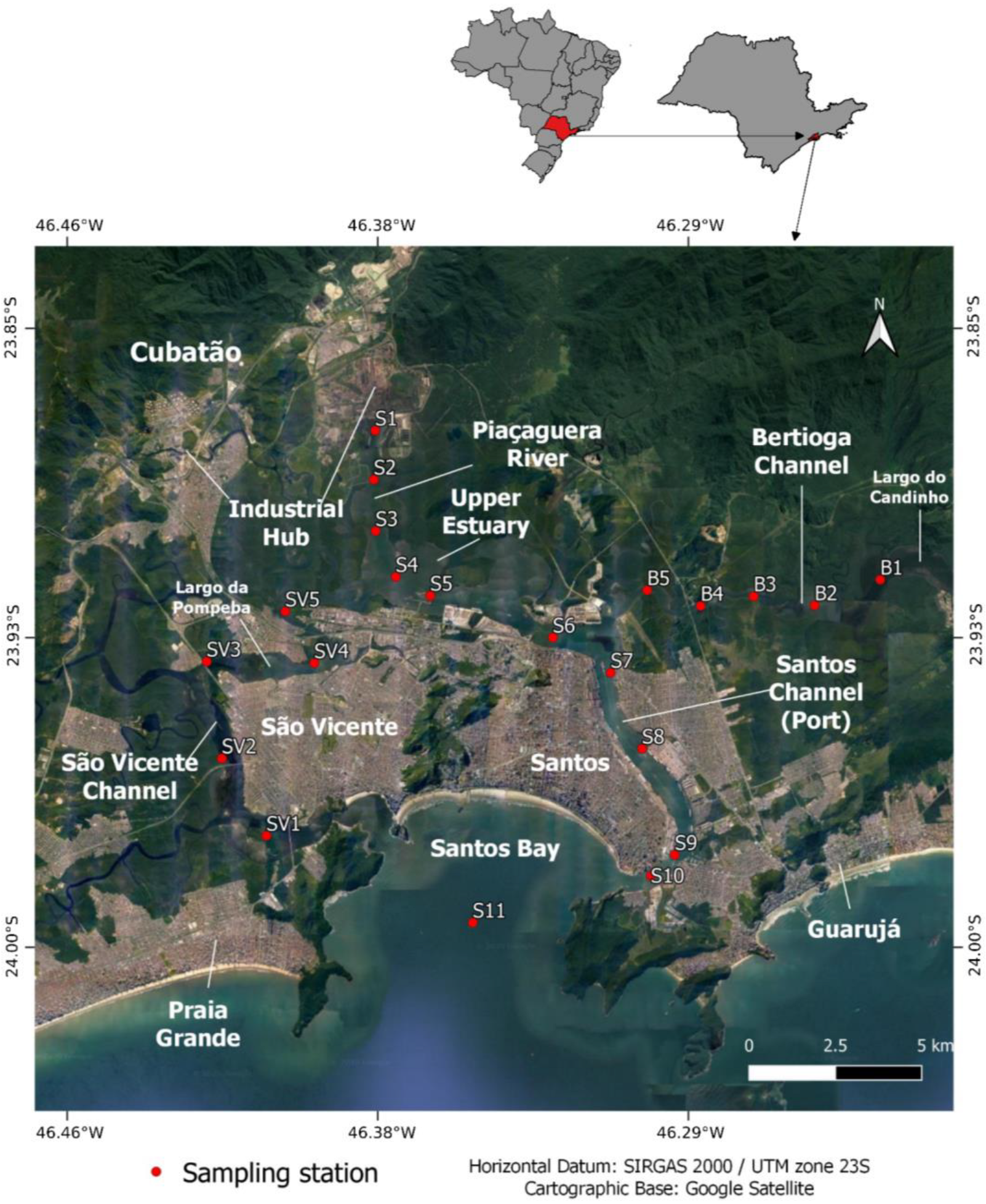
Figure 1. The study area: Estuarine System of Santos, São Vicente, and Bertioga, located on the south coast of the state of São Paulo, covers the municipalities of Praia Grande, São Vicente, Santos, Cubatão, Guarujá, and Bertioga. Red dots correspond to sampling stations on the São Vicente Channel (SV), the Santos Upper Estuary, Channel and Bay (S), and the Bertioga Channel (B).
Water 18 00172 g001
Figure 2. (a) Distribution and (b) Map of sampling sites across four clusters identified by K-means analysis. Sample labels consist of a regional code (SV = São Vicente Channel; S = Santos Upper Estuary, Channel and Bay; B = Bertioga Channel) and station number. Symbols and colors represent the organic pollution status (low, moderate, high, and severe).
Water 18 00172 g002
Figure 3. Boxplots of the variations in (a) total organic carbon (TOC, %), (b) linear alkylbenzenes (LABs), (c) aliphatic hydrocarbons (AHs, µg g−1), (d) polycyclic aromatic hydrocarbons (PAHs, ng g−1), (e) coprostanol (µg g−1), and (f) unresolved complex mixture/resolved aliphatics ratio (UCM/ResAHs) across sampling groups categorized by organic pollution status. The box represents the interquartile range (IQR), and horizontal lines across it correspond to the median values. The whiskers outside the box show minimum and maximum values excluding outliers, which are shown as individual dots. Numbers displayed inside the boxes in panel (a) indicate the number of samples (n) in each pollution category.
Water 18 00172 g003
Figure 4. Discriminant analysis ordination displaying the first and second discriminant functions (LD1 vs. LD2). Colored rings represent group centroids, matching the colors of the associated samples (filled circles). The vectors depict the coefficients of linear discriminants. Sample labels consist of a regional code (SV = São Vicente Channel; S = Santos Upper Estuary, Channel and Bay; B = Bertioga Channel), a station number, and a lowercase letter (a–c) indicating analytical replicates.
Water 18 00172 g004
Figure 5. Boxplots of the variations in (a) richness, (b) density (ind./50 cm3), (c) dominance, (d) Pielou’s Equitability index, (e) Shannon-Wiener Diversity (H’), and (f) exp(H’bc) across sampling groups categorized by organic pollution status. The box represents the interquartile range (IQR), and horizontal lines across it correspond to the median values. The whiskers outside the box show minimum and maximum values excluding outliers, which are shown as individual dots. Numbers displayed inside the boxes in panel (a) indicate the number of samples (n) in each pollution category.
Water 18 00172 g005
Figure 6. Proportion of samples with EcoQS ≥ Moderate (classified as “success”) across organic pollution categories. Points represent observed proportions of “success” cases, and error bars indicate 95% confidence intervals estimated using the Wilson method. The dashed line represents a fitted linear trend across the ordinal pollution score (Severe to Low), explaining 85% of the variation in success proportion across categories (R2 = 0.851).
Water 18 00172 g006
Table 1. Equation, threshold values, and classification of the Ecological Quality Status used in this study.
IndexAuthorsEquationThreshold ValuesEnvironmental Health Classification
Ecological Quality Status (EcoQS)Bouchet et al. [33,34]EcoQS = Exp(H’bc 1)>15Excellent
11–15Good
7–11Moderate
3–7Bad
<3Poor
1 H’bc: bias corrected Shannon’s index [73].
Table 2. Values in the total organic carbon (TOC), aliphatic hydrocarbons (AHs), polycyclic aromatic hydrocarbons (PAHs), linear alkylbenzenes (LABs), coprostanol, and unresolved complex mixture/resolved aliphatics ratio (UCM/ResAHs), percentage of mud, calcium carbonate (CaCO3), and salinity variation per station in the Santos Estuary System.
StationsTOCTotal Aliphatics Total PAHTotal LABsCoprostanolUCM/ResAHsMudCaCO3δ Salinity
%μg g−1ng g−1ng g−1μg g−1 %%
B14.7379.8522.2166.42.21.998.452.551.63
B25.47136.12354.6172.82.11.498.460.383.56
B34.87152.62769.8185.11.71.197.030.004.57
B45.37161.92851.7270.21.11.373.510.914.51
B50.8790.04437.092.60.62.117.260.553.63
S12.32317.518,102.262.20.66.688.970.001.16
S24.33321.712,955.287.34.66.489.063.451.56
S32.70250.76052.368.51.74.984.014.534.33
S42.60220.822,375.0104.84.54.595.390.001.83
S52.6996.11527.8179.40.56.689.028.411.68
S62.35152.53995.0937.91.65.890.746.781.51
S72.2064.61532.9210.51.12.382.1314.801.5
S82.2063.11378.795.90.43.080.994.551.11
S91.0529.31978.8231.90.12.024.3911.410.79
S101.2824.61468.0183.70.31.915.7713.220.64
S110.538.2214.7520.12.30.96.453.660.47
SV10.675.9104.585.70.50.414.848.583.51
SV22.699.1191.6266.41.40.645.301.562.33
SV32.3422.51335.1276.40.61.920.621.151.83
SV43.88112.11932.01382.84.73.491.772.782.38
SV50.67108.93186.9188.80.72.26.601.342.85
Table 3. Confusion matrix obtained by jackknife cross-validation showing the LDA predicted class labels on the rows and the expected (original) class labels on the columns. The diagonal cells show the percentage of correctly predicted samples for each organic pollution group.
Expected Class Distribution (%)
LowModerateHighSevere
Predicted Class Distribution (%)Low55.64.211.10
Moderate33.366.716.78.3
High11.116.761.10
Severe012.511.191.7
Number of Samples9241812
Table 4. Indicator Value index (IndVal) analysis identifying statistically significant indicator species for each organic pollution zone.
Organic Pollution StatusIndicator SpeciesIndVal (%)p-Value
LowAmmonia tepida64.160.001
ModerateTriloculina sp. 142.660.004
Bulimina elongata39.750.008
HighParatrochammina sp. 156.530.001
Cribroelphidium poeyanum40.040.015
SevereAmmonia sp.147.190.001
Table 5. Contingency table of Ecological Quality Status (EcoQS; “Poor” to “Excellent”) by organic-pollution level (OrgPoll; “Low” to “Severe”). Cell entries are percentages of all samples, and bold values are marginal totals.
PoorBadModerateGoodExcellentSum
Low03.1711.110014.29
Moderate06.3522.223.176.3538.09
High012.709.520022.22
Severe3.1720.631.590025.40
Sum3.1742.8644.443.26.3100
Disclaimer/Publisher’s Note: The statements, opinions and data contained in all publications are solely those of the individual author(s) and contributor(s) and not of MDPI and/or the editor(s). MDPI and/or the editor(s) disclaim responsibility for any injury to people or property resulting from any ideas, methods, instructions or products referred to in the content.