Article

Geospatial Assessment and Modeling of Water–Energy–Food Nexus Optimization for Sustainable Paddy Cultivation in the Dry Zone of Sri Lanka: A Case Study in the North Central Province

Division of Soil Resource and Water Environment, National Institute of Agricultural Sciences, Rural Development Administration, Iseo-myeon, Wanju-gun 55365, Jeollabuk-do, Republic of Korea
*
Author to whom correspondence should be addressed.
Water 2026, 18(2), 152; https://doi.org/10.3390/w18020152
Submission received: 13 November 2025 / Revised: 15 December 2025 / Accepted: 29 December 2025 / Published: 6 January 2026

Abstract

This study presents a geospatial assessment and modeling of the water–energy–food (WEF) nexus to enrich the sustainable paddy cultivation of the North Central Province (NCP) of Sri Lanka in the Dry Zone. Increasing climatic variability and limited resources have raised concerns about the need for efficient resource management to restore food security globally. The study analyzed the three components of the WEF nexus for their synergies and trade-offs using GIS and remote sensing applications. The food productivity potential was derived using the Normalized Difference Vegetation Index (NDVI), Soil Organic Carbon (SOC), soil type, and land use, whereas water availability was assessed using the Normalized Difference Water Index (NDWI), Soil Moisture Index (SMI), and rainfall data. Energy potential was mapped using WorldClim 2.1 datasets on solar radiation and wind speed and the proximity to the national grid. Scenario modeling was conducted through raster overlay analysis to identify zones of WEF constraints and synergies such as low food–low water areas and high energy–low productivity areas. To ensure the accuracy of the created model, Pearson correlation analysis was used to internally validate between hotspot layers (representing extracted data) and scenario layers (representing modeled outputs). The results revealed a strong positive correlation (r = 0.737), a moderate positive correlation for energy (r = 0.582), and a positive correlation for food (r = 0.273). Those values were statistically significant at p > 0.001. These results confirm the internal validity and accuracy of the model. This study further calculated the total greenhouse gas (GHG) emissions from paddy cultivation in NCP as 1,070,800 tCO2eq yr−1, which results in an emission intensity of 5.35 tCO2eq ha−1 yr−1, with CH4 contributing around 89% and N2O 11%. This highlights the importance of sustainable cultivation in mitigating agricultural emissions that contribute to climate change. Overall, this study demonstrates a robust framework for identifying areas of resource stress or potential synergy under the WEF nexus for policy implementation, to promote climate resilience and sustainable paddy cultivation, to enhance the food security of the country. This model can be adapted to implement similar research work in the future as well.

1. Introduction

Water, energy, and food are important resources that contribute to sustainable livelihoods and influence economic development. These three main resources are currently being subjected to overexploitation due to increased demand caused by the growing population, labor shortage, and expansion of the economy [1,2,3,4] (Cuthbert et al., 2022; Na et al., 2024; SADC, 2016; Yoon et al., 2022). Hence, an integrated approach that examines these three components is crucial for sustainable development [5] (Gonzalez, 2020). The concept of using a nexus to interpret the connections among water, energy, and food resources and to present an integrated management plan for these resources is called WEF nexus management [6] (Ringler et al., 2013). This concept helps to analyze the interconnections and trade-offs according to changes in each element by considering their interrelationships. Water, energy, and food systems interact in agriculture in multiple ways. Water and energy are required for food production; energy is required for water intake, water treatment, and distribution, fertilization, cultivation, harvesting, and transportation; water is used to produce energy; and food is used as fuel for energy [6,7] (Ringler et al., 2013; Daher et al., 2019). These interactions give rise to trade-offs or synergies; for example, more water allocated for irrigation leaves less water available for hydropower production [8] (Wu et al., 2021). This approach directly addresses three Sustainable Development Goals (SDGs)—zero hunger, clean water and sanitation, and affordable and clean energy—but indirectly impacts all 17 SDGs [5] (Gonzalez, 2020).
Sri Lanka’s NCP is a region predominantly reliant on paddy cultivation as the primary agricultural activity, performed mainly during the Yala (May to August) and Maha (September to March) cultivation periods, depending heavily on rainfall and irrigation [9] (Nandani and Vidanapathirana, 2024). With great variability of the climate, Sri Lanka has a diverse annual rainfall distribution. The country can be divided in to three climatic zones: the Dry Zone (DZ) with rainfall below 1750 mm, Intermediate Zone (IZ) with rainfall varying between 1750 mm and 2500 mm, and the Wet Zone (WZ) with rainfall above 2500 mm [10] (Salman et al., 2023). Rice is the staple food of the Sri Lankan diet, which has an annual per capita consumption of 100 kg, 40 kg more than the global average [11] (Gamawelagedara et al., 2011). Over 30% of agricultural land is cultivated with rice, the majority of which is located in the northern part of the DZ in the country [12] (Department of Census and Statistics, 2017). Paddy farming is a major socioeconomic activity, which directly employs 72% of the rural population. Due to ongoing land fragmentation, more than 50% of total rice production comes from smallholder farmers who cultivate less than 0.4 ha per household. Most smallholder farmers are settled in the DZ, where they practice irrigated rice farming, which plays an important role in poverty alleviation, local employment generation, and ensuring household food security [10] (Salman et al., 2023). Although the average rice production in the country amounts to 3.71 million tons a year, compared to other rice-producing countries, low yields and the low resource use efficiency in the region are still a challenge [10] (Salman et al., 2023).
Rice crop requires more water than any other crop that is being cultivated. Water plays a crucial role in plant physiology, and also it plays an important role in management practices such as nursery preparation, transplanting, weeding, fertilizer application, and pest and disease control [10] (Salman et al., 2023). Sri Lanka, where paddy rice is cultivated under a continuous flooding system, consumes around 2500 L of water to produce just 1 kg of rice, which places immense pressure on the water resources and supply, especially in drought periods [13] (DailyFT, 2024). The average water use of paddy cultivation in Sri Lanka is around twice that of other paddy-growing countries. The main reasons for this are the low water use efficiency, low water productivity due to a lack of on-farm management, inefficient irrigation methods, unleveled paddy fields, and poor soil management practices. The total freshwater withdrawal in Sri Lanka was estimated as 12.95 billion m3, of which about 82% is used for paddy cultivation [10] (Salman et al., 2023). The farmers in DZ receive water from a large network of centrally managed reservoirs, hydropower plants, and over 10,000 km of canals that store and deliver water from the Wet Zone [14] (Burchfield and Poterie, 2018). This allows DZ farmers to cultivate rice during both wet and dry seasons. However, in recent years, recurrent droughts have significantly reduced the dry season paddy cultivation [14] (Burchfield and Poterie, 2018). Also, in 2022, a severe drop in agricultural production was triggered by significant rainfall deficits, rising energy prices, and limited imports of chemical fertilizers [15] (UNDP Climate, 2024). Paddy rice production fell by 42% that year compared to the previous year, leaving 33% of households facing food insecurity [15] (UNDP Climate, 2024). According to the projections of the National Adaptation Plan for Climate Change Impacts in Sri Lanka 2016–2025, water demand during the Maha season will increase by 13–23% by 2050. The demand for irrigation water requirement in the Dry and Intermediate zones during the Yala season will also increase significantly [10] (Salman et al., 2023). The experts assure us that this challenge is recurrent due to country’s vulnerability to climate change and reliance on two paddy cultivation seasons, along with structural inefficiencies in production, distribution, and storage systems and an underutilization of resources.
In Sri Lanka, there are more than 50 laws and regulations related to major aspects of water resources such as irrigation, land management, agricultural development, drinking water supply, inland fishing, and hydropower generation [10] (Salman et al., 2023). Therefore, studies about land, water, and energy requirements in agriculture have become an essential component in the policy planning of the country. The wind mapping by the National Renewable Energy Laboratory (NREL), USA, shows an exposed terrain in the southern part of the NCP that is suitable for wind resources in Sri Lanka [16] (Young and Vilhauer, 2003). Small-scale wind turbines, which can power water supply systems, can reduce the carbon footprint and cost of water extraction, support cold storage and post-harvest technologies, and reduce water stress by minimizing the water–energy trade-offs in energy production. Also, Sri Lanka, with abundant sunlight, it is well-positioned to adopt agrovoltaics. The integration of solar panels with crops could provide a sustainable solution to the country’s food security challenges. In Sri Lanka, harnessing solar energy, since it is highly abundant throughout the year, would be a sustainable solution for energy generation [17] (Alahakoon et al., 2023). Incorporating renewable energy sources, such as solar and wind, into farming operations offers significant potential in reducing the dependency on fossil fuels and minimizing GHG emissions. Studies have revealed that agricultural production emits large amounts of GHGs. Global warming, water scarcity, and limited land resources are the most challenging issues facing sustainable agricultural development [18] (Ren et al., 2022). Agricultural activities have generated about 12% of global net anthropogenic emissions, while contributing 40% of global methane (CH4) and 78% of nitrous oxide (N2O) emissions [19] (IPCC, 2019). To ensure food security for the growing population, global food production needs to increase by approximately 70% by 2050 [20] (World Bank, 2020). Therefore, the trade-off between agricultural production increase and achieving GHG mitigation targets is challenging. Agricultural activities contribute 7% to Sri Lanka’s economy and account for 20% of the national GHG emissions [21] (Rathnayake and Mizunoya, 2023). Moreover, rice cultivation can stock SOC, and it constitutes about 14% of the total SOC available in global croplands. SOC is responsible for the anaerobic environment in soils of rice fields, which reduce the decomposition of organic matter and increase the soil carbon accumulation. Increased SOC levels improve the soil properties and enhance the crop growth [22] (FAO, 2017). The rate of SOC accumulation depends on climatic factors, soil properties, and land management practices. Therefore, understanding the contribution of carbon in paddy cultivation is important.
With increasing climatic variability, water scarcity during Yala and occasional excess water during Maha, combined with rising energy costs, threaten sustainable rice production in Sri Lanka. Despite its critical role in national food security, the region has yet to be fully examined through a geospatial WEF nexus lens. This research was focused on assessing the WEF nexus dynamics in paddy cultivation of the NCP, Sri Lanka. It utilized multi-temporal satellite data, remote sensing indices such as NDVI, SMI, and NDWI, and climate data and spatial modeling techniques to analyze water availability, energy potential, and food productivity. Geospatial techniques helped to analyze the resource distribution, utilization, and their interlinkages. The aim was to provide a decision support framework to optimize agriculture planning and policy implementation, to improve resource use efficiency and climate resilience in DZ paddy cultivation in Sri Lanka. The objectives of this study are as follows. The first is to identify the interconnections among water, energy, and food components within paddy cultivation systems in the NCP. The second is to analyze the spatial interlinkages of the WEF nexus components using GIS-based methodologies. The third is to develop a scenario-based geospatial model representing Dry Zone paddy cultivation dynamics in the NCP. The fourth is to estimate the carbon footprint of the paddy lands in the NCP.

2. Materials and Methods

2.1. Study Area

This study was conducted in the North Central province of Sri Lanka (Figure 1), which has an area of 10,472 km2, situated between 7°37′34″ N to 8°54′43″ N latitude and 79°57′22″ E to 81°21′03″ E longitude. The province is in the country’s Dry Zone, with a flat to undulating terrain, characterized by a tropical monsoon climate with distinct Yala (May to August) and Maha (September to March) cultivation seasons.

2.2. Data Collection and Method

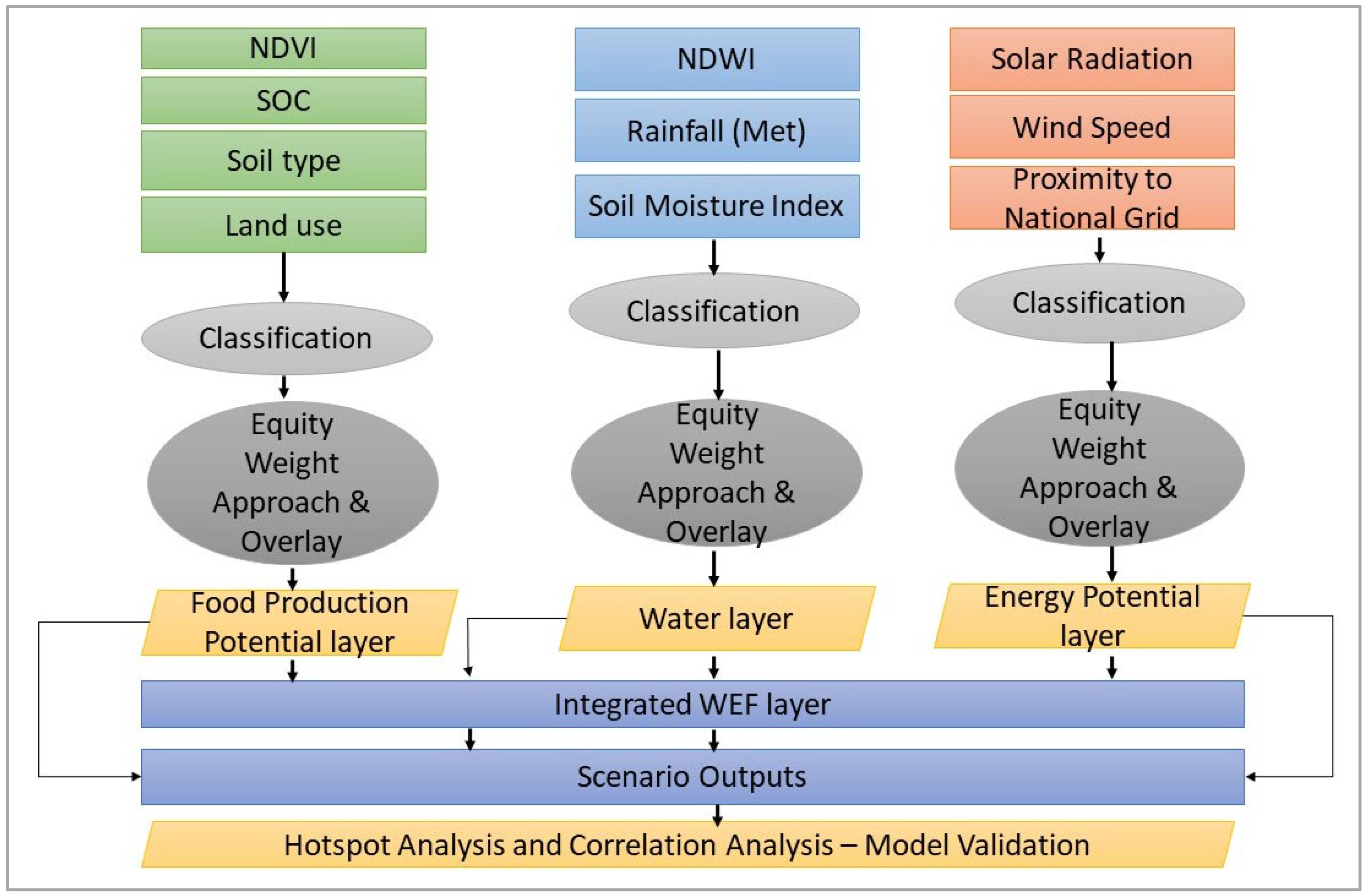
The WEF nexus-related models that were generated can be divided into different categories such as scenario-based assessment, integrated assessment modeling, decision support, and data-based models [23] (Namany et al., 2019). This study falls under the category of scenario-based assessment and modeling to assess the WEF interconnections by integrating biological, physical, climatic, and infrastructural parameters through classification and spatial analysis. The overall framework is presented in Figure 2. This study assesses the WEF nexus interlinkages for a sustainable paddy cultivation system. The spatial datasets representing food, water, and energy resource indicators were collected and processed in a GIS environment. The food-related indicators (NDVI, soil organic carbon, soil type, and land use), water indicators (NDWI, rainfall, and soil moisture index), and energy indicators (solar radiation, wind speed, and proximity to national electricity grid) were classified to generate standardized suitability layers. Each of the layers were combined using equal weights to generate an integrated WEF layer for the study area. As the model output, the functions were executed using the raster calculator in ESRI (Redlands, CA, USA) ArcGIS 10.7.1 software. To validate the model hotspot analysis for the primary layers and the model outputs, they were compared using band statistics and Pearson correlation. This integrated approach further enabled the identification of optimal, adaptive, and vulnerable areas to guide resource-efficient and climate-resilient agricultural policy planning.
According to [1] Cuthbert et al. (2022), it was found that WEF nexus tools are being developed with a current number of at least 46 tools and models, but the majority (61%) are unreachable to the intended users. According to the authors, a majority of about 70% lack capabilities such as geospatial features and transferability in spatial scale and geographic scope. Only 30% of the tools are applicable at the local scale [1] (Cuthbert et al. (2022). To address that issue, this study mainly features and is built around the geographic scope and is transferable in spatial scale. Also, the model was applied to a local scale and could change according to the desired region. The significance of this research is that this model can be altered to change to any local scale or desired parameters, and it can be changed according to end users’ interests without any difficulty.
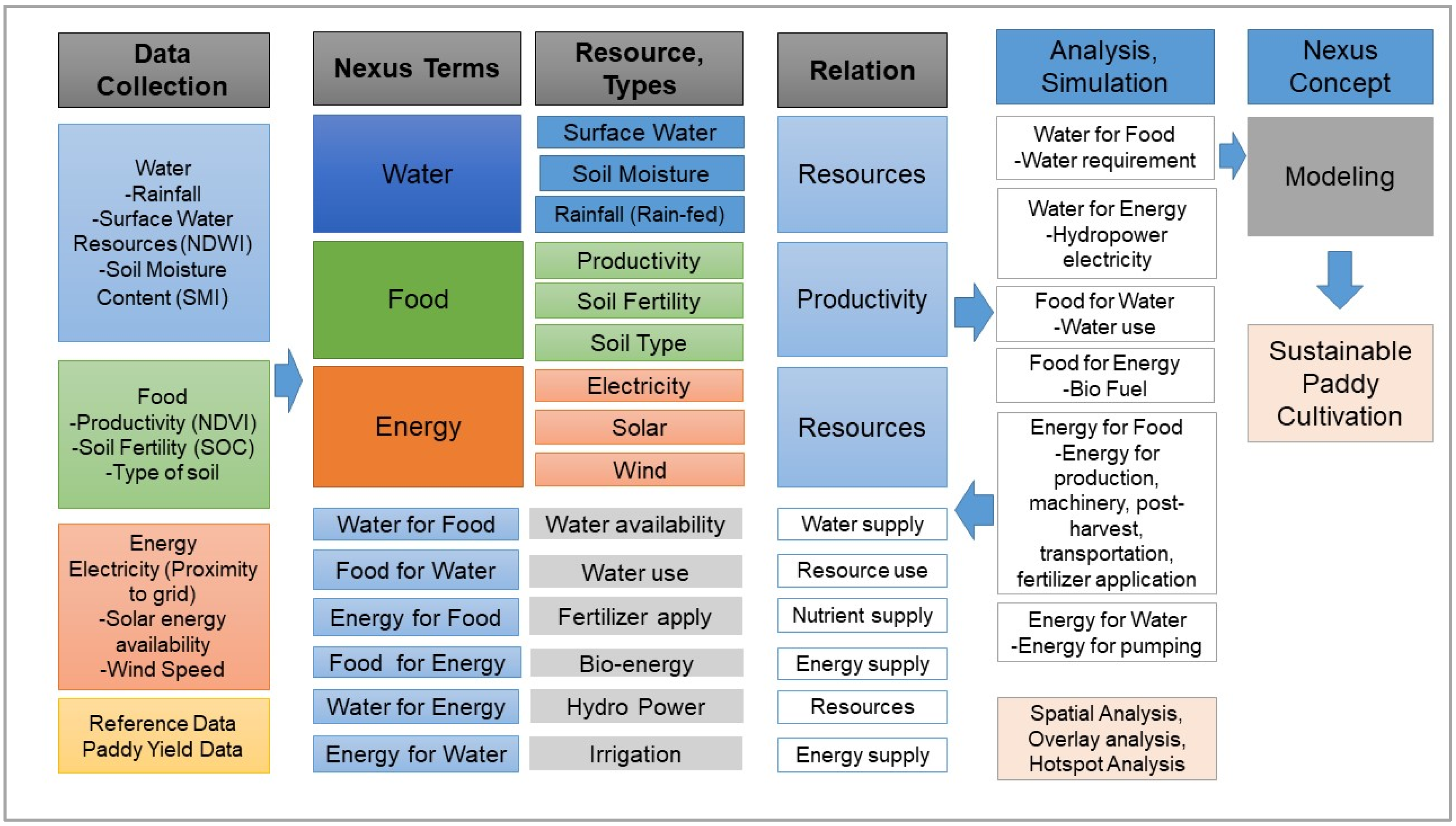
Figure 3 shows a diagram of the conceptual framework used for modeling the WEF network in the study. It was structured around five main components: data collection, nexus terms, resources, interrelationships, and analysis simulation outputs. In the phase of data collection, the data were collected under three core components, water, energy, and food. These data reflected different aspects that would influence the final output. The interrelationships among the components were then defined using the resource-based interlinkages essential for paddy cultivation. Mutual interdependencies among the water, energy, and food components indicate where each element relies on the others for efficient functioning in the study scope. These interdependencies are illustrated in the central section such as water for food, food for water, energy for food, food for energy, water for energy, and energy for water. For instance, water for food represents irrigation requirements for crop growth, whereas food for water reflects the use of agricultural land management practices that influence the water retention and soil moisture. Energy for food indicates the energy needed for agricultural operations such as pumping of water, farm mechanization, fertilizer application, and post-harvesting processes. Food for energy refers to biomass or bio-fuel production. Water for energy includes hydropower generation, and energy for water represents the electricity required for water extraction and distribution. These interactions demonstrate the nature of resources, that is, how changes in one component directly affect the others, defining the main principle of the WEF nexus concept. Analytical methods that were applied to this study included spatial overlay, hotspot analysis, and modeling.
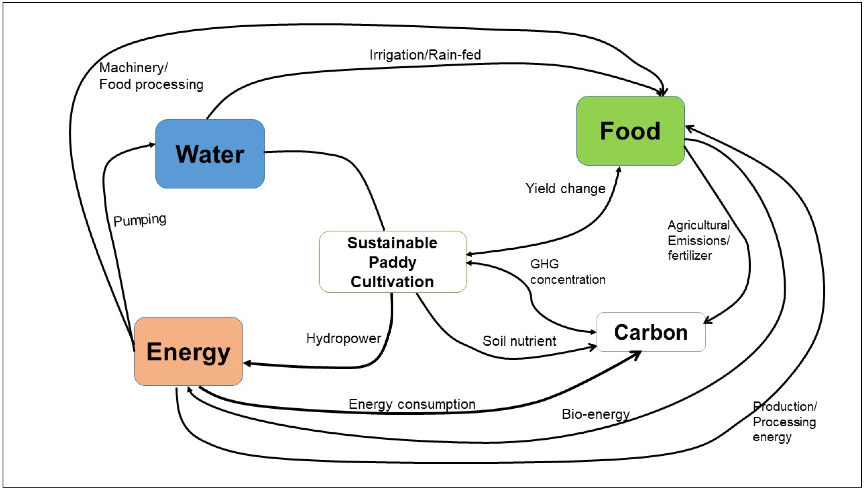
Figure 4 presents a schematic diagram of this study. It also highlights the dynamic and interdependent relationships among the WEF components. The arrows show the connections existing in the WEF system in paddy cultivation within the scope of this study. The diagram shows the spatial interconnections between different components acknowledged in this study. It highlights the feedback cycles, along with the dynamic and interdependent relationships among water, energy, food, and carbon (WEF-C) within sustainable paddy cultivation. The arrows represent the direction and the effect of each component on the others, demonstrating both the input and resulting outputs. The cycle shows water and energy inputs required for irrigation, water pumping, and farm machinery operations. Crop production (food) enters the system through changes in yield in a loop, with agricultural emissions influencing the carbon dynamics. Carbon and soil nutrient levels affect the crop productivity, which helps to create another feedback loop. Energy production (e.g., hydropower and bio-fuel) links back to the water and food components by completing the WEF cycle. These interconnected flows illustrate how scenario variations exist in a WEF system, enabling a comparative analysis under various modeled scenarios.
The diagram in Figure 5 illustrates the interactions of the WEF system of this study. These interactions can be displayed in a casual loop diagram [24] (Uddin et al., 2023). The interactions, such as water availability, are positively influenced by factors such as precipitation, and this positively impacts the food production potential and hydropower generation. Energy sources such as solar energy and wind power contribute to energy generation but do not contribute to GHG emissions [25] (Paraschiv & Paraschiv, 2023). SOC is a major reservoir of carbon in an ecosystem. When the soil is disturbed in instances such as tillage, land preparation, overuse of chemicals such as fertilizers, and crop residue burning, the SOC is oxidized and released as CO2 to the atmosphere [26] (Ghimire et al., 2019). Also, fertilizer use contributes to increasing the food productivity, but it also leads to SOC degradation and increased GHG emissions [27] (Liu et al., 2025), showing the synergy and trade-offs involving the same component. The diagram in Figure 5 depicts both positive and negative feedback loops, indicating that any change in one component can cause an effect on the entire system. The data that were used to implement this study are summarized in Table 1.

2.3. Derivation of Remote Sensing Indices

Three primary indices are calculated to assess land and water conditions:
(a)
Normalized Difference Vegetation Index (NDVI)
The NDVI provides a quantitative estimate of biomass, vegetation health, and growth [32] (Rouse et al., 1973) and evaluates the vegetation status by measuring the difference between the near-infrared and red portions of the electromagnetic spectrum. The NDVI varies from −1 to +1, and the closer the value is to +1, the higher the density and better the vegetation conditions that can be expected. The NDVI can be calculated using the following equation by assigning the appropriate bands for the equation.
NDVI = (ρ(NIR) − ρ(RED))/(ρ(NIR) + ρ(RED))
where
ρ(NIR) = Near Infrared Band (0.85–0.88 μm); ρ(RED) = Red Band (0.64–0.67 μm)
(b)
Normalized Difference Water Index
Ref. [33] McFeeters (1996) proposed the NDWI in 1996, which separates water and moisture by measuring the difference between the near-infrared and green bands. The NDWI ranges from −1 to +1; higher values are attributed to a high water content, while a lower value is a sign of no water level [34] (Amani et al., 2020). The NDWI can be calculated using the following equation by assigning the appropriate bands for the equation.
NDWI = (ρ(NIR) − ρ(Green)/(ρ(NIR) + ρ(Green))
where
ρ(Green) = Green Band (0.53–0.59 μm); ρ(NIR) = Near Infrared Band (0.85–0.88 μm)
(c)
Normalized Difference Infrared Index (NDII)-based Soil Moisture Index (SMI)
The NDII-based SMI is a widely used method for agricultural and land use studies. It is used to assess the soil moisture content using satellite imagery, which can capture surface moisture conditions by analyzing the reflectance. The near-infrared (NIR) and shortwave infrared (SWIR) bands of the visual spectrum are used to calculate this using the following equation [35] (Mathivha & Mbatha., 2021). The SMI can be calculated using the following equation by assigning the appropriate bands for the equation.
SMI = (ρ(NIR) − ρ(SWIR))/(ρ(NIR) + ρ(SWIR))
where
ρ(NIR) = Near Infrared (0.85–0.88 μm); ρ(SWIR) = Shortwave Infrared Band (1.57–1.67 μm)

2.4. Construction of WEF Layers

2.4.1. Food Layer

To develop the food production layer, four indicators—NDVI, SOC, soil type, and land use—were selected. Each factor was considered to be contributing to agricultural production and land use, which helps to mask and identify the paddy cultivated areas. To evaluate the impact of environmental and soil-related factors on paddy yield, it is essential to consider multiple factors. The NDVI is a measure of biomass and vegetation health [36] (Zhao and Qu, 2024), but it does not consider the soil properties that influence the crop growth. SOC impacts the soil fertility, water retention capacity, and microbial activity [37,38] (Zhang et al., 2019; Petropoulos et al., 2025) in soil, which is vital for paddy production. The soil type provides an idea of key physical and chemical properties, such as texture, drainage capacity, and nutrient availability, affecting land suitability and water retention for paddy cultivation [39] (Minh et al., 2023). By combining these layers, the food production potential layer was developed.
Table 2 summarizes the classification process applied to the physical parameters used in this study to create the food layer. The parameters NDVI, SOC, soil type, and land use were categorized into five classification levels ranging from Very Low (1) to Very High (5). NDVI and SOC values were classified using the Jenks Natural Breaks method, to cluster the data into natural clusters in the distribution. Soil type and land use were categorized based on the literature-derived suitability for paddy cultivation. The four criteria were classified using the values in Table 2 to create the food layer.
In this research, the equity weights approach [47] (Munda 2024) was used to create the final food layer, where each criterion was assigned as having equal importance. Using equal weights is an acceptable and commonly used method when expert-based weighting is not possible or desirable. All factors were considered equally important to obtain the output [48] (Zhao et al., 2024). In this study, considering all factors equal is important to make policy planning and decision-making possible. As the model contains four criteria, each criterion was assigned 25%, summing to a total of 100%. The following equation was used to create the food layer.
Food layer = (“NDVI_class” * 0.25) + (“SOC_class” * 0.25) + (SoilType_class” * 0.25) + (LULC_class * 0.25)

2.4.2. Water Layer

To develop the water layer for the WEF nexus assessment, three key hydrological indicators were utilized: rainfall, Normalized Difference Water Index (NDWI), and Soil Moisture Index (SMI). These indices collectively represent the availability and distribution of water across the study area. Table 3 presents the classification process applied to the parameters used in this study to create the water layer. Each parameter, rainfall, NDWI, and SMI, was categorized into five classification levels from Very Low (1) to Very High (5) based on Jenks Natural Breaks classification to maintain the natural clusters in the distribution. Higher rainfall, a higher NDWI, and a greater soil moisture content contribute to greater water availability and correspond to high value classes, and conversely, the lower values correspond to lower classification values.
The three layers were standardized to a common scale and were combined using a ratio of 1:1:1 to ensure that each component equally contributed to the water layer. This method provides a balanced representation of both underground and surface water availability. The equal weights support an unbiased representation of the components, which helps to have a clear understanding of the distribution of water in the area. The water layer was built using Equation (5).
Water layer = (“Rainfall_class” * 0.3333) + (“NDWI_class” * 0.3333) + (“SMI_class” * 0.3333)

2.4.3. Energy Layer

The energy layer was constructed by integrating three indicators: the proximity to the national electricity grid, intensity of solar radiation, and wind speed.
Using the values above in Table 4, the indicators for the energy layer were classified. The proximity to the national grid was classified using the equal interval method (Table 3), which divided the values into uniform ranges. For solar and wind energy, the five classes were obtained using Jenks Natural Breaks classification. The three layers were normalized and combined using the equity weight approach. The following Equation (6) was applied in the raster calculator to generate the energy layer.
Energy layer = (“Proximity_layer” * 0.3333) + (“Solar_layer” * 0.3333) + (“Wind_layer” * 0.3333)

2.5. Spatial Overlay and Nexus Integration

The normalized and weighted layers for the water, energy, and food were combined by creating a composite index. The following equation was used to create the integrated WEF layer comprising the food, water, and energy layers.
WEF Integration = (“Food_layer” * 0.3333) + (“Water_layer” * 0.3333) + (“Energy_layer” * 0.3333)
The integrated WEF layer reflects balanced contributions from all three components.

2.6. Scenario Creation

To develop the spatial model, in order to assess the interlinkages within the WEF nexus of the NCP, raster calculation and spatial modeling were used. Multiple scenarios were formulated (Table 4) to examine the synergistic and trade-off relationships within the WEF components. Each scenario was developed using equations with weighted raster layers to generate the expected outputs. The scenario-based modeling approach was used to identify the hotspots and coldspots, highlighting the resource availability in NCP. The scenario-based modeling approach enabled the identification of spatial hotspots where optimal conditions for water, energy, and food resources co-exist, and also the areas where resource constraints exist (Table 5).
Table 4 shows the equations that were used to create the scenarios using the Raster Calculator option in ArcGIS Desktop 10.7.1 software. The raster layers were in the WGS 1984 coordinate system; therefore, to calculate areas, the units were converted to meters.

2.7. Hotspot Analysis and Model Validation

To validate the developed WEF nexus model, a hotspot analysis using the Getis-Ord Gi* statistical tool [52] (Chakravorty, 1995) was performed to identify the statistically significant hotspots and coldspots. The Getis-Ord Gi* hotspot analysis is a statistical method that was used to identify the clusters of high and low values in spatial data. It calculates a z-score for each feature in the context of its neighbors, indicating whether that part of the feature has statistically significant high values (hotspots) or statistically significant low values (coldspots), to recognize the spatial patterns [52] (Chakravorty, 1995). These hotspot layers were administered to the extracted data in this study, the three primary WEF layers: water, food, and energy. These hotspot layers were subjected to a calculation of the pixel-wise Pearson correlation coefficient [53] (Guan et al., 2024) for scenarios 2, 3, and 4 (Table 4) to compare those and obtain the correlation value. Both raster layers were standardized to a common scale (0–1) to assess the level of agreement in the modeled outputs and the extracted data. For quantitative validation, band statistics including the mean, minimum value, maximum value, and standard deviation were also computed using the band statistics tool in ArcGIS to further validate the results. Overall, the validation framework integrated the visual hotspot comparison, descriptive raster statistics, and correlation analysis to ensure the robustness and the accuracy of the model. However, the model was validated internally using hotspot analysis of the same datasets, which confirmed that the spatial consistency and external validation with independent datasets remain a limitation.

2.8. Carbon Footprint Calculation

The total GHG emissions from paddy cultivation in the NCP were estimated by combining the CH4 and N2O emissions. The CH4 emission intensity for Sri Lankan paddy cultivation was reported as 4.77 tCO2eq ha−1 yr−1 [21] (Rathnayake and Mizunoya, 2023). To incorporate N2O emissions, an IPCC Tier 1 emission factor of 1.25 kg N2O-N ha−1 yr−1 [54] (Akiyama and Yagi, 2005) was applied. This value was converted to total N2O emissions using the molecular weight ratio of N2O to N2O-N (44/28) and was multiplied by the global warming potential (GWP) of N2O, 298 [55] (CCS, 2016), to obtain results in CO2 equivalents.

3. Results

The results of resulting raster layers are described below. All scenario outputs in raster format were produced by combining input datasets of different original spatial resolutions (e.g., WorldClim layers, Landsat satellite data). In the raster overlay process, ArcGIS automatically resamples inputs to a common working resolution, which results in different pixel sizes for raster outputs; hence, different pixel sizes for scenario outputs were experienced. These pixel sizes reflect the processing resolution required for each scenario output. For presentation purposes, all final maps were standardized to the same layout scale.

3.1. Primary WEF Layer Outputs

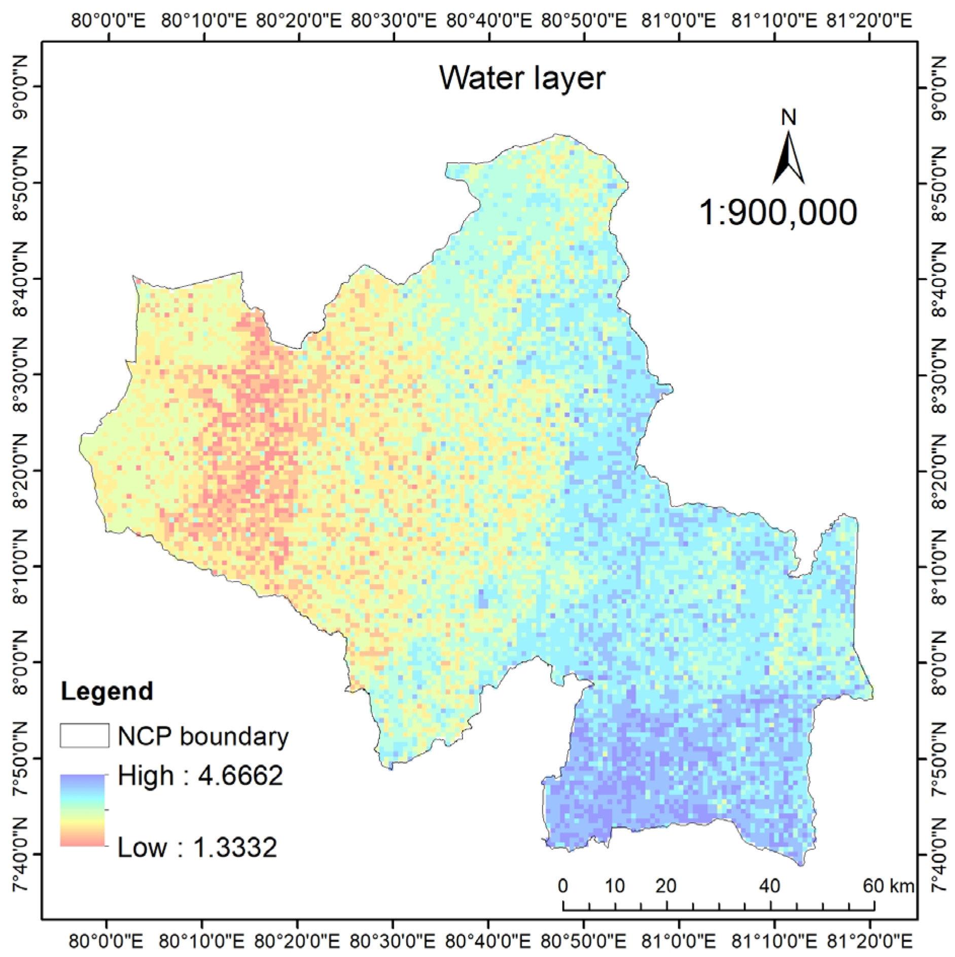
The water layer (Figure 6) shows the water availability in the NCP that could be utilized for paddy cultivation. Areas with high water availability are represented in blueish tones, and they were mainly concentrated in the eastern and southeastern regions. It could be said that, in these regions, adequate rainfall, favorable soil moisture conditions, and sufficient surface water exist. In contrast, the areas with low water availability were depicted in reddish to yellow shades, which were evident mostly in the southwestern region, reflecting areas with low water availability.
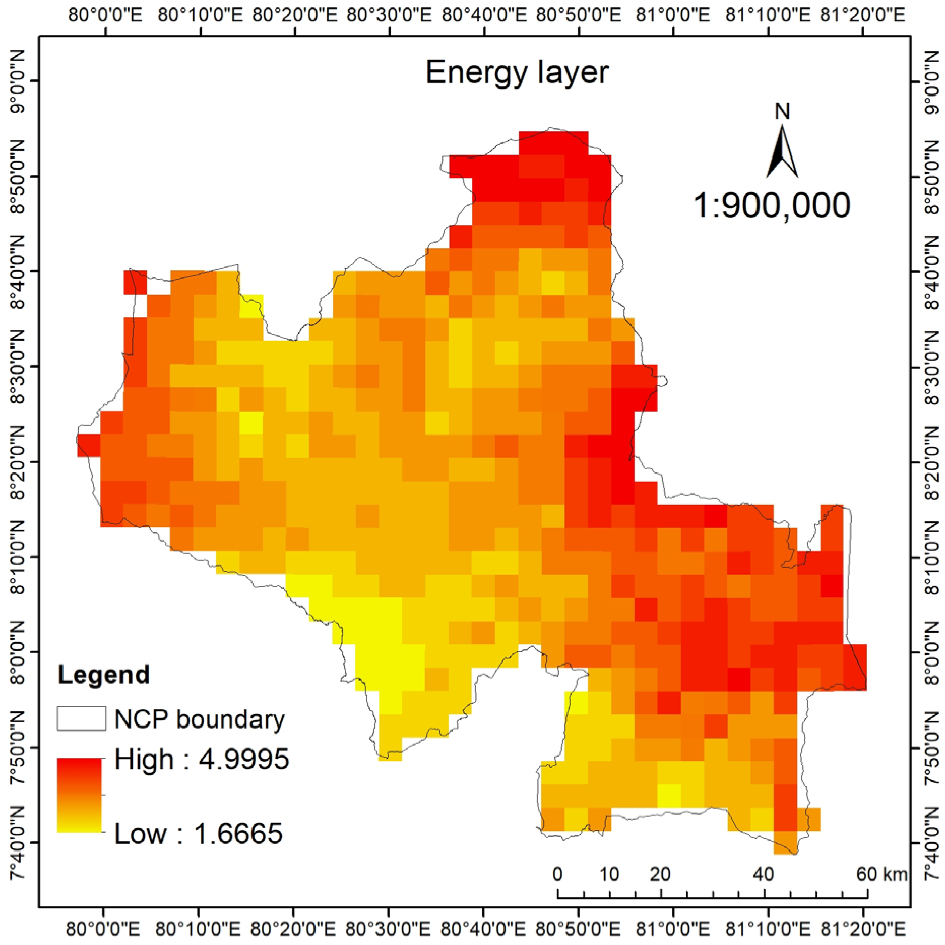
The energy layer in this study (Figure 7) is a composition of both renewable and conventional electricity that is distributed in the study area. The high-energy available zones were concentrated mainly in the central, eastern, and northwestern regions. The areas with low energy were visible mainly in the southern, southeastern, and southwestern regions.
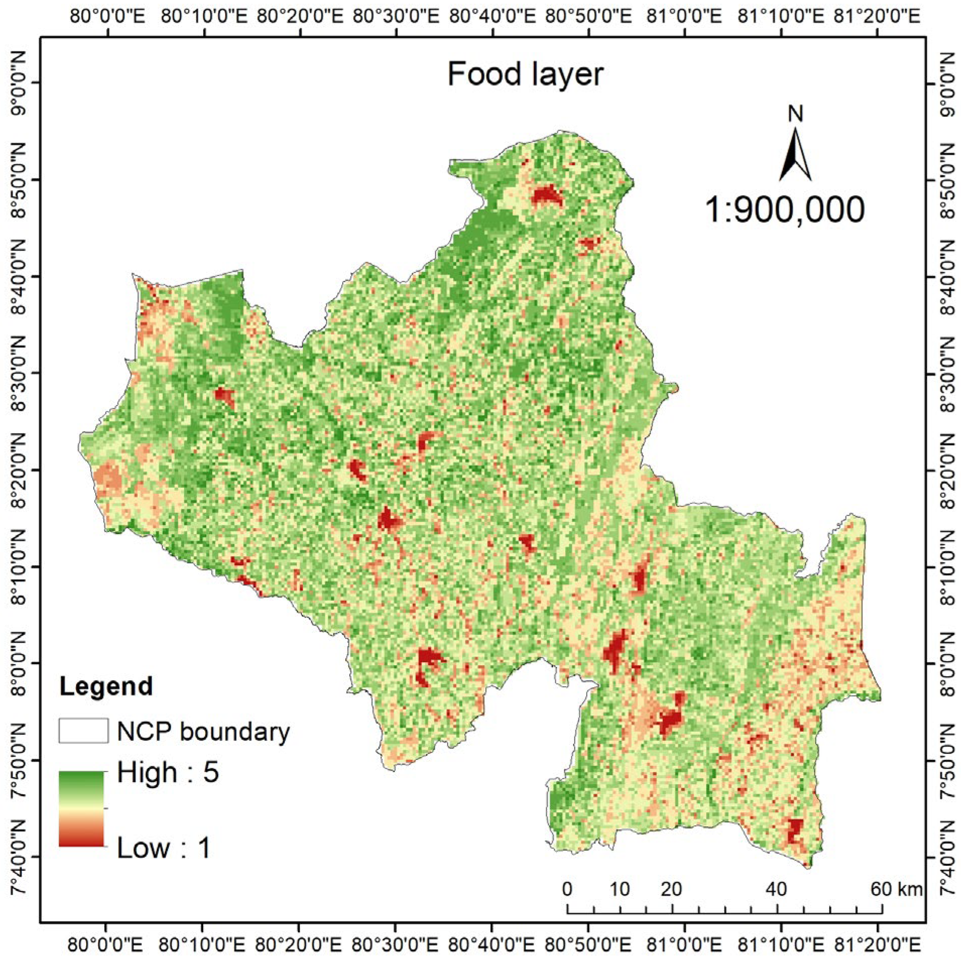
The food layer was depicted using Figure 8 below. The areas with high productivity potential of paddies are depicted in green, which were concentrated in the central and northeastern regions. These areas possibly consist of dense vegetation, fertile soil, and active cultivation zones. To extract these, as mentioned above, the soil type, NDVI, SOC levels, and land use were utilized. In contrast, areas with low food productivity represented, in a red to yellowish color, appeared scattered across the area.
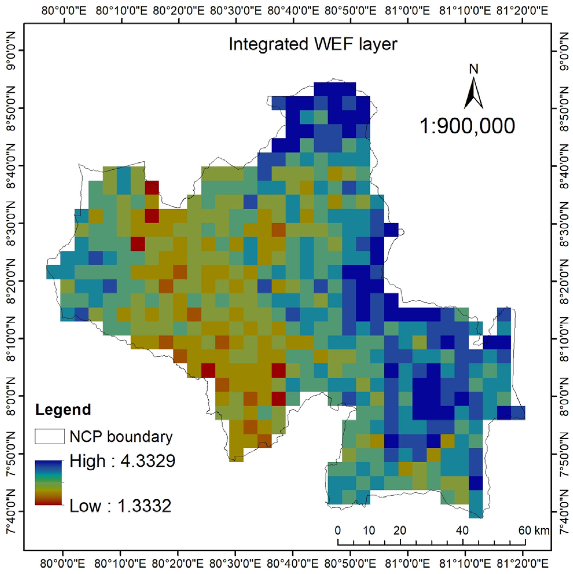
The integrated WEF layer (Figure 9) shows the spatial interlinkages among the three WEF components affecting paddy cultivation in the NCP. It is a representation of the water, energy, and food layers combined. High-WEF-potential zones, represented in blue shades, were prominent in the northeastern and southeastern parts of the province. On the other hand, the low WEF areas represented in red to yellow shades and could be observed mainly in the western and southwestern parts of the NCP.

3.2. Scenario Outputs

This study considered 12 scenarios that could occur in a paddy system under the WEF concept. The results obtained from the model are referred to as scenario outputs.
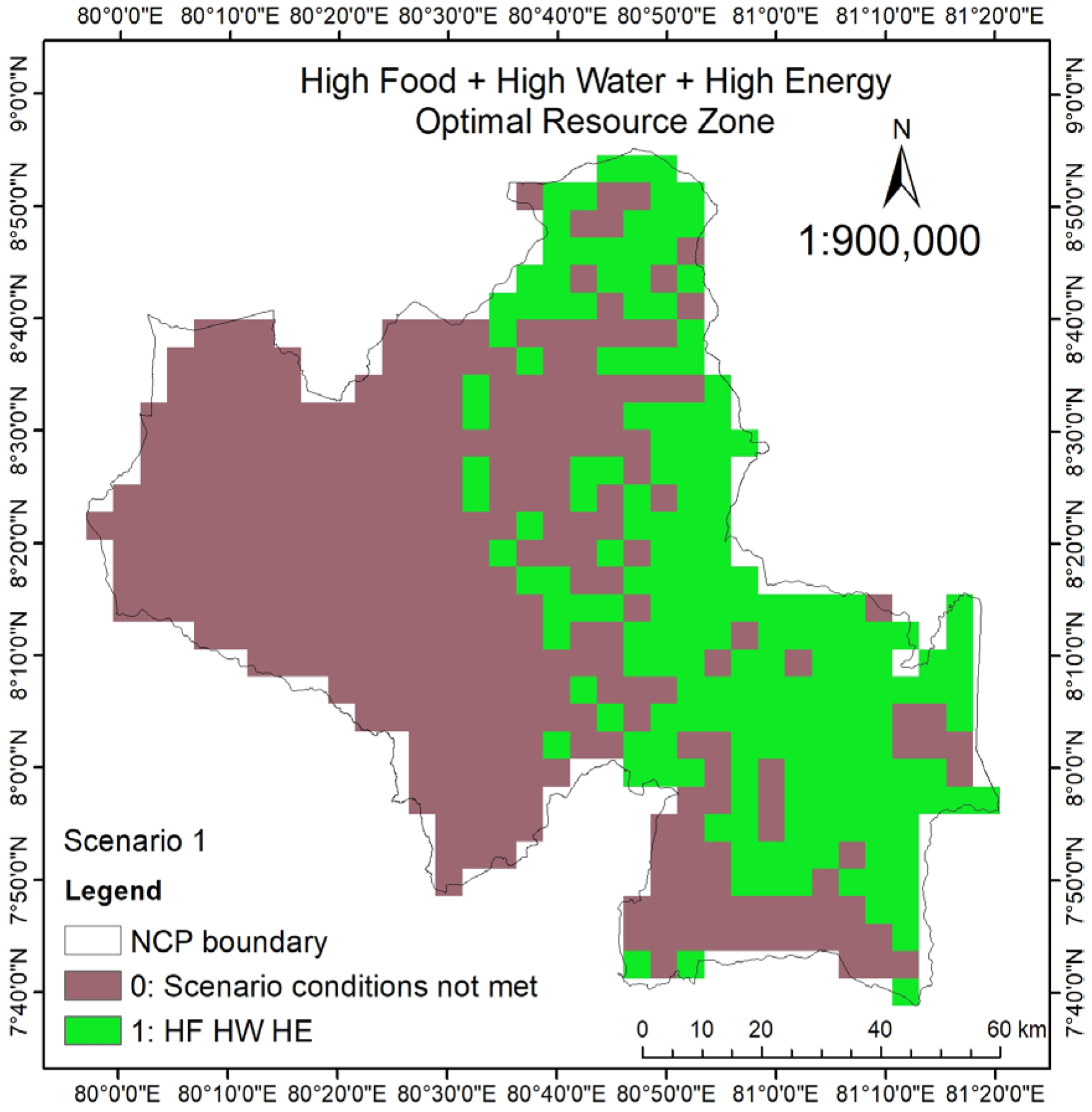
Scenario 1, depicted in Figure 10, represents the zones with optimal resources; it delineates the regions where paddy productivity, water availability, and energy access are at high levels. These optimal regions, zones with High Food + High Water + High Energy, are highlighted in a green color, in the northeastern, eastern, southeastern, and central areas of the province. The calculated area for the positive areas of WEF was about 371,443.60 ha. The area that did not fall under optimal WEF conditions was calculated as approximately 651,548.60 ha, which highlights the importance of enhancing the WEF conditions in the region for sustainable paddy cultivation.
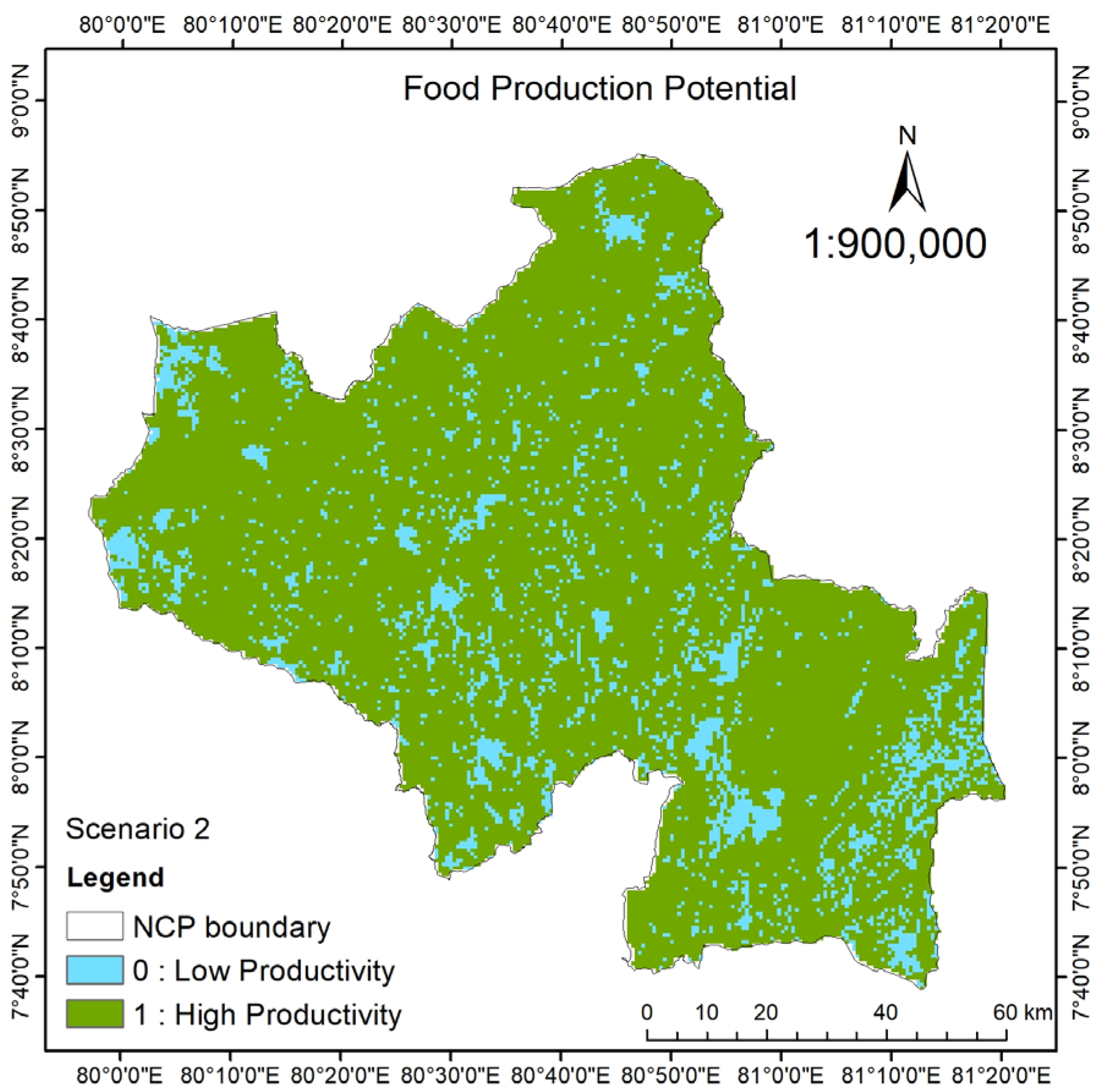
In scenario 2 (Figure 11), high-productivity zones were highlighted and extracted. The area for high food productivity was calculated approximately as 917,148.02 ha, and the area for low productivity was calculated as 134,966.58 ha. The low-production areas were scattered across the region in a pocket-like distribution, especially in the northwestern and southern margins, possibly due to available irrigation tanks and possible low-productivity areas.
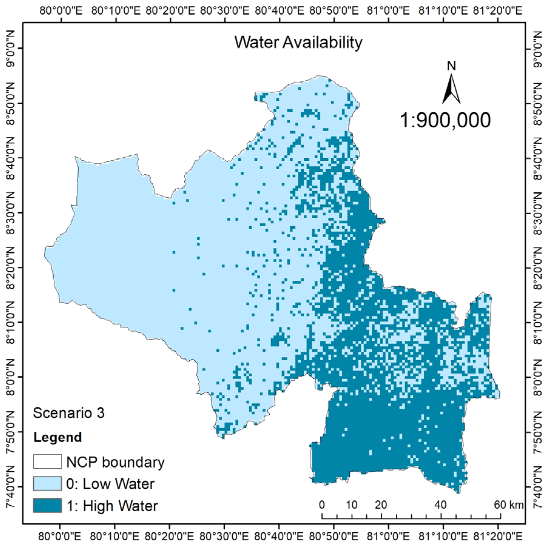
Scenario 3 (Figure 12) represents the spatial distribution in water availability, which was derived from the water layer. The high-water-available areas were primarily concentrated in regions like the eastern and southeastern zones of the NCP, with an area of about 359,079.71 ha. The low-water areas were dominant in the northwestern and central regions, indicating low soil moisture availability. These low-water zones highlight the trade-offs of hydrological conditions and have an area of about 696,957.90 ha as per calculations.
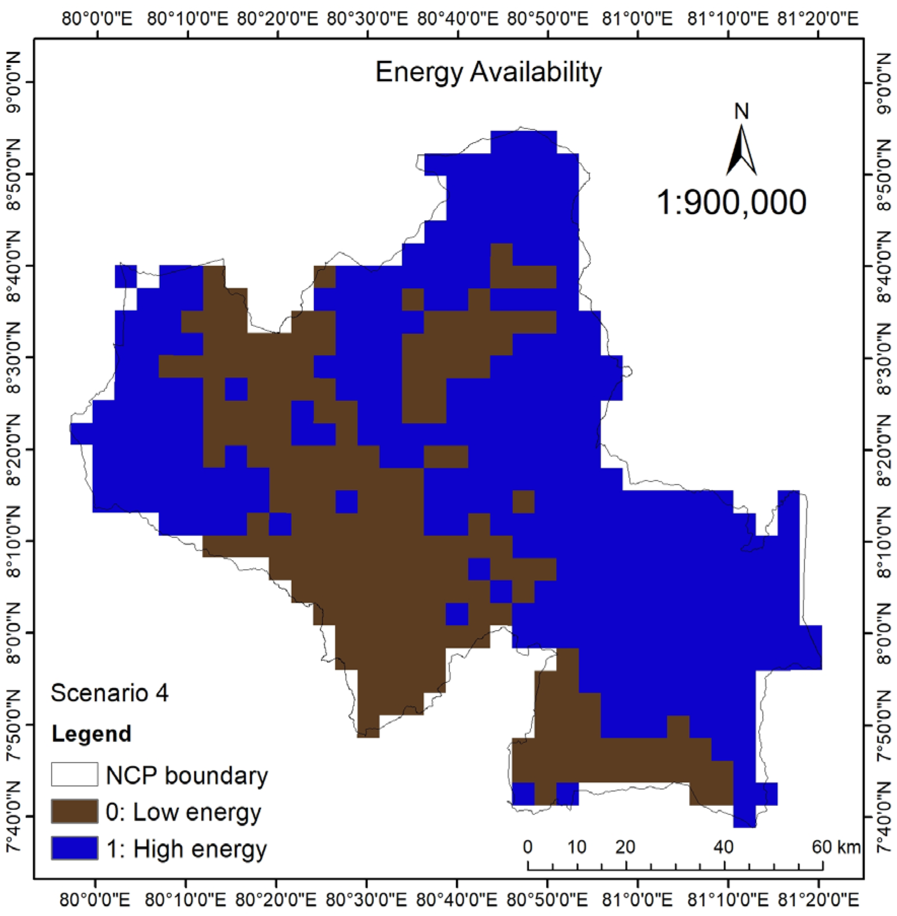
The potential energy scenario (Figure 13) represents regions with high and low energy availability. High-energy areas were clustered in the eastern and southeastern areas. The area calculated for high energy availability was approximately 665,300 ha. On the contrary, low-energy-potential zones were dominant in the northwestern and central regions. The area calculated for low energy was approximately 392,567.78 ha.
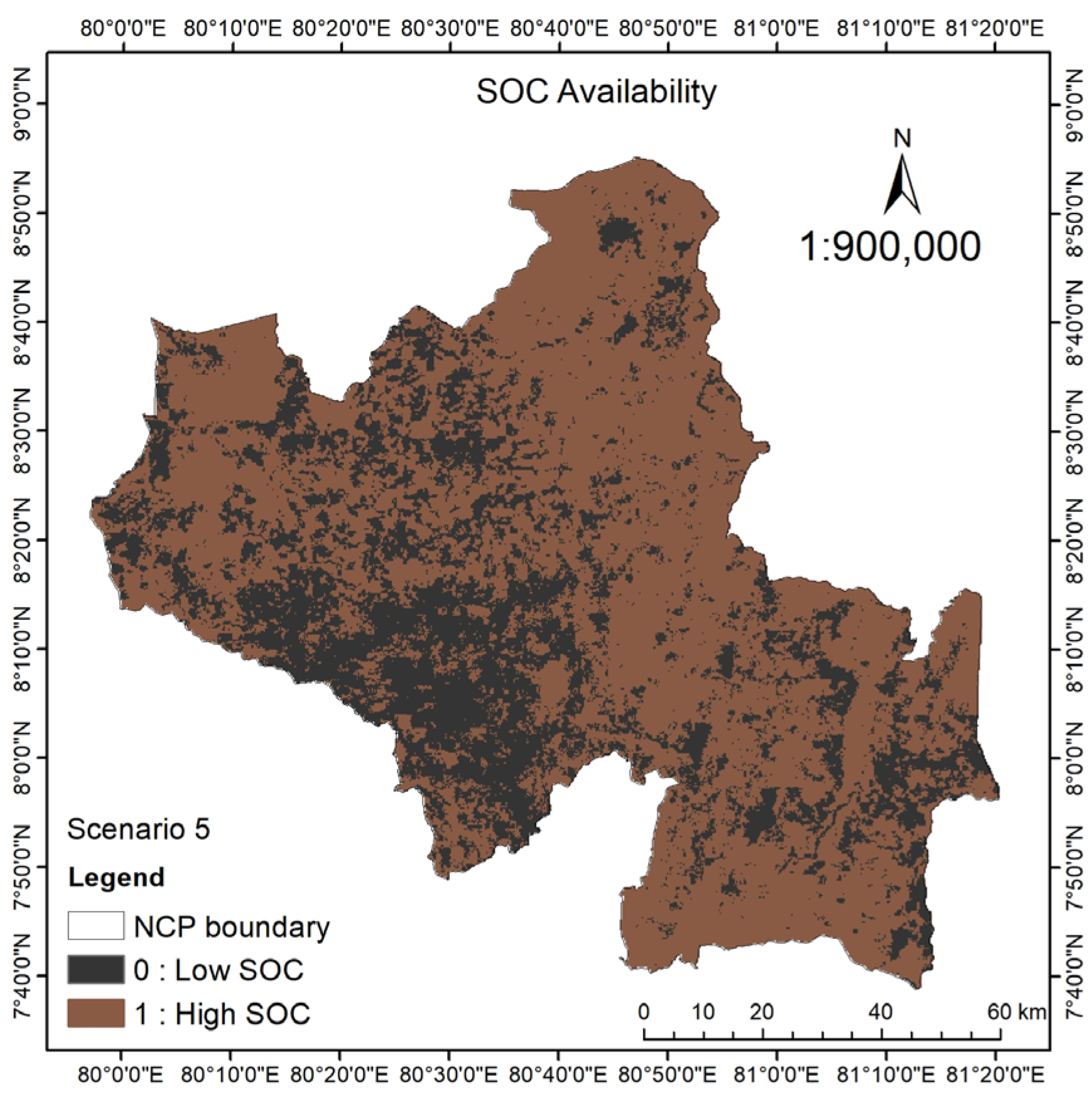
Scenario 5, representing SOC availability (Figure 14), illustrates the spatial distribution of SOC content in the NCP. The areas with high SOC were mainly distributed in the northern, eastern, and western regions, but they were not evenly distributed. The area calculated for high SOC availability was 746,336.53 ha. The central and southwestern regions showed relatively lower SOC levels. The area calculated for low SOC availability was approximately 335,998.58 ha.
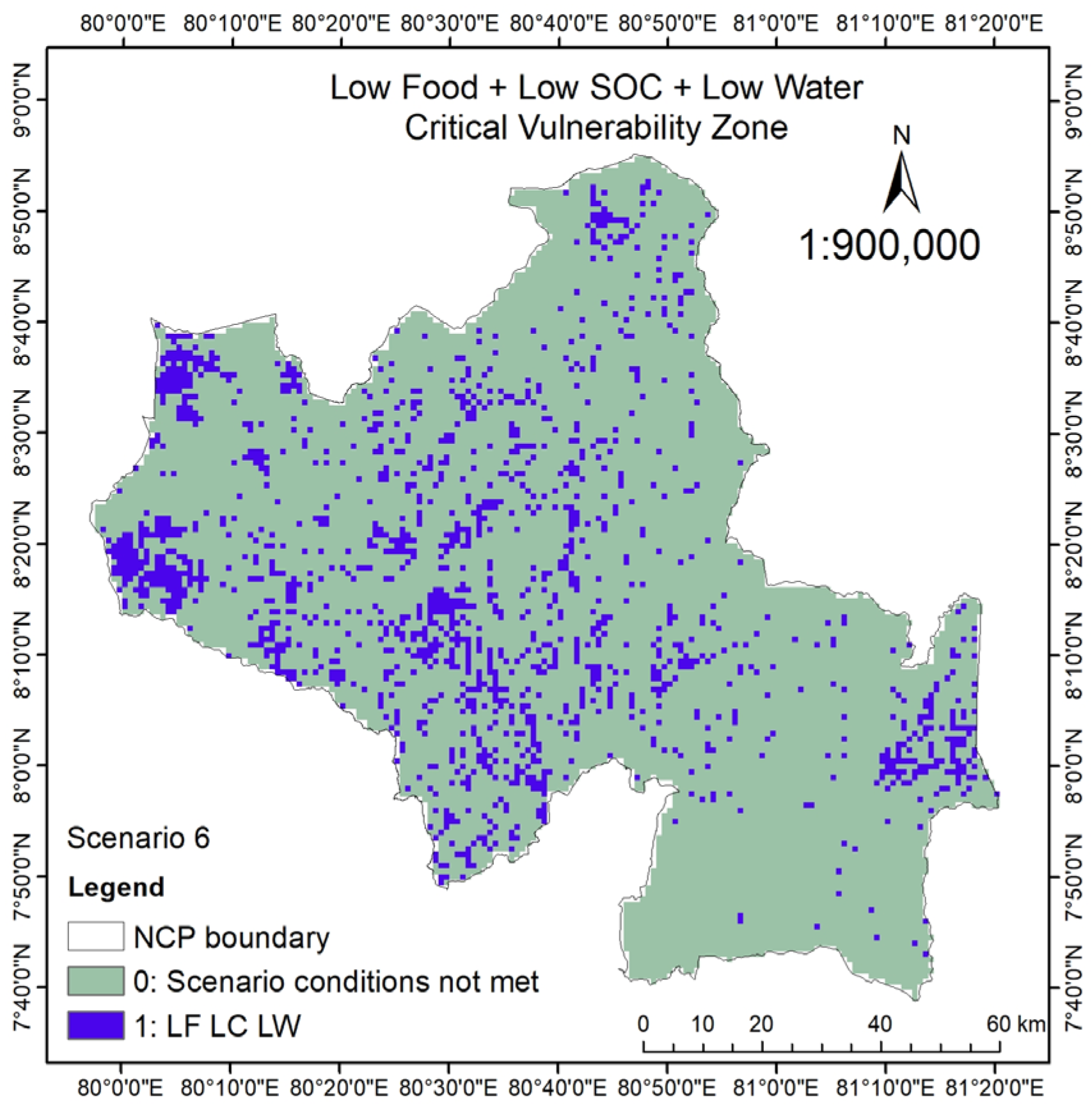
Scenario 6 (Figure 15), which contains Low Food + Low SOC + Low Water availability, identifies the regions with multiple resource limitations simultaneously. The areas marked in ‘purple’ tones indicate the regions with the above triple resource limitation, which has an area of approximately 127,798.05 ha. The area that does not agree with the conditions of the scenario was calculated as approximately 917,386.40 ha.
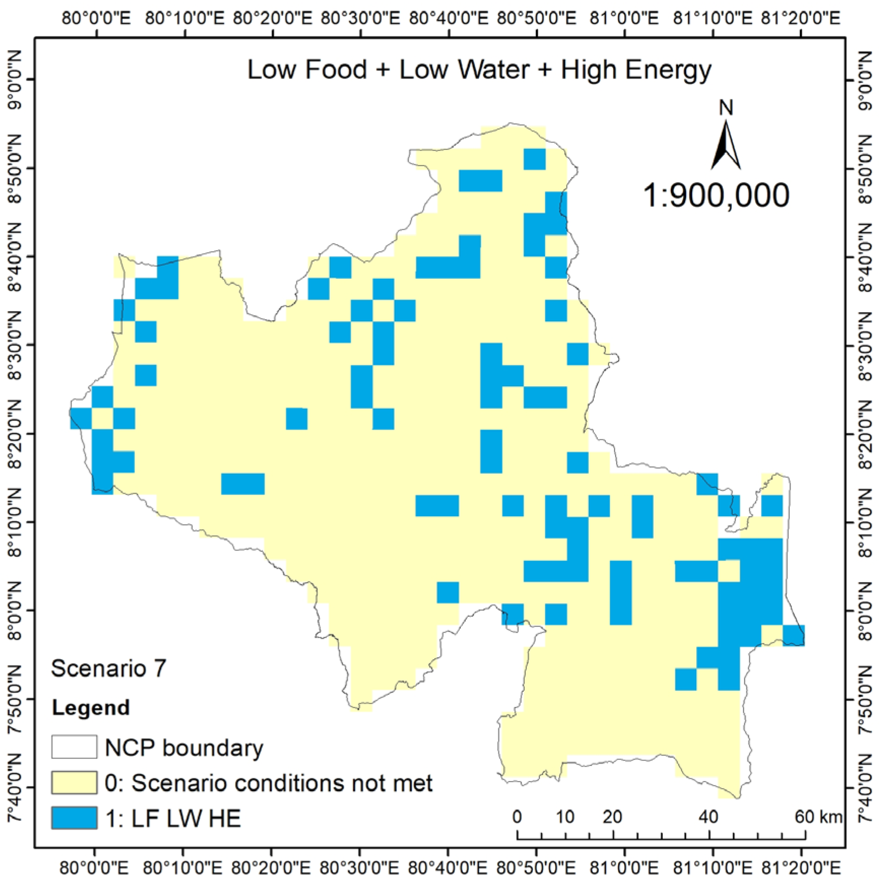
Scenario 7 (Figure 16) identifies areas with Low Food + Low Water + High Energy, where agricultural productivity and water availability are low, but potential energy availability is high. The blue zones, which have an area of approximately 190,085.45 ha, identify the areas where energy is not a limiting factor for low agricultural productivity but is possible, which could be due to the limited water availability or other issues such as low fertility or land degradation. The area that does not agree to the scenario was approximately 857,450.69 ha.
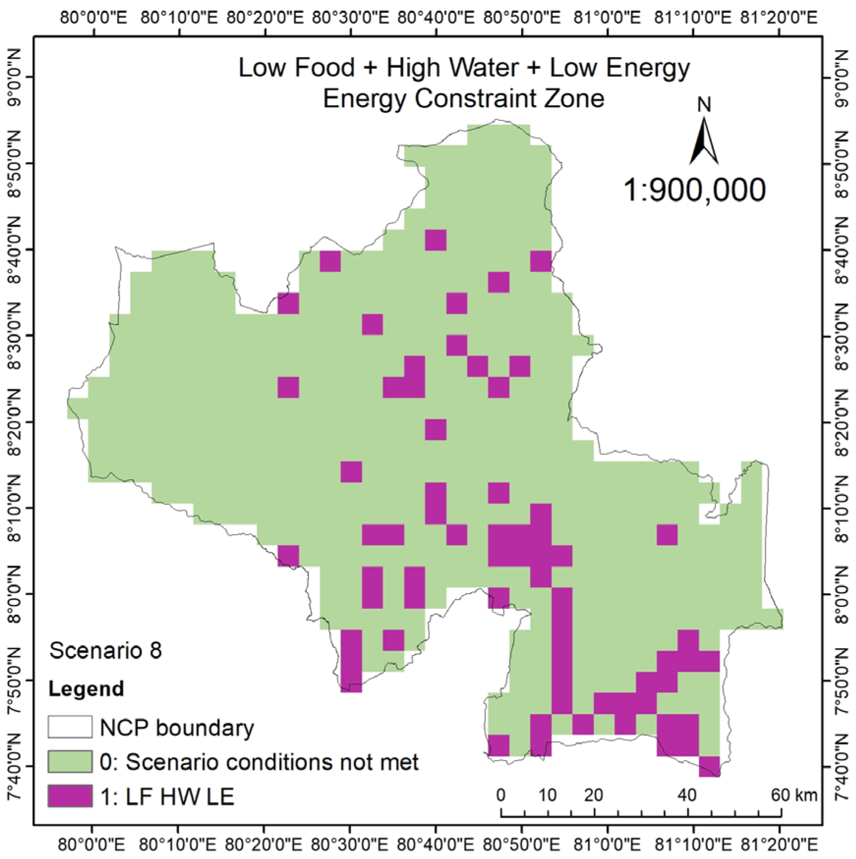
Scenario 8 (Figure 17), which was classified as the energy constraint zone, identifies regions within the NCP where the available water is high, but energy and food productivity are low. The areas where Low Food + High Water + Low Energy were spread in the southern and central parts of the NCP formed an area of approximately 138,022.75 ha. The area that does not agree with the conditions of this scenario was calculated as approximately 884,969.44 ha.
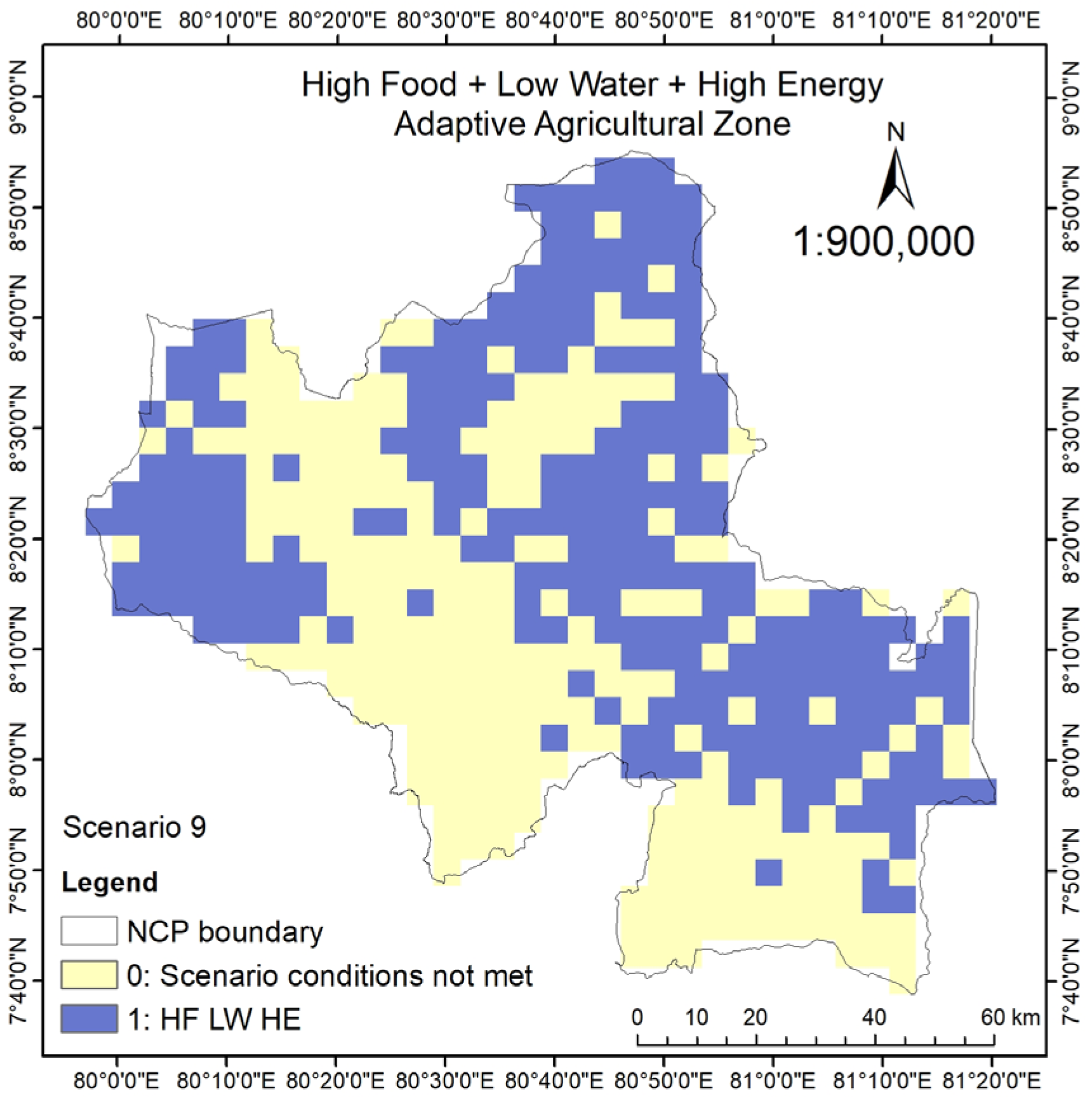
Scenario 9 (Figure 18) represents the areas in the NCP with High Food + Low Water + High Energy, where agricultural productivity remained high despite the low water availability, which was supported by the high energy availability. These areas demonstrate how sufficient energy access could overcome the limited water availability in an agricultural system. The blue areas, of around 493,228.38 ha of area, highlight the regions that are possibly able to overcome the water scarcity to have high production. The area that does not agree with the conditions of this scenario was 529,763.81 ha.
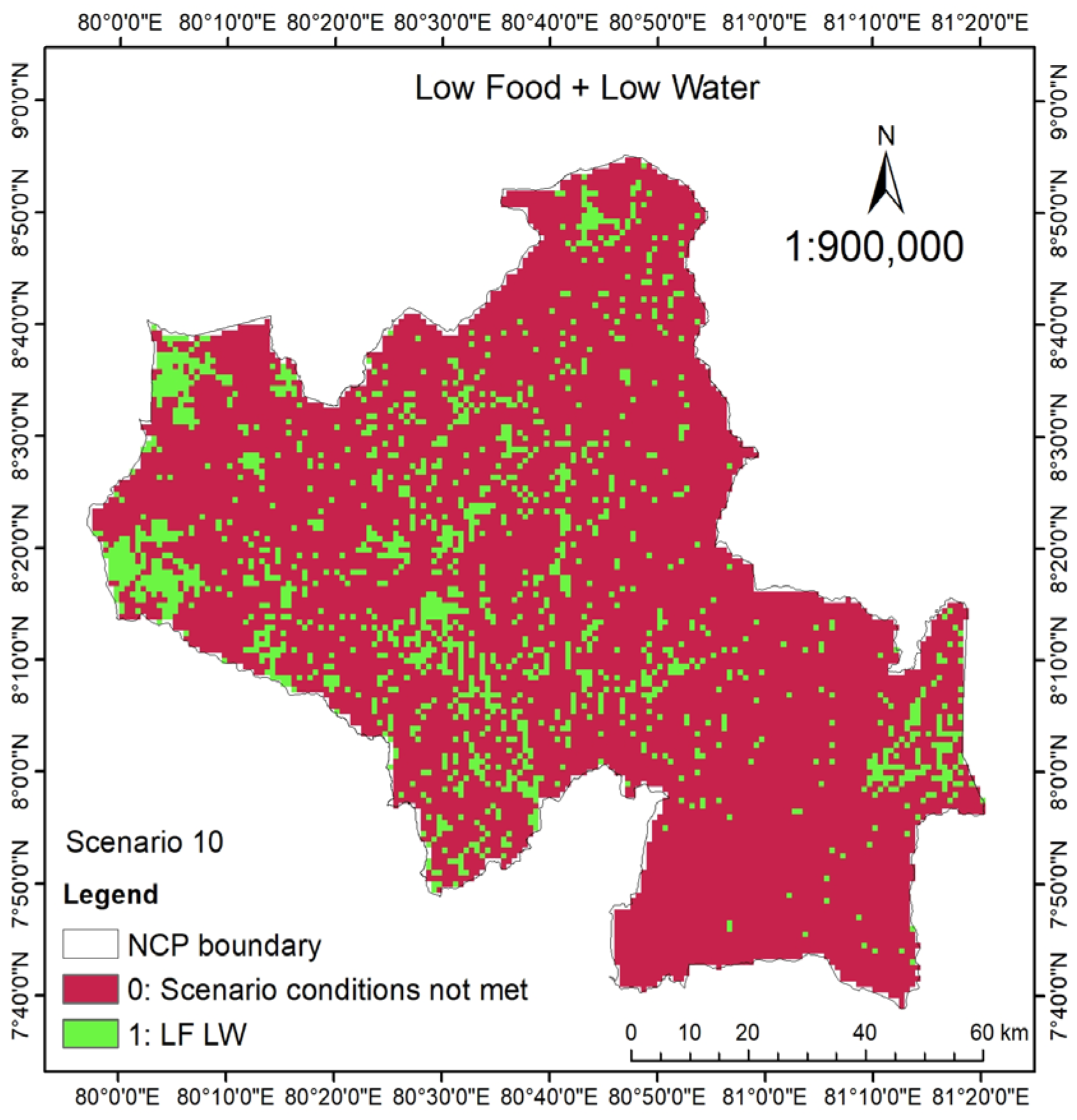
Scenario 10 (Figure 19) depicts the regions that have both low productivity and low water availability. Low Food + Low Water areas, represented by the green patches distributed among the region, indicate where productivity can be affected by the low water availability. The area covered by Low Food + Low SOC was around 137,389.21 ha approximately. On the map, the areas were mainly distributed across the central and the western regions of the province. The area that does not agree with the conditions of this scenario was around 908,552.43 ha.
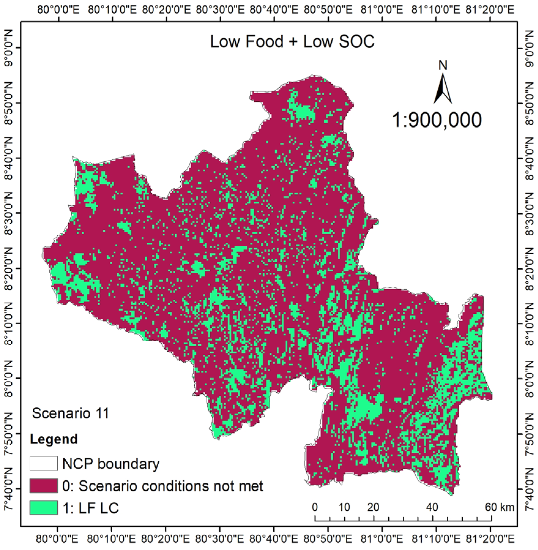
Scenario 11 (Figure 20) is representing areas with low paddy productivity and low SOC levels. Low Food + Low SOC areas are distributed around the area in a scattered form. Those spatial patterns reveal that these areas are mainly concentrated in the southern and southeastern parts, but are substantially spread across the entire province, as represented in green patches. The area calculated for Low Food + Low SOC was approximately 234,008.35 ha. The area that does not agree with the conditions of this scenario was approximately 818,106.25 ha.
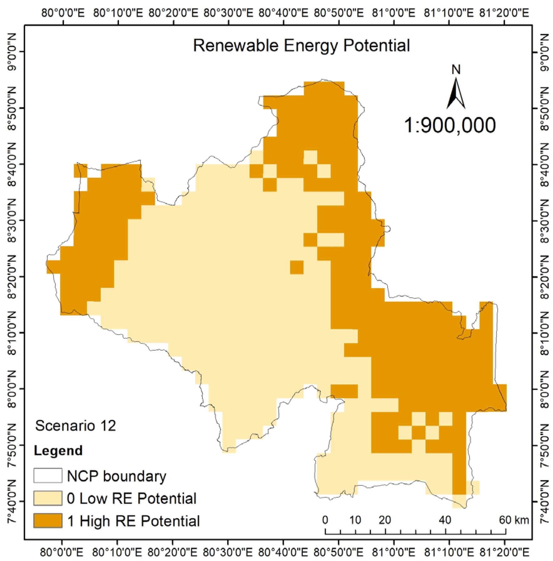
Scenario 12 (Figure 21) highlights the areas with high renewable energy availability. The eastern, southeastern, and northwestern regions were highlighted as areas with both high intensities of solar radiation and wind speed. The area calculated for high renewable energy was approximately 601,248.55 ha. The area for low renewable energy availability was calculated as 456,618.32 ha.

3.3. Model Validation

3.3.1. Model Validation: Correlation Analysis Between Hotspot and Scenario Layers

To assess the accuracy of the model, a pixel-based correlation analysis was performed between the hotspot layers (representing the extracted data) and the corresponding scenario layers (representing the modeled outputs). The validation results are summarized below in Table 6, Table 7, Table 8 and Table 9. Using Pearson’s correlation “r” enables us to investigate how closely the modeled outputs and the extracted data are aligned. A positive correlation with higher values reflects the model’s reliability and spatial coherence. Moreover, the Pearson coefficient is a widely used method to validate raster-based GIS model outputs, to identify the linear relationships.

3.3.2. Interpretation by Water Component

The Pearson correlation coefficient (r = 0.737) (Table 6) indicates a strong positive correlation between the hotspot and scenario layers for the water layers where p > 0.001, and the value was statistically significant. This result demonstrated that both layers show similar spatial patterns, confirming the high model accuracy and reliability. The covariance values (0.089–0.122) further confirm these results. The mean pixel values, 0.4532 and 0.5396, show close value ranges, which confirms the similar spatial behavior.

3.3.3. Interpretation by Energy Component

The validation results for the energy layers give a moderate positive correlation (r = 0.582) (Table 7). The value was statistically significant where p > 0.001. The covariance range (0.064–0.119) confirms that both layers vary together positively. This further confirms the validity of the model. The mean pixel values, 0.6818 and 0.4316, for the two layers, which have a closer range, show a strong spatial correspondence.

3.3.4. Interpretation by Food Component

The validation between food layers of hotspots and scenarios showed a moderate positive correlation of r = 0.273 (Table 8). The value was significant where p > 0.001. The mean pixel values for hotspots (0.578) and scenarios (0.940) indicated that the scenario layer showed higher food productivity levels than the other. This correlation value generates a satisfactory level of agreement for validation purposes. The standard deviation values show how dispersed the pixels are from the mean value and the degree of variation between the hotspot layer and the respective scenario layer. The water layer (SD = 0.4977, 0.4984) and energy layer (SD = 0.4658, 0.4958) showed a strong, consistent variability, and the food layer (SD = 0.4938, 0.2378) displayed the close variability between the layers. These results further support the reliability of the model.

3.4. Carbon Footprint Results

To estimate GHG emissions associated with paddy cultivation in the NCP, CH4 and N2O emissions were quantified using IPCC Tier 1 emission factors and standard conversion procedures. Based on the reported total paddy cultivated area of approximately 200,000 ha in the NCP [56] (Department of Census and Statistics, 2025), the annual CH4 emissions (E_CH4) were calculated using an emission factor of 4.77 tCO2eq ha−1 yr−1 in Sri Lankan paddy lands [21] (Rathnayake and Mizunoya, 2023). Accordingly, the total CH4 emissions were estimated as
Total E_CH4 = 200,000 ha x 4.77 tCO2eq ha−1 yr−1 = 954,000 tCO2eq yr−1
To incorporate N2O emissions (EN2O), the IPCC Tier 1 default emission factor of 1.25 kg N2O-N ha−1 yr−1 [54] (Akiyama and Yagi, 2005) was applied. The N-based value was converted to total N2O gas emissions using the molecular weight ratio of N2O to N2O-N (44/28). N2O emissions were calculated as follows:
E _ N 2 O   =   1.25   kg   N 2 O- N   ha 1   yr 1   ×   44 28 =   1.96   kg   N 2 O   ha 1   yr 1
The resulting N2O gas emissions were then expressed in CO2 equivalents by applying the global warming potential (GWP) of N2O = 298 [55] (CCS, 2016).
E_N2O-CO2 eq = 1.96 kg N2O ha−1 yr−1 × 298 = 0.584 tCO2eq ha−1 yr−1
The total N2O emissions for the NCP were then calculated by multiplying the emission intensity by the cultivated area as follows:
Total E_N2O = 0.584 tCO2eq ha−1 yr−1 × 200,000 ha = 116,800 tCO2eq yr−1
As calculated above, the total N2O emissions from the paddy lands in the study area were estimated as 116,800 tCO2eq yr−1.
Combined total GHG emissions (E_CH4 + E_N2O) = 954,000 + 116,800 = 1,070,800 tCO2eq yr−1
As calculated above, the total GHG emissions from the study area were estimated as 1,070,800 tCO2eq yr−1. The resulting emission intensity for paddy cultivation of the NCP was 5.35 tCO2eq ha−1 yr−1. The final results suggest that the share of CH4 emissions is equal to approximately 89.09% (89%) and the share of N2O emissions is approximately 10.9% (11%) in the NCP.

4. Discussion

In Figure 6, it is shown that water layer areas with low water availability could be highly vulnerable to drought effects, especially during the Yala season, when the rainfall is comparatively limited. Identifying these regions could help to improve the irrigation infrastructure, to promote water availability for paddy cultivation, since a paddy requires a large quantity of water to cultivate rice.
In Figure 7, the low-energy areas highlight where an integration of hybrid energy solutions should be introduced to enhance the sustainable energy sources in the area. Energy is a vital component in any large-scale cultivation. Therefore, the availability should be sufficient. Using fossil fuels as energy could impact the climate change; therefore, considering renewable energy options is eco-friendly. The cost that is utilized for energy can be reduced by using renewable energy sources. Although the initial cost required to implement energy plants is higher, the cost of energy consumption can be reduced in the long run. In Sri Lanka, the cost of production is high when it comes to paddy cultivation. Therefore, there is a timely need to incorporate renewable energy.
In Figure 8, the red zones could be identified as water bodies when compared with land use, and the other regions could be due to degraded soils and less vegetation cover. The green areas, which were scattered across the area, could be of fertile land with good productivity. The other regions could be improved with soil fertility enhancement, organic matter management, and land rehabilitation.
In Figure 9, high-WEF areas, high water availability, high agricultural productivity, and optimal energy availability are coexisting. These regions highlight the synergistic effects of WEF components, which promotes sustainable paddy cultivation. The low-WEF areas can be identified as regions where WEF trade-offs among the three WEF components are existing. Multiple interventions, such as improved irrigation and renewable energy sources, could help to improve the paddy production in these regions. Improving the primary WEF components in these constraint areas could enhance the sustainability of the paddy cultivation in the area.
In Figure 10 scenario 1, it is shown that high-WEF regions would benefit from better hydrological conditions, reliable access to energy sources, and high productivity. Further, these areas can be identified as the areas with minimal resource stress. Also, these optimal zones act as a benchmark for sustainable resource availability and effective WEF nexus management demonstration. Maintaining these conditions, through better resource management, is essential to ensure long-term sustainability in the paddy cultivation in the DZ. The identified outputs from this scenario can be utilized as regions for demonstration and model areas for climate-resilient paddy cultivation and integrated resource management. Also, direct agricultural investment policies (e.g., mechanization subsidies, precision agriculture) to maximize productivity and establish benchmark sites could be introduced. Furthermore, implementing land use policies that avoid encroachment or land degradation in these areas could be prioritized.
With regard to Figure 11, scenario 2, the low-productivity areas enhancing the soil carbon content [22] (FAO, 2017), allowing site-specific nutrient management, and ensuring a sufficient water supply possibly could improve these areas, elevating them to high-production zones. This scenario highlights the importance of introducing policies such as rehabilitation of land and cultivation of marginal lands to reduce disparities in production. Similarly, prioritizing fertilizer subsidies, enhancing organic matter, and introducing precision agricultural practices in these low-productivity regions are equally important.
Figure 12, scenario 3 depicts the calculated area for low water; this area shows that most of the NCP has low water availability and therefore needs intervention. These regions could be improved by using methods such as rainwater harvesting, micro-irrigation systems, and tank rehabilitation, to ensure there is sufficient water availability during the changing climatic conditions. These areas could have better soil moisture conditions and a sufficient irrigation network. This scenario effectively indicates the importance of policies such as allocating government funds for modernization of irrigation systems, restoring tanks, and giving subsidies for micro-irrigation systems. Also, promoting climate-adaptive water management policies and rainwater harvesting methods at the farm level is important.
Figure 13, scenario 4 shows that high-energy areas could be adapted according to the need, for example, by introducing agrovoltaic zones or introducing solar-powered irrigation, while reducing the dependence on conventional energy sources. This requires implementing policies such as targeting low-energy regions for renewable energy expansion (solar, wind, hybrid systems), introducing policy incentives for agrovoltaic development, and improving off-grid irrigation systems. Also, reducing the dependence on fossil fuel-based agricultural operations is equally important to achieve sustainability.
Figure 14, scenario 5 depicts that the high-SOC zones possibly indicate regions with a better soil fertility and water retention capacity, considering the availability of SOC [22] (FAO, 2017). On the contrary, the areas with low SOC may require soil restoration methods like introducing organic matter amendments, mulching, and improved tillage to improve the soil health. This scenario is important to identify areas that need soil health improvements and to identify the areas with degraded soil fertility, to improve crop productivity before the onset of cultivation. This scenario highlights the importance of implementing soil restoration policies aimed at increasing soil SOC levels by using ingredients such as bio char and composting methods. Regulations regarding land degradation and protection of soil nutrients are another important factor that could fall under this scenario.
Figure 15, scenario 6 depicts that the areas agreeing with the scenario conditions could undergo thorough ecological resource stress with low productivity. The regions are concentrated in the northwestern and central parts of the province. These zones represent areas that need a high priority in restoring soil health and improving water availability in order to achieve high productivity. This could be improved by introducing land and water management practices and rainwater harvesting systems, improving irrigation facilities, and restoring soil health. This scenario highlights a critical tool to identify areas with WEF constraints that need immediate restoration interventions. When implementing policies for resource deficiency, these regions act as priority zones. Restoring these regions requires allocating government funds, conserving the soil and land to improve overall productivity, and introducing crop rotation practices and crop diversification policies.
Figure 16, scenario 7 illustrates that the area agreeing with this scenario demonstrates the potential for energy-driven adaptation, which could support the areas with limited water availability by introducing integrated water management, energy-efficient irrigation techniques, and renewable energy-based pumping systems. Overall, this scenario further highlights that although the energy access is sufficient, enhancing water availability and introducing proper soil health could improve agricultural productivity. Under this scenario, creating policies to optimize the water supply by means of renewable energy, and encouraging public- and private-sector partnerships for smart water–energy practices, could be considered.
Figure 17, scenario 8 shows the areas where the food production is potentially affected by the low energy availability. Therefore, these regions need interventions to promote the optimal energy availability in order to increase the sustainable paddy cultivation in the region. Increasing renewable energy use to reduce productivity loss due to low mechanization, and formulating policies for ensuring energy security for agricultural systems, such as the implementation of mini solar grid facilities by government funding or subsidies, are important policies that are being highlighted by this scenario.
Figure 18, scenario 9 shows that the limitation of water availability could add resource stress to the paddy cultivating regions, which could affect the productivity and the sustainability on a long-term basis. In this scenario, introducing improved irrigation policies, and regulations regarding ground water regulation and ground water recharge systems, and improving water use efficiency and precision agriculture to improve productivity, are highlighted.
Figure 19, scenario 10 conveys that improving the water availability, possibly by introducing rainwater harvesting systems, micro-irrigation systems, and improved irrigation systems, could mitigate these issues. Under this scenario, identifying areas with high-intensity irrigation requirements to protect food security at the national level is highlighted. Government-supported interventions regarding rainwater harvesting and water canal and infrastructural rehabilitation in the identified regions are important.
Figure 20, scenario 11 shows that the areas that agree with this scenario could be of poor soil fertility and reduced organic matter and may have been subjected to land degradation. Such conditions could limit the nutrient availability, soil health, and soil moisture retention capacity, which lower the crop yields and ultimately affect the productivity. Introducing soil health restoration practices, expanding financing schemes for soil carbon enhancement, and reducing soil degradation at the national level are important. This scenario helps identify such regions that need policies regarding soil carbon restoration.
Figure 21, scenario 12 depicts that the areas with high renewable energy are suitable for developing renewable energy infrastructure, by providing an opportunity to enhance rural electricity availability and agricultural mechanization, and the cost that would be consumed for conventional electricity can be reduced when adopting these interventions. Also, such work can contribute to the agrovoltaic system [57] (Singla et al., 2024), which reduce the dependence on fossil fuels. Through the implementation of renewable energy, GHG emissions can be reduced. This would further enhance the energy security of the sustainable paddy cultivation of the region. To implement renewable energy zones at a large scale, this scenario is important. Implementing eco-friendly energy systems reduces GHG emissions. It creates the incentives for using renewable energy sources to reduce production costs, which should be addressed at the national level.
The model validation results, the correlation, standard deviation, and the covariance results (Table 9) confirm that the created WEF nexus model demonstrates consistency and reliability across the tested values. The layers subjected to validity testing were the three primary layers used to create the entire set of scenarios in the model. The water component shows the highest accuracy levels between the observed and the modeled data. The energy component maintains a positive relationship and shows the accuracy of the modeled output. The food component also maintains a moderate positive coherence between the layers. The covariance values as described above (r = 0.73717, p > 0.001; r = 0.58161, p < 0.001; r = 0.27304, p < 0.001) confirm the significant alignment between the modeled output and hotspot layers. Also, the covariance values in all layers were symmetrical, and standard deviation values showed a balanced distribution, which supports the reliability of the model. Overall, the validation analysis supports that the developed WEF nexus model provides a positive and reliable framework. These results confirm the validity of the model, which provides a reliable framework for understanding the interlinkages among the components of the WEF nexus within the study area.
The carbon footprint analysis highlighted the GHG contribution associated with paddy cultivation in the NCP, highlighting CH4 as the main emission contributor. The total annual GHG emissions were estimated as 1,070,800 tCO2eq yr−1, and CH4 emissions were 954,000 tCO2eq yr−1 (89%) while N2O contributed around 11%. This aligns with the global observations that CH4 is the primary contributor to the carbon footprint in flooded rice fields. The high proportion of CH4 emissions may be attributed to prolonged anaerobic soil conditions, traditional irrigation practices, and less efficient water resource management. The calculated emissions also could provide a reference for national GHG emission decisions and can guide climate-smart policy interventions.

5. Conclusions

This study successfully developed a geospatial decision support framework to assess the interlinkages among the WEF nexus components within the NCP of Sri Lanka, by using a combination of scenario analysis, hotspot analysis, and carbon footprint estimation. These outputs were further validated through internal validation, where hotspot and scenario layers exhibited moderate to strong correlations, which confirms the accuracy of the model. The model outcomes were validated using pixel-based correlation analysis between hotspot and scenario layers, which demonstrated a strong alignment, confirming the reliability of the model. The validation results revealed a strong positive correlation for water (r = 0.737, p < 0.001), energy (r = 0.582, p < 0.001), and food (r = 0.273, p < 0.001), indicating consistent spatial relationships and a satisfactory model accuracy.
The results demonstrated that the WEF interactions vary across the region. Using the created model, multiple scenarios were created to assess multiple spatial interlinkages in the study area within the WEF nexus framework.
The findings confirmed the spatial variability of WEF interactions across the study area. The optimal WEF scenario (scenario 1) identified approximately 371,444 ha as high-potential zones for sustainable paddy cultivation, while 651,549 ha was out of the optimal WEF conditions. Scenario 7, Low Food + Low Water + High Energy, covered around 190,085 ha, indicating opportunities for energy availability, while Low Food + Low Water (Scenario 10) zones covered 137,389 ha, highlighting the vulnerable zones due to resource scarcity. Additionally, high-renewable-energy-availability areas (Scenario 12) covered 601,249 ha, showing the high potential for agrovoltaics and renewable energy-based mechanization.
These scenario outputs can be utilized for decision and policy-making planning, as this study emphasizes the importance of effective resource management, enhancement of soil fertility and restoration, integrating renewable energy sources to mitigate climate change issues, and the significant impact of rice fields on the total GHG emissions of a country.
The carbon footprint measures also highlight the importance of reducing the GHG emissions to achieve the Sustainable Development Goals. The findings further emphasize the CH4 emissions from flooded rice fields in agricultural GHG profiles. The results showed that the NCP generates combined total emissions of 1,070,800 tCO2eq yr−1, with CH4 contributing 954,000 tCO2eq yr−1 (89%) while N2O contributes around 116,800 tCO2eq yr−1 (11%). These findings highlight the urgent need to adopt low-emission rice cultivation practices by reducing the flooding duration, and organic soil management practices to align with national climate mitigation targets.
Overall, this study highlights the critical role of water management, soil fertility enhancement, and energy management, to obtain highly productive yet sustainable, climate-resilient paddy systems. Therefore, this validated spatial model serves as a practical tool for decision support systems and policymakers, for multi-sector planning for sustainable resource management, enabling policymakers, planners, and agricultural stakeholders to optimize the resource use efficiency and to implement sustainable land and resource management practices within the Dry Zone paddy systems in Sri Lanka. Future research may also incorporate socioeconomic indicators, dynamic climatic variations, technical adaptations, and ground truth data to further strengthen the applicability and scalability of the WEF nexus framework.
Finally, the output of this spatial model was able to address the gaps on the WEF nexus model outputs, as it introduces a geospatially enabled and scale-transferrable model that is adaptable to local-level applications and can be modified for different regions and user requirements. The model is flexible and has practicality, enabling the end users to adjust parameters and apply the model across different issues, supporting more effective and accessible WEF nexus planning.

Author Contributions

Conceptualization, A.U.I., J.-W.S., Y.-K.S. and S.-O.H.; Methodology, A.U.I., J.-W.S., Y.-K.S. and S.-O.H.; Validation, A.U.I. and Y.-K.S.; Formal Analysis, A.U.I., Y.-K.S. and S.-O.H.; Resources, S.-O.H.; Writing—Original Draft, A.U.I.; Visualization, J.-W.S. and S.-O.H.; Supervision, S.-O.H. All authors have read and agreed to the published version of the manuscript.

Funding

This research received no external funding.

Data Availability Statement

The original contributions presented in this study are included in the article. Further inquiries can be directed to the corresponding author.

Conflicts of Interest

The authors declare no conflicts of interest.

References

  1. Cuthbert, T.; Aidan, S.; Zolo, K.; Mphatso, M.; Tafadzwanashe, M. Water-Energy-Food Nexus Tools in Theory and Practice: A Systematic review. Front. Water 2022, 4, 837316. [Google Scholar] [CrossRef]
  2. Na, R.; Yoo, S.H.; Lee, S.H.; Choi, J.Y.; Hur, S.O.; Yoon, P.R.; Kim, K.S. The Application of a Smart Nexus for Agriculture in Korea for Assessing the Holistic Impacts of Climate Change. Sustainability 2024, 16, 990. [Google Scholar] [CrossRef]
  3. Southern African Development Community (SADC). Regional Strategic Action Plan on Integrated Water Resources Development and Management Phase IV, RSAP IV; Southern African Development Community: Gaborone, Botswana, 2016. [Google Scholar]
  4. Yoon, P.R.; Lee, S.H.; Choi, J.Y.; Yoo, S.H.; Hur, S.O. Analysis of climate change impact on resource intensity and carbon emissions in protected farming systems using Water-Energy-Food-Carbon Nexus. Resour. Conserv. Recycl. 2022, 184, 106394. [Google Scholar] [CrossRef]
  5. Gonzalez, A.B. The Water-Energy-Food Nexus; FAO, Italian Agency for Development Cooperation: Rome, Italy, 2020; Available online: https://openknowledge.fao.org/server/api/core/bitstreams/e878a386-7b3c-4413-8c75-8e4587a65a5f/content (accessed on 5 May 2025).
  6. Ringler, C.; Bhaduri, A.; Lawford, R. The nexus across water, energy, land, and food (WELF): Potential for improved resource use efficiency? Environ. Sustain. 2013, 5, 617–624. [Google Scholar] [CrossRef]
  7. Daher, B.; Lee, S.H.; Kaushik, V.; Blake, J.; Askariyeh, M.H.; Shafiezadeh, H.; Zamaripa, S.; Mohtar, R.H. Towards bridging the water gap in Texas: A Water-Energy-food Nexus approach. Sci. Total Environ. 2019, 647, 449–463. [Google Scholar] [CrossRef]
  8. Wu, L.; Elshorbagy, A.; Pande, S.; Zhuo, L. Trade-offs and synergies in the water-energy-food nexus: The case of Saskatchewan, Canada. Resour. Conserv. Recycl. 2021, 164, 105192. [Google Scholar] [CrossRef]
  9. Nandani, E.J.K.P.; Vidanapathirana, T.T.S. Forecasting Paddy Yield in Sri Lanka Using Back-propagation Learning in Artificial Neural Network Model. J. Univ. Ruhuna 2024, 12, 110–120. [Google Scholar] [CrossRef]
  10. Salman, M.; Suzuki, H.; Ahmad, W.; Giusti, S.; Ali, A.; Wijekoon, U.; Rathnayake, K.; Sirisena, N.; Mudiyanselage, D.; Senanayake, J.; et al. Efficient Agricultural Water Use and Management in Paddy Fields in Sri Lanka Efficient Agricultural Water Use and Management in Paddy Fields in Sri Lanka, National Outlook; Food and Agriculture Organization: Rome, Italy, 2023. [Google Scholar] [CrossRef]
  11. Gamawelagedara, W.C.; Wickramasinghe, Y.M.; Dissanayake, C.A.K. Impact of rice processing villages on household income of rural farmers in Anuradhapura District. J. Agric. Sci. Sri Lanka 2011, 6, 92–99. [Google Scholar] [CrossRef]
  12. Department of Census and Statistics. Agriculture Statistics. 2017. Available online: https://www.statistics.gov.lk/Agriculture/StaticalInformation/PaddyStatistics#gsc.tab=0 (accessed on 17 July 2025).
  13. DailyFT. Innovative Water Management Techniques Revolutionising Paddy Cultivation. 2024. Available online: https://criwmp.lk/wp-content/uploads/2025/01/NSBM-Open-Day.pdf (accessed on 15 July 2025).
  14. Burchfield, E.K.; Poterie, A.T.D.L. Determinants of crop diversification in rice-dominated Sri Lankan agricultural systems. J. Rural. Stud. 2018, 61, 206–215. [Google Scholar] [CrossRef]
  15. UNDP Climate. Climate Security Mechanism: Progress Report. 2024. Available online: https://undp-climate.exposure.co/ (accessed on 15 April 2025).
  16. Young, M.; Vilhauer, R. Sri Lanka Wind Farm Analysis and Site Selection Assistance; NREL/SR-710-34646; National Renewable Energy Laboratory: Golden, CO, USA, 2003. Available online: https://docs.nrel.gov/docs/fy03osti/34646.pdf (accessed on 20 June 2025).
  17. Alahakoon, A.; Thennakoon, T.; Sulaksha, T.; Maneth, D.; Gamage, M.; Weerasinghe, N.; Maharage, D.; Appuhamilage, I.; Hewage, H.; Senarath, P. Overview of solar electricity in Sri Lanka and recycling processes. J. Res. Technol. Eng. 2023, 4, 125–153. [Google Scholar]
  18. Ren, H.; Liu, B.; Zhang, Z.; Li, F.; Pan, K.; Zhou, Z.; Xu, X. A water-energy-food-carbon nexus optimization model for sustainable agricultural development in the Yellow River Basin under uncertainty. Appl. Energy 2022, 326, 120008. [Google Scholar] [CrossRef]
  19. Intergovernmental Panel on Climate Change (IPCC). Climate Change and Land: Summary for Policy Makers. 2019. Available online: https://www.ipcc.ch/site/assets/uploads/2019/06/19R_V0_01_Overview_advance.pdf (accessed on 20 June 2025).
  20. World Bank. The Total GHG Emissions Sri Lanka. 2020. Available online: https://data.worldbank.org/indicator/EN.ATM.GHGT.KT.CE?locations=LK (accessed on 18 August 2025).
  21. Rathnayake, H.; Mizunoya, T.A. Study on GHG emission assessment in agricultural areas in Sri Lanka: The case of Mahaweli H agricultural region. Environ. Sci. Pollut. Res. 2023, 30, 88180–88196. [Google Scholar] [CrossRef] [PubMed]
  22. Food and Agriculture Organization for the United Nations (FAO). Options for Low Emission Development of Sri Lanka Dairy Sector. 2017. Available online: https://www.fao.org/3/i7673e/i7673e.pdf (accessed on 18 August 2025).
  23. Namany, S.; Al-Ansary, T.; Govindan, R. Sustainable energy, water and food nexus systems: A focused review of decision-making tools for efficient resource management and governance. J. Clean. Prod. 2019, 225, 610–626. [Google Scholar] [CrossRef]
  24. Uddin, M.S.; Mahmud, K.; Mitra, B.; Hridoy, A.E.E.; Rahman, S.M.; Shafiullah, M.; Alam, M.S.; Hossain, M.I.; Sujauddin, M. Coupling Nexus and Circular Economy to Decouple Carbon Emissions from Economic Growth. Sustainability 2023, 15, 1748. [Google Scholar] [CrossRef]
  25. Paraschiv, L.S.; Paraschiv, S. Contribution of Renewable Energy (Hydro, Wind, Solar and Biomass) to Decarbonization and Transformation of the Electricity Generation Sector for Sustainable Development. Energy Rep. 2023, 9, 535–544. [Google Scholar] [CrossRef]
  26. Ghimire, R.; Ghimire, B.; Mesbah, A.O.; Sainju, U.M.; Idowu, O.J. Soil Health Response of Cover Crops in the Winter Wheat–Fallow System. Agronomy 2019, 111, 2108–2115. [Google Scholar] [CrossRef]
  27. Liu, Y.; Cai, K.; Qi, Y.; Chen, Q.; Chen, H.; Wang, Z. Experimental investigation on N2O emission characteristics of ammonia-diesel dual-fuel engines. Int. J. Engine Res. 2025, 26, 1088–1102. [Google Scholar] [CrossRef]
  28. Fick, S.E.; Hijamans, R.J. WorldClim 2: New 1-km spatial resolution climate surfaces for global land areas. Int. J. Climatol. 2017, 37, 4302–4315. [Google Scholar] [CrossRef]
  29. Food and Agriculture Organization for the United Nations (FAO). Global Soil Organic Carbon Map. 2017. Available online: https://www.fao.org/soils-portal/data-hub/soil-maps-and-databases/global-soil-organic-carbon-map-gsocmap/en/ (accessed on 15 May 2025).
  30. Mapa, R.B.; Dassanayake, A.R.; Eilers, R.G.; Goh, T.B. Classification and Mapping of Soils of Sri Lanka for Sustainable Land Management. In Proceedings of the 18th World Congress of Soil Science, Philadelphia, PA, USA, 9–15 July 2006; Available online: https://www.researchgate.net/publication/303309091_Classification_and_Mapping_of_Soils_of_Sri_Lanka_for_Sustainable_Land_Management (accessed on 23 June 2025).
  31. Hyun, B.K.; Mapa, R.B.; Sonn, Y.K.; Cho, H.J.; Shin, K.; Choi, J.; Jang, B.C. The Study on Soil Classification in Sri Lanka. Korean Soc. Soil Sci. Fertil. 2015, 48, 153–162. [Google Scholar] [CrossRef]
  32. Rouse, J.W.; Haas, R.H.; Schell, J.A.; Deering, D.W. Monitoring Vegetation Systems in the Great Plains with ERTS (Earth Resources Technology Satellite). In Proceedings of the 3rd Earth Resources Technology Satellite Symposium, Greenbelt, Makati, Philippines, 10–14 December 1973; Volume SP-351, pp. 309–317. [Google Scholar]
  33. McFeeters, S.K. The use of the normalized Difference Water Index (NDWI) in the delineation of open water features. Int. J. Remote Sens. 1996, 17, 1425–1432. [Google Scholar] [CrossRef]
  34. Amani, M.; Ghorbanian, A.; Ahmadi, S.A.; Kakooei, M.; Moghimi, A.; Mirmazloumi, S.M. Google Earth Engine Cloud Computing Platform for Remote Sensing Big Data Applications: A Comprehensive Review. IEEE J. Sel. Top. Appl. Earth Obs. Remote Sens. 2020, 13, 5326–5350. [Google Scholar] [CrossRef]
  35. Mathivha, F.; Mbatha, N. Comparison of Long-Term changes in Non-Linear Aggregated Drought Index calibrated by MERRA–2 and NDII soil moisture proxies. Water 2021, 14, 26. [Google Scholar] [CrossRef]
  36. Zhao, Q.; Qu, Y. The Retrieval of Ground NDVI (Normalized Difference Vegetation Index) Data Consistent with Remote-Sensing Observations. Remote Sens. 2024, 16, 1212. [Google Scholar] [CrossRef]
  37. Zhang, Y.; Guo, L.; Chen, Y.; Shi, T.; Luo, M.; Ju, Q.; Zhang, H.; Wang, S. Prediction of Soil Organic Carbon based on Landsat 8 Monthly NDVI Data for the Jianghan Plain in Hubei Province, China. Remote Sens. 2019, 11, 1683. [Google Scholar] [CrossRef]
  38. Petropoulos, T.; Benos, L.; Busato, P.; Kyriakarakos, G.; Kateris, D.; Aidonis, D.; Bochtis, D. Soil Organic Carbon Assessment for Carbon Farming: A Review. Agriculture 2025, 15, 567. [Google Scholar] [CrossRef]
  39. Minh, V.Q.; Vu, P.T.; Giao, N.T. Soil properties characterization and constraints for rice cultivation in Vinh Long Province, Vietnam. J. Appl. Biol. Biotechnol. 2023, 12, 98–105. [Google Scholar] [CrossRef]
  40. Al-Hanbali, A.; Shibuta, K.; Alsaaideh, B.; Tawara, Y. Analysis of the land suitability for paddy fields in Tanzania using a GIS-based analytical hierarchy process. Geo-Spat. Inf. Sci. 2021, 25, 212–228. [Google Scholar] [CrossRef]
  41. Aginthini, A.; Udayakumara, E.P.N.; Arasakesary, S.J. Land Evaluation and Crop Suitability Analysis—A case study on Karachchi Divisional Secretariat, Kilinochchi District, Sri Lanka. Vavuniya J. Sci. 2023, 2, 8–23. [Google Scholar] [CrossRef]
  42. Das, B. An assessment on land suitability for rice cultivation using analytical hierarchy process in the Sivasagar district of Assam, India. Int. Res. J. Multidiscip. Scope 2024, 5, 942–959. [Google Scholar] [CrossRef]
  43. Malavipathirana, C.G.; Sandamali, J.; Sandamali, K.; Hasara, K.S.L.S. Assessing the Feasibility for Paddy Cultivation Sites Through Multi Criteria Evaluation and GIS Approach: A Case Study of Ampara District, Sri Lanka. In Proceedings of the Asian Conference on Remote Sensing, Sri Jayewardenepura Kotte, Sri Lanka, 17–21 November 2024; Available online: https://acrs-aars.org/proceeding/ACRS2024/AB0047.pdf (accessed on 15 May 2025).
  44. Mandal, T.; Saha, S. Land Suitability Analysis for Paddy Cultivation through Geospatial Technique: A Case Study of Malda District, West Bengal. University of North Bengal. 2020. Available online: https://www.researchgate.net/publication/340684679_Land_Suitability_Analysis_for_Paddy_Cultivation_through_Geospatial_TechniqueA_Case_Study_of_Malda_District_West_Bengal/link/5e99525592851c2f52aa123f/download?_tp=eyJjb250ZXh0Ijp7ImZpcnN0UGFnZSI6InB1YmxpY2F0aW9uIiwicGFnZSI6InB1YmxpY2F0aW9uIn19 (accessed on 30 July 2025).
  45. Palihakkara, J.; Attanayake, C.P.; Burkitt, L. Phosphorus Release and Transformations in Contrasting Tropical Paddy Soils Under Fertiliser Application. J. Soil Sci. Plant Nutr. 2025, 25, 4570–4587. [Google Scholar] [CrossRef]
  46. Perera, E.M.D.; De Silva, C.S.; Ratnayake, R.R. Estimation and Mapping Soil Organic Carbon in Paddy Growing Soils of Monaragala District, Sri Lanka. In Proceedings of the Open University Research Sessions, Virtual, 16–17 September 2021; Available online: https://ours.ou.ac.lk/wp-content/uploads/2021/11/ID-25_ESTIMATION-AND-MAPPING-SOIL-ORGANIC-CARBON-IN-PADDY-GROWING-SOILS-OF-MONARAGALA-DISTRICT-SRI-LANKA.pdf (accessed on 25 June 2025).
  47. Munda, G. Social multi-criteria evaluation: Methodological foundations and operational consequences. Eur. J. Oper. Res. 2004, 158, 662–677. [Google Scholar] [CrossRef]
  48. Zhao, L.Q.; van Duynhoven, A.; Dragićević, S. Machine Learning for Criteria Weighting in GIS-Based Multi-Criteria Evaluation: A Case Study of Urban Suitability Analysis. Land 2024, 13, 1288. [Google Scholar] [CrossRef]
  49. Chen, J.; Yang, S.T.; Li, H.W.; Zhang, B. Research on Geographical Environment Unit Division Based on the Method of Natural Breaks (Jenks). Int. Arch. Photogramm. Remote Sens. Spat. Inf. Sci. 2013, XL-4/W3, 47–50. [Google Scholar] [CrossRef]
  50. Li, A.; Zhang, Z.; Hong, Z.; Liu, L.; Liu, L.; Ashraf, T.; Liu, Y. Spatial suitability evaluation based on multisource data and random forest algorithm: A case study of Yulin, China. Front. Environ. Sci. 2024, 12, 1338931. [Google Scholar] [CrossRef]
  51. Haile, M.M.; Abebe, A.K. GIS and fuzzy logic integration in land suitability assessment for surface irrigation: The case of Guder watershed, Upper Blue Nile Basin, Ethiopia. Appl. Water Sci. 2022, 12, 240. [Google Scholar] [CrossRef]
  52. Chakravorty, S. Identifying Crime Clusters: The Spatial Principles. Middle States Geogr. 1995, 28, 53–58. [Google Scholar]
  53. Guan, X.; Dong, Y.; Tan, W.; Su, Y.; Huang, P. A Parameter-Free Pixel Correlation-Based Attention Module for Remote Sensing Object Detection. Remote Sens. 2024, 16, 312. [Google Scholar] [CrossRef]
  54. Akiyama, H.; Yagi, K.; Yan, X. Direct N2O emissions from rice paddy fields: Summary of available data. Glob. Biogeochem. Cycles 2005, 19, GB1005. [Google Scholar] [CrossRef]
  55. Climate Change Secretariat (CCS). A Guide for Carbon Footprint Assessment. Climate Change Secretariat Ministry of Mahaweli Development and Environment. 2016. Available online: https://share.google/Nz57MqXEkzjeOifVC (accessed on 14 June 2025).
  56. Department of Census and Statistics. Agriculture Statistics. 2025. Available online: https://www.statistics.gov.lk/Agriculture/StaticalInformation/PaddyStatistics/ImperialUnits/IncludingMahaweli/2024-2025Maha (accessed on 15 September 2025).
  57. Singla, M.K.; Gupta, J.; Gupta, A.; Safaraliev, M. Empowering Rural Farming: Agrovoltaic Applications for Sustainable Agriculture. Energy Sci. Eng. 2024, 13, 35–59. [Google Scholar] [CrossRef]
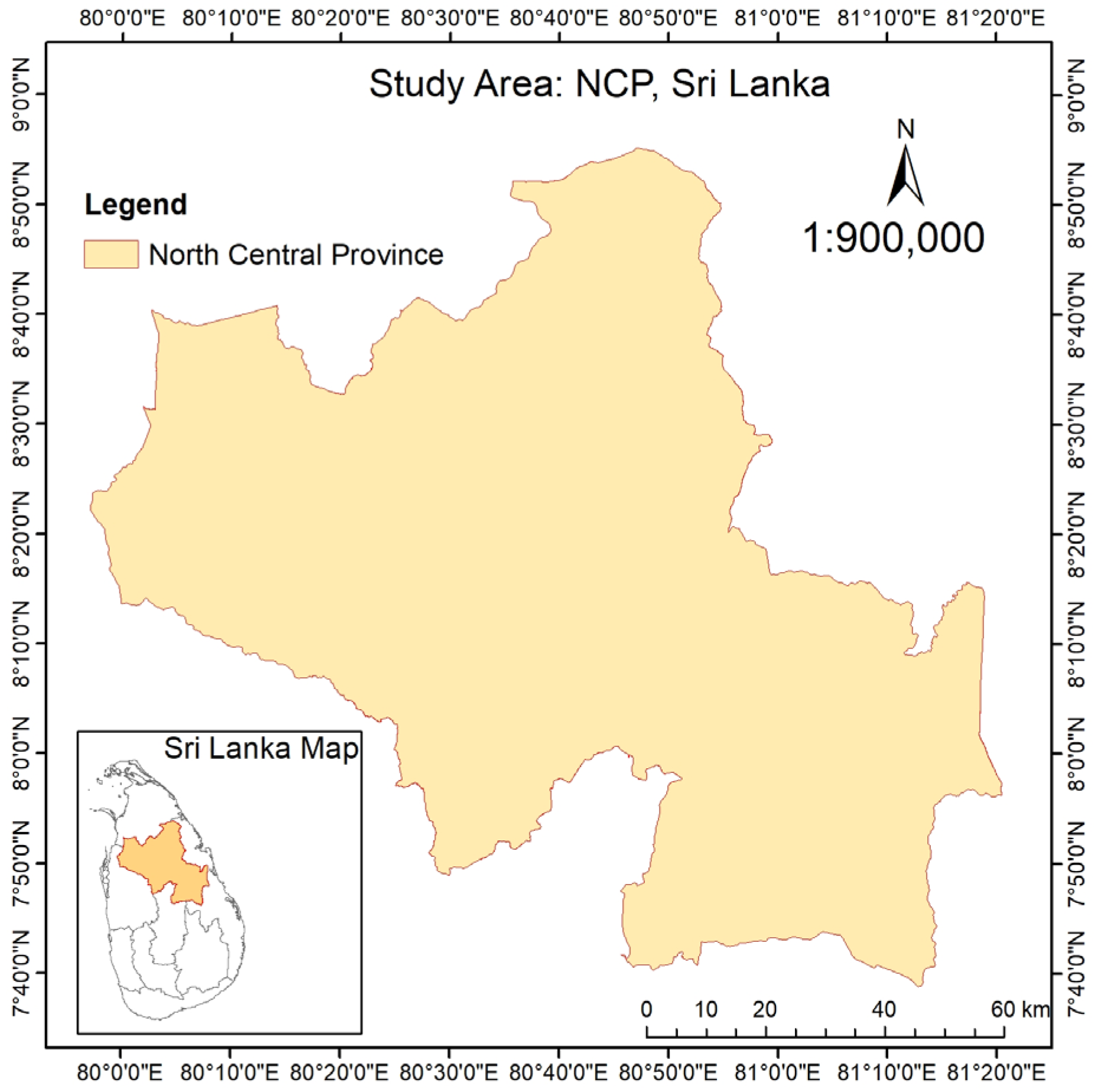
Figure 1. Study area.
Water 18 00152 g001
Figure 2. Methodology flow chart.
Water 18 00152 g002
Figure 3. Conceptual framework of study.
Water 18 00152 g003
Figure 4. Schematic diagram of this study.
Water 18 00152 g004
Figure 5. Casual loop diagram of this study.
Water 18 00152 g005
Figure 6. Water layer.
Water 18 00152 g006
Figure 7. Energy layer.
Water 18 00152 g007
Figure 8. Food layer.
Water 18 00152 g008
Figure 9. Integrated WEF layer.
Water 18 00152 g009
Figure 10. Scenario 1 output raster.
Water 18 00152 g010
Figure 11. Scenario 2 output raster.
Water 18 00152 g011
Figure 12. Scenario 3 output raster.
Water 18 00152 g012
Figure 13. Scenario 4 output raster.
Water 18 00152 g013
Figure 14. Scenario 5 output raster.
Water 18 00152 g014
Figure 15. Scenario 6 output raster.
Water 18 00152 g015
Figure 16. Scenario 7 output raster.
Water 18 00152 g016
Figure 17. Scenario 8 output raster.
Water 18 00152 g017
Figure 18. Scenario 9 output raster.
Water 18 00152 g018
Figure 19. Scenario 10 output raster.
Water 18 00152 g019
Figure 20. Scenario 11 output raster.
Water 18 00152 g020
Figure 21. Scenario 12 output raster.
Water 18 00152 g021
Table 1. Data collection.
Data TypeDerived DataSourceSpatial ResolutionTemporal Resolution
Landsat 8/9 satellite dataNDVI, NDWI, SMIUSGS Explorer, Reston, VA, USA
https://earthexplorer.usgs.gov (accessed on 17 April 2025)
30 m2020–2023
Acquisition was aligned with the phonological stages of rice to capture peak vegetation periods, from July to August for the Yala season and from January to February for the Maha season
Climate dataRainfall, solar radiation, wind speedWorldClim 2.1 dataset, University of California, Berkeley, CA, USA
https://www.worldclim.org
(accessed on 28 April 2025)
1 km2Monthly average data from 1970 to 2000 [28] (Fick and Hijamans, 2017)
Soil organic carbonSOC stock data
(0–30 cm depth)
Global Soil Organic Carbon Map (GSOCmap v2.0(2017)
http://54.229.242.119/GSOCmap/ [29] (FAO (2017) (accessed on 29 April 2025)
1 km2-
Soil typeSoil types of NCPSoils of Sri Lanka1:50,0002005 update [30,31] (Mapa et al., 2006; Hyun et al., 2015)
Electricity availabilityProximity to national gridCeylon Electricity Board Statistical Digest 20211:2,000,0002021
Land useLand use classificationLand Use Policy Planning Department (LUPPD), Sri Lanka1:50,0002018
Table 2. Classification levels and data ranges of parameters for rice paddy food layer.
Parameter
Value
Classification MethodVery High
5
High
4
Moderate
3
Low
2
Very Low
1
NDVIJenks Natural Breaks0.3497–0.53550.2983–0.34970.2372–0.29830.1199–0.2372(−0.0902)–0.1199
SOC
(Mg/ha)
Jenks Natural Breaks63–8158–6353–580–530
Soil TypeLiterature-basedAlfisolsUltisolsEntisolsLithic subgroupsErosional remnants, Rock Knob Plains
Land UseLiterature-basedAgricultural landsHome gardens, scrublandForestsWater bodiesBuilt-up
Notes: Refs. [40,41,42,43,44,45,46]. Sources: Al-Hanbali et al., 2021; Aginthini et al., 2023; Das, 2024; Malavipathirana, 2024; Mandal and Saha, 2020; Palihakkara et al. 2025; Perera et al., 2021.
Table 3. Classification levels and data ranges of parameters for rice paddy water layer.
Parameter
Value
Very High
5
High
4
Moderate
3
Low
2
Very Low
1
Rainfall
(mm)
140–168129–140118–129105–11889–105
SMI0.1587–
0.3172
0.1151–
0.1587
0.0691–
0.1152
0.02274–0.069194−0.270616–0.023274
NDWI−0.1070–
0.0943
−0.2289–
−0.1070
−0.2885–
−0.2289
−0.330844–−0.28857−0.542214–0.330844
Note: Classification type: Jenks Natural Breaks.
Table 4. Classification levels and data ranges of parameters for rice paddy energy layer.
Parameter
Value
Very High
5
High
4
Moderate
3
Low
2
Very Low
1
Proximity to national electricity grid (m)0–0.060.06–0.120.12–0.180.18–0.230.23–0.30
Solar radiation (kJ/m2/day)19,748–20,09320,093–20,28920,289–20,45620,456–20,62120,621–20,840
Wind speed (ms−1)1.58–1.821.82–1.971.97–2.112.11–2.282.28–2.64
Note: Refs. [49,50,51] (Chen et al., 2013; Li et al., 2024; Haile & Abebe, 2022).
Table 5. Scenario modeling.
Model Representation
Scenario 1: WEF interaction in the Study Area
High Food + High Water + High Energy: Optimal Resource Zone
Scenario_HFHWHE = Con (((“Food_Class” ≥ 3) & (“Water_Class” ≥ 3) & (“Energy_Class” ≥ 3)), 1, 0)
“Food_Class” ≥ 3 ➔ selects high-food-productivity areas
“Water_Class” ≥ 3 ➔ selects high-water-availability areas
“Energy_Class” ≥ 3 ➔ selects high-energy-potential areas
1 ➔ where all three conditions are true
0 ➔ elsewhere
Scenario 2: High Production Potential: High Food
Scenario_HF = Con (“Food_Class” ≥ 3, 1, 0)
“Food_Class” ≥ 3 ➔ high food availability
1 ➔ where conditions are true
0 ➔ elsewhere
Scenario 3: High Water
Scenario_HW = Con (“Water_Class” ≥ 3, 1, 0)
“Water_Class” ≥ 3 ➔ high water availability
1 ➔ where conditions are true
0 ➔ elsewhere
Scenario 4: High Energy
Scenario_HE = Con (“Energy_Class” ≥ 3, 1, 0)
“Energy_Class” ≥ 3 ➔ high energy availability
1 ➔ where conditions are true
0 ➔ elsewhere
Scenario 5: High SOC
Scenario_HC = Con (“SOC_Class” ≥ 3, 1, 0)
“SOC_Class” ≥ 3 ➔ high SOC availability
1 ➔ where conditions are true
0 ➔ elsewhere
Scenario 6: Low Food + Low SOC + Low Water (Critical Vulnerability Zone)
Scenario_LFLCLW = Con ((“Food_Class” ≤ 3) & (“SOC_Class” ≤ 3) & (“Water_Class” ≤ 3), 1, 0)
“Food_Class” ≤ 3 ➔ low food productivity
“SOC_Class” ≤ 3 ➔ low SOC availability
“Water_Class” ≤ 3 ➔ low water availability
1 ➔ where all three conditions are true
0 ➔ elsewhere
Scenario 7: High energy + Low Food + Low Water (Energy-driven Zone)
Scenario_HELFLW = Con (((“Energy_Class” ≥ 3) & (“Food_Class” ≤ 3) & (“Water_Class” ≤ 3)), 1, 0)
“Energy_Class” ≥ 3 ➔ high energy availability
“Food_Class” ≤ 3 ➔ low food productivity
“Water_Class” ≤ 3 ➔ low water availability
1 ➔ where all three conditions are true
0 ➔ elsewhere
Scenario 8: Low Food + High Water + Low Energy (Energy-Constraint Zone)
Scenario_LFHWLE = Con (((“Food_Class” ≤ 3) & (“Water_Class” ≥ 3) & (“Energy_Class” ≤ 3)), 1, 0)
“Food_Class” ≤ 3 ➔ low food productivity
“Water_Class” ≥ 3 ➔ high water availability
“Energy_Class” ≤ 3 ➔ low energy availability
1 ➔ where all three conditions are true
0 ➔ elsewhere
Scenario 9: High Food + Low Water + High Energy (Adaptive Agricultural Zone)
Scenario_HFLWHE = Con (((“Food_Class” ≥ 3) & (“Water_Class” ≤ 3) & (“Energy_Class” ≥ 3)), 1, 0)
“Food_Class” ≥ 3 ➔ high food productivity
“Water_Class” ≤ 3 ➔ low water availability
“Energy_Class” ≥ 3 ➔ high energy availability
1 ➔ where all three conditions are true
0 ➔ elsewhere
Scenario 10: High Food + Low Water
Scenario_HFLW = Con ((“Food_Class” ≥ 3) & (“Water_Class” ≤ 3), 1, 0)
“Food_Class” ≥ 3 ➔ high food productivity
“Water_Class” ≤ 3 ➔ low water availability
1 ➔ where all two conditions are true
0 ➔ elsewhere
Scenario 11: Low Food + Low SOC
Scenario_LFLC = Con ((“Food_Class” ≤ 3) & (“SOC_Class” ≤ 3), 1, 0)
“Food_Class” ≤ 3 ➔ low food availability
“SOC_Class” ≤ 3 ➔ low SOC availability
1 ➔ where all two conditions are true
0 ➔ elsewhere
Scenario 12: High Solar + High Wind (Renewable Energy Potential)
Scenario_HSoLWi = Con ((“Solar_Class” ≥ 3) & (“Wind_Class” ≥ 3), 1, 0)
“Solar_Class” ≥ 3 ➔ high solar energy
“Wind_Class” ≥ 3 ➔ high wind energy
1 ➔ where all two conditions are true
0 ➔ elsewhere
Table 6. Summary of validation statistics for water layer.
StatisticLayer 1 (Water Hotspot)Layer 2 (Water Availability Scenario)
Minimum (MIN)0.00000.0000
Maximum (MAX)1.00001.0000
Mean0.45230.5398
Standard Deviation (SD)0.49770.4964
Covariance Matrix
Layer12
10.121560.08979
20.089790.12156
Correlation Matrix
Layer12
11.000000.73717
20.737171.00000
Table 7. Summary of validation statistics for energy layer.
StatisticLayer 1 (Energy Hotspot)Layer 2 (Energy Availability Scenario)
Minimum (MIN)0.00000.0000
Maximum (MAX)1.00001.0000
Mean0.68180.4316
Standard Deviation (SD)0.46580.4958
Covariance Matrix
Layer12
10.104720.06498
20.064980.10472
Correlation Matrix
Layer12
11.000000.58161
20.581611.00000
Table 8. Summary of validation statistics for food layer.
StatisticLayer 1 (Food Hotspot)Layer 2 (Food Availability Scenario)
Minimum (MIN)0.00000.0000
Maximum (MAX)1.00001.0000
Mean0.57830.9398
Standard Deviation (SD)0.49380.2378
Covariance Matrix
Layer12
10.119600.01573
20.015730.02775
Correlation Matrix
Layer12
11.000000.27304
20.273041.00000
Table 9. Correlation validation table.
Pair (Layers)r (Pearson)n (Valid Pixels)p-ValueInterpretation
Water Hotspot vs. Water Scenario 0.7371710,542<0.001Indicates a strong positive correlation between hotspot zones and scenarios
Energy Hotspot vs. Energy Scenario0.581619863<0.001Indicates a moderate positive correlation between hotspot zones and scenarios
Food Hotspot vs. Food Scenario0.2730412,000<0.001Indicates a mild positive correlation between hotspot zones and scenarios
Disclaimer/Publisher’s Note: The statements, opinions and data contained in all publications are solely those of the individual author(s) and contributor(s) and not of MDPI and/or the editor(s). MDPI and/or the editor(s) disclaim responsibility for any injury to people or property resulting from any ideas, methods, instructions or products referred to in the content.