Explainable ML for Irrigation Water Quality Prediction in the Sedrata Aquifer, Plain (Algeria)

Abstract

Accurate assessment of irrigation water quality is essential for sustainable groundwater management in semi-arid regions. Conventional Irrigation Water Quality Index (IWQI) assessment requires multiple physicochemical measurements and manual computation of a composite index, which can be time-consuming, costly, and difficult to scale across repeated monitoring campaigns. Machine learning (ML) approaches may provide a practical surrogate for reconstructing IWQI from a reduced set of routinely measured variables. This study developed an interpretable ML framework for IWQI reconstruction in the shallow phreatic aquifer of the Sedrata Plain, northeastern Algeria. One hundred groundwater samples were collected from 25 open wells across four seasonal campaigns (February 2023–May 2024). IWQI was calculated from EC, Na⁺, Cl⁻, HCO₃⁻, and SAR using the weighted aggregation approach of Meireles et al. Six ML algorithms were assessed using nested Recursive Feature Elimination with Cross-Validation (RFECV) within a Leave-One-Campaign-Out (LOCO) validation framework, with predictive performance evaluated using R², RMSE, and MAE. IWQI values ranged from 28.72 to 76.28, with 8%, 56%, 28%, and 8% classified as low, moderate, high, and severe restriction, respectively. Extreme Gradient Boosting (XGBoost) achieved the highest LOCO performance (R² = 0.732 ± 0.109; RMSE = 5.075 ± 1.403 IWQI units), compared with Multiple Linear Regression (MLR) (R² = 0.563 ± 0.304). SHapley Additive exPlanations (SHAP) identified Cl⁻, EC, and SAR as the dominant predictors. The findings demonstrate the potential of an interpretable ML framework for grouped-validation IWQI reconstruction from routinely measured variables, supporting efficient irrigation-water quality screening. External validation is required before wider application.

1. Introduction

Groundwater is a vital source of freshwater for agricultural irrigation in arid and semi-arid regions where surface-water availability is limited and highly variable [1]. In these environments, groundwater quality is affected by lithological interactions, evaporative concentration, seasonal recharge, and anthropogenic pressures such as agricultural activities and over-extraction [2,3]. Excessive salinity, sodicity, and concentrations of ions such as chloride, sodium, and bicarbonate can degrade soil structure, reduce hydraulic conductivity, and impair crop growth [4]. Consequently, reliable irrigation-water quality assessment is essential for sustainable agriculture and groundwater management. However, comprehensive physicochemical monitoring can be costly and logistically demanding in data-scarce regions such as northeastern Algeria, motivating the development of data-driven surrogate approaches that can estimate composite quality indices from routinely measured variables.

The Irrigation Water Quality Index (IWQI), proposed by Meireles et al. [5] within the framework of FAO irrigation-water guidelines [6], integrates multiple physicochemical parameters into a single score describing irrigation-water restriction. It has been widely applied in arid and semi-arid groundwater systems [7]. However, direct IWQI calculation requires a prescribed set of physicochemical inputs and empirical scoring functions. Machine-learning (ML) methods can therefore provide a surrogate approach for reconstructing computed IWQI values from measurable hydrochemical variables, including nonlinear relationships and interactions that may be difficult to represent using conventional linear models [8,9]. Tree-based ensemble methods such as Random Forest, Gradient Boosting, and Extreme Gradient Boosting (XGBoost) [3,8,9] have shown strong performance in water-quality modelling [10,11].

Model interpretability remains an important challenge because high-performing ML models may provide limited insight into how individual predictors contribute to their outputs. SHapley Additive exPlanations (SHAP) provides a unified framework for quantifying feature contributions to individual model predictions and summarising model-level feature importance [12,13]. Recent studies have increasingly combined ML and SHAP for water-quality and irrigation-water quality assessment. Hussein et al. [14] evaluated several ML algorithms for IWQI prediction and reported strong performance by XGBoost, while Gaagai et al. [15], Azlaoui et al. [11], Zegaar et al. [16], M’nassri et al. [17], Nefla et al. [18], and Panagiotou et al. [19] demonstrated the applicability of ML-based approaches to irrigation-water quality assessment in Algerian and Tunisian groundwater systems. These studies demonstrate the potential of ML and explainability methods for hydrochemical assessment; however, reported predictive performance alone does not establish generalisation to previously unseen wells or sampling campaigns.

A growing body of literature has applied ML-based approaches specifically to IWQI prediction and reconstruction across diverse hydrogeological settings. Hussein et al. [14] compared SVR, KNN, Random Forest, and XGBoost for IWQI prediction using a conventional random 80/20 train–test split, reporting R² values of 0.92–0.97 for the best-performing models, with XGBoost achieving the highest accuracy. Gaagai et al. [15] combined GIS mapping with ML-based water-quality indices for irrigation-suitability assessment in the Sahara Aquifer of the Doucen Plain, Algeria, demonstrating the feasibility of data-driven approaches in data-scarce arid environments. In Algeria, Azlaoui et al. [11] applied an XGBoost framework with SHAP interpretability to IWQI prediction in a semi-arid groundwater system, reporting test-set R² values of approximately 0.85–0.92 under random data partitioning and identifying EC and Na⁺ as dominant predictors. Zegaar et al. [16] developed interpretable ML models for irrigation sustainability in the M’sila region, Algeria, using SHAP to rank hydrochemical predictors of IWQI. In Tunisia, M’nassri et al. [17] applied a data-driven approach to IWQI estimation in a semi-arid aquifer, while Panagiotou et al. [19] proposed a generalised ML framework for cost-effective irrigation-suitability monitoring in the El Fahs aquifer using Random Forest and Gradient Boosting. Nefla et al. [18] Further integrated GIS, ML, and SHAP for irrigation-water quality assessment in a coastal Algerian groundwater system. Collectively, these studies demonstrate the potential of ML, particularly ensemble approaches, for reconstructing composite irrigation-water quality indices from measurable hydrochemical predictors and show that SHAP can provide useful model-level attribution of predicted water-quality indices. However, many of these studies rely on random train–test partitioning, which may provide optimistic estimates of generalisation when repeated observations from the same monitoring wells are distributed across training and testing subsets. To the best of our knowledge, an integrated LOCO and LOWO grouped-validation framework has not previously been reported for the Sedrata Plain phreatic aquifer.

Several methodological gaps therefore remain relevant. First, many ML-based IWQI studies use random train–test partitioning even when repeated observations originate from the same wells, potentially allowing well-specific information to occur in both training and testing subsets and thereby producing optimistic estimates of generalisation [20,21]. Second, because IWQI is a deterministic composite index calculated from prescribed physicochemical inputs, ML-based IWQI modelling represents surrogate reconstruction of a mathematical transformation rather than prediction of an independent environmental outcome. This distinction is important when interpreting both predictive performance and SHAP feature attributions. Third, to the best of our knowledge, an integrated validation framework combining temporally grouped Leave-One-Campaign-Out (LOCO) and well-level Leave-One-Well-Out (LOWO) validation with SHAP-based interpretation has not been reported for the Sedrata Plain phreatic aquifer.

Accordingly, this study develops an ML framework designed to minimise information leakage in the surrogate reconstruction of IWQI for the Sedrata Plain phreatic aquifer, northeastern Algeria. The framework makes four methodological contributions: (i) nested LOCO cross-validation is used as the primary campaign-level validation strategy, with predictor selection and hyperparameter optimisation performed exclusively within each training partition; (ii) LOWO validation is used as a complementary assessment of well-level generalisation to previously unseen wells; (iii) the deterministic IWQI calculation and a pre-specified Multiple Linear Regression (MLR) model are used as reference baselines, while SHAP values are interpreted strictly as measures of model-level feature reliance rather than causal hydrogeochemical effects; and (iv) Recursive Feature Elimination with Cross-Validation (RFECV) is nested within the outer LOCO training folds to prevent information leakage during predictor selection. The specific objectives are to characterise groundwater irrigation quality in the Sedrata Plain, evaluate the performance of nonlinear and linear ML models for IWQI surrogate reconstruction under grouped validation, assess the consistency of model performance across sampling campaigns and wells, and interpret model-level predictor reliance using SHAP.

2. Materials and Methods

2.1. Study Site and Groundwater Sampling

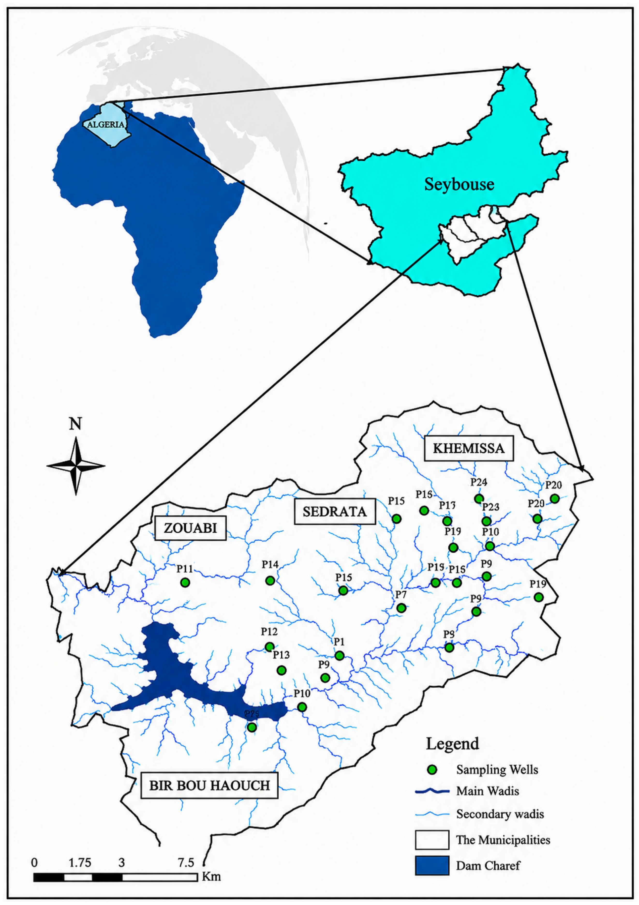
The study was conducted in the Wadi Cherf/Sedrata basin, which forms part of the Seybouse watershed in northeastern Algeria. Geographically, the study area is located at approximately 36°07′42″ N latitude and 7°31′53″ E longitude, at an elevation ranging from approximately 804 to 811 m above sea level. Administratively, the study area belongs to the municipality of Sedrata, one of the largest municipalities in Souk Ahras Province [22]. It is located approximately 56 km southwest of the provincial capital, Souk Ahras, and about 85 km from the Mediterranean Sea (Figure 1).

The Sedrata area covers approximately 355 km² and has a population of 80,197 inhabitants [23]. The region has considerable agricultural potential, owing mainly to its predominantly flat geomorphological setting, which favors extensive cultivation of cereals and fodder crops, as well as sheep farming. Agriculture constitutes the main economic activity, whereas the industrial sector remains relatively limited and is represented by several industrial units distributed throughout the municipality [24].

Hydrogeologically, the groundwater investigated in this study corresponds to the shallow phreatic aquifer of the Sedrata Plain. The aquifer is hosted mainly within a Mio-Plio-Quaternary sedimentary cover composed of sandy clays, sands, gravels, sandstones, and calcareous materials. Available hydrogeological information indicates a mean transmissivity of about 3 × 10⁻⁴ m²/s and a mean permeability of approximately 1.2 × 10⁻⁵ m/s, indicating the capacity of the aquifer materials to transmit groundwater [22]. The aquifer is exploited locally through boreholes, open wells, and springs, reflecting its importance as a groundwater resource.

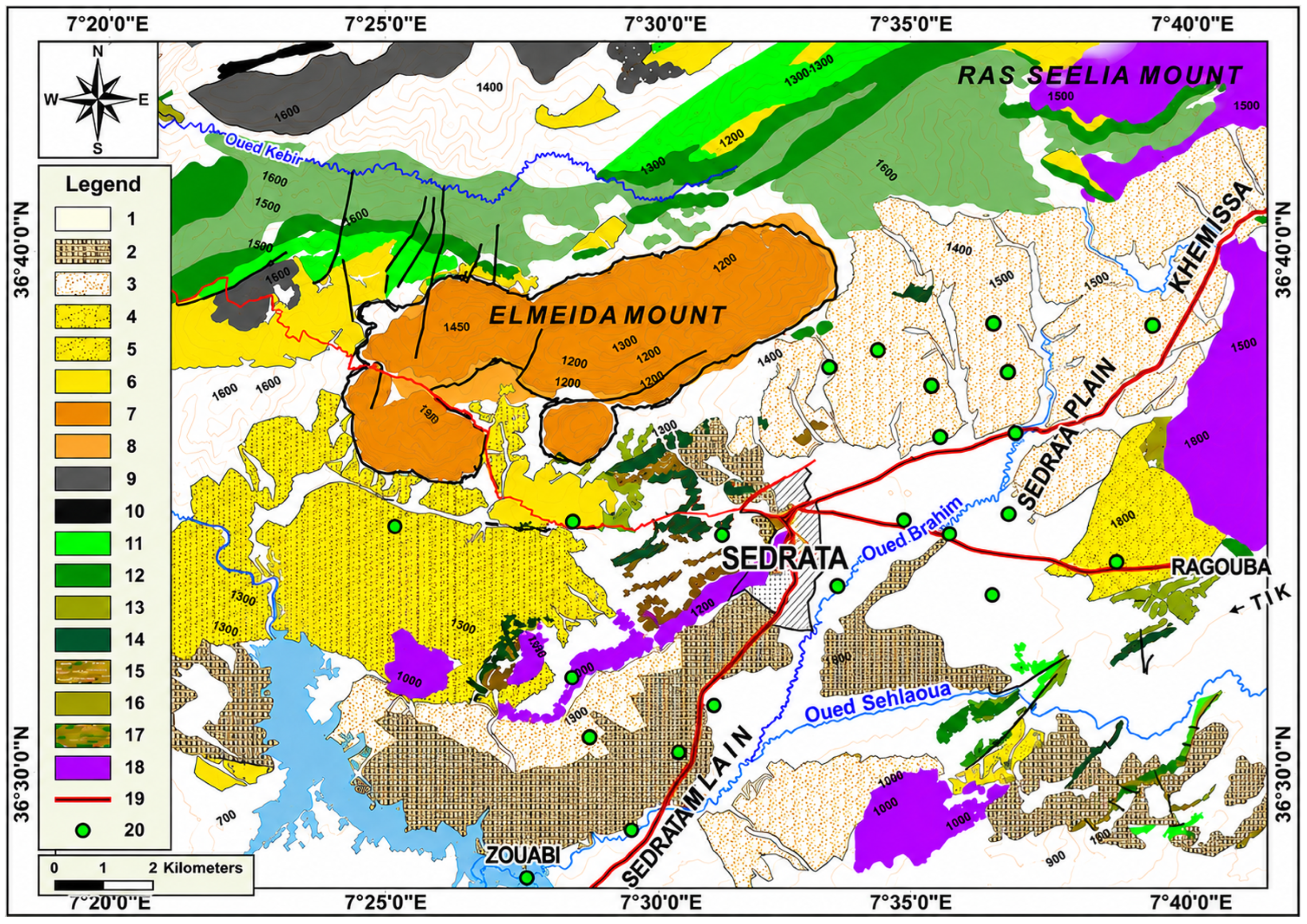
Based on geological studies of the Sedrata region and surrounding areas [25,26,27,28,29,30], the regional geological framework comprises autochthonous and parautochthonous formations, together with allochthonous Tellian and Numidian units, unconformably overlain by a post-nappe Mio-Plio-Quaternary sedimentary cover. The latter consists mainly of Pliocene conglomerates and red clays, Villafranchian calcareous crusts, and Quaternary fluvial and colluvial deposits, which form the principal shallow hydrogeological unit of the plain. These deposits host a shallow phreatic aquifer extending over approximately 190 km², with permeable horizons mainly consisting of sands and gravels interbedded with sandy-clayey materials. Groundwater recharge is considered to occur mainly through effective precipitation, while groundwater circulation is influenced by the heterogeneous lithological and sedimentary characteristics of the aquifer. At greater depth, the Maastrichtian carbonate formations of the Sellaoua and North Aurès units constitute a fractured aquifer and represent an additional groundwater reservoir within the regional hydrogeological system. The heterogeneous geological framework, including carbonate, marl, clay, sandstone, and evaporitic formations, provides a plausible geological context for the spatial variability of groundwater mineralization observed in the study area (Figure 2).

Groundwater sampling was conducted from 25 open wells distributed across the Sedrata plain. The sampled wells had depths ranging from approximately 3 to 25 m and therefore primarily represent the shallow phreatic groundwater system investigated in this study. Four sampling campaigns were conducted in February 2023, May 2023, December 2023, and May 2024, yielding 100 groundwater samples. The sampling network was designed to provide broad and relatively homogeneous spatial coverage of the study area and to capture spatial and temporal variations in groundwater hydrochemistry across the four sampling periods.

Groundwater samples were collected in 1.5-L high-density polyethylene (HDPE) bottles. Each bottle was labeled with the corresponding well identification, sampling date, and well depth. Samples were preserved at 4 °C and transported to the laboratory for analysis in accordance with the recommendations of the American Public Health Association [31]. All physicochemical analyses were performed at the laboratory of the Algerian Water Company (ADE). pH, electrical conductivity (EC), and temperature (T) were measured in situ using a WTW multiparameter meter (WTW, Weilheim, Germany). Turbidity was measured using a calibrated turbidity meter (HACH 2100N, Hach, Loveland, CO, USA), while dissolved oxygen (DO) was determined in situ using a pre-calibrated DO meter following standard procedures. The ion balance (IB) method was applied to verify the accuracy of the chemical analyses for each sample, with all samples falling within the acceptable limit of ±10% [32,33].

Two additional hydrochemical indices were calculated from the laboratory measurements using Equations (1) and (2) given below and were included as candidate predictor variables.

Sodium Adsorption Ratio

$$SAR={\displaystyle \frac{\left[{Na}^{+}\right]}{\sqrt{\frac{\left[{Ca}^{2+}\right] + \left[{Mg}^{2+}\right]}{2}}}}$$

(1)

where Na⁺, Ca²⁺, and Mg²⁺ are the concentrations of sodium, calcium, and magnesium ions, respectively, expressed in milliequivalents per litre (meq/L). SAR was used to evaluate the sodicity hazard of the irrigation water [34].

Total Hardness (TH):

$$\mathrm{T}\mathrm{H}\left(\mathrm{m}\mathrm{g}/\mathrm{L} \mathrm{a}\mathrm{s} {\mathrm{C}\mathrm{a}\mathrm{C}\mathrm{O}}_3\right)=\left(2.497\times {Ca}^{2+}\right)+(4.118\times {Mg}^{2+})$$

(2)

where Ca²⁺ and Mg²⁺ are expressed in mg/L, and the coefficients 2.497 and 4.118 are the CaCO₃ equivalent conversion factors for calcium and magnesium, respectively. TH is expressed in mg/L as CaCO₃ [31]. Both SAR and TH are derived variables, not directly measured, and their calculation is documented in the dataset and confirmed by cross-checking against the original ion concentrations.

Data quality and preprocessing: The complete analytical dataset (n = 100, 12 measured parameters plus 2 derived indices) was inspected for missing values and anomalous entries prior to modelling; no missing values were identified. No formal outlier-removal procedure was applied: observations with extreme values in parameters such as EC, K⁺, Ca²⁺ or turbidity were retained because they represent genuine groundwater conditions and carry environmentally meaningful information, and removing them would artificially reduce the representativeness of the dataset. The high skewness and kurtosis values reported for several parameters (e.g., Ca²⁺: skewness = 2.50; K⁺: skewness = 4.49) confirm the presence of high-concentration observations, retained as scientifically valid data points.

Scaling: All candidate predictor variables were normalized using Min–Max scaling prior to feature selection and model fitting, according to the equation given below (Equation (3)) [35]:

$${\mathrm{x}}^{\prime }={\displaystyle \frac{\mathrm{X}-X_{min}}{X_{max}-X_{min}}}$$

(3)

where ($\mathrm{X}$) is the original value, (x′) is the scaled value in the range [0, 1], and ($X_{min}$) and ($X_{max}$) are the minimum and maximum values of ($\mathrm{X}$), respectively. Consistent with the nested validation framework, the scaling parameters were estimated exclusively from the training data within each cross-validation fold and subsequently applied to the corresponding validation observations, thereby preventing information leakage from the validation data into the scaling procedure [36].

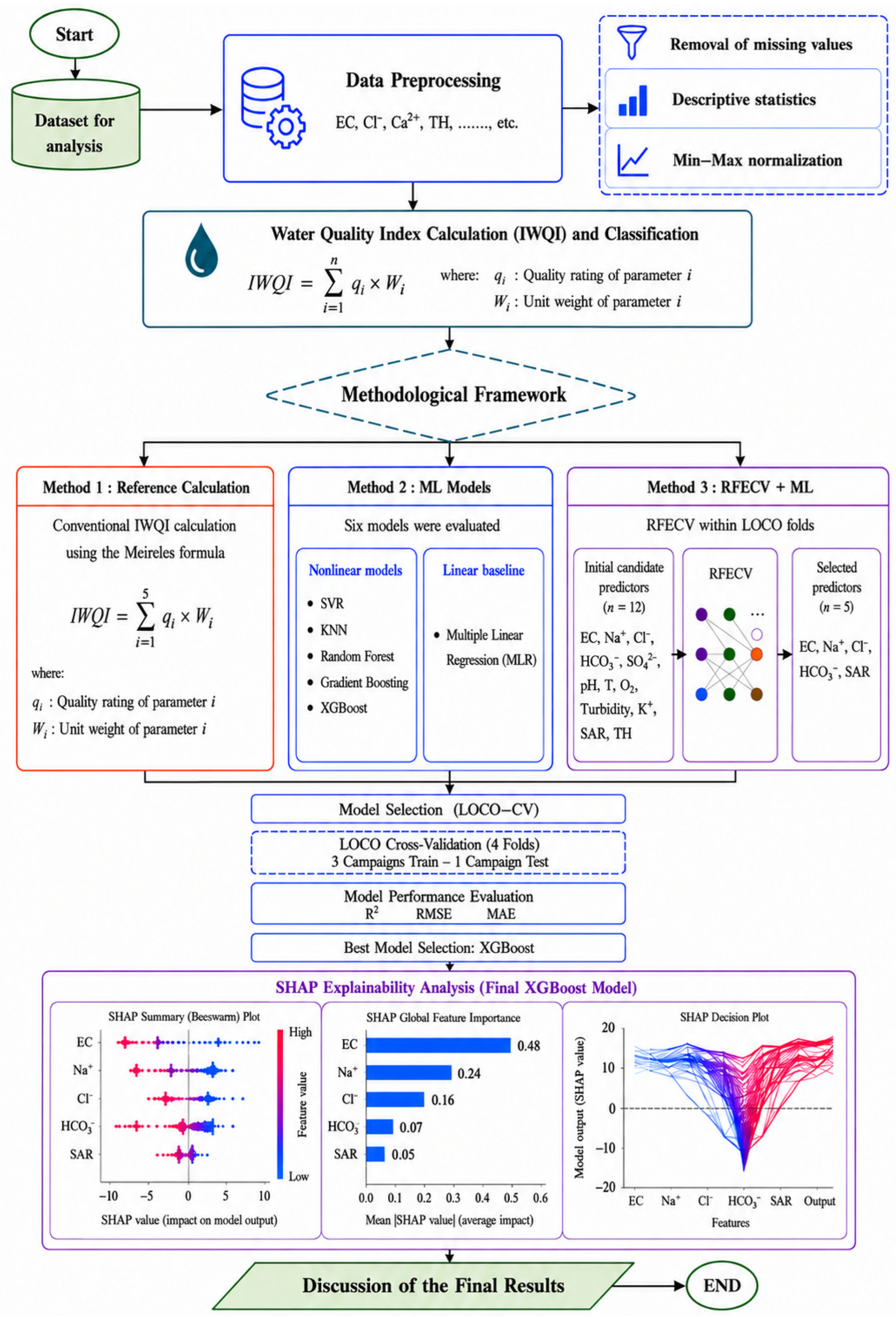
An integrated methodological framework was developed to provide an overview of the analytical strategy adopted in this study (Figure 3). The framework combines IWQI assessment, machine-learning modelling, feature selection using RFECV within the LOCO-CV scheme, and SHAP-based explainability. This workflow enables the systematic assessment, prediction, and interpretation of groundwater quality.

2.2. Irrigation Water Quality Index Computation

The Irrigation Water Quality Index (IWQI) was used to provide an integrated assessment of groundwater suitability for irrigation. The index was calculated using the weighted aggregation approach of Meireles et al. [5]. In the present study, IWQI was calculated from five parameters: electrical conductivity (EC), sodium (Na⁺), bicarbonate (HCO₃⁻), chloride (Cl⁻), and sodium adsorption ratio (SAR). These parameters are direct components of the IWQI formulation and were subsequently used as the target-defining predictors for the machine-learning models.

For each parameter, a quality rating (q_i) was calculated from the corresponding concentration bands and threshold values given in

Table 1. Concentration bands and corresponding q_i ranges for IWQI computation [37].

qi Range	EC (dS/m)	Na+ (meq/L)	Cl− (meq/L)	HCO3− (meq/L)	SAR (Dimensionless 1/2)
85–100	0.20 ≤ EC < 0.75	2 ≤ Na < 3	1 ≤ Cl < 4	1 ≤ HCO3 < 1.5	2 ≤ SAR < 3
60–85	0.75 ≤ EC < 1.50	3 ≤ Na < 6	4 ≤ Cl < 7	1.5 ≤ HCO3 < 4.5	3 ≤ SAR < 6
35–60	1.50 ≤ EC < 3.00	6 ≤ Na < 9	7 ≤ Cl < 10	4.5 ≤ HCO3 < 8.5	6 ≤ SAR < 12
0–35	EC < 0.20 or EC ≥ 3.00	Na < 2 or Na ≥ 9	Cl < 1 or Cl ≥ 10	HCO3 < 1 or ≥8.5	SAR < 2 or SAR ≥ 12

, using [5]:

$$q_i=q_{max}-\left({\displaystyle \frac{\left[\left(x_{ij}-x_{inf}\right)q_{imap}\right]}{x_{amp}}}\right)$$

(4)

where ($q_i$) is the quality rating assigned to the (i)-th parameter, (q_max) represents the maximum allowable quality rating, and (x_i) denotes the observed concentration or value of the parameter. The term (x_inf) refers to the lower boundary of the relevant parameter class, (q_iamp) represents the amplitude of the corresponding quality-rating interval, and (x_amp) denotes the amplitude of the respective parameter class.

The overall IWQI was subsequently obtained using a weighted additive aggregation approach [5]:

$$\mathrm{I}\mathrm{W}\mathrm{Q}\mathrm{I}={\sum }_{\mathrm{i}=1}^{\mathrm{n}}\left({\mathrm{q}}_{\mathrm{i}}\times {\mathrm{W}}_{\mathrm{i}}\right)$$

(5)

where ${\mathrm{q}}_{\mathrm{i}}$ is the quality score of parameter i, calculated from the measured concentration x_ij using the linear interpolation equation (Equation (4)) within the applicable concentration band defined in Table 1, and W_i is its empirical weighting coefficient (

Table 2. Empirical weighting coefficients for IWQI computation [37].

Parameter	Wi
EC	0.211
Na+	0.204
Cl−	0.194
HCO3−	0.202
SAR	0.189
Total	1.000

).

The resulting IWQI values were classified into five restriction categories: no restriction (NR: 85–100), low restriction (LR: 70–85), moderate restriction (MR: 55–70), high restriction (HR: 40–55), and severe restriction (SR: 0–40). IWQI values were calculated for all 100 groundwater samples before model training and used as the target variable in the machine-learning analyses [5].

2.3. Feature Selection

2.3.1. Correlation and Multicollinearity Analysis

Pearson’s product–moment correlation analysis was performed on the complete dataset (n = 100) to describe the linear associations between the candidate predictors and the computed IWQI. The correlation coefficient (r) and corresponding p-value were evaluated, with correlation strength interpreted according to Dancey and Reidy [38]. Pearson correlation was used solely for descriptive purposes and was not used as a predictor-selection criterion. Because IWQI is a deterministic function of several physicochemical variables, correlations with EC, Na⁺, Cl⁻, HCO₃⁻, and SAR were interpreted as reflecting, at least partly, the mathematical construction of the index rather than independent predictive or causal relationships.

Multicollinearity was assessed using the variance inflation factor (VIF):

$${VIF}_j={\displaystyle \frac{1}{1-R_j^2}}$$

(6)

where $R_j^2$ is the coefficient of determination obtained by regressing predictor j against all other candidate predictors. A VIF value of 1 indicates no linear dependence, whereas higher values indicate increasing multicollinearity. A threshold of VIF > 10 was used to indicate severe multicollinearity [39,40].

VIF assessment was performed exclusively within the outer training partition of each LOCO fold, thereby preventing the held-out campaign from contributing to predictor screening. Where perfect collinearity occurred between a derived index and its constituent variables, the constituent variables were excluded, and the derived index was retained; specifically, Ca²⁺ and Mg²⁺ were excluded because of their perfect collinearity with TH (VIF = ∞), while TH was retained as the aggregate hardness indicator. Following this step, 12 candidate predictors were passed to RFECV.

2.3.2. Recursive Feature Elimination with Cross-Validation (RFECV)

Recursive Feature Elimination with Cross-Validation (RFECV) was used to identify a parsimonious predictor subset for IWQI reconstruction [38,39]. A Random Forest (RF) regressor was used as the base estimator because it can capture nonlinear relationships and interactions and provides feature-importance estimates [40,41]. RFECV was implemented using scikit-learn [42], with the least important predictor recursively removed and model performance evaluated using inner five-fold cross-validation. The coefficient of determination (R²) was used as the scoring criterion, and the subset yielding the highest mean cross-validated R² was selected.

To prevent information leakage, RFECV was performed independently within each outer LOCO training partition (n = 75), with the corresponding held-out campaign excluded from feature selection. The selected predictors were then used for subsequent hyperparameter optimisation and model fitting within the same training partition.

2.4. Machine Learning Models

Six machine-learning approaches were evaluated for IWQI reconstruction: Support Vector Regression (SVR), K-Nearest Neighbours (KNN), Random Forest (RF), Gradient Boosting (GB), Extreme Gradient Boosting (XGBoost), and Multiple Linear Regression (MLR). These models represent complementary learning paradigms, including kernel-based, instance-based, linear, and tree-based ensemble methods [16,43].

Within each outer LOCO fold, candidate predictors were first subjected to VIF-based multicollinearity assessment and RFECV using the training data only. The selected predictors were then used for model fitting and hyperparameter optimisation. Min–Max scaling was applied consistently within the modelling pipeline, with transformation parameters estimated exclusively from the corresponding training partition and applied unchanged to held-out observations. Although scaling is particularly important for distance- and kernel-based algorithms such as KNN and SVR, tree-based models are largely insensitive to feature magnitude [8,9]. The same training-derived preprocessing framework was maintained across validation folds to prevent information leakage [42].

2.4.1. Nested Modelling Procedure

A nested modelling framework was implemented within the outer Leave-One-Campaign-Out (LOCO) validation scheme to separate model development from final evaluation and minimise optimistic performance estimates [35,44]. For each outer fold, one complete sampling campaign was held out as the test set, while all model-development procedures were performed exclusively on the remaining training observations.

The within-fold workflow consisted of: (1) VIF assessment of the candidate predictors using the outer training data; (2) RFECV using a Random Forest regressor and inner five-fold cross-validation with R² as the scoring criterion; (3) retention of the RFECV-selected predictors; (4) estimation of Min–Max scaling parameters from the outer training partition and application of the same transformation to the held-out campaign; (5) hyperparameter optimisation using GridSearchCV with inner three-fold cross-validation and R² as the optimisation criterion; (6) refitting of each model on the complete outer training partition using the selected predictors and optimal hyperparameters; and (7) prediction and evaluation on the held-out campaign using R², RMSE, and MAE.

Thus, the held-out campaign remained independent of preprocessing, feature selection, and hyperparameter optimisation. The resulting out-of-fold predictions constituted the primary basis for assessing model generalisation. A fixed random state of 0 was used for stochastic algorithms (RF, GB, and XGBoost), whereas the secondary random 80/20 reference split used random state = 42.

2.4.2. Hyperparameter Optimisation

Hyperparameter optimisation was performed using GridSearchCV implemented in scikit-learn [42]. Within each outer LOCO training fold, predefined parameter combinations were evaluated using three-fold internal cross-validation and R² as the optimisation criterion. The configuration with the highest mean cross-validated R² was selected, and the model was subsequently refitted using the complete training partition.

The predefined parameter grids were:

KNN: n_neighbors = {3, 5, 7, 9}; weights = {uniform, distance}; metric = {euclidean, manhattan}.

SVR: RBF kernel; C = {1, 10, 100}; ε = {0.1, 0.2, 0.5}; γ = {auto, scale}.

Random Forest: n_estimators = {100, 200}; max_depth = {10, 20, None}; max_features = {sqrt}; min_samples_leaf = {1, 2}.

Gradient Boosting: n_estimators = {100, 200}; learning_rate = {0.05, 0.1}; max_depth = {3, 5}.

XGBoost: n_estimators = {100, 200}; learning_rate = {0.05, 0.1}; max_depth = {4, 6}; subsample = 0.8; colsample_bytree = 0.8.

MLR was used as a linear baseline and did not require hyperparameter optimisation. The same outer training and held-out partitions were maintained for comparison with the nonlinear models.

2.4.3. Software and Computational Environment

All data preprocessing, statistical analyses, and machine-learning procedures were performed using Python 3.7.3. The Scikit-learn package (version 0.20.2) was used for data preprocessing, feature selection using RFECV, hyperparameter optimization using GridSearchCV, and implementation and evaluation of the machine-learning models.

2.5. Baseline Model and Grouped Validation

Multiple Linear Regression (MLR) was included as a transparent linear baseline for comparison with the nonlinear machine-learning models [45]. MLR used the five variables directly incorporated into the IWQI formulation: EC, Na⁺, Cl⁻, HCO₃⁻, and SAR [16]. These predictors were specified a priori from the mathematical structure of the IWQI and were not selected using Pearson correlation or RFECV; MLR was therefore treated as a predefined linear reconstruction model.

Min–Max scaling was applied to the MLR predictors within each outer training partition using training-derived parameters only, consistent with the preprocessing pipeline described in Section 2.4. The deterministic IWQI calculation was treated as a definitional reference rather than a competing machine-learning model because IWQI is mathematically determined by its prescribed scoring and weighting functions. Model performance was therefore evaluated according to the ability of the machine-learning approaches to reconstruct this predefined index from measured hydrochemical predictors.

2.5.1. Leave-One-Campaign-Out (LOCO) Validation

The primary validation strategy was Leave-One-Campaign-Out (LOCO) cross-validation, designed to assess model transferability to an unseen sampling campaign [46]. Four outer folds were constructed, with one complete campaign (25 observations) held out in each fold and the remaining three campaigns (75 observations) used for model development:

February 2023;

May 2023;

December 2023; and

May 2024.

Within each outer fold, all preprocessing, VIF assessment, RFECV, hyperparameter optimisation, and model fitting were performed exclusively using the training observations. The held-out campaign was used only for final prediction and performance assessment. R², RMSE, and MAE were calculated from the held-out observations. Because only four campaigns were available, LOCO was interpreted as an assessment of transferability across the observed campaigns rather than evidence of general temporal performance beyond the study period.

2.5.2. Leave-One-Well-Out (LOWO) Cross-Validation Procedure

As a secondary grouped validation, Leave-One-Well-Out (LOWO) cross-validation was performed using the monitoring-well identifier as the grouping variable [47]. Twenty-five folds were constructed, with all four observations from one well held out in each fold and the remaining 24 wells used for model development. Thus, observations from the same well never occurred simultaneously in the training and test partitions.

Within each LOWO fold, preprocessing, VIF-based multicollinearity assessment, RFECV feature selection, hyperparameter optimisation, and model fitting were performed exclusively using the training wells. The held-out well was used only for final prediction and evaluation. Because each test fold contained only four observations, RMSE and MAE were used as the primary fold-level error metrics, whereas fold-level R² was interpreted cautiously [48].

2.5.3. Random 80/20 Split as a Secondary Reference

A conventional random 80/20 train–test split (random state = 42) was retained only as a secondary reference for comparison with studies using random data partitioning. Model development was performed on the training subset, while the test subset was reserved for final evaluation. Because repeated observations from the same monitoring wells may occur in both subsets, random splitting can provide optimistic estimates of generalisation. It was therefore not used as the primary validation strategy; model generalisation was assessed principally using LOCO, supplemented by LOWO validation.

2.6. Model Evaluation

Model performance was assessed using three complementary metrics: Root Mean Squared Error (RMSE), Mean Absolute Error (MAE), and the coefficient of determination (R²). These metrics were selected because they provide complementary information on predictive accuracy and are widely used in water-quality and IWQI modelling [15,20,34,41,42,43,44,45,46,47,48,49]; their joint use is recommended by Willmott and Matsuura [50] and supported by Chai and Draxler [46], who demonstrated the complementary diagnostic properties of MAE and RMSE in assessing model performance [51].

The RMSE is calculated as follows:

$$\mathrm{RMSE} =\sqrt{{\displaystyle \frac{1}{\mathrm{n}}}{\sum }_{i=1}^n(y_i-{\hat{\mathrm{y}}}_{\mathrm{i}})}$$

(7)

where y_i denotes the computed IWQI value for observation i, ŷ_i denotes the corresponding model-predicted IWQI value, n is the total number of observations in the evaluation set, and i is the summation index ranging from 1 to n. RMSE is expressed in the same units as IWQI; because IWQI is dimensionless and ranges from 0 to 100, RMSE is likewise dimensionless and expressed on the 0–100 IWQI scale.

The MAE is defined as:

$$\mathrm{MAE} = {\displaystyle \frac{1}{\mathrm{n}}}\sqrt{{\sum }_{\mathrm{i}=1}^{\mathrm{n}}\left|{\mathrm{y}}_{\mathrm{i}}-{\hat{\mathrm{y}}}_{\mathrm{i}}\right|}$$

(8)

Mean Absolute Error (MAE) measures the average absolute differences between predicted and actual values.

The coefficient of determination (R²) was computed as:

$${\mathrm{R}}^2 = 1-{\displaystyle \frac{{\sum }_{\mathrm{i}=1}^{\mathrm{n}}{\left({\mathrm{y}}_{\mathrm{i}}-{\hat{\mathrm{y}}}_{\mathrm{i}}\right)}^2}{{\sum }_{\mathrm{i}=1}^{\mathrm{n}}{({\mathrm{y}}_{\mathrm{i}}-\stackrel{-}{\mathrm{y}})}^2}}$$

(9)

where ${\mathrm{y}}_{\mathrm{i}}$ = computed IWQI for observation i; ${\hat{\mathrm{y}}}_{\mathrm{i}}$ = reconstructed IWQI for observation i; ȳ = mean computed IWQI across all n evaluation-set observations. R² measures the proportion of variance in the computed IWQI values explained by the model reconstructions; it ranges from −∞ to 1, with values closer to 1 indicating better fit.

The three metrics were used jointly: R² evaluates overall agreement, RMSE emphasizes larger errors, and MAE represents the typical absolute prediction error. Their combined use provides a balanced assessment of reconstruction performance [15,34,41,49,50].

For LOCO validation, performance metrics were summarised as mean ± standard deviation (SD) across the four outer folds. Where reported, 95% confidence intervals were calculated using the t-distribution with 3 degrees of freedom and interpreted cautiously because of the limited number of outer folds.

For LOWO validation, RMSE and MAE were summarised across the 25 held-out wells using the mean, SD, median, interquartile range, and observed range. Fold-level R² was not considered a primary metric because each test fold contained only four observations, making this statistic potentially unstable.

The random 80/20 train–test split was retained only as a secondary reference for comparison with previous studies and was not used as the primary basis for assessing model generalisation because of the repeated-measures structure of the dataset.

2.7. SHAP (Shapley Additive Explanations)

SHapley Additive exPlanations (SHAP) were used to interpret the contribution of individual predictors to machine-learning model predictions. SHAP is based on the Shapley value framework from cooperative game theory and assigns an additive contribution value to each predictor for an individual prediction, allowing both the magnitude and direction of predictor contributions to be quantified [12,13,14,47].

The SHAP decomposition of an individual model prediction is given by:

$$\mathrm{\phi }\mathrm{i}=\sum _{\mathrm{s}\le \mathrm{F}\left\{\mathrm{i}\right\}}{\displaystyle \frac{\left|\mathrm{S}\right|!(\left|\mathrm{F}\right|-\left|\mathrm{S}\right|-1)!}{\left|\mathrm{F}\right|!}}\left[ʋ(\mathrm{S}\cup \left\{\mathrm{i}\right\}-ʋ\left(\mathrm{S}\right)\right]$$

(10)

where (F) denotes the complete set of model input features, (S) represents a subset of features excluding feature (i), |F| is the total number of input features, and |S| is the number of features in subset (S). The marginal contribution of feature (i) is expressed as:

$$ʋ (\mathrm{S} \cup \left\{\mathrm{i}\right\}-ʋ\left(\mathrm{S}\right))$$

(11)

where ʋ(S) denotes the model output for coalition (S), and ʋ (S ∪ {i}) represents the model output after feature (i) is added.

Local SHAP values were additionally examined to describe the direction and magnitude of individual predictor contributions. SHAP summary and dependence plots were used to visualise global feature importance, the distribution and direction of SHAP contributions, and the relationship between predictor values and their contributions to model predictions.

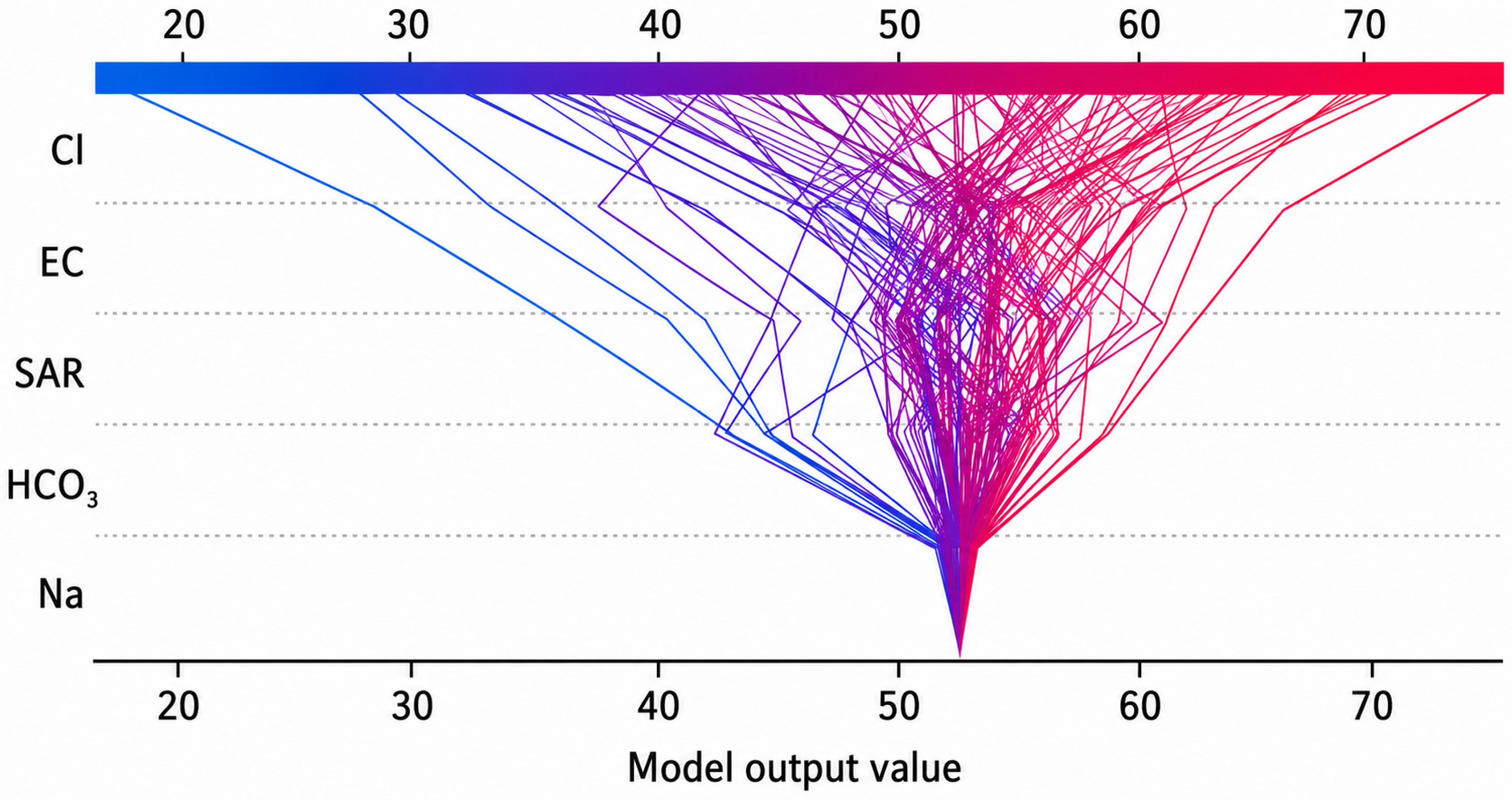
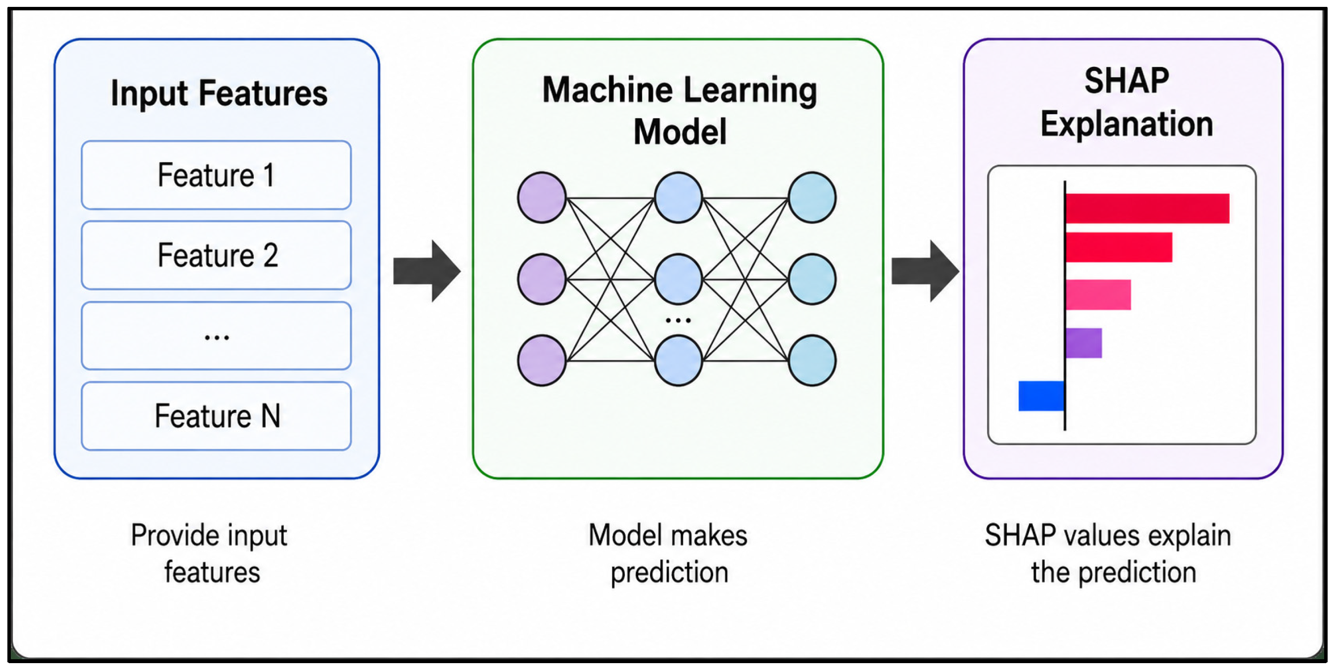
The SHAP-based interpretability workflow used in this study is illustrated in Figure 4.

SHAP was used strictly for model interpretation rather than predictive performance evaluation. SHAP contributions were interpreted as model-attribution measures and were not considered evidence of causal relationships. In particular, a large SHAP value indicates that the model relied strongly on a predictor when generating its output, but it does not establish an independent causal effect or a causal hydrochemical mechanism.

3. Results and Discussion

3.1. Statistical Summary of Physicochemical Parameters

Descriptive statistics for the measured water-quality parameters are presented in

Table 3. Descriptive Statistics of Water Quality Parameters.

Parameter	Min	Max	Mean	Std	Skewness	Kurtosis
pH	6.43	9.22	7.34	0.38	1.36	5.28
T (°C)	11.00	19.80	15.56	1.95	−0.16	−0.61
O2 (mg/L)	0.39	9.32	4.92	2.69	−0.10	−1.26
EC (µS/cm)	400.00	5160.00	1570.10	817.60	1.49	3.31
Turbidity (NTU)	0.13	39.30	4.72	5.80	3.25	14.10
HCO3 (mg/L)	91.50	945.50	310.06	123.63	2.05	7.36
SO4 (mg/L)	22.09	691.14	116.77	111.19	2.99	10.79
Ca (mg/L)	27.20	680.00	142.43	101.48	2.50	8.63
Mg (mg/L)	0.24	156.00	28.33	32.82	1.79	2.99
Cl (mg/L)	142.00	710.00	350.97	134.94	0.82	0.33
K (mg/L)	0.13	151.69	13.78	28.83	4.49	19.39
Na (mg/L)	37.29	414.00	167.18	51.74	1.29	4.86
TH (mg/L CaCO3)	92.24	1755.28	472.33	295.21	1.53	3.04

. pH ranged from 6.43 to 9.22 (mean = 7.34 ± 0.38), indicating predominantly neutral to slightly alkaline conditions, whereas EC ranged from 400 to 5160 µS/cm (mean = 1570.10 ± 817.60 µS/cm), indicating substantial variability in groundwater mineralization. Both parameters showed positive skewness (1.363 and 1.492, respectively), reflecting a limited number of relatively high values.

The major cations also exhibited considerable variability. Ca²⁺ had a mean concentration of 142.43 ± 101.48 mg/L and pronounced positive skewness (2.499), while Mg²⁺ and Na⁺ averaged 28.33 ± 32.82 and 167.18 ± 51.74 mg/L, respectively. K⁺ showed the strongest skewness (4.488) and highest kurtosis (19.387), with a mean of 13.78 ± 28.83 mg/L, indicating a small number of exceptionally high concentrations. Among the major anions, Cl⁻ and HCO₃⁻ had relatively high mean concentrations of 350.97 ± 134.94 and 310.06 ± 123.63 mg/L, respectively, while SO₄²⁻ averaged 116.77 ± 111.19 mg/L. The positive skewness observed for HCO₃⁻ (2.053) and SO₄²⁻ (2.997) further indicates considerable spatial heterogeneity.

Turbidity ranged from 0.13 to 39.30 NTU (mean = 4.72 ± 5.80 NTU) and showed strong positive skewness (3.25) and kurtosis (14.10), indicating mostly low values with a limited number of highly turbid samples. Total hardness ranged from 92.24 to 1755.28 mg/L as CaCO₃ (mean = 472.33 ± 295.21 mg/L), while temperature and dissolved oxygen averaged 15.56 ± 1.95 °C and 4.92 ± 2.69 mg/L, respectively.

Overall, the relatively high EC, together with the elevated Cl⁻ and HCO₃⁻ concentrations, is consistent with substantial water–rock interaction and evaporative concentration under semi-arid conditions, particularly in aquifer systems influenced by carbonate and evaporite mineral dissolution [2,3]. Similar hydrochemical characteristics have been reported for semi-arid Algerian groundwater systems, including the Bouhamdane Basin [49] and the M’sila region [16]. The pronounced positive skewness observed for several parameters indicates a limited number of high-concentration observations and highlights the spatial heterogeneity of groundwater chemistry. These observations were retained because elevated concentrations may represent genuine hydrochemical variability relevant to irrigation-water quality and subsequent IWQI reconstruction. Therefore, observations were not excluded solely on the basis of their distributional characteristics; instead, their influence was considered within the subsequent modelling framework through the predefined validation and feature-selection procedures.

3.2. Irrigation Water Quality Index (IWQI) Assessment

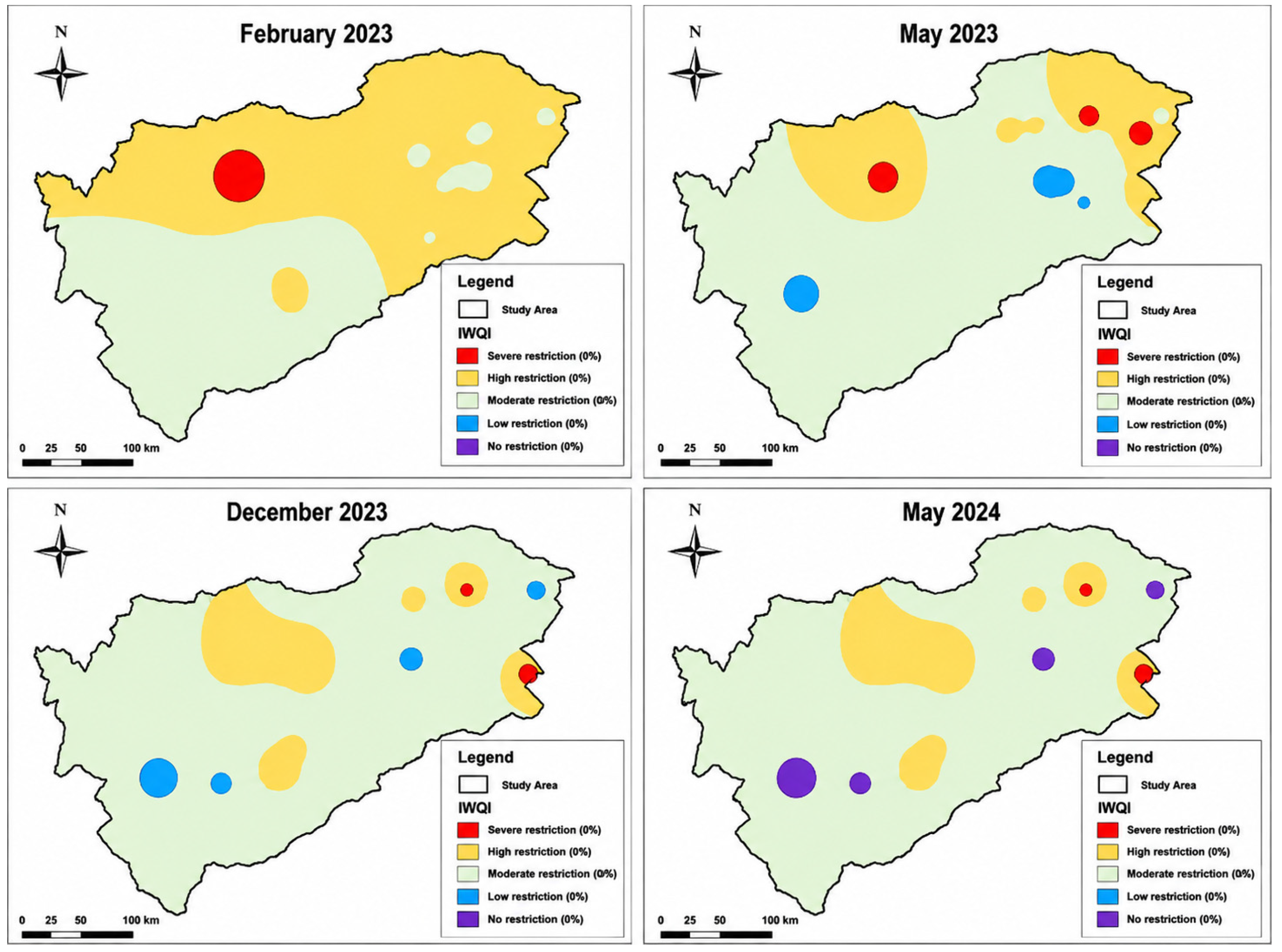
IWQI values ranged from 28.72 to 76.28 (mean = 56.16 ± 10.55). The class distribution was as follows: 56% moderate restriction, 28% high restriction, 8% severe restriction, and 8% low restriction (none unrestricted). According to the IWQI classification of Meireles et al. [5], samples in the moderate-restriction class (55–70) require appropriate soil management, leaching practices, and selection of tolerant crops. Conversely, 36% of samples in the high- or severe-restriction categories (IWQI < 55), located in areas under high agricultural and urban pressure, impose severe restrictions. The spatial distribution (Figure 5) confirms localized quality degradation, correlated with anthropogenic contamination signatures.

The observed IWQI range (28.72–76.28; mean = 56.16 ± 10.55) and class distribution are broadly consistent with IWQI assessments reported in comparable semi-arid groundwater systems. Nefla et al. [18] reported IWQI values predominantly in the moderate-to-high restriction range for a coastal Algerian aquifer, while M’nassri et al. [17] found similar class distributions in a Tunisian semi-arid context. The complete absence of the ‘no restriction’ class (IWQI > 85) in the Sedrata dataset indicates that no sampled groundwater is suitable for unrestricted irrigation use, which has direct implications for agricultural management: even the 8% of samples classified under low restriction (IWQI 70–85) require careful crop selection and periodic leaching to prevent long-term soil degradation [4,6]. The 36% of samples classified under high or severe restriction (IWQI < 55) represent a significant agronomic risk, particularly for salt-sensitive crops, and may require blending with higher-quality water sources or adoption of pressure-compensating irrigation technologies to mitigate soil sodification and structural damage. The spatial concentration of low-IWQI samples in zones of elevated agricultural and urban activity, as confirmed by the spatial distribution map (Figure 5), underscores the need for targeted monitoring and site-specific water management strategies in the Sedrata Plain.

3.3. Pearson Correlation and Multicollinearity Analysis

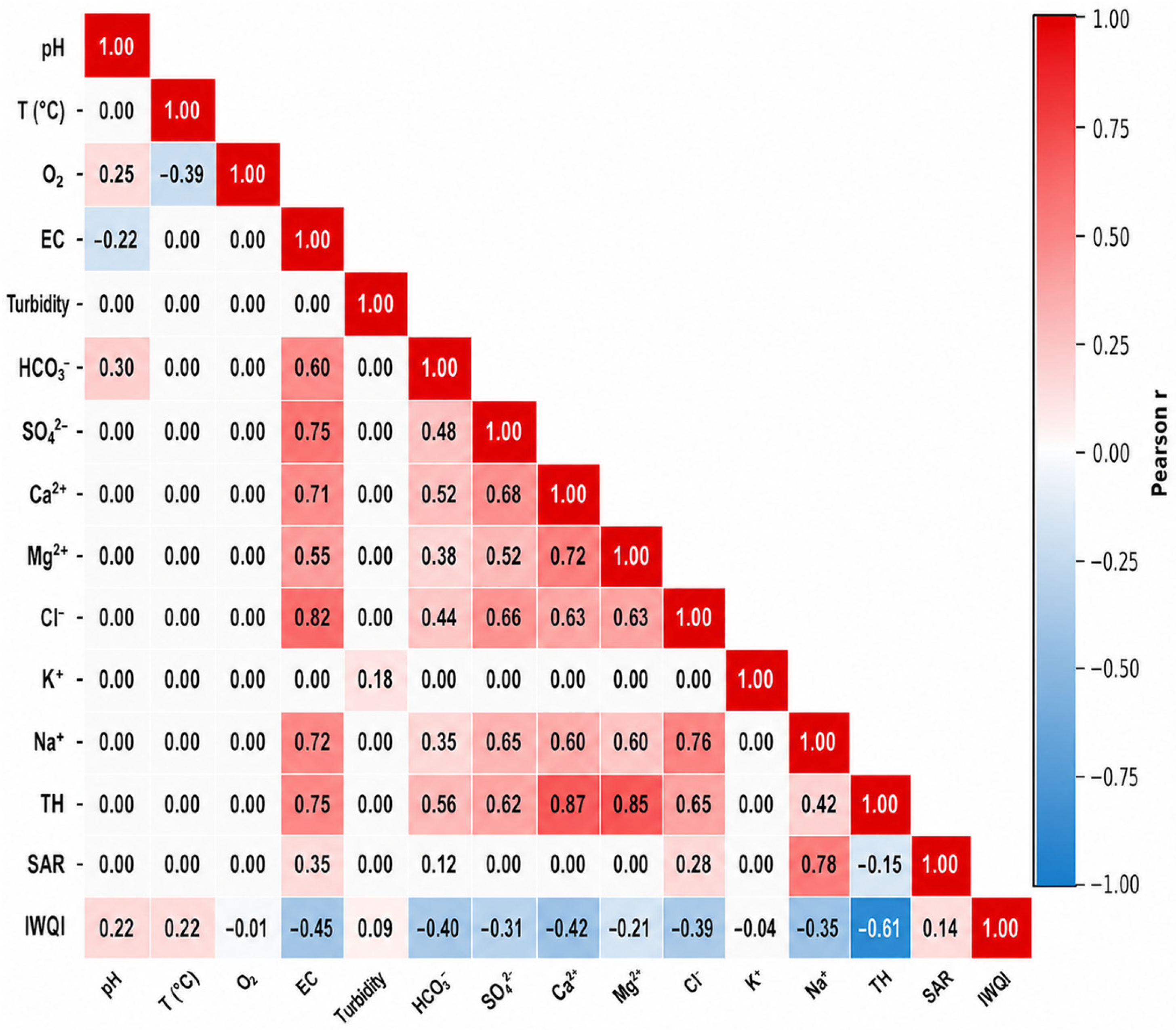
Pearson correlation analysis was performed to assess linear associations between the 14 candidate physicochemical predictors and IWQI across the 100 groundwater observations (Figure 6). Because IWQI is a deterministic composite index derived from several hydrochemical parameters, these correlations were interpreted as statistical associations rather than independent evidence of predictive importance or hydrogeochemical causality. EC, Na⁺, Cl⁻, HCO₃⁻, and SAR are directly incorporated into the IWQI formulation (Table 2), whereas TH is not [5].

The strongest negative correlations with IWQI were observed for HCO₃⁻ (r = −0.691), TH (r = −0.680), EC (r = −0.647), Ca²⁺ (r = −0.625), and Cl⁻ (r = −0.589). SO₄²⁻ (r = −0.526), Na⁺ (r = −0.351), and Mg²⁺ (r = −0.312) also showed negative associations. In contrast, pH and temperature exhibited weak positive correlations (r = +0.22 for both), while SAR showed a weak positive and non-significant correlation (r = +0.157, p = 0.120). O₂, turbidity, and K⁺ showed negligible linear associations with IWQI (r = −0.01, +0.09, and −0.04, respectively). The weak Pearson correlation of SAR does not necessarily indicate low predictive relevance, as its contribution to IWQI is governed by the predefined quality-rating and weighting functions and may involve nonlinear or threshold-dependent behaviour.

Strong inter-predictor correlations were observed among salinity- and mineralization-related variables. EC correlated strongly with Cl⁻ (r = 0.82), SO₄²⁻ (r = 0.75), TH (r = 0.75), and Na⁺ (r = 0.72), reflecting their co-occurrence in the mineralized groundwater system. VIF analysis identified perfect multicollinearity among Ca²⁺, Mg²⁺, and TH (VIF = ∞), consistent with the mathematical derivation of TH from Ca²⁺ and Mg²⁺ concentrations (Equation (2)). Consequently, Ca²⁺ and Mg²⁺ were excluded from the subsequent RFECV candidate pool, while TH was retained as the composite hardness indicator. Overall, these results highlight substantial predictor interdependence and support the use of nonlinear machine-learning models to capture relationships and interactions not adequately represented by pairwise linear correlations.

VIF analysis within the training partitions revealed perfect collinearity among Ca²⁺, Mg²⁺, and TH (VIF = ∞), consistent with the mathematical derivation of TH from Ca²⁺ and Mg²⁺ concentrations (Equation (2)). Consequently, Ca²⁺ and Mg²⁺ were excluded from the subsequent RFECV candidate pool, while TH was retained as the composite hardness indicator. No other predictor exhibited perfect multicollinearity.

3.4. Feature Selection via Nested RFECV

Nested Recursive Feature Elimination with Cross-Validation (RFECV) was performed independently within the four LOCO training partitions to identify a parsimonious predictor set for IWQI reconstruction. Although the selected subsets varied slightly among folds, EC, Na⁺, Cl⁻, HCO₃⁻, and SAR were consistently retained across all four LOCO folds, forming a stable five-predictor core.

Following multicollinearity screening, Ca²⁺ and Mg²⁺ were excluded from the RFECV candidate pool, while TH was retained as the composite hardness indicator. Although TH showed a strong correlation with IWQI (r = −0.680), it was not consistently selected across the four LOCO folds, which may reflect redundancy with other mineralization-related predictors and its derivation from Ca²⁺ and Mg²⁺ concentrations.

The consistent selection of EC, Na⁺, Cl⁻, HCO₃⁻, and SAR is partly expected because these variables are direct components of the computed IWQI. Their repeated selection therefore indicates stable predictive relevance for reconstructing the deterministic index rather than independent evidence of causal hydrochemical control. This predictor core is broadly consistent with previous ML-based IWQI studies in semi-arid environments. Azlaoui et al. [11] identified EC, Na⁺, and SAR among the most important predictors in an XGBoost-SHAP framework, while Hussein et al. [14] reported Na⁺ and EC as dominant predictors across multiple ML algorithms.

The final five-predictor configuration provides a parsimonious representation of the original 14-variable candidate pool while retaining routinely measured or readily derived parameters, supporting its practical use in groundwater monitoring and IWQI reconstruction. This reduction in dimensionality is also consistent with the principle of parsimonious model design in environmental modelling [40]. Accordingly, EC, Na⁺, Cl⁻, HCO₃⁻, and SAR were retained for subsequent model comparison and SHAP-based interpretation.

3.5. Machine-Learning Performance Under LOCO Validation

All machine-learning performance values reported in this section correspond to out-of-sample results obtained from the held-out test campaign of each LOCO fold (n = 25), rather than to training-set performance or to a random 80/20 split. Within each outer LOCO fold, preprocessing, VIF-based multicollinearity screening, RFECV feature selection, scaling, hyperparameter optimisation, and model fitting were carried out entirely within the corresponding training partition (n = 75); the held-out campaign was excluded from every stage of model development. LOCO was therefore adopted as the primary evaluation framework, assessing model generalisation to an unseen sampling campaign within the observed study period, rather than universal generalisation, transferability to other aquifers, or operational readiness.

Fold-level LOCO R² values for all six models are presented in

Table 4. Fold-level LOCO R² for the six evaluated models using the midpoint-based IWQI formulation.

Model	February 2023	May 2023	December 2023	May 2024
XGBoost	0.684	0.741	0.624	0.879
Gradient Boosting	0.668	0.724	0.512	0.854
KNN	0.589	0.747	0.665	0.759
Random Forest	0.657	0.673	0.573	0.821
SVR	0.364	0.680	0.769	0.643
MLR (5 IWQI components)	0.112	0.651	0.755	0.733

. XGBoost obtained the highest R² in three of the four held-out campaigns, ranging from 0.624 (December 2023) to 0.879 (May 2024); the exception occurred in December 2023, when SVR (R² = 0.769) numerically exceeded XGBoost. Gradient Boosting followed a pattern broadly similar to XGBoost, whereas KNN, Random Forest, and SVR displayed comparatively larger fold-to-fold fluctuations. MLR showed the widest range of all models, from R² = 0.112 (February 2023) to R² = 0.755 (December 2023), reflecting pronounced instability of the linear reconstruction across campaigns.

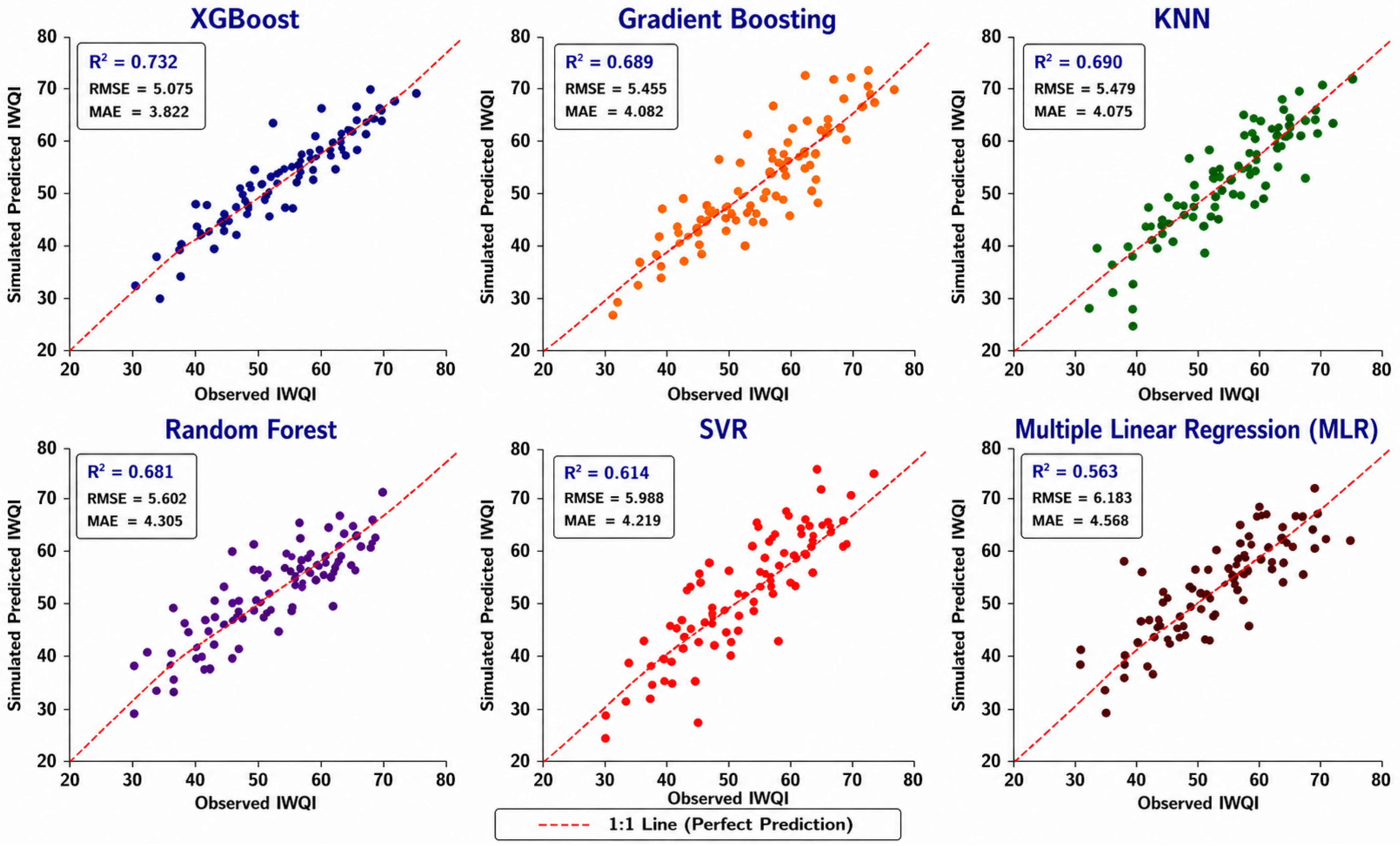
Averaged across the four held-out campaigns, XGBoost showed the highest mean LOCO performance (R² = 0.732 ± 0.109; RMSE = 5.075 ± 1.403; MAE = 3.822 ± 0.998;

Table 5. Summary of LOCO performance metrics.

Model	R2 (Mean ± SD)	RMSE (Mean ± SD)	MAE (Mean ± SD)
XGBoost	0.732 ± 0.109	5.075 ± 1.403	3.822 ± 0.998
Gradient Boosting	0.689 ± 0.142	5.455 ± 1.578	4.082 ± 1.032
KNN	0.690 ± 0.079	5.479 ± 0.655	4.075 ± 0.305
Random Forest	0.681 ± 0.103	5.602 ± 1.433	4.305 ± 1.202
SVR	0.614 ± 0.175	5.988 ± 0.864	4.219 ± 0.618
MLR (5 components)	0.563 ± 0.304	6.188 ± 1.276	4.568 ± 0.988

). Gradient Boosting and KNN achieved similar mean R² values (0.689 ± 0.142 and 0.690 ± 0.079, respectively), closely followed by Random Forest (0.681 ± 0.103), whereas SVR (0.614 ± 0.175) and MLR (0.563 ± 0.304) obtained the lowest mean R² values. Because only four outer folds were available, these values should be regarded as descriptive statistics summarising variability across the observed campaigns rather than as estimates of population-level uncertainty, and no significance testing was performed. Accordingly, XGBoost is described as the numerically strongest-performing model, showing the highest mean LOCO performance among the evaluated algorithms, rather than as statistically superior to its competitors.

Campaign-level variability was not restricted to XGBoost. SVR ranged from R² = 0.364 (February 2023) to 0.769 (December 2023), corresponding to a spread of 0.405 R² units, whereas MLR displayed the largest fold-level range among the evaluated models (0.643 R² units). These fluctuations indicate that model performance and relative ranking were not fully consistent across campaigns. Such variation may plausibly reflect differences in the hydrochemical composition of the held-out campaign relative to the corresponding training data; however, this interpretation remains a plausible explanation rather than an established causal effect.

Because IWQI is a deterministic composite index computed from a fixed set of hydrochemical parameters, the task addressed in this section represents surrogate reconstruction of a mathematically derived index rather than prediction of an independent environmental outcome. The IWQI scoring procedure applies piecewise quality-rating functions (q_i) across predefined parameter-quality ranges (Equation (4)), resulting in nonlinear and threshold-like relationships between the hydrochemical inputs and the resulting index. The relatively narrow performance range among the four nonlinear models (mean R² = 0.681–0.732), compared with the substantially lower mean R² obtained by MLR (0.563), is consistent with the piecewise structure of the IWQI formulation. A single linear combination of the five input variables may therefore not fully represent the threshold-dependent relationships embedded in the index. This finding does not imply that MLR is inherently unsuitable; rather, MLR provides a meaningful linear baseline using the same five predictors, whereas the underlying mathematical structure of IWQI is not necessarily well represented by a simple linear function.

The comparable performance of KNN (mean R² = 0.690) and Random Forest (0.681) relative to XGBoost (0.732) indicates that instance-based and bagging ensemble methods were also able to capture nonlinear structure in the predictor space, although with somewhat lower mean performance and/or cross-fold consistency. KNN’s sensitivity to local sample density [17] may partly explain its fold-level variability when campaign-specific hydrochemical shifts altered the distribution of nearest neighbours in the held-out set. Random Forest, which relies on bootstrap aggregation and randomized feature selection, also captured nonlinear relationships but showed a lower performance ceiling than the boosting-based models [9]. SVR showed lower and more variable performance (mean R² = 0.614; range = 0.364–0.769), which may reflect the sensitivity of RBF-kernel SVR to kernel and regularization settings when modelling nonlinear, piecewise-structured targets, particularly under the relatively small outer training partition (n = 75).

The relative performance ordering observed in the present LOCO evaluation, XGBoost ≈ Gradient Boosting > KNN ≈ Random Forest > SVR > MLR, is broadly comparable with rankings reported in previous ML-based IWQI studies, although the magnitude of performance differences varies across datasets and validation designs [14,16]. Several previous studies reported substantially higher R² values (e.g., 0.85–0.97) using random train–test partitioning rather than grouped or campaign-level validation [11,14]. Because repeated observations from the same wells may be distributed across random training and test subsets, such partitioning can yield optimistic estimates of generalisation when observations within wells are not independent. Direct numerical comparison between the present LOCO-based results and these studies should therefore be interpreted with caution, given differences in validation strategy, dataset size, sampling design, predictor set, and IWQI formulation.

Within this context, the XGBoost model achieved a mean LOCO R² of 0.732, compared with 0.563 for MLR, indicating an observed advantage of the nonlinear tree-based model for reconstructing the piecewise IWQI target from the available hydrochemical predictors under the present campaign-level validation framework. This advantage should be interpreted in relation to the specific dataset, predictor set, IWQI formulation, and validation strategy used in this study, rather than as evidence of universal superiority or broad generalisability.

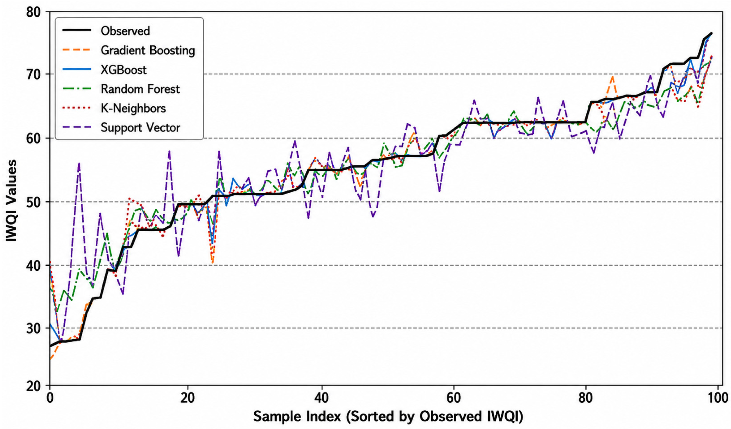
Figure 7 illustrates the agreement between computed and reconstructed IWQI values for the six evaluated models under the LOCO validation framework.

Taken together, the fold-level and aggregate LOCO results support the selection of XGBoost as the final model for the SHAP-based interpretability analysis presented in the following section. XGBoost was selected as the final model because it achieved the highest numerical performance under the strict LOCO framework, but this result should be interpreted as evidence of comparatively better IWQI reconstruction within the present Sedrata dataset and validation design, not as proof of universal superiority or external generalisation.

Figure 8 further illustrates the distributional reproduction of IWQI values across the five nonlinear machine-learning models.

3.5.1. Statistical Comparisons

Paired t-tests based on the four fold-level LOCO R² values were used as an exploratory comparison between XGBoost and the other evaluated models. Because only four paired folds were available and multiple pairwise comparisons were performed, these tests are exploratory rather than confirmatory, and the reported p-values are unadjusted for multiplicity. XGBoost showed a numerical advantage over Gradient Boosting (mean ΔR² = +0.043), but this difference was not statistically significant (t = 1.833, p = 0.164). Differences between XGBoost and SVR (mean ΔR² = +0.118, t = 1.147, p = 0.335), KNN (mean ΔR² = +0.042, t = 1.092, p = 0.355), and MLR (mean ΔR² = +0.169, t = 1.151, p = 0.333) were likewise not statistically significant. Only the comparison between XGBoost and Random Forest reached significance in the unadjusted paired t-test (mean ΔR² = +0.051, t = 5.796, p = 0.010); given the small number of outer folds (df = 3) and the absence of correction for multiple comparisons, this result should be interpreted cautiously and not as evidence of general statistical superiority.

Accordingly, XGBoost is described as achieving the highest mean LOCO performance among the evaluated models; its numerical advantage was statistically significant only relative to Random Forest in the unadjusted paired comparison, and not relative to Gradient Boosting, KNN, SVR, or MLR. These results should not be interpreted as evidence that XGBoost is statistically superior to all competing models. Because only four outer LOCO folds were available (n = 4; df = 3), statistical power was limited, and the exploratory nature of these comparisons should be kept in mind throughout the remainder of this study.

Notably, MLR outperformed XGBoost in the December 2023 held-out campaign (R² = 0.755 vs. 0.624), illustrating pronounced campaign-to-campaign variability in relative model performance. This observation indicates that the numerical advantage of XGBoost at the mean level does not guarantee superior performance in every individual campaign. The stronger performance of MLR in December 2023 may indicate that the linear structure was better aligned with the hydrochemical configuration of that specific campaign than the nonlinear models evaluated, although this interpretation remains observational rather than causally established. This pattern is consistent with the broader finding that campaign-specific conditions, rather than algorithmic complexity alone, can be an important factor shaping reconstruction accuracy in a given LOCO fold; it argues against selecting a single model based solely on mean performance and suggests that campaign-adaptive or ensemble strategies may warrant future investigation.

The paired t-test results comparing XGBoost with the other evaluated models are presented in

Table 6. Paired t-test results comparing XGBoost with the other models based on fold-level LOCO R² (df = 3, two-tailed).

Comparison	Mean ΔR2	t	p	Unadjusted Significance
XGBoost vs. GB	+0.043	1.833	0.164	No (n.s.)
XGBoost vs. RF	+0.051	5.796	0.010	Yes (p < 0.05)
XGBoost vs. SVR	+0.118	1.147	0.335	No (n.s.)
XGBoost vs. KNN	+0.042	1.092	0.355	No (n.s.)
XGBoost vs. MLR	+0.169	1.151	0.333	No (n.s.)

Notes: (n.s.) not significant; p < 0.05 in the unadjusted paired t-test.

.

3.5.2. Leave-One-Well-Out (LOWO) Validation Results

Leave-One-Well-Out (LOWO) cross-validation was performed as a secondary grouped validation analysis to complement the primary campaign-level LOCO results. Whereas LOCO evaluates model generalisation across held-out sampling campaigns, LOWO evaluates generalisation to monitoring wells that were entirely excluded from model development: in each of the 25 folds, all four observations from one monitoring well were held out, while observations from the remaining 24 wells were used for training. This design ensures that measurements from the same well are never simultaneously present in the training and test partitions. Because each held-out set contained only four observations, RMSE and MAE were treated as the primary fold-level error metrics, while fold-level R² was interpreted with caution.

For XGBoost, the mean LOWO RMSE across the 25 held-out wells was 4.475 ± 2.943 IWQI units (median = 3.891; range: 0.298–9.847), with a mean LOWO MAE of 3.485 ± 2.387 IWQI units and an aggregate R² of 0.914 calculated from all 100 held-out LOWO predictions. The other models produced mean LOWO RMSE values of 2.527 (Gradient Boosting), 2.712 (SVR), 2.780 (Random Forest), 2.807 (MLR), and 2.886 (KNN) IWQI units, with corresponding aggregate LOWO R² values of 0.912, 0.825, 0.878, 0.900, and 0.868, respectively. Notably, Gradient Boosting 2.4.1 achieved a substantially lower mean LOWO RMSE (2.527 IWQI units) than XGBoost (4.475 ± 2.943 IWQI units), indicating that the best-performing algorithm depends on the validation strategy used. XGBoost is therefore identified as the best-performing model under the primary LOCO validation framework specifically, rather than as the universally optimal algorithm across all validation contexts.

Taken together, the LOCO and LOWO results provide complementary, though not equivalent, evidence regarding the internal transferability of the trained XGBoost surrogate within the Sedrata Plain dataset. LOCO evaluates campaign-level generalisation within the observed study period, the ability to reconstruct IWQI values for hydrochemical conditions associated with a held-out sampling campaign, whereas LOWO evaluates within-aquifer spatial generalisation to monitoring well locations not represented during model development. XGBoost’s mean RMSE under LOCO (5.075 ± 1.403 IWQI units) and under LOWO (4.475 ± 2.943 IWQI units) are numerically similar in central tendency; however, the substantially larger variability observed under LOWO (SD = 2.943 vs. 1.403) indicates that spatial generalisation to individual wells is considerably less consistent than campaign-level generalisation, and the two validation schemes should not be regarded as formally equivalent. This pattern of internal transferability is a necessary but not sufficient condition for broader applicability: it indicates that the model is not simply memorising training-set patterns, but it does not establish transferability to aquifer systems with different hydrochemical regimes, geological settings, or IWQI distributions. External transferability to geographically distinct datasets remains untested and is discussed further as a limitation in Section 3.8 and Section 3.9.

3.5.3. Secondary Reference: Random 80/20 Split

For comparison with previous studies that used conventional random data partitioning, a random 80/20 train–test split (random_state = 42) was performed as a secondary, descriptive reference analysis. Under this split, XGBoost yielded R² = 0.698, RMSE = 4.791, and MAE = 3.474, while MLR produced R² = 0.256, RMSE = 7.522, and MAE = 5.181. These results are reported solely as secondary reference values and should not be regarded as evidence of robust model generalisation. Because the dataset comprises repeated observations from the same 25 monitoring wells across four campaigns, observations from a given well can occur in both the training and test subsets under random splitting; this can produce optimistic performance estimates relative to the grouped LOCO framework, which explicitly prevents observations from the held-out campaign from contributing to model development or evaluation.

The random_state = 42 used for this random partition was independent of the fixed seed = 0 used for stochastic model procedures within the primary LOCO and secondary LOWO analyses: random_state = 42 controlled the train–test split, whereas seed = 0 ensured the reproducibility of stochastic algorithm behaviour. The two values therefore serve distinct methodological purposes and were not intended to be identical.

3.5.4. Comparison with Previous IWQI/WQI Machine-Learning Studies

To place the present LOCO-based results within the broader ML-based water-quality-index literature,

Table 7. Comparison of the present LOCO-based results with previous ML-based IWQI/WQI studies.

Study/Reference	Study Area	ML Approach	Validation Strategy	Reported R2 (Best Model)	Notes
Present study (LOCO)	Sedrata Plain, Algeria	XGBoost	Grouped, campaign-level LOCO (n = 4 folds)	0.732 ± 0.109	Strict held-out campaign; no well overlap between train/test
Present study (80/20)	Sedrata Plain, Algeria	XGBoost	Random 80/20 (secondary reference)	0.698	Reported only as a descriptive reference; not primary result
Azlaoui et al. [11]	Aïn Oussera plain, Djelfa, Algeria	XGBoost + SHAP	Conventional train–test partitioning	0.95 (RMSE = 3.22)	EC and SAR identified as dominant SHAP predictors
Hussein et al. [14]	Naama region, Algeria	XGBoost, SVR, KNN	Conventional train–test partitioning	≈0.97	Na+ and EC among the most influential predictors
Zegaar et al. [16]; M’nassri et al. [17]; Nefla et al. [18]; Panagiotou et al. [19]	Various semi-arid Algerian and Tunisian aquifers	Various (XGBoost, RF, ANN, SVR)	Predominantly conventional/random partitioning	≈0.85–0.97 (range across studies)	Figures as reported in the original studies; not independently re-verified against primary sources

consolidates the performance metrics reported in Section 3.5.3 alongside comparable studies previously cited in this manuscript. This comparison is intended to make the methodological contrast between grouped, campaign-level validation and conventional random partitioning explicit and quantifiable, rather than only asserted narratively.

The XGBoost surrogate developed in the present study achieved a mean LOCO R² of 0.732 ± 0.109, which is numerically lower than the R² values reported by Azlaoui et al. [11] (0.95) and Hussein et al. [14] (≈0.97), as well as those reported in other semi-arid Algerian and Tunisian studies (≈0.85–0.97). This difference may be partly attributable to differences in validation design, as the cited studies predominantly relied on conventional or random train–test partitioning, under which repeated observations from the same monitoring wells may be allocated to both the training and test subsets. Such partitioning can yield optimistic estimates of model generalisation when observations from the same wells are not independent. In contrast, the present study used Leave-One-Campaign-Out (LOCO) validation as the primary evaluation strategy, ensuring that all observations from the held-out campaign were excluded from model training. The secondary random 80/20 split performed in the present study (Section 3.5.3) yielded an XGBoost R² of 0.698, which was lower than the mean LOCO R² of 0.732, although the two values are not directly equivalent because they arise from different evaluation designs. The remaining differences relative to the literature values reported in

Table 8. Baseline performance comparison for the standard Meireles IWQI formulation.

Method/Reference	Validation	R2	RMSE	MAE
Deterministic IWQI calculation	Direct IWQI calculation	1.000	0.000	0.000
MLR (5 IWQI components)	80/20 (random_state = 42)	0.256	7.522	5.181
MLR (5 IWQI components)	LOCO (mean ± SD)	0.563 ± 0.304	6.188 ± 1.276	4.568 ± 0.988
XGBoost	80/20 (random_state = 42)	0.698	4.791	3.474
XGBoost	LOCO (mean ± SD)	0.732 ± 0.109	5.075 ± 1.403	3.822 ± 0.998

may also reflect variation in dataset size, predictor set, sampling density, and IWQI formulation across studies.

The consistency of EC and Na⁺, together with related salinity indicators such as SAR and Cl⁻, as important predictors across Azlaoui et al. [11], Hussein et al. [14], and the present study (Section 3.4) supports the relevance of the retained five-predictor set despite differences in absolute reconstruction accuracy across validation frameworks. Overall, Table 8 indicates that the present results are broadly consistent with, although numerically more conservative than, previously reported ML-based IWQI/WQI studies. The lower performance values should therefore be interpreted in the context of the stricter campaign-level validation strategy, as well as differences in datasets, predictor sets, sampling designs, and IWQI formulations, rather than being interpreted as evidence of generally inferior model capability.

3.6. Baseline Performance Comparison

A baseline performance comparison was performed to place the machine-learning results within the context of the deterministic IWQI formulation. Direct IWQI calculation provides a deterministic reference, yielding R² = 1.000, RMSE = 0, and MAE = 0 when the prescribed qiq_i values and weighting coefficients are applied according to Equations (4) and (5), because IWQI is defined as a fixed mathematical function of its five input components rather than as an independently measured environmental outcome. In comparison, XGBoost achieved a mean LOCO R² of 0.732 ± 0.109 (RMSE = 5.075 ± 1.403; MAE = 3.822 ± 0.998 IWQI units), whereas MLR using the same five IWQI-related predictors showed lower LOCO performance (R² = 0.563 ± 0.304; RMSE = 6.188 ± 1.276; MAE = 4.568 ± 0.988 IWQI units).

Framed against this deterministic reference, the lower performance of the machine-learning models should be interpreted as reflecting the challenge of reconstructing a deterministic, piecewise composite index from raw hydrochemical concentrations rather than as evidence of poor predictive performance for an independent environmental outcome. The difference between the deterministic IWQI reference (R² = 1.00) and the best-performing ML surrogate (XGBoost mean LOCO R² = 0.732) may have several non-exclusive explanations. First, the IWQI formulation combines multiple parameter-specific quality-rating functions and weighting terms, including piecewise relationships across predefined quality bands (Table 1), resulting in a nonlinear mapping that must be approximated from a finite set of observations. Second, the LOCO framework deliberately withholds an entire sampling campaign from model training, so the surrogate must generalize to hydrochemical conditions that may differ from those represented in the training campaigns. The deterministic IWQI equation, in contrast, can be applied directly to the held-out observations without requiring statistical generalization.

The mean LOCO RMSE of 5.075 IWQI units corresponds to approximately 5.1% of the full 0–100 IWQI scale. Because IWQI restriction classes span intervals of different widths, whether a reconstruction error changes the assigned water-quality class depends on the proximity of the true IWQI value to a class boundary rather than on RMSE alone. No class-reassignment analysis was performed in the present study; therefore, the implications of the observed reconstruction error for categorical irrigation-water classification should be considered a potential direction for future work rather than an established finding.

Overall, the XGBoost surrogate achieved substantially better LOCO performance than the linear baseline while remaining below the deterministic reference, as expected for an approximate statistical reconstruction of a mathematically defined index. The model may therefore have potential for rapid screening of IWQI from EC, Na⁺, Cl⁻, HCO₃⁻, and SAR measurements. However, this potential remains provisional and requires independent external validation across additional sampling campaigns, wells, and hydrogeological settings before transferability beyond the present dataset can be established.

3.7. Model Interpretability via SHAP Analysis

To interpret the final XGBoost model and quantify the relative contribution of the selected predictors to IWQI reconstruction, SHAP (SHapley Additive exPlanations) values were computed for the model refitted on all 100 observations using the five retained predictors: EC, Na⁺, Cl⁻, HCO₃⁻, and SAR. Because refitting used the complete dataset, including the campaigns held out during LOCO evaluation, the SHAP analysis characterises the behaviour of the final fitted model rather than providing an out-of-sample explainability assessment; this distinction is acknowledged as a methodological limitation in Section 3.8. Throughout this section, SHAP values are interpreted strictly as measures of model attribution and reliance, i.e., how strongly the fitted XGBoost model depends on each predictor when reconstructing IWQI, and not as evidence of independent causal hydrogeochemical relationships.

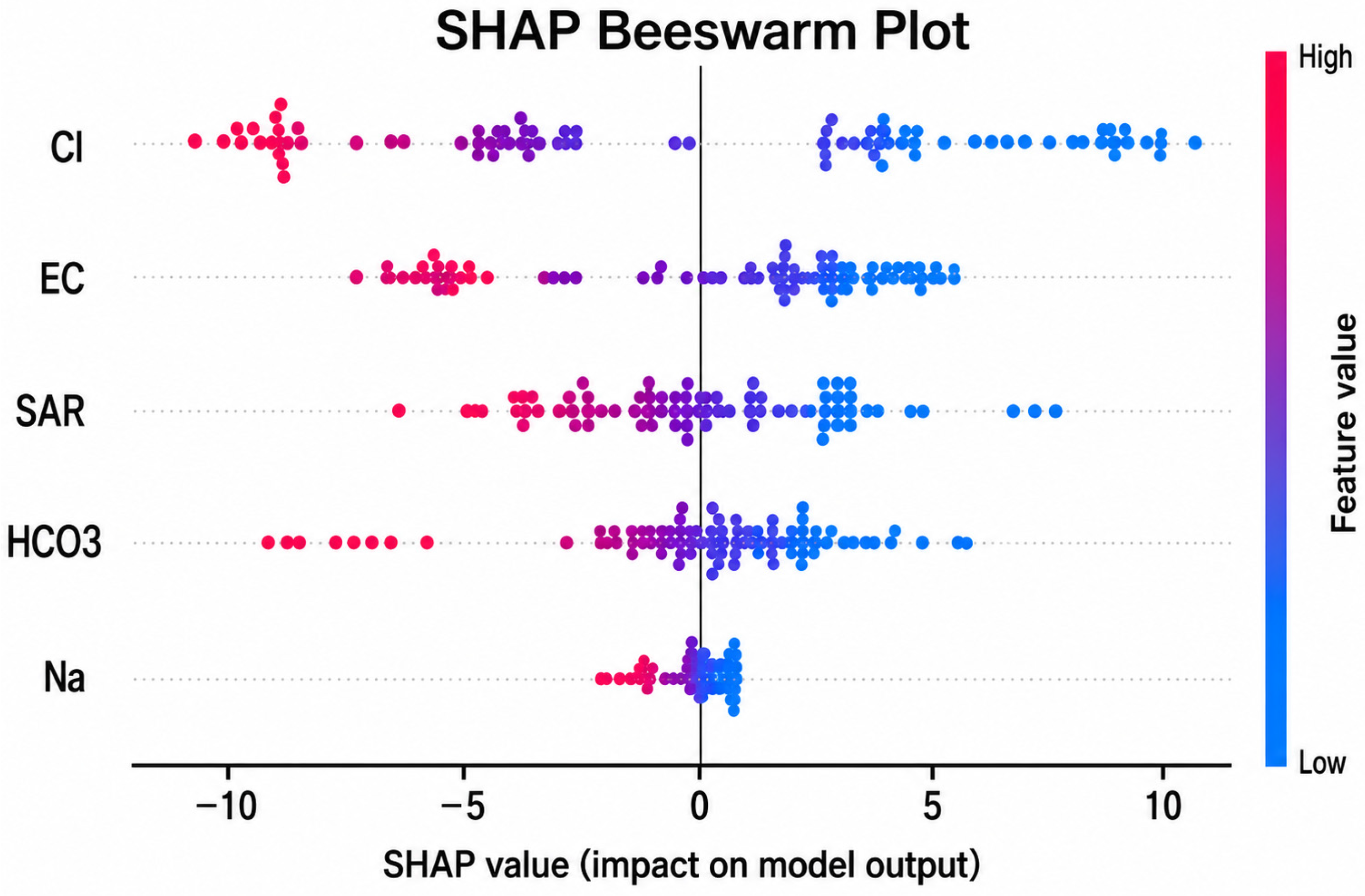
Figure 9 presents the SHAP beeswarm plot for the five predictors, ranked by mean absolute SHAP value; each point represents one observation, its horizontal position indicating the magnitude and direction of that predictor’s contribution to the predicted IWQI, and its colour indicating the corresponding feature value (blue = low, red = high) [48]. Positive SHAP values push the prediction toward higher IWQI, negative values toward lower IWQI, and predictors positioned farther from zero exert greater influence on the model output.

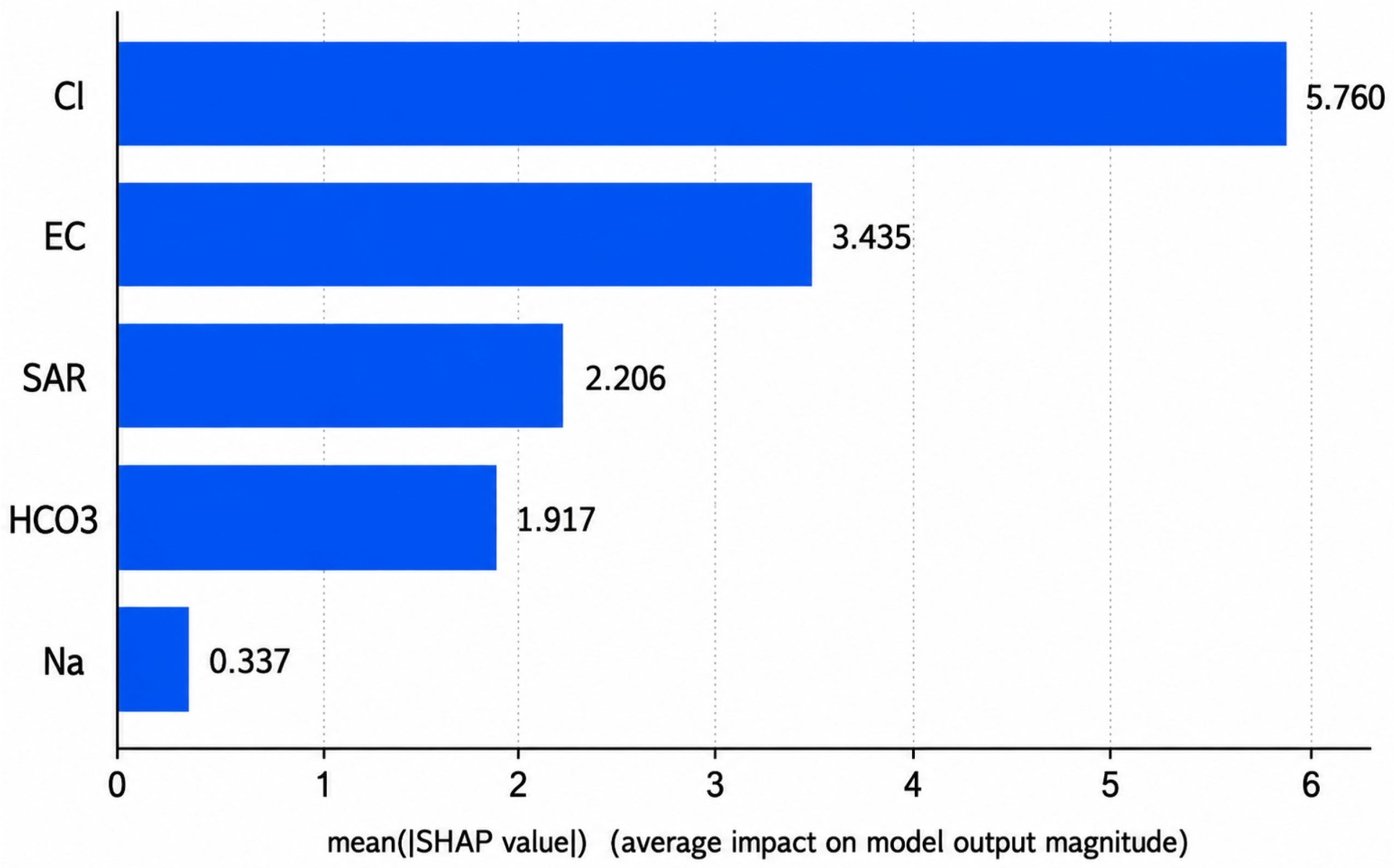
Global feature importance (Figure 10), based on mean absolute SHAP values, summarises the predictors’ average contribution to the predicted IWQI irrespective of direction, yielding the hierarchy Cl⁻ (5.760) > EC (3.435) > SAR (2.206) > HCO₃⁻ (1.917) > Na⁺ (0.337). This ranking is complementary to the feature-selection results reported in Section 3.4: RFECV identifies which predictors are retained for modelling, whereas SHAP quantifies how strongly the final fitted XGBoost model relies on each retained predictor when generating its predictions.

The SHAP decision plot (Figure 11) provides an observation-level view of how the five predictors jointly contribute to individual IWQI predictions, with each line tracing the cumulative contribution from the model’s expected value to the final prediction for one observation. Because positive and negative contributions from different predictors can partially offset one another, observations with similar final predicted IWQI values may follow different attribution pathways, reflecting the nonlinear, interaction-based structure of the XGBoost model and underscoring that individual predictions arise from the combined contribution of Cl⁻, HCO₃⁻, EC, SAR, and Na⁺ rather than from any single predictor acting independently.

Because several selected predictors are direct or indirect components of the IWQI formulation, high SHAP importance indicates that the XGBoost model relies strongly on a predictor when reconstructing IWQI values in the present dataset; it does not establish that predictor as an independent hydrogeochemical driver of irrigation-water quality. SHAP values quantify feature contributions to individual model predictions and can be aggregated to characterize global feature importance. The prominence of Cl⁻ and EC is consistent with the importance of salinity-related variables in irrigation-water assessment, but this pattern should be interpreted as model attribution rather than evidence of a causal mechanism or of any single constituent independently controlling water quality.

The SHAP-derived hierarchy (Cl⁻ > EC > SAR > HCO₃⁻ > Na⁺) is broadly consistent with feature-importance patterns reported in comparable ML-based IWQI studies, although the specific ordering remains dataset- and model-dependent. Azlaoui et al. [11] identified EC and Na⁺ among the dominant contributors to XGBoost-based predictions in a semi-arid Algerian aquifer, while Li et al. [52] reported a predominance of salinity-related variables in SHAP-based interpretation of XGBoost water-quality models. These comparisons support the relevance of salinity-related predictors while also indicating that their relative importance may vary among datasets and model configurations.

Cl⁻ showed the highest mean absolute SHAP value in the present study (mean |SHAP| = 5.760). Its relatively high concentration (mean = 350.97 mg/L; range = 142–710 mg/L) provides substantial variation in the predictor space; however, concentration range alone does not determine SHAP importance, which also depends on the fitted model structure and interactions among predictors. Conversely, Na⁺ showed a comparatively low mean absolute SHAP contribution (mean |SHAP| = 0.337), despite being a direct component of the IWQI formulation. This may partly reflect its correlation with EC and Cl⁻ (r = 0.72 and 0.76, respectively), indicating that information associated with Na⁺ may overlap with that represented by other predictors available to the model. This interpretation should be regarded as a possible explanation rather than evidence of an independent effect.

Similarly, the positive SHAP association observed for SAR despite its weak and non-significant Pearson correlation with IWQI (r = +0.157, p = 0.120) illustrates that SHAP attributions should not be interpreted as direct extensions of pairwise correlations. SAR enters the IWQI formulation through a parameter-specific quality-rating function, and its model contribution may therefore vary across observations and predictor combinations. The nonlinear tree-based structure of XGBoost can represent such relationships, whereas Pearson correlation summarizes only linear pairwise association. XGBoost is specifically designed as a tree-boosting framework capable of modelling nonlinear relationships through sequentially fitted decision trees.

Together, these findings demonstrate the complementary roles of RFECV-based feature selection and SHAP-based explainability in the present deterministic composite-index reconstruction task. RFECV identifies a parsimonious predictor set within the specified training procedure, whereas SHAP characterizes how the fitted XGBoost model distributes attribution among the retained predictors. These provide distinct but complementary forms of model interpretation and should not be regarded as evidence of independent hydrogeochemical causality.

Overall, the SHAP analysis provides an attribution-based description of the final five-predictor XGBoost model at both the global and observation levels. Because the same predictor configuration (EC, Na⁺, Cl⁻, HCO₃⁻, and SAR) underlies the feature-selection, modelling, and SHAP stages, the resulting interpretation is internally consistent. Nevertheless, the SHAP results remain specific to the fitted model, dataset, predictor set, and validation framework and should not be interpreted as evidence of universal predictor importance across aquifers or datasets.

3.8. Limitations

Several limitations should be considered when interpreting the present results. The dataset comprised 100 groundwater observations from 25 open wells monitored during four campaigns over a 15-month period (February 2023–May 2024). Although this design captures seasonal variability within the Sedrata Plain, it does not represent longer-term inter-annual hydrochemical changes associated with climate variability, prolonged drought, aquifer depletion, or changes in agricultural practices. The sampled wells were also limited to shallow open wells (approximately 3–25 m), and therefore deeper confined or semi-confined aquifer horizons were not represented. Accordingly, the trained XGBoost surrogate should not be assumed to maintain its reconstruction accuracy under hydrochemical conditions substantially outside the range represented in the study dataset.

The validation results also have important scope limitations. The primary LOCO evaluation yielded R² = 0.732 ± 0.109, RMSE = 5.075 ± 1.403, and MAE = 3.822 ± 0.998 IWQI units, whereas the secondary LOWO analysis yielded a mean RMSE of 4.475 ± 2.943 IWQI units. LOWO provides complementary evidence of within-aquifer generalisation, but each held-out well contained only four observations, making fold-level estimates sensitive to well-specific hydrochemical conditions. These results therefore support internal generalisation within the sampled Sedrata Plain rather than external generalisation to other aquifer systems. Transfer to aquifers with different lithological and hydrochemical characteristics, or to alternative IWQI formulations with different parameter bands and weighting schemes, would require local retraining and independent validation. External validation and formal applicability-domain assessment were not performed.

Finally, the target IWQI is a deterministic composite index derived partly from the same physicochemical variables used as predictors (EC, Na⁺, Cl⁻, HCO₃⁻, and SAR); therefore, the ML task represents surrogate reconstruction of IWQI rather than prediction of an independent environmental outcome. Similarly, SHAP values describe model attribution and should not be interpreted as causal hydrogeochemical evidence. The RFECV procedure and predefined hyperparameter search cannot guarantee identification of the globally optimal predictor subset or model configuration. In addition, formal uncertainty quantification and prediction intervals were not estimated for individual reconstructions. Future studies should therefore evaluate the framework using larger multi-year datasets, independent external sites, broader applicability-domain analysis, and formal uncertainty-quantification approaches before considering wider transfer or operational use.

3.9. Future Research Directions and Recommendations

Future research should first evaluate the five-predictor XGBoost framework using larger, multi-year, and geographically independent datasets. Independent external validation across hydrogeologically comparable semi-arid aquifers in Algeria and the broader Maghreb region would provide a stronger assessment of model transferability and help determine whether the observed predictor-importance pattern is specific to the Sedrata Plain or is reproducible across comparable aquifer systems. Such evaluations should be accompanied by applicability-domain assessment to identify observations falling outside the chemical space represented in the Sedrata training data. Where substantial distributional shifts are identified, local retraining or domain-adaptation approaches may be preferable to direct model transfer.

Methodological development should also focus on formal uncertainty quantification, including conformal prediction or prediction-interval approaches, so that individual IWQI reconstructions can be accompanied by estimates of predictive reliability. Future studies should further assess the stability of the five-predictor configuration using alternative feature-selection criteria, such as permutation importance, SHAP-based selection, or mutual information. Given the four-campaign structure of the present dataset, additional sampling campaigns would also be required to investigate seasonally aware or time-series modelling approaches and to determine whether temporal information improves campaign-level generalisation. Incorporating relevant spatial covariates, such as water-table depth, soil characteristics, and proximity to agricultural areas, could additionally help represent spatial heterogeneity that is not fully captured by the five hydrochemical predictors.

Following successful external validation and uncertainty assessment, the framework could be further investigated for practical applications in groundwater monitoring and irrigation-water management. Potential applications include prioritising wells for detailed laboratory analysis, supporting spatial IWQI mapping, and integrating the surrogate with routine field or sensor-based measurements for preliminary screening. However, such applications should remain conditional on demonstrated external validity, applicability-domain reliability, and adequate uncertainty characterisation. Future work could also make the modelling pipeline publicly available to facilitate independent evaluation and adaptation in other data-scarce semi-arid aquifer systems.

4. Conclusions

This study developed an interpretable machine-learning framework for approximating the Irrigation Water Quality Index (IWQI) in the phreatic aquifer of the Sedrata Plain, northeastern Algeria, using a reduced hydrochemical predictor set and 100 groundwater observations collected across four seasonal campaigns. The integration of nested RFECV, comparison of five nonlinear machine-learning algorithms with a linear baseline (MLR), campaign-based Leave-One-Campaign-Out (LOCO) validation, and SHAP analysis provided a structured framework for assessing both surrogate reconstruction performance and model attribution.

The RFECV procedure consistently retained EC, Na⁺, Cl⁻, HCO₃⁻, and SAR across the four LOCO folds, resulting in a five-predictor configuration that is also consistent with the mathematical structure of the IWQI formulation. Among the evaluated models, XGBoost achieved the highest mean LOCO performance, with R² = 0.732 ± 0.109, RMSE = 5.075 ± 1.403 IWQI units, and MAE = 3.822 ± 0.998 IWQI units. The paired comparison between XGBoost and Random Forest reached the conventional unadjusted significance threshold (p = 0.010); however, this result should be interpreted cautiously because only four outer LOCO folds were available and no multiplicity correction was applied. Accordingly, XGBoost can be considered the best-performing model within the primary LOCO validation framework, rather than a universally superior algorithm.

SHAP analysis provided an interpretable representation of how the final XGBoost model used the retained predictors, with Cl⁻, EC, and SAR showing the highest mean absolute SHAP contributions. Their prominence is consistent with their role within the IWQI formulation; however, SHAP values represent model attribution rather than independent causal hydrogeochemical evidence. Overall, the results demonstrate the feasibility of combining data-driven feature selection, nonlinear machine-learning modelling, grouped cross-validation, and explainability for IWQI surrogate reconstruction in the studied semi-arid groundwater system.

The findings are broadly consistent with previously reported ML-based IWQI/WQI studies in semi-arid Algerian and Tunisian settings, while also highlighting an important methodological distinction. The hydrochemical characteristics and IWQI classification patterns observed in the Sedrata Plain are comparable to those reported for the Bouhamdane Basin, the M’sila region, and other regional aquifer systems. The prominence of salinity-related predictors, particularly Cl⁻ and EC, in the present SHAP analysis is also broadly consistent with the importance of EC, Na⁺, and related salinity indicators reported in previous ML-based studies. However, the mean LOCO R² obtained in the present study (0.732 ± 0.109) is numerically lower than the higher R² values reported in studies using conventional or random train–test partitioning (approximately 0.85–0.97; Table 8). This difference may partly reflect the stricter campaign-level validation strategy adopted here, in addition to differences in datasets, predictor sets, sampling designs, and IWQI formulations. The comparison therefore indicates broad consistency with previous literature while avoiding direct equivalence between results obtained under different validation frameworks.

The proposed framework should nevertheless be regarded as internally validated within the Sedrata Plain. External validation using geographically independent datasets, together with applicability-domain assessment and formal uncertainty quantification, is required before transfer to other aquifer systems or operational use. Future studies should therefore focus on larger multi-year datasets and independent sites to determine whether the predictive performance and predictor-attribution patterns of the five-predictor XGBoost framework remain stable under different hydrogeological and hydrochemical conditions.

References

1. Jasechko, S.; Seybold, H.; Perrone, D.; Fan, Y.; Shamsudduha, M.; Taylor, R.G.; Fallatah, O.; Kirchner, J.W. Rapid groundwater decline and some cases of recovery in aquifers globally. Nature 2024, 625, 715–721. [Google Scholar] [CrossRef] [Scilit] [PubMed]
2. Yadav, P.; Sreekesh, S.; Nandimandalam, J.R. Groundwater Quality and Its Suitability in the Semi-Arid River Basin in India: An Analysis of Hydrogeochemical Processes Using Multivariate Statistics. Environ. Model. Assess. 2025, 30, 625–646. [Google Scholar] [CrossRef] [Scilit]
3. Khan, I.; Singh, A.; Jamal, Y. Hydrogeochemical Dynamics of Groundwater in the Punjab Region of the Indo-Gangetic Plains: An Entropy-Weighted and Geochemical Modeling Approach. Earth Syst. Environ. 2026, 10, 1437–1460. [Google Scholar] [CrossRef] [Scilit]
4. Muniz, D.H.F.; Malaquias, J.V.; Lima, J.E.F.W.; Oliveira-Filho, E.C. Proposal of an irrigation water quality index (IWQI) for regional use in the Federal District, Brazil. Environ. Monit. Assess. 2020, 192, 607. [Google Scholar] [CrossRef] [Scilit] [PubMed]
5. Meireles, A.C.M.; de Andrade, E.M.; Chaves, L.C.G.; Frischkorn, H.; Crisostomo, L.A. A new proposal of the classification of irrigation water. Rev. Ciênc. Agron. 2010, 41, 349–357. [Google Scholar] [CrossRef] [Scilit]
6. Ayers, R.S.; Westcot, D.W. Water Quality for Agriculture; Food and Agriculture Organization of the United Nations: Rome, Italy, 1985; Volume 29, Available online: https://www.academia.edu/download/5596796/c-110101.pdf (accessed on 22 August 2026).
7. Zahi, F.; Mecibah, I.; Drouiche, A.; AbdelRahman, M.A.E.; Medjani, F.; Djidel, M.; Scopa, A. Application of an integrated GIS-AHP water quality index to evaluate the groundwater suitability for irrigation in a coastal aquifer in northeastern Algeria. PLoS Water 2026, 5, e0000511. [Google Scholar] [CrossRef]
8. Friedman, J.H. Greedy function approximation: A gradient boosting machine. Ann. Stat. 2001, 29, 1189–1232. [Google Scholar] [CrossRef] [Scilit]
9. Breiman, L. Random Forests. Mach. Learn. 2001, 45, 5–32. [Google Scholar] [CrossRef] [Scilit]
10. Yan, X.; Zhang, T.; Du, W.; Meng, Q.; Xu, X.; Zhao, X. A comprehensive review of machine learning for water quality prediction over the past five years. J. Mar. Sci. Eng. 2024, 12, 159. [Google Scholar] [CrossRef] [Scilit]
11. Azlaoui, M.; Karef, S.; Foufou, A.; Haied, N.; Azlaoui, N.; Rabehi, A.; Habib, M.; Zeddouri, A. Machine Learning-Based Prediction of Irrigation Water Quality Index with SHAP Interpretability: Application to Groundwater Resources in the Semi-Arid Region, Algeria. Water 2026, 18, 959. [Google Scholar] [CrossRef] [Scilit]
12. Lundberg, S.M.; Lee, S.-I. A unified approach to interpreting model predictions. Adv. Neural Inf. Process. Syst. 2017, 30, 4765–4774. [Google Scholar]
13. Al-Jamimi, H.A.; Saleh, T.A. Explainable AI via PSO-optimized CatBoost and SHAP analysis: A case study on nanocomposite membrane performance. Neural Comput. Appl. 2026, 38, 501. [Google Scholar] [CrossRef] [Scilit]
14. Hussein, E.E.; Derdour, A.; Zerouali, B.; Almaliki, A.; Wong, Y.J.; Santos, M.B.-D.L.; Ngoc, P.M.; Hashim, M.A.; Elbeltagi, A. Groundwater quality assessment and irrigation water quality index prediction using machine learning algorithms. Water 2024, 16, 264. [Google Scholar] [CrossRef] [Scilit]
15. Gaagai, A.; Aouissi, H.A.; Bencedira, S.; Hinge, G.; Athamena, A.; Heddam, S.; Gad, M.; Elsherbiny, O.; Elsayed, S.; Eid, M.H.; et al. Application of water quality indices, machine learning approaches, and GIS to identify groundwater quality for irrigation purposes: A case study of Sahara Aquifer, Doucen Plain, Algeria. Water 2023, 15, 289. [Google Scholar] [CrossRef] [Scilit]
16. Zegaar, A.; Telli, A.; Ounoki, S.; Shahabi, H. Interpretable Machine Learning Models for Irrigation Sustainability: Groundwater Quality Prediction in M’sila, Algeria. Environ. Model. Assess. 2025, 30, 399–416. [Google Scholar] [CrossRef] [Scilit]
17. M’nassri, S.; El Amri, A.; Nasri, N.; Majdoub, R. Estimation of irrigation water quality index in a semi-arid environment using data-driven approach. Water Supply 2022, 22, 5161–5175. [Google Scholar] [CrossRef] [Scilit]
18. Nefla, L.; Bergal, A.; Boumaraf, W.; Gheid, S.; Bouksiba, C.; Khammar, H.; Celico, F.; Nasri, H.; Gaagai, A.; Elsayed, S.; et al. Integrated GIS-machine learning approach to irrigation water quality assessment in coastal aquifers. Sci. Rep. 2026, 16, 3894. [Google Scholar] [CrossRef] [Scilit] [PubMed]
19. Panagiotou, C.F.; Konstantinou, C.; Chekirbane, A. A generalized machine learning approach for cost-effective monitoring of irrigation suitability: A demonstration case in El Fahs aquifer (Tunisia). Groundw. Sustain. Dev. 2024, 27, 101324. [Google Scholar] [CrossRef] [Scilit]
20. Roberts, D.R.; Bahn, V.; Ciuti, S.; Boyce, M.S.; Elith, J.; Guillera-Arroita, G.; Hauenstein, S.; Lahoz-Monfort, J.J.; Schröder, B.; Thuiller, W.; et al. Cross-validation strategies for data with temporal, spatial, hierarchical, or phylogenetic structure. Ecography 2017, 40, 913–929. [Google Scholar] [CrossRef] [Scilit]
21. Hastie, T.; Friedman, J.; Tibshirani, R. The Elements of Statistical Learning; Springer Series in Statistics; Springer: New York, NY, USA, 2001. [Google Scholar] [CrossRef] [Scilit]
22. Halimi, S. Resources and Trial of Integrated Water Management in Wadi Cherf/Sedrata Watershed (Northeastern Algeria). Master’s Thesis, Badji Mokhtar Annaba University, Annaba, Algeria, 2008. [Google Scholar]
23. Monographie de la Wilaya de Souk Ahras; Souk Ahras, Algeria, 2019. Available online: https://souk-ahras.mta.gov.dz/wp-content/uploads/sites/34/2022/03/Monographie-de-la-wilaya-de-Souk-Ahras-2019.pdf (accessed on 30 August 2026).
24. Bellazi, M.A. Diagnostic de la Pollution de Certains Milieux Aquatiques de la Région de Souk Ahras. PhD Thesis, University of Souk Ahras, Souk-Ahras, Algeria, 2021. [Google Scholar]
25. David, L. Étude Géologique des Monts de la Haute Medjerda; Publications du Service de la Carte Géologique de l’Algérie, Nouvelle Série, Bulletin No. 11; Service de la Carte Géologique de l’Algérie: Alger, Algeria, 1956; 304p. [Google Scholar]
26. Dubourdieu, G. Étude Géologique de la Région de l’Ouenza (Confins Algéro-Tunisiens); Nouvelle Série, Bulletin No. 10; Publications du Service de la Carte Géologique de l’Algérie: Alger, Algérie, 1956; 659p. [Google Scholar]
27. Voûte, C. Essai de Synthese de L’histoire Geologique des Environs d’Ain Fakroun, Ain Babouche et des Régions Limitrophes; Planches; Service Géologique: Alger, Algeria, 1967. [Google Scholar]
28. Vila, J.-M. La Chaîne Alpine d’Algérie Orientale et Des Confins Algéro-Tunisiens. Ph.D. Thesis, Université Pierre-et-Marie-Curie, Paris, France, 1977. [Google Scholar]
29. Vila, J.-M. Note sur la stratigraphie et la tectonique des Beni Salah, Souk Ahras, Algérie. Bull. Soc. Géol. Fr. 1977, 19, 437–445. [Google Scholar]
30. Chabbi, M. Étude Géologique et Structurale de la Région de Sédrata (Wilaya de Souk Ahras). Ph.D. Thesis, Université Badji Mokhtar, Annaba, Algeria, 2017. [Google Scholar]
31. APHA. Standard Methods for the Examination of Water and Waste? Water; American Health Association: Washington, DC, USA, 1995. [Google Scholar]
32. Reza, S.K.; Haldar, A.; Khan, S.K.; Rahman, F.H. Validation of water quality parameters using ion balancing and electrochemical approaches: A case study. Int. J. Environ. Anal. Chem. 2025, 105, 6681–6700. [Google Scholar] [CrossRef] [Scilit]
33. Hossain, M.; Patra, P.K. Hydrogeochemical characterisation and health hazards of fluoride enriched groundwater in diverse aquifer types. Environ. Pollut. 2020, 258, 113646. [Google Scholar] [CrossRef] [Scilit] [PubMed]
34. Richards, L.A. Diagnosis and improvement of saline and alkali soils. Soil Sci. 1954, 78, 154. [Google Scholar] [CrossRef] [Scilit]
35. Pedregosa, F.; Varoquaux, G.; Gramfort, A.; Michel, V.; Thirion, B.; Grisel, O.; Blondel, M.; Prettenhofer, P.; Weiss, R.; Dubourg, V.; et al. Scikit-learn: Machine Learning in Python. J. Mach. Learn. Res. 2011, 12, 2825–2830. [Google Scholar]
36. Kuhn, M.; Johnson, K. Nonlinear Regression Models. In Applied Predictive Modeling; Springer: New York, NY, USA, 2013; pp. 141–171. [Google Scholar] [CrossRef] [Scilit]
37. Imneisi, I.B. Using The Irrigation Water Quality Index to Evaluate of Some Water Resources in Al-Abyar-Ghut Al-Sultan Area NE Libya. Sci. J. Univ. Benghazi 2021, 34, 6. [Google Scholar] [CrossRef] [Scilit]
38. Dancey, C.P.; Reidy, J. Statistics Without Maths for Psychology; Pearson/Prentice Hall: Upper Saddle River, NJ, USA, 2007. [Google Scholar]
39. O’brien, R.M. A Caution Regarding Rules of Thumb for Variance Inflation Factors. Qual. Quant. 2007, 41, 673–690. [Google Scholar] [CrossRef] [Scilit]
40. Hair, J.F., Jr.; Black, W.C.; Babin, B.J.; Anderson, R.E. Multivariate Data Analysis, 7th ed.; Pearson Prentice Hall: Upper Saddle River, NJ, USA, 2010. [Google Scholar]
41. Guyon, I.; Elisseeff, A. An introduction to variable and feature selection. J. Mach. Learn. Res. 2003, 3, 1157–1182. [Google Scholar] [CrossRef] [Scilit]
42. Granitto, P.M.; Furlanello, C.; Biasioli, F.; Gasperi, F. Recursive feature elimination with random forest for PTR-MS analysis of agroindustrial products. Chemom. Intell. Lab. Syst. 2006, 83, 83–90. [Google Scholar] [CrossRef] [Scilit]
43. Julian, J.; Dewantara, A.B.; Wahyuni, F. Design of machine learning-based water quality prediction system with recursive feature elimination cross-validation. J. Infotel 2023, 15, 249–255. [Google Scholar] [CrossRef] [Scilit]
44. Chan, Y.H. Biostatistics 104: Correlational analyses. Singap. Med. J. 2003, 44, 614–619. [Google Scholar]
45. Cortes, C.; Vapnik, V. Support-vector networks. Mach. Learn. 1995, 20, 273–297. [Google Scholar] [CrossRef] [Scilit]
46. Chai, T.; Draxler, R.R. Root mean square error (RMSE) or mean absolute error (MAE)—Arguments against avoiding RMSE in the literature. Geosci. Model Dev. 2014, 7, 1247–1250. [Google Scholar] [CrossRef] [Scilit]
47. Jeong, J.G.; Ryu, Y.M.; Lee, E.H. Development of XAI-Based Explainable Planning Management for Chl-a Reduction. Water 2025, 18, 7. [Google Scholar] [CrossRef] [Scilit]
48. Varma, S.; Simon, R. Bias in error estimation when using cross-validation for model selection. BMC Bioinform. 2006, 7, 91. [Google Scholar] [CrossRef] [Scilit] [PubMed]
49. Singha, C.; Rana, V.K.; Pham, Q.B.; Nguyen, D.C.; Łupikasza, E. Integrating machine learning and geospatial data analysis for comprehensive flood hazard assessment. Environ. Sci. Pollut. Res. 2024, 31, 48497–48522. [Google Scholar] [CrossRef] [Scilit] [PubMed]
50. Willmott, C.J.; Matsuura, K. Advantages of the mean absolute error (MAE) over the root mean square error (RMSE) in assessing average model performance. Clim. Res. 2005, 30, 79–82. [Google Scholar] [CrossRef] [Scilit]
51. Tibshirani, R.; James, G.; Witten, D.; Hastie, T. Introduction to Statistical Learning. 2013. Available online: https://www.academia.edu/download/63575299/Introduction_to_Statistical_Learning_201720200609-32130-1u6aguu.pdf (accessed on 25 August 2026).
52. Li, W.; Deng, M.; Liu, C.; Cao, Q. Analysis of key influencing factors of water quality in Tai Lake Basin based on XGBoost-SHAP. Water 2025, 17, 1619. [Google Scholar] [CrossRef] [Scilit]
Figure 1. Geographical location of the study area and the groundwater sampling sites.
Water 18 02215 g001
Figure 2. Geological map of the study area. Geological framework. 1. Recent, 2. Villafranchian, 3. Pliocene, 4. Argillaceous Miocene, 5. Sandy Miocene, 6. Glauconite Miocene, Numidian Nappe: 7. Miocene, 8. Oligocene, Tellian Nappe: 9. Ypresian-Lutetian, 10. Paleocene, Sellaoua and North Aurès Units: 11. Maastrichtian, 12. Campanian, 13. Coniacian-Santonian, 14. Turonian, 15. Cenomanian, 16. Albian, 17. Barremian–Aptian and 18. Triassic, 19. The Roads. 20. Sampling Wells.
Water 18 02215 g002
Figure 3. Methodological framework for IWQI reconstruction, machine-learning model selection, and SHAP-based explainability of groundwater quality. Arrows indicate the workflow direction. In the RFECV panel (Method 3), colored circles represent candidate predictors evaluated at each elimination step, with colors used only to distinguish individual predictors; the ellipsis (…) denotes intermediate RFECV steps not shown. The five predictors retained after RFECV are listed on the right.
Water 18 02215 g003
Figure 4. Flowchart illustrating the SHAP value computation process for machine learning model interpretability. The ellipsis (…) denotes additional input features and intermediate model nodes that are not explicitly shown, while the colors are used to visually distinguish the different components of the workflow and SHAP contribution bars.
Water 18 02215 g004
Figure 5. Irrigation water quality index map of the study area.
Water 18 02215 g005
Figure 6. Pearson correlation coefficients between candidate predictors and IWQI.
Water 18 02215 g006
Figure 7. Computed versus reconstructed IWQI values for the six evaluated models under Leave-One-Campaign-Out (LOCO) validation.
Water 18 02215 g007
Figure 8. Distributional reproduction of IWQI values across the five nonlinear machine-learning models.
Water 18 02215 g008
Figure 9. SHAP beeswarm plot for the five selected predictors in the final XGBoost model.
Water 18 02215 g009
Figure 10. Global feature importance based on mean absolute SHAP values for the final XGBoost model.
Water 18 02215 g010
Figure 11. Decision plot showing cumulative contributions of individual variables to predictions for each groundwater sample observation. Lines are coloured according to the model output value, with blue representing lower predicted IWQI values and red representing higher predicted IWQI values.
Water 18 02215 g011