Tracing Water, Energy, and Pollution Pressures Driven by Chinese Household Food Demand Within the Water–Energy–Food Nexus

Abstract

Household food demand mobilizes water, energy, and pollutants throughout supply chains. Using China’s 2023 211-sector input-output table and environmental accounts, this study traces supply-chain water withdrawal, total energy consumption, and actual loads of chemical oxygen demand (COD), ammonia nitrogen (NH₃-N), total nitrogen (TN), and total phosphorus (TP) across 21 food-related sectors, including catering services (restaurants and related commercial food service activities). Household food demand induced 257 km³ of water withdrawal, 11.7 EJ of energy consumption, and the following pollutant loads: COD (1430 × 10⁴ t), NH₃-N (20.9 × 10⁴ t), TN (129 × 10⁴ t), and TP (20.5 × 10⁴ t). Plant-based primary foods led water withdrawal and nutrient loads; animal-source primary foods generated 59.5% of COD; catering services had the largest energy share. Upstream sectors contributed 53.2% of water withdrawal, 75.6% of energy consumption, 45.1% of COD, and 52.2–52.3% of nutrient loads. Covering 80% of each burden required 12 origin–destination links for water withdrawal, 56 for energy consumption, 5 for COD, and 11 for each nutrient, indicating dispersed energy attribution. Grain, other agricultural products, and livestock and other animal products recurred as multi-pressure hotspots. A conditional 20% reduction in their direct intensities lowered water withdrawal by 15.7%, energy consumption by 2.6%, COD by 10.3%, and nutrient loads by 16.1–16.2%. These findings support targeted water and pollution measures alongside broader upstream energy-efficiency action.

1. Introduction

Food systems connect water, energy, nutrient cycling, land, and pollution across production and consumption networks. Global water–energy–food (WEF) research treats these resources as coupled systems, while food footprint studies show large variation among products and production pathways [1,2,3,4]. Because household demand activates primary production, processing, industrial inputs, energy supply, and distribution, farm- or facility-level assessments can understate consumption-driven burdens and their implications for supply security and resilience [5].

In China, dietary transitions and the expansion of food supply chains have made the resource and environmental implications of food consumption increasingly cross-sectoral and transboundary. The increasing share of animal-source foods in Chinese diets has altered both the magnitude and composition of the water footprint associated with household food consumption [6]. Demand for meat and dairy products also connects domestic consumption with overseas land and water resources through feed production and international trade. Govoni et al. demonstrated that China’s consumption of animal protein is linked to land occupation, green water use, and deforestation risks associated with soybean production in Brazil [7]. Within China, the environmental burdens induced by food consumption extend beyond agriculture and food processing to upstream energy supply, industrial inputs, and distribution services [8]. A demand-based assessment is therefore needed to identify which sectors expand production, which production activities bear the associated environmental pressures, and which stages of the supply chain should be prioritized for intervention.

Water-quantity and water-quality pressures require distinct physical accounts. In this study, water withdrawal means the gross abstraction of water from surface water and groundwater sources for production activities. The analysis traces supply-chain water withdrawal induced by household food demand. This is not a complete blue–green–grey water footprint assessment. A blue water footprint generally measures consumptive use, including water incorporated into products or lost through evapotranspiration; green water generally refers to precipitation-derived soil moisture consumed by vegetation through evapotranspiration. Both lie outside this withdrawal-based boundary. By contrast, COD, NH₃-N, TN, and TP accounts record the actual mass of pollutants released from production activities. Retaining these pollutants as separate mass-based indicators avoids treating water abstraction and pollution as interchangeable quantities and preserves differences in their sources and management implications. Liang et al. showed that incorporating pollution constraints can alter the spatial prioritization of food-demand-driven water pressures in China [9]. Nutrient-extended input-output analysis demonstrates that food-related nitrogen losses arise through both direct agricultural production and indirect industrial inputs [10]. Foundational nitrogen footprint research connects consumption with reactive nitrogen losses across production and waste-management chains [11,12], while global studies identify fertilizer, feed, manure, and livestock production as major pathways shaping nitrogen and phosphorus pressures in food systems [13,14,15]. National food footprint studies further demonstrate how broader reactive nitrogen losses can be assigned to consumption [16,17]. The present study traces household-food-demand-induced NH₃-N and TN loads, but it is not a complete nitrogen footprint assessment because the satellite accounts do not cover all reactive nitrogen species, environmental media, or fate and transport pathways.

An integrated WEF view remains necessary because water, energy, and pollutants occur in different sectors and supply chain positions. Nexus methods range from biophysical and life-cycle approaches to optimization and economy-wide accounting [1,18], while Chinese regional studies add efficiency, spatial-econometric, and network analyses [19]. These approaches reveal regional coordination but do not directly trace specific food demand to supporting sectors; normalized composite indices may also obscure each pressure’s physical meaning. This study instead asks how large each burden is, where it occurs, how it propagates, and which sectors recur across pressures.

To trace the direct and indirect environmental burdens induced by final food demand through interindustry linkages, this study employs environmentally extended input-output (EEIO) analysis. EEIO links final demand to economy-wide production by augmenting monetary input-output accounts with environmental satellite accounts [20]. Detailed multi-regional input-output databases extend this logic across countries and sectors [21], and consumption-based footprint research shows how international trade separates final demand from production-side environmental pressure [22]. Single-region models quantify sectoral resource use attributable to final demand [23,24], whereas multi-regional models trace consumption-based attribution and spatial redistribution [25]. These models have also been used to identify cross-border virtual-water flows and their drivers [26]. Hybrid frameworks further improve the representation of complex food systems by incorporating physical agricultural flows and disaggregated consumption stages [27,28].

Multi-pressure comparison, transmission mechanisms, and governance screening are nevertheless often studied separately, although burdens differ by product and supply chain stage [16,17,29]. Sectoral attribution locates the full burden, while tier and structural-path methods trace propagation through input relationships [30,31]. Global evidence also links intervention opportunities to producer heterogeneity, diets, and feed substitution [2,4,32,33,34,35,36,37]. Most hotspot studies, however, use one indicator or fixed weights. Cumulative thresholds identify relevant processes [38], but their robustness for multi-pressure food chain screening remains insufficiently tested.

Using China’s 2023 national competitive input-output table, this study applies EEIO analysis to attribute household-food-demand-induced environmental pressures across national supply chains. Its objective is not to compare provinces, assess basin-level water scarcity, or reconstruct temporal evolution; the results therefore describe national intersectoral structure rather than spatial heterogeneity or temporal trends. Within this boundary, four questions are addressed. First, how much supply chain output, water withdrawal, total energy consumption, and COD, NH₃-N, TN, and TP loads are induced by Chinese household final demand for food in 2023? Second, how do these burdens differ among seven aggregated food demand groups and 21 detailed food sectors, and how are they distributed between final food sectors and successive upstream supply chain tiers? Third, which production origins, attribution linkages, and second-order structural paths transmit the principal burdens from final food demand to upstream suppliers? Fourth, which sectors recur across the indicator-specific high-contribution sets, how sensitive is this membership to cumulative thresholds of 70%, 80%, and 90%, and what conditional mitigation follows from 10%, 20%, and 30% reductions in their direct environmental intensities?

The study contributes by retaining six indicator-specific physical accounts rather than a composite score; linking 211 producing sectors to 21 food-related demand sectors through attribution, tier decomposition, and structural path analysis; and screening recurrent hotspots across six separate core sets with threshold sensitivity. This design identifies shared and pressure-specific priorities while distinguishing NH₃-N and TN load accounting from a complete nitrogen footprint.

2. Materials and Methods

This study integrates China’s 2023 211-sector national competitive input-output accounts with sectoral accounts for water withdrawal, total energy consumption, COD, NH₃-N, TN, and TP. Household food demand defines the final-demand boundary. The analysis quantifies total burdens; traces sectoral origins, tiers, and paths; and evaluates hotspot recurrence, threshold sensitivity, and conditional mitigation. Indicators remain in separate physical units. The national single-year model resolves neither geographic location nor temporal change.

2.1. System Boundary, Food Demand, and Data Sources

The analysis focuses on household final demand for food in China in 2023. The final-demand vector is constructed by summing the rural and urban household consumption columns in the national input-output table. A total of 21 food-related sectors are retained and aggregated into seven analytical categories: plant-based primary foods, animal-source primary foods, basic processed foods, animal-protein processed foods, other processed foods, beverages, and catering services. Feed products are excluded from the final-demand boundary because they are not purchased directly by households for consumption; however, their upstream contributions are represented through EEIO intermediate-input transactions with livestock and meat production sectors. Tobacco is excluded from household final demand. Catering services are included once as a final-demand service, while their purchases of agricultural and processed food products are traced through the intermediate-input matrix, thereby avoiding double counting. Within the official input-output classification, the “other agricultural products” sector is a mixed category containing edible agricultural commodities together with certain non-food cash crops and related agricultural products. It is retained in the baseline to avoid omitting edible household consumption. Further disaggregation is not performed because the official framework provides neither a finer interindustry transaction matrix nor matching environmental satellite accounts and internally consistent coefficients at that resolution. Splitting the sector using external product statistics would require unsupported allocation assumptions and could disrupt transaction balance, environmental-intensity consistency, and the reliability of supply chain attribution. The existing exclusion sensitivity test evaluates whether this mixed-sector boundary affects the main conclusions; it does not impose artificial subsectors. The same 21-sector and seven-group classification is used consistently throughout the analysis.

All 211 producing sectors are retained so that agricultural, feed, energy, chemical, packaging, transport, trade, and water supply inputs remain within the boundary. Economic and environmental accounts are matched nationally; pressure origins denote sectors, not locations. Direct household water and energy use and consumption-stage wastewater are excluded. Because the competitive table does not separate imported from domestic intermediate products, imports are assigned domestic production technologies and environmental intensities. Results, therefore, represent national supply chain attribution, not pressures located entirely in China or observed footprints in exporting economies. The main data sources, original coverage, and their use in the model are summarized in

Table 1. Main data sources, original coverage, and use in the model.

Account	2023 Data Source	Original Coverage	Treatment and Model Use
Economic accounts	National Bureau of Statistics of China, 2023 National Input-Output Table (competitive) [39]	211 product sectors; monetary values in 104 CNY	Intermediate use, total output, and rural and urban household consumption are extracted to construct A, L, and the food final-demand vector.
Water withdrawal	Ministry of Water Resources, 2023 China Water Resources Bulletin [40]	Agricultural, industrial, domestic, and ecological replenishment withdrawals; km3	A production water-withdrawal account is constructed; direct household use and ecological replenishment are excluded.
Total energy consumption	Department of Energy Statistics, National Bureau of Statistics of China, China Energy Statistical Yearbook 2024, Chapter 4, Table 4-4, “Total Energy Consumption by Sector” (2023 data) [41]	Industry-level total energy consumption, including producing sectors and residential use; source unit: 104 tce	Residential energy use is excluded. The published industry totals are concorded with the 211-sector input-output classification; where one statistical industry corresponds to multiple input-output sectors, its total is allocated in proportion to their 2023 sectoral output. Aggregate results are converted to EJ or PJ using 1 tce = 29.3076 GJ [42].
Water pollutants	Ministry of Ecology and Environment, 2023 Annual Report on Environmental Statistics [43]	Agricultural, industrial, and domestic sources of COD, NH3-N, TN, and TP; 104 t	The baseline includes agricultural and industrial sources that can be assigned directly to production; domestic sources are used in a boundary test.

Note: All economic and environmental accounts refer to 2023. Sectoral concordances, allocation weights, and data quality checks were applied when constructing the 211-sector satellite accounts.

.

2.2. Sectoral Mapping of Environmental Satellite Accounts

The water-withdrawal satellite account records gross abstraction from surface water and groundwater sources for production activities and uses 491 km³ of production-related water withdrawal as the control total. Agricultural water withdrawal totaling 367 km³ is allocated across crop production, forestry, livestock production, and aquaculture sectors. Of the 97.0 km³ of industrial water withdrawal, 49.0 km³ of once-through cooling water used in thermal and nuclear power generation is allocated separately to the relevant electricity-generation sectors, while the remaining volume is assigned to other industrial sectors. The public-service component of domestic-use water withdrawal, amounting to 26.7 km³, is allocated to the corresponding service sectors within the production system. Direct household water withdrawal of 64.3 km³ and ecological water replenishment of 35.4 km³ are excluded from the production-related water account. Because sector-specific observations are unavailable for all 211 sectors, each published aggregate is allocated among the corresponding sectors in proportion to their sectoral output in 2023. This allocation preserves official aggregate control totals while introducing uncertainty into sector-level attribution, which is further discussed in Section 4.6. The resulting EEIO estimates therefore represent supply chain water withdrawal induced by household food demand, not consumptive blue water use or a blue water footprint. They do not quantify water incorporated into products, evapotranspiration, or other consumptive pathways.

The sectoral energy account was constructed from the 2023 industry-level energy-consumption totals reported in the China Energy Statistical Yearbook 2024, Chapter 4, Table 4-4 (“Total Energy Consumption by Sector”) [39]. The source statistics are reported in tonnes of coal equivalent (tce), a conventional energy-accounting unit in which 1 tce represents the energy equivalent of one tonne of standard coal. For international comparability, aggregate energy results are converted to joule-based units using 1 tce = 29.3076 GJ in accordance with GB/T 2589-2020 [40]. The published industry totals are concorded with the industry classification used in the input-output table. Where one statistical industry corresponds to multiple input-output product sectors, its energy total is allocated among those sectors in proportion to their 2023 output. Residential energy use is excluded from the production-related energy account. The baseline water pollution satellite accounts include loads of chemical oxygen demand (COD), ammonia nitrogen (NH₃-N), total nitrogen (TN), and total phosphorus (TP) from agricultural and industrial sources. For industrial sources, the published shares of the five leading industries and the residual “other industries” category are retained. Where published shares are affected by rounding, they are renormalized to the official industrial total before being allocated within each industry in proportion to output. Agricultural pollutant loads are mapped to crop production, livestock production, and aquaculture sectors using pollutant-specific sector masks. Because domestic-source statistics aggregate household pollutant loads with those from tertiary industries, these loads are not allocated to producing sectors in the baseline account. An extended sensitivity account approximates the share attributable to tertiary industries using the proportion of public service water within domestic withdrawal and allocates the estimated amount among service sectors in proportion to output. This extension is used solely to assess boundary sensitivity. The NH₃-N and TN accounts represent reported water pollutant loads and do not constitute a complete inventory of reactive nitrogen releases.

For each environmental indicator ($k$), the direct environmental total of sector ($i$), denoted by $q_{k,i}$, is divided by the sector’s total output $x_i$ to obtain the direct environmental intensity:

$$e_{k,i}={\displaystyle \frac{q_{k,i}}{x_i}}$$

(1)

where $e_{k,i}$ denotes the direct environmental intensity of indicator $k$ in sector $i$. Because sectoral output is expressed in units of 10⁴ CNY, the corresponding intensity units are m³/10⁴ CNY for water withdrawal, tce/10⁴ CNY for energy consumption, and kg/10⁴ CNY for pollutant loads. These direct environmental intensities are subsequently combined with the Leontief inverse and household final demand for food to quantify complete supply chain environmental burdens. The source-unit energy intensity is retained as tce/10⁴ CNY in the computation, while aggregate energy burdens are converted to EJ or PJ for reporting using the factor specified above.

2.3. Environmentally Extended Input-Output Model

Let $Z$ denote the 211 × 211 intermediate-input matrix, $x$ the 211-element vector of sectoral total outputs, $A$ the direct requirements matrix, and $L$ the Leontief inverse. Each coefficient $a_{i,j}$ represents the intermediate input supplied by sector $i$ and required to produce 10⁴ CNY of output in sector $j$. Accordingly, the direct requirements matrix and the Leontief inverse are defined as follows:

$$A=Z{diag\left(x\right)}^{-1}, L={(I-A)}^{-1}$$

(2)

In Equation (2), right multiplication by ${\mathit{diag}\left(x\right)}^{-1}$ divides each column of $Z$ by the total output of the corresponding purchasing sector, and $I$ is the 211 × 211 identity matrix. The Leontief inverse summarizes the direct production and all upstream production rounds required to satisfy one unit of final demand.

Let $y^F$ be the 211-element household final-demand vector with nonzero entries only for the 21 food-related sectors, including catering services. Food-demand-induced output $x^F$, the sectoral environmental burden vector $b_k^F$, and total supply chain burden $B_k^F$ are calculated as follows:

$$x^F=L{y}^F,b_k^F=\mathrm{diag}\left(e_k\right)L{y}^F,B_k^F=1^T{b}_k^F$$

(3)

In Equation (3), $x^F=L{y}^F$ gives the output required from each of the 211 sectors to satisfy household final demand for food. The vector $b_k^F=\mathit{diag}(e_k)L{y}^F$ records the burden of environmental indicator k attributed to each producing sector. Premultiplying $b_k^F$ by the summation vector $1^T$ yields $B_k^F$, the total supply chain burden across all 211 sectors. Replacing $y^F$ sequentially with the food-group-specific final-demand vector $y^g$ yields group-specific total burdens, contribution shares, and supply chain intensities per 10⁴ CNY of final demand. Because the analysis is based on a deterministic single-year accounting framework, differences among food groups are interpreted in terms of magnitude, intensity, and ranking rather than statistical significance. The core notation, dimensions, and definitions used in the EEIO framework are summarized in

Table 2. Core notation, dimensions, and definitions.

Symbol	Dimension	Definition
$Z$	211 × 211	Intermediate-input matrix; rows are supplying sectors, and columns are purchasing sectors.
$x$	211 × 1	Vector of sectoral total output.
$A$	211 × 211	Direct requirements matrix, $A=Zdiag{\left(x\right)}^{-1}$.
$L$	211 × 211	Leontief inverse, $L={(I-A)}^{-1}$.
$y^F,y^g$	211 × 1	Household final-demand vector for all food or food group $g$.
$e_k$	211 × 1	Vector of direct sectoral intensity for environmental indicator $k$.
$b_k^F$	211 × 1	Sectoral environmental burden induced by final food demand.
$B_k^F$	Scalar	Total supply chain environmental burden induced by final food demand.

.

2.4. Locations of Environmental Pressure, Supply Chain Tiers, and Structural Paths

The complete supply chain burden is first decomposed into the Tier 0 burden generated within the final food sectors and the indirect burden generated in upstream sectors:

$$B_k^{\left(0\right)}=1^{\mathrm{T}}diag\left(e_k\right)y^F,B_k^{up}=B_k^F-B_k^{\left(0\right)}$$

(4)

Direct intensities applied to final food demand define Tier 0; the upstream component is the difference from the complete burden. Tier 0 represents production within sectors that directly satisfy final demand, whereas upstream burdens arise through purchases of materials, energy, packaging, transport, and services.

The power-series expansion L = I + A + A² + … is then used to decompose the burden by supply chain tier:

$$B_k^{\left(r\right)}=1^{\mathrm{T}}diag\left(e_k\right)A^r{y}^F,B_k^F={\sum }_{r=0}^{\infty }{B}_k^{\left(r\right)}$$

(5)

In Equation (5), the zeroth-order term represents production in the final food sectors, the first-order term represents their direct suppliers, and the second-order term represents the suppliers of those direct suppliers. The combined contribution of third and higher orders is obtained by subtracting the first three terms from the complete Leontief-based burden. Each order indicates the number of intermediate-input links separating an environmental pressure from final demand rather than an administrative hierarchy.

The calculation retains the 211 × 21 attribution matrix; a 12 × 7 aggregation is used only for presentation:

$$M_k^{sg}={\mathsf{\Sigma }}_{i\in s}{e}_{ki}{x}_i^g$$

(6)

In Equation (6), the attribution value is the burden of indicator k occurring in producing-sector group s and induced by final demand for food group f. The underlying calculations retain all 211 producing sectors and 21 final food sectors. The producing sectors are aggregated into 12 source groups only for presentation: crops and forestry; livestock; fisheries; agricultural support services; food and beverage manufacturing; energy and mining; chemicals and agricultural inputs; packaging materials; transport, storage, and postal services; trade and catering services; water production and supply; and other manufacturing and services. Each indicator is presented in its own physical unit.

Structural path analysis is further used to decompose the Tier 2 contribution into interpretable paths linking final food sector $f$, direct supplier $j$, and second-tier pressure-generating sector $i$:

$$P_k^{i\leftarrow j\leftarrow f}=e_{ki}{a}_{ij}{a}_{jf}{y}_f$$

(7)

In Equation (7), the path contribution links second-tier pressure-origin sector i, first-tier supplier j, and final food sector f for indicator k. Production-location attribution covers the complete supply chain burden, whereas structural path analysis identifies specific transmission links within a selected order. To maintain visual clarity, second-order water-withdrawal paths are ranked by contribution; the 20 largest are displayed in the main text, while the minimum set cumulatively accounting for 90% of the second-order burden is reported in the Supplementary Materials.

2.5. Recurrent Multi-Pressure Hotspots and Direct-Intensity Improvement Scenarios

Because water withdrawal, total energy consumption, COD, NH₃-N, TN, and TP have different units, they are neither standardized nor aggregated. Each producing sector is ranked separately for each indicator, yielding six cumulative core sets.

For pressure dimension d, the contribution share of sector i is defined as the sector’s attributed burden divided by the corresponding total supply chain burden. Sectors are ranked in descending order, and the minimum set of top-ranked sectors whose cumulative contribution reaches threshold τ is identified as follows:

$$m_d=min\left\{m:{\displaystyle \sum _{l=1}^m}{S}_{d,i\left(l\right)}\ge \mathsf{\tau }\right\}$$

$$C_d\left(\tau \right)=\left\{i_{\left(1\right)},i_{\left(2\right)}\dots ,i_{(m_d(\mathsf{\tau }))}\right\}$$

(8)

In Equation (8), Cd(τ) denotes the core set for pressure dimension d at cumulative threshold τ. Six separate sets are constructed for water withdrawal, total energy consumption, COD, NH₃-N, TN, and TP. For each sector, a recurrence count records how many of the six core sets contain that sector. At the 80% baseline threshold, a sector is operationally classified as a recurrent multi-pressure hotspot when it enters at least four of the six sets, that is, a two-thirds majority. Hotspot identification is an operational cross-indicator screening approach: it identifies sectors that repeatedly appear in high-contribution core sets for multiple pressures rather than constructing a unified environmental index. Membership is determined by recurrence, not by addition, normalization, or statistical significance testing, and it does not imply physical equivalence among the six indicators. The 80% threshold follows the cumulative-contribution logic used to identify relevant processes in Product Environmental Footprint methods [38]; thresholds of 70% and 90% are also evaluated.

Three illustrative scenarios reduce the direct environmental intensities of all hotspot sectors identified at the 80% threshold by 10%, 20%, or 30%. Only these coefficients change: household final demand, the technical-coefficient matrix A, sectoral output, and non-target-sector intensities remain fixed.

For a selected sector set $S$ and an improvement rate $r$, the resulting supply chain burden is calculated as

$$B_k^{F,S,r}=B_k^F-r{\mathsf{\Sigma }}_{i\in S}{b}_{ki}^F$$

(9)

In Equation (9), Bk denotes the baseline supply chain burden for indicator k, bik denotes the contribution of selected sector i, and BkS(r) denotes the scenario burden after a proportional direct-intensity reduction r in sector set S. The three rates are illustrative improvement settings, not reductions in food demand or output, statutory policy targets, observed technological improvements, or future forecasts. The difference between baseline and scenario burdens, therefore, represents conditional mitigation potential under the fixed 2023 economic structure; it does not estimate actual policy outcomes or technological feasibility.

2.6. Sensitivity Analysis and Numerical Validation

Sensitivity is assessed through three modifications. First, the “other agricultural products” sector is excluded from household final demand for food as a boundary test of whether the mixed official category containing edible products and non-food cash crops affects the main conclusions; the test does not disaggregate or reallocate the sector. Second, the estimated tertiary-industry share of domestic-source pollution is incorporated into an extended environmental account to test the service-sector pollution boundary. Third, the cumulative-contribution threshold τ in Equation (8) is varied among 70%, 80%, and 90% to reassess recurrent hotspot membership, while the direct-intensity improvement rate r in Equation (9) is varied among 10%, 20%, and 30% to compare conditional mitigation potential. These rates are scenario levels rather than uncertainty bounds.

These deterministic substitutions test sensitivity to accounting choices and parameter settings; they do not produce confidence intervals or probability distributions.

Numerical quality control includes checks of the input-output balance, the aggregation of rural and urban household consumption, the Leontief inverse identity, decomposition additivity, and environmental account control totals. Let $n=211$. The corresponding residuals are defined as follows:

$${\epsilon }_{IO}={\mathrm{m}\mathrm{a}\mathrm{x}}_i{\displaystyle \frac{|x_i+m_i-{\sum }_{j=1}^n{z}_{ij}-f_i|}{\mathrm{m}\mathrm{a}\mathrm{x}(|x_i+m_i|,\delta )}}$$

(10)

Equation (10) evaluates the input-output supply-use balance. The $i$-th elements of $x$ and $m$ denote the domestic output and imports of sector $i$, respectively; $z_{i,j}$ denotes the intermediate input supplied by sector $i$ to sector $j$; and $f_i$ denotes the total final use of the product supplied by sector $i$. The stabilizing constant δ is set to 10⁴ CNY solely to stabilize the relative residual for sectors with zero or near-zero supply values.

$${\epsilon }_H={\mathrm{m}\mathrm{a}\mathrm{x}}_i{\displaystyle \frac{|y_i^H-y_i^{H,r}-y_i^{H,u}|}{\mathrm{m}\mathrm{a}\mathrm{x}(|y_i^H|,\delta )}}$$

(11)

Equation (11) evaluates the consistency of the aggregation of rural and urban household consumption. The vectors $y_i^H$, $y_i^{H,r}$, and $y_i^{H,u}$ denote total, rural, and urban household consumption for sector i, respectively. The stabilizing constant δ has the same role as in Equation (10).

$${\epsilon }_L={\mathrm{m}\mathrm{a}\mathrm{x}}_{i,j}|{\left[\right(I-A)L-I]}_{ij}|$$

(12)

Equation (12) evaluates the Leontief inverse identity, where $I$ is the identity matrix, $A$ is the direct requirements matrix, $L={(I-A)}^{-1}$, and the maximum is taken over the absolute elementwise residuals.

$${\epsilon }_{k,H}^{add}={\displaystyle \frac{|B_k^F-\sum _{h\in H}{B}_{k,h}^F|}{|B_k^F|}}$$

(13)

Equation (13) tests decomposition additivity. $B_k^F$ denotes the complete supply chain burden for environmental indicator $k$ induced by final food demand, whereas $H$ denotes, in turn, the component set used in the seven-food-group decomposition, the Tier 0-versus-upstream decomposition, or the Tier 0, Tier 1, Tier 2, and Tier 3+ decomposition. $B_{k,h}^F$ denotes the corresponding component burden. The residual verifies that the sum of the component burdens reproduces the same complete supply chain total for each decomposition.

$${\epsilon }_k^{ctrl}={\displaystyle \frac{|{\sum }_{i=1}^n{q}_{ki}-Q_k^{official}|}{Q_k^{official}}}$$

(14)

Equation (14) evaluates consistency with the environmental account control total. The quantity $q_{ki}$ denotes the direct amount of environmental indicator $k$ allocated to sector $i$, whereas $Q_k^{official}$ denotes the corresponding official statistical control total. All relative residuals, together with the maximum absolute residual in Equation (12), should be close to zero. A tolerance of 10⁻¹⁰ is used for the Leontief inverse identity and decomposition closure, whereas consistency with the input-output balance and environmental account control totals is evaluated at the reported precision of the corresponding source data.

In the baseline calculation, the maximum relative residual for the input-output balance is 7.99 × 10⁻¹⁵, while the maximum absolute residual for the Leontief inverse identity is 3.11 × 10⁻¹⁵. The maximum relative closure error across all supply chain decompositions is 4.27 × 10⁻¹⁴ percentage points. At the reported numerical precision, each allocated environmental account reproduces its corresponding official control total. Sensitivity analysis assesses whether the principal findings remain stable under alternative accounting rules and parameter settings, whereas numerical validation verifies the internal consistency of the matrix operations and supply chain decompositions. Neither analysis substitutes for a probabilistic uncertainty assessment of measurement error in the underlying statistical data. Moreover, the conditional scenarios should not be interpreted as identifying causal policy effects. Numerical precision is selected according to the reporting purpose. Main-text physical totals are generally reported to approximately three significant figures, whereas percentages are presented to one or two decimal places as needed to support interpretation and comparison. Supplementary numerical records retain the underlying calculation precision. Rounding is applied only to presentation and does not alter calculations, rankings, or scenario results.

3. Results

3.1. Water Withdrawal, Total Energy Consumption, and Pollutant Loads Across Food Sectors

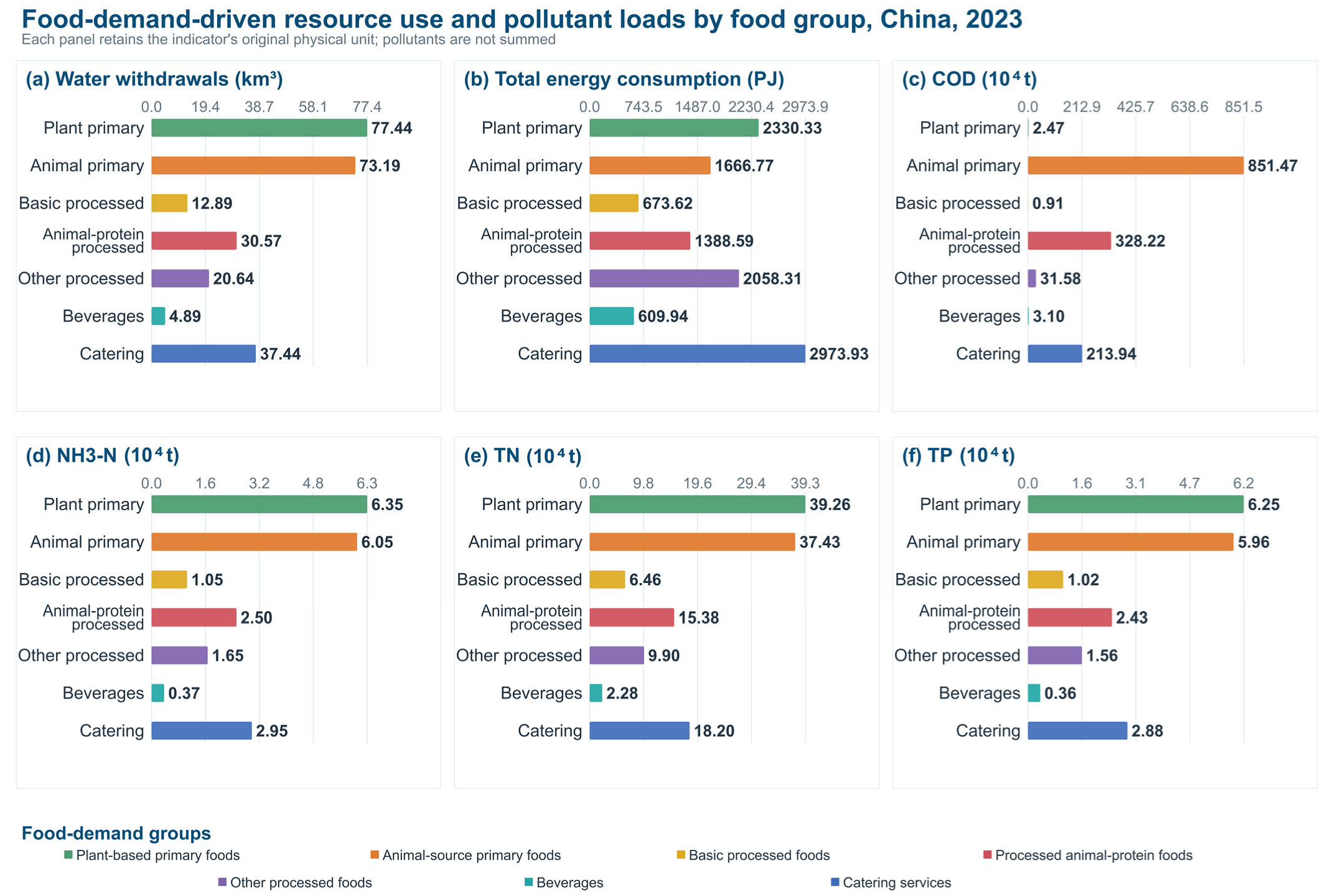
In 2023, Chinese household final demand for food induced 257 km³ of supply chain water withdrawal and 11.7 EJ of total energy consumption. The associated actual pollutant loads were 1430 × 10⁴ t of COD, 20.9 × 10⁴ t of NH₃-N, 129 × 10⁴ t of TN, and 20.5 × 10⁴ t of TP. These quantities are reported independently in indicator-specific physical units and are not summed.

Across the seven food groups, plant-based and animal-source primary foods accounted for 30.1% and 28.5% of water withdrawal. Total energy consumption was less concentrated: catering services contributed 25.4%, plant-based primary foods 19.9%, other processed foods 17.6%, and animal-source primary foods 14.2%. Animal-source primary foods accounted for 59.5% of COD loads, followed by animal-protein processed foods (22.9%) and catering services (14.9%). Plant-based primary foods led NH₃-N, TN, and TP loads (30.3–30.5%), followed by animal-source primary foods (28.9–29.1%) and catering services (14.1%).

Figure 1 thus distinguishes water-withdrawal and nutrient burdens concentrated in primary foods, COD concentrated in animal-source and animal-protein chains, and total energy consumption mobilized more broadly by catering services and processed foods through industrial and service inputs. Similar nutrient rankings do not make NH₃-N, TN, and TP interchangeable.

3.2. Production-Side Origins and Supply Chain Pathways of Environmental Pressures

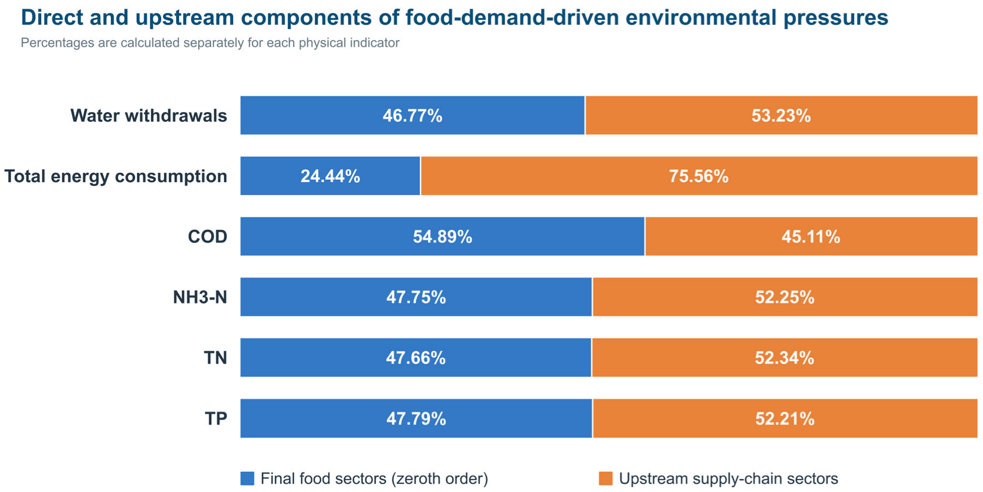
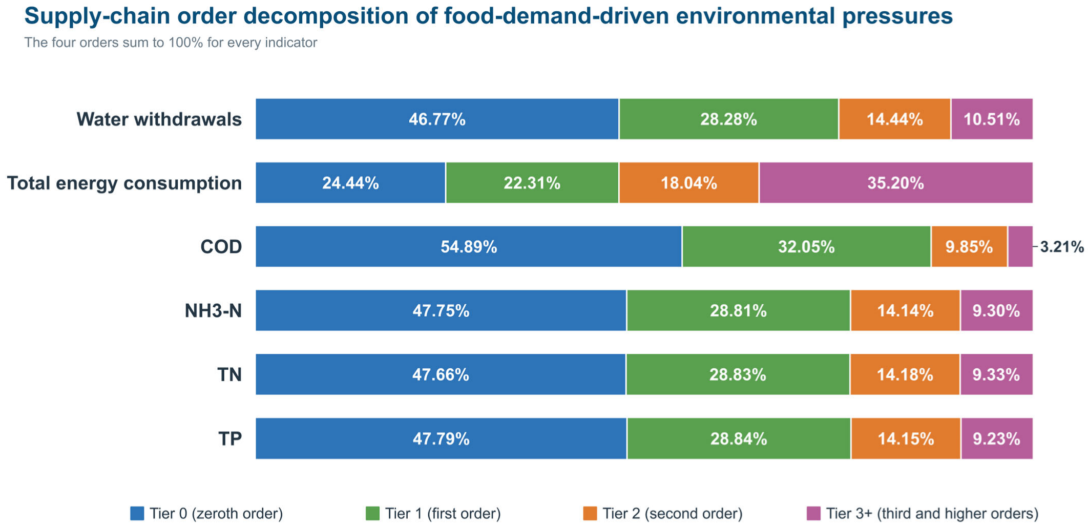
Upstream shares were 53.2% for water withdrawal, 75.6% for total energy consumption, 45.1% for COD, and 52.2–52.3% for nutrient loads (Figure 2). Water withdrawal and nutrient loads were divided approximately equally between final and upstream production; COD was shallower, while total energy consumption showed the strongest upstream dependence.

Tier decomposition confirms this contrast (Figure 3). Water-withdrawal shares declined from Tier 0 (46.8%) to Tiers 1 (28.3%), 2 (14.4%), and 3+ (10.5%). COD was shallower, with 86.9% in Tiers 0–1. Nutrient profiles were similar, with 47.7–47.8% in Tier 0 and 9.2–9.3% in Tier 3+. Total energy consumption was most deeply embedded: 24.4%, 22.3%, 18.0%, and 35.2% occurred in Tiers 0, 1, 2, and 3+, respectively.

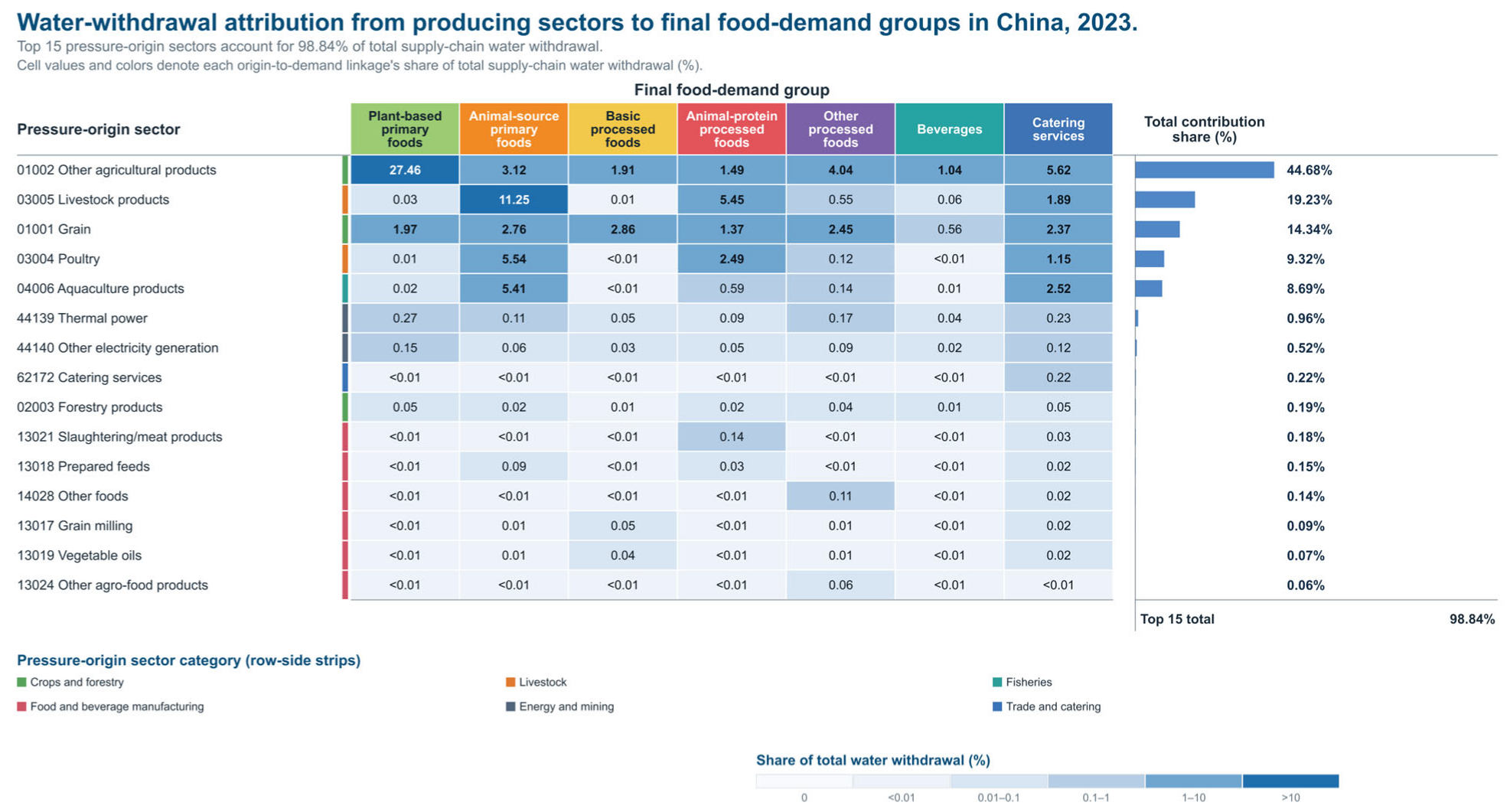
Figure 4 maps water-withdrawal attribution jointly by the producing sectors in which the pressure originated and the food sectors whose final demand induced it. Other agricultural products, livestock and other animal products, grain, poultry, and aquaculture products jointly accounted for 96.3% of total supply chain water withdrawal, showing that the production-side burden was concentrated in a small set of agricultural sectors. The prominence of the “other agricultural products” sector reflects its substantial role in agricultural production but may also be influenced by the breadth of this mixed official category. Final-demand attribution was more dispersed. Large within-sector linkages connected primary production to its own household demand, whereas the 14.5 km³ linkage from other agricultural products to catering services showed how downstream service demand induced upstream agricultural water withdrawal. The 15 producing sectors displayed in Figure 4 covered 98.8% of total water withdrawal; the 35-sector extension, covering 99.6%, is provided in Supplementary Figure S1.

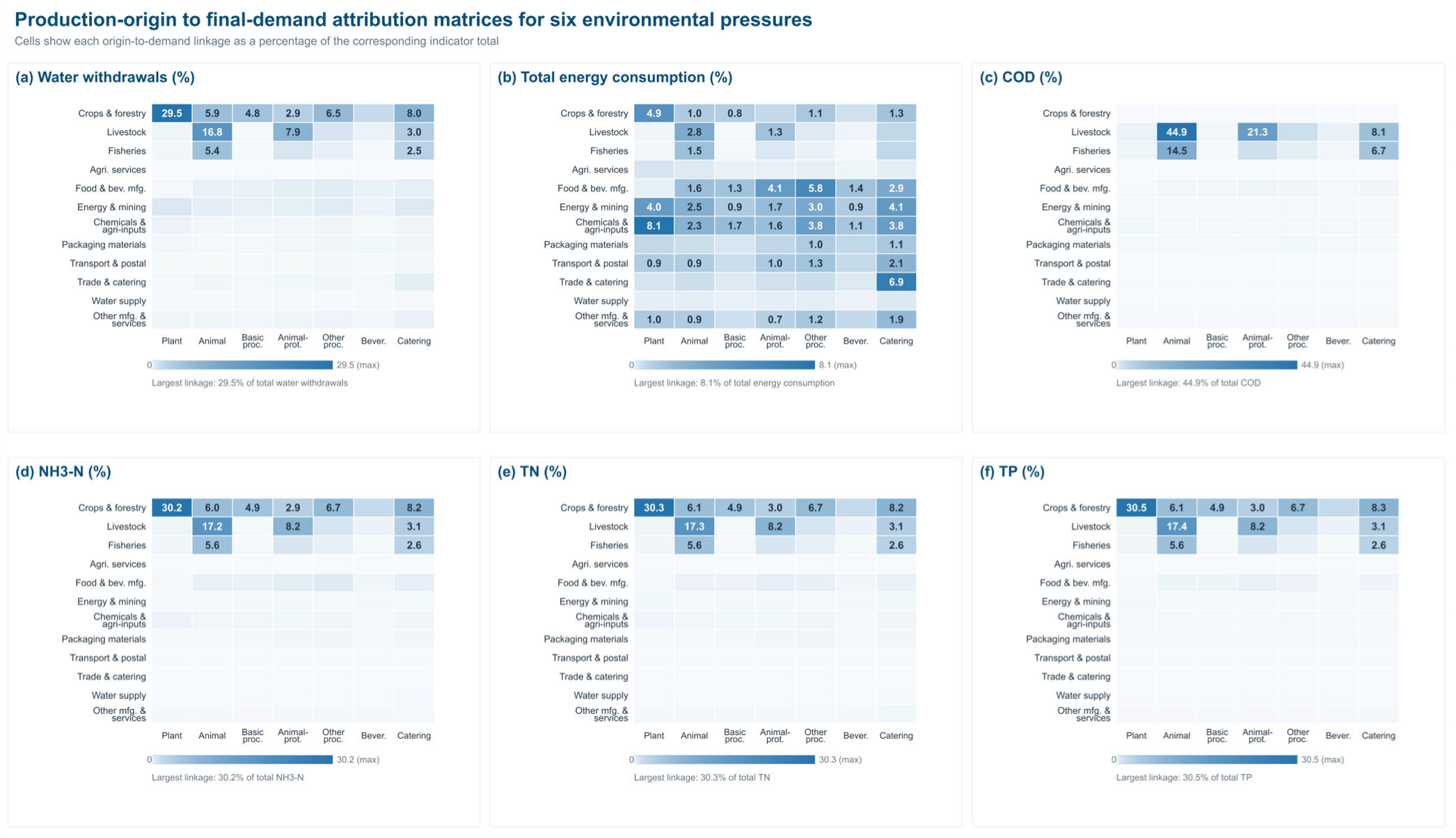
Figure 5 compares production origins with food-demand destinations. Crops and forestry supplied 59.2% of water withdrawal and 60.6–61.1% of NH₃-N, TN, and TP loads; other agricultural products were the largest demand destination (28.2–28.6%). Livestock and fisheries supplied 76.5% and 23.3% of COD, which was attributed mainly to livestock products (30.3%), slaughtering and meat products (17.9%), poultry (15.0%), catering services (14.9%), and aquaculture products (14.0%). Total energy consumption was more dispersed: chemicals and agricultural inputs supplied 22.4%, food and beverage manufacturing 17.08%, energy and mining 17.05%, and transport, storage, and postal services 7.1%; catering services were the largest demand destination (25.4%).

Attribution concentration differed sharply (

Table 3. Concentration of supply chain attribution linkages across six environmental indicators.

Indicator	Unit	Links Required for 80%	Largest Origin (Share)	Largest Demand Destination (Share)	Largest Attribution Linkage (Share)
Water withdrawal	km3	12	Crops and forestry (59.2%)	Other agricultural products (28.2%)	Crops and forestry → Other agricultural products (27.6%)
Total energy consumption	EJ	56	Chemicals and agricultural inputs (22.4%)	Catering services (25.4%)	Chemicals and agricultural inputs → Other agricultural products (7.4%)
COD	104 t	5	Livestock (76.5%)	Livestock products (30.3%)	Livestock → Livestock products (30.0%)
NH3-N	104 t	11	Crops and forestry (60.6%)	Other agricultural products (28.4%)	Crops and forestry → Other agricultural products (28.3%)
TN	104 t	11	Crops and forestry (60.8%)	Other agricultural products (28.5%)	Crops and forestry → Other agricultural products (28.4%)
TP	104 t	11	Crops and forestry (61.1%)	Other agricultural products (28.6%)	Crops and forestry → Other agricultural products (28.5%)

Note: Links are ranked by their burden within each indicator. The reported count is the minimum number of links required to reach a cumulative 80% of that indicator’s total supply chain burden. The complete pollutant attribution networks are shown in Supplementary Figure S2. The arrow (→) denotes the attribution direction from the production origin to the final-demand destination.

): covering 80% of COD required five links, compared with 11 links for each nutrient indicator, 12 for water withdrawal, and 56 for total energy consumption. Because all indicators use the same origin and destination structure, the larger energy count reflects genuinely dispersed attribution rather than unequal coverage.

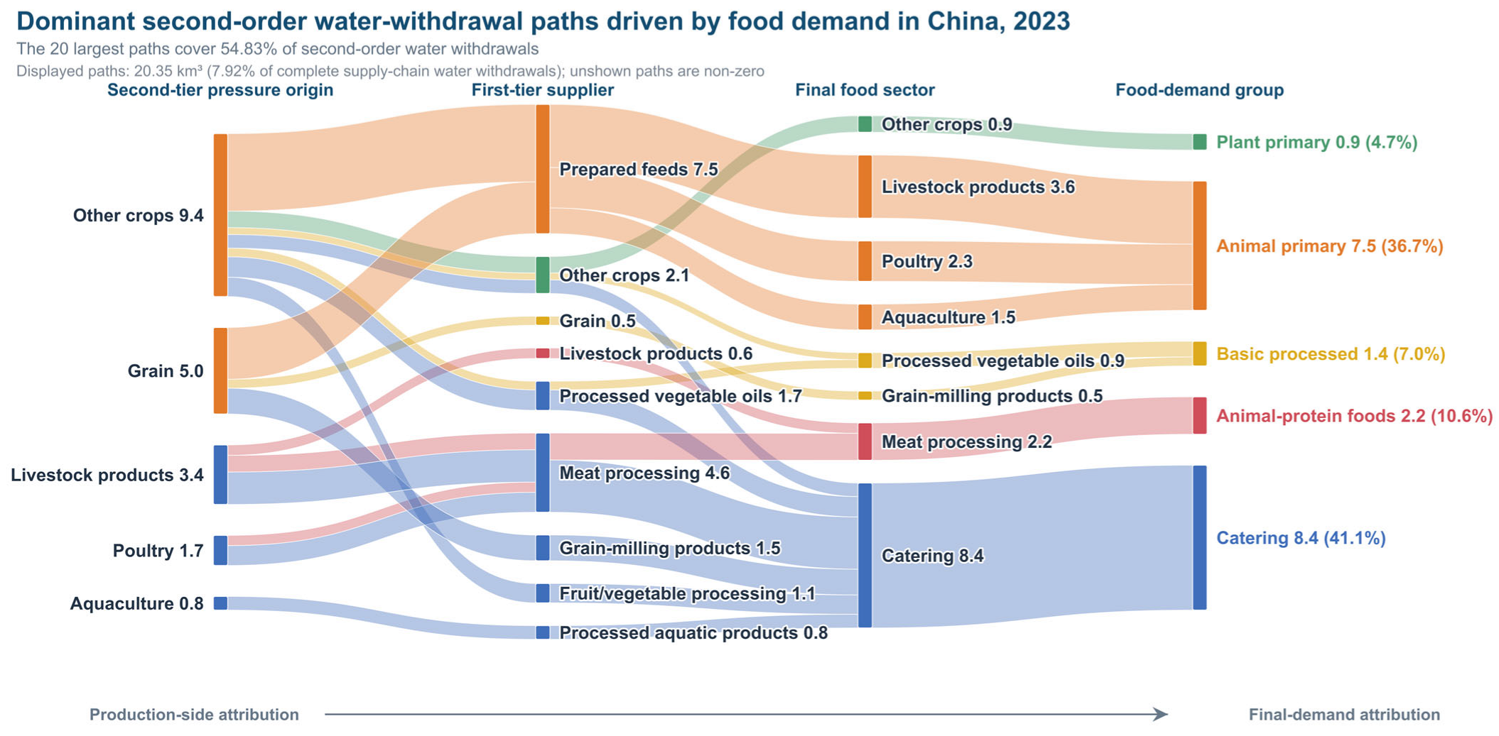
Structural path analysis identifies representative transmission pathways through two input rounds, not the complete supply chain. Figure 6 traces each path from the pressure origin through a first-tier supplier and a final food sector to the household food-demand group. The largest path—Other agricultural products → Prepared feeds → Livestock products → Animal-source primary foods—accounted for 2.18 km³ of water withdrawal, meaning that upstream withdrawal was embodied through feed and livestock production rather than physically transferred. The 20 paths represented 54.8% of second-order withdrawal and 7.9% of the full-chain total.

The 129 paths covering 90.0% of second-order withdrawal accounted for 33.4 km³ and 13.0% of full-chain withdrawal; their complete ranking is reported in Supplementary Table S1.

3.3. Recurrent Multi-Pressure Hotspots and Conditional Scenario Results

At the 80% cumulative-contribution threshold, separate core sets were constructed for water withdrawal, total energy consumption, COD, NH₃-N, TN, and TP. For each producing sector, recurrence was measured as the number of sets in which it appeared. A sector entering at least four of the six sets was classified as a recurrent multi-pressure hotspot. This operational definition identifies repeated high contributions across distinct accounts without adding or standardizing the six indicators; it does not denote statistical significance or a ranking based on a combined score.

Table 4. Producing sectors entering at least two of the six indicator-specific core sets at the 80% cumulative-contribution threshold.

Producing Sector	Sets Entered	Water	Energy	COD	NH3-N	TN	TP
Livestock and other animal products	6	19.2% ✓	3.2% ✓	51.5% ✓	19.8% ✓	19.8% ✓	19.9% ✓
Other agricultural products	5	44.7% ✓	7.5% ✓	0.0% —	45.9% ✓	46.1% ✓	46.3% ✓
Grain	5	14.3% ✓	2.4% ✓	0.0% —	14.7% ✓	14.8% ✓	14.9% ✓
Poultry	3	9.3% ✓	1.6% ✓	25.0% ✓	9.6% —	9.6% —	9.7% —
Aquaculture products	2	8.7% —	1.5% ✓	23.3% ✓	8.9% —	9.0% —	9.0% —

Note: A check mark (√) indicates inclusion in the corresponding 80% core set, whereas a dash (—) indicates non-inclusion; the percentage is the sector’s share of that indicator’s total supply-chain burden. Sectors entering at least four sets are classified as recurrent multi-pressure hotspots. Totals reported in the text are calculated from unrounded sectoral shares.

reports all sectors entering at least two core sets.

Livestock and other animal products entered all six core sets, while grain and other agricultural products each entered five; these three sectors were therefore identified as recurrent multi-pressure hotspots. Poultry entered three sets, and aquaculture products entered two. Together, the three recurrent hotspots contributed 78.3% of water withdrawal, 13.1% of total energy consumption, 51.5% of COD, 80.4% of NH₃-N, 80.7% of TN, and 81.1% of TP. Their lower joint contribution to COD reflects the pollutant mapping: among these three sectors, livestock and other animal products accounted for the mapped COD burden, whereas grain and other agricultural products dominated the three nutrient accounts.

Table 5. Conditional results of a 20% reduction in direct environmental intensities for recurrent multi-pressure hotspots.

Indicator	Unit	Absolute Reduction	Total Burden Reduction (%)	Post-Scenario Burden
Water withdrawal	km3	40.2	15.7	217
Total energy consumption	EJ	0.306	2.6	11.4
COD	104 t	147	10.3	1280
NH3-N	104 t	3.36	16.1	17.6
TN	104 t	20.8	16.1	108
TP	104 t	3.32	16.2	17.1

Note: Absolute reductions must not be added across indicators because the physical units differ. Displayed absolute values may not close exactly to the rounded baseline totals because calculations use unrounded values.

presents the intermediate illustrative scenario (20%) in which the direct environmental intensity coefficients for water withdrawal, total energy consumption, COD, NH₃-N, TN, and TP in the three recurrent hotspots were each reduced by 20%, while household final demand, the technical-coefficient matrix A, and non-target-sector intensities remained fixed. The resulting changes are conditional reductions under the assumed hotspot-sector intensity improvement rather than observed or forecast changes.

Under the 20% scenario, water withdrawal decreased by 40.2 km³ (15.7%) and total energy consumption by 0.306 EJ (2.6%). COD decreased by 147 × 10⁴ t (10.3%), while NH₃-N decreased by 3.36 × 10⁴ t, TN by 20.8 × 10⁴ t, and TP by 3.32 × 10⁴ t, corresponding to reductions of 16.1%, 16.1%, and 16.2%. The post-scenario burdens were 217 km³ of water withdrawal, 11.4 EJ of total energy consumption, 1280 × 10⁴ t of COD, 17.6 × 10⁴ t of NH₃-N, 108 × 10⁴ t of TN, and 17.1 × 10⁴ t of TP.

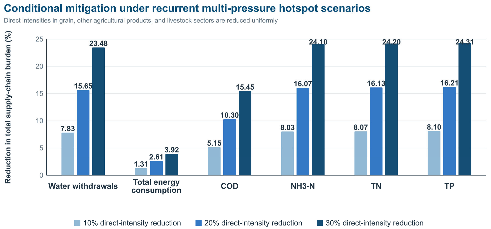
Figure 7 shows a linear response to the three conditional intensity settings. At a 10% direct-intensity reduction, total supply chain burdens declined by 7.8% for water withdrawal, 1.3% for total energy consumption, 5.2% for COD, and 8.0–8.1% for NH₃-N, TN, and TP. At a 30% reduction, the corresponding decreases were 23.5%, 3.9%, 15.5%, and 24.1–24.3%. Across all scenarios, the nutrient indicators exhibited the largest proportional reductions, while total energy consumption exhibited the smallest. This ordering follows directly from the baseline shares of the selected sectors and does not imply that real policy effects would scale linearly.

Table 6. Sensitivity of six-indicator core sets and recurrent hotspot identification to alternative cumulative-contribution thresholds.

Threshold	Water	Energy	COD	NH3-N	TN	TP	Recurrent Hotspots
70%	3	20	2	3	3	3	3
80%	4	30	3	3	3	3	3
90%	5	49	3	5	4	4	5

Note: For each indicator, the core-set size is the minimum number of sectors required for the ranked cumulative contribution to reach the stated threshold.

compares cumulative thresholds of 70%, 80%, and 90%. The water-withdrawal core set expanded from three to five sectors, and the total-energy-consumption core set from 20 to 49 sectors. The COD core set contained two sectors at 70% and three at both 80% and 90%; the NH₃-N set expanded from three to five, while the TN and TP sets expanded from three to four. The recurrent-hotspot set contained three sectors at both 70% and 80% and five at 90%. This expansion reflects broader cumulative coverage rather than a change in the underlying burden distribution.

Grain, other agricultural products, and livestock and other animal products remained hotspots at all thresholds; poultry and aquaculture products entered only at 90%.

3.4. Boundary Sensitivity Results

Excluding the mixed “other agricultural products” sector from the household food final-demand boundary reduced baseline food final demand by 18.8%. Relative to the baseline, supply chain water withdrawal declined by 28.2%, total energy consumption by 18.5%, COD by 0.16%, and NH₃-N, TN, and TP by 28.4%, 28.5%, and 28.6%, respectively. This boundary, therefore, materially affects the estimated water withdrawal and nutrient-load totals, while COD is comparatively insensitive to this boundary choice. In the service-sector pollution extension, including the estimated tertiary-industry share of domestic-source loads increased food-demand-induced COD, NH₃-N, TN, and TP by 1.1%, 6.7%, 1.9%, and 0.9%, respectively. The ordering of the seven food-demand groups remained unchanged for all four pollutants. Thus, the baseline pollution profile is relatively stable to the service-sector boundary, although NH₃-N is the most responsive of the four pollutant accounts.

4. Discussion

Three findings organize the discussion: food categories differ in their profiles of water withdrawal, total energy consumption, organic pollution, and nutrient pollution; water withdrawal and pollutant loads are concentrated in fewer, shallower agricultural links than total energy consumption; and recurrent agricultural hotspots offer substantial conditional mitigation potential for water withdrawal and nutrient loads but limited energy mitigation.

4.1. Water Quantity and Actual Pollutant Loads Lead to Divergent Priorities Across Food Sectors

Water withdrawal measures abstraction, whereas COD, NH₃-N, TN, and TP measure pollutant mass; they are neither alternative estimates nor additive components of a single burden. Separate reporting links irrigation and process-water efficiency to water withdrawal and source control, nutrient and manure management, and wastewater treatment to pollutant loads.

The results show that these priorities diverge across food chains. Plant-based primary foods produced the largest water-withdrawal burden and 30.3–30.5% of NH₃-N, TN, and TP, whereas animal-source primary foods generated 59.5% of COD and 28.9–29.1% of the nutrient loads. The production-origin results sharpen this distinction: crops and forestry accounted for 60.6–61.1% of the three nutrient pollutants, while livestock production accounted for 76.5% of COD. Global food-system evidence likewise identifies nutrient pollution as a major agricultural footprint [3], and livestock research traces nitrogen and phosphorus pressures through feed, manure, and production chains [13,14,15]. These patterns imply that crop-chain water saving cannot substitute for organic pollution control in livestock chains, and neither intervention substitutes for nitrogen and phosphorus management.

The NH₃-N and TN accounts connect to, but are narrower than, nitrogen footprint research. Such models cover multiple reactive nitrogen species across production, consumption, and waste [11,12], while NutrIO and national studies include indirect industrial inputs and broader food-system losses [10,16,17]. Here, only water pollution loads reported as NH₃-N and TN are traced; atmospheric emissions, soil accumulation, product nitrogen, denitrification, and cross-media transfers remain outside the boundary.

Separating the four pollutants prevents one pathway from masking another. COD originated mainly in livestock and fisheries and was attributed to demand for livestock products, meat processing products, poultry, catering services, and aquaculture products. NH₃-N and TN reflect crop and fertilizer releases together with feed and livestock nutrient losses; crops and forestry supplied 60.6% and 60.8% and livestock 29.3% and 29.4%. TP requires phosphorus-specific interpretation: crops and forestry supplied 61.1% and livestock 29.6%, linking control to fertilizer efficiency, runoff prevention, manure recovery, and phosphorus removal. These annual sector-level loads identify pollutant-load attribution, not pollutant fate or local ecological damage.

4.2. Environmental Pressures Exhibit Different Degrees of Supply Chain Embedding

Upstream sectors generated about half of water withdrawal and nutrient loads but 75.6% of total energy consumption. COD had a shallower supply chain profile, with 86.9% in Tiers 0–1; Tier 3+ contributed 35.2% of total energy consumption versus 10.5% of water withdrawal and 3.2–9.3% of pollutant loads. This pattern accords with consumption-based EEIO/MRIO attribution [20,21,22] and evidence on indirect food-chain burdens in China [8].

The total-energy profile reflects the cumulative industrial inputs required to supply food rather than energy use only within agriculture or food processing. Chemicals and agricultural inputs were the largest production origin (22.4%), followed by food and beverage manufacturing (17.08%) and energy and mining (17.05%); transport, storage, and postal services added 7.1%. Catering services induced 25.4% of total energy consumption, connecting final demand for catering services with these dispersed suppliers. This pattern is consistent with the EEIO principle that final demand mobilizes pressures through remote industrial inputs [20,21,22] and with evidence on the intermediary roles of energy-extraction, energy-conversion, and chemical sectors in WEF networks [23,24]. NutrIO similarly shows that excluding chemical and fossil-fuel inputs understates the full-chain nitrogen inputs associated with food consumption [10]. The contrast with COD and nutrient pollution is therefore structural: energy accumulates over numerous production rounds, whereas pollutant loads remain more closely tied to biological production and waste-generating activities.

Link concentration reinforces the contrast: 80% coverage required 5 links for COD, 11 for each nutrient, and 12 for water withdrawal, but 56 for total energy consumption. Water-withdrawal and pollution policy can focus on major agricultural and food links; energy policy must span chemicals, power, fuels, transport, storage, and services [25,44].

This structural difference cautions against composite WEF scores. Although normalization and weighting yield concise rankings, results can depend on indicator choice and weighting [29] and can conceal the contrast between concentrated water/pollution networks and dispersed energy networks. Indicator-specific accounts instead distinguish recurrent multi-pressure nodes from pressure-specific upstream nodes, showing whether governance should be focused or distributed.

4.3. Pressure Origins, Structural Paths, and Final-Demand Attribution Require Joint Interpretation

Production-based attribution indicates that water withdrawal induced by final food demand is highly concentrated in five pressure-origin sectors: other agricultural products, livestock and other animal products, grain, poultry, and aquaculture products. From a final-demand attribution perspective, however, the associated burdens are distributed across primary agricultural products, processed foods, and catering services. The largest attribution linkages include both within-sector relationships, in which primary sectors supply their own final demand, and cross-sector relationships, particularly the supply of other agricultural products to demand for catering services. Supplementary Figure S3 also reveals pronounced directional net-burden relationships from other agricultural products to catering services and from livestock and other animal products to final demand for slaughtering and meat products. Thus, concentration at the pressure-origin end identifies where burdens occur, whereas final-demand attribution identifies the downstream demand that induces upstream production through intersectoral purchasing relationships.

Second-order structural paths make this upstream demand transmission explicit. Other agricultural products, grain, and livestock and other animal products are the principal pressure-origin sectors along second-order water-withdrawal paths, whereas feed processing, slaughtering and meat processing, and grain milling serve as important first-tier connecting sectors. Among final-demand categories, catering services account for the largest share of second-order water-withdrawal attribution. This structure is consistent with international evidence that livestock supply chains transmit water, land, and nitrogen pressures through feed production [7,13,32] and with the argument that hybrid input-output models should jointly represent physical agricultural flows and monetary interindustry relationships [27]. Households do not generally purchase feed or other intermediate agricultural inputs directly; instead, final demand for livestock products, processed meat, and catering services embodies these upstream inputs. Consequently, neither an assessment restricted to final food-demand sectors nor one focused only on pressure-origin sectors can fully represent the distribution and drivers of supply chain water withdrawal.

The 129 paths covered 90.0% of second-order withdrawal but only 13.0% of the full-chain total. They reveal two rounds of transactions, not burdens in Tier 0, Tier 1, or Tier 3+. Reporting both coverage measures preserves the chain interpretation of structural path decomposition [30] without overstating it as complete consumption-based attribution [22].

4.4. Recurrent Multi-Pressure Hotspots Reveal the Potential and Limits of Synergistic Governance

Livestock and other animal products, grain, and other agricultural products were recurrent hotspots because each entered at least four indicator-specific 80% core sets. This operational screen is neither a composite index, a significance test, nor an ecological-risk ranking; it does not imply physical equivalence or identify the sole causal sources. Their joint shares were high for water withdrawal (78.3%) and nutrients (over 80%) but lower for COD (51.5%) and total energy consumption (13.1%); recurrence therefore identifies coordination opportunities without replacing pressure-specific priorities.

The conditional mitigation results make this asymmetry explicit. A uniform 20% reduction in the six indicator-specific direct environmental intensities of the three recurrent hotspots reduced water withdrawal by 15.7% and NH₃-N, TN, and TP by 16.1–16.2%, but COD by 10.3% and total energy consumption by only 2.6%. The small energy response is explained by the baseline structure: the three agricultural hotspots supplied only 13.1% of the energy burden, whereas chemicals and agricultural inputs, food and beverage manufacturing, energy and mining, transport, storage, and other services supplied substantial additional shares. Because the simulations hold household final demand and interindustry coefficients fixed, leave non-target-sector intensities unchanged, and assume simultaneous improvement across all selected sectors, they indicate the relative mitigation leverage of hotspot-sector intensity improvements within the modeled structure. They do not predict real-world reductions, establish policy effectiveness, or demonstrate technological feasibility. Recurrent hotspots provide a starting point for coordinated intervention, but COD control must also cover poultry, aquaculture, slaughtering, processing, and other organic waste sources, while energy policy must reach the wider industrial network.

The same three sectors remained hotspots at cumulative thresholds of 70%, 80%, and 90%; poultry and aquaculture products entered the hotspot set only at the 90% threshold. The 80% baseline follows cumulative-contribution screening [38], not a significance test or fixed Pareto rule. Stability identifies robust priorities, while the 90% set shows the sectors needed for broader coverage.

4.5. Implications for Water–Energy–Food Governance Across Food Supply Chains

The results support governance differentiated by pressure type and supply chain position. Water-saving measures should focus on irrigation efficiency, process-water reuse, and reduction of conveyance losses in crop and other agricultural production. COD control should prioritize manure and organic waste management in livestock and poultry production, organic wastewater from aquaculture, and treatment at slaughtering, food-processing, and catering facilities. NH₃-N and TN management should combine fertilizer optimization, crop nutrient-use efficiency, field-loss prevention, feed management, manure recovery, and monitoring of nitrogen discharges. TP control requires phosphorus fertilizer management, erosion and runoff prevention, manure phosphorus recovery, and treatment of phosphorus-rich effluents. These pollutant-specific measures should be complemented by energy-efficiency improvements across chemicals, power, fuels, food manufacturing, transport, and storage.

Feed processing, slaughtering and meat processing, grain milling, and catering services provide practical governance interfaces between upstream production and final demand. Their procurement standards, supplier-selection practices, product portfolios, and traceability systems can influence upstream production even when they are not the largest direct water users or pollutant emitters. Processing and catering enterprises can therefore transmit demand-side environmental requirements through supplier disclosure, sustainable procurement, raw material traceability, and food loss and waste management. Households can complement these measures through food choices, responses to environmental information, and waste reduction, while public authorities can use green public procurement and disclosure requirements. Dietary change can alter supply chain water requirements [6], and demand for animal-source protein can mobilize land and water resources through international feed trade [7]. International scenario and producer-level studies indicate that demand-side dietary change and producer-side improvements are complementary intervention domains [2,4]. However, because this study does not simulate dietary substitution, prices, nutrition, or distributional effects, it cannot prescribe quantitative reductions in particular food categories.

Energy governance requires broader coverage: chemicals and agricultural inputs, food and beverage manufacturing, and energy and mining supplied 56.5% of total energy consumption, with transport, storage, and postal services adding 7.1%. These sectors represent fertilizer and chemical inputs, power and heat, fuels, manufacturing, and logistics; cold chains are not separately identified. The hotspots’ 13.1% share of total energy consumption explains the 2.6% mitigation response and confirms the need for energy-specific industrial action [8,33,34].

4.6. Limitations and Future Research

First, the sectoral resolution of the environmental accounts imposes an important limitation on the analysis. National statistics provide authoritative aggregate totals for water withdrawal, energy consumption, and pollutant discharges in 2023, but their industrial classifications do not align perfectly with those of the 211-sector input-output table. Some aggregate environmental totals, therefore, had to be disaggregated using sectoral concordance relationships and output shares. Consequently, the detailed sectoral estimates combine official aggregate statistics with concordance and allocation assumptions; they should not be interpreted as independently observed environmental accounts for all 211 sectors. Because the water account is withdrawal-based, it cannot directly characterize consumptive blue water use or evapotranspiration-related water consumption; the reported water results represent abstraction pressure, not a blue water footprint. The delineation of final food demand sectors is also constrained by the available input–output classification. Catering services combine food ingredients with energy and other service inputs, whereas some processed food and distribution activities extend across multiple input-output sectors. The 21 final food demand sectors selected in this study, therefore, do not correspond exactly to household dietary intake as defined in nutritional assessments. In addition, the official sector classified as “other agricultural products” combines food commodities with certain non-food cash crops and related agricultural products. Its high estimated contribution should be interpreted as reflecting both its substantive role in agricultural supply and potential within-sector aggregation heterogeneity; it does not imply that every constituent commodity has the same burden profile. Although the economic and environmental accounts were harmonized as closely as possible to the 2023 accounting year, monetary input–output relationships remain affected by differences in sectoral prices and product values. A monetary unit of output, therefore, does not represent an equivalent quantity of physical production across agriculture, manufacturing, processing, and service sectors. Future research could use crop-water-use and evapotranspiration data in spatial agricultural models to assess green-water consumption, alongside physical supply-use tables and facility-level pollution data for hybrid physical–monetary input-output analysis [27].

Second, the national single-region model assigns burdens to sectors, not provinces or basins, and cannot resolve regional water availability, hydrology, energy mixes, or receiving-water conditions. Pollutant accounts omit fate, transport, retention, removal, seasonality, ecological sensitivity, and within-sector technological variation; results therefore indicate pollutant-load attribution rather than local concentrations or risk. NH₃-N and TN also omit other reactive nitrogen species and pathways. Provincial MRIO, basin data, spatial inventories, and fate models could address these gaps.

Third, the competitive input-output framework assumes product homogeneity and fixed technical coefficients and treats imported products according to the domestic technology assumption. It therefore cannot distinguish between environmental pressures arising from domestic production and those embodied in imported products. The results should be interpreted as pressures attributed to China’s final food demand under the 2023 competitive input-output framework, rather than as a complete inventory of pressures physically occurring within China. In temporal terms, the 2023 analysis is a static snapshot. It cannot reveal trends associated with technological improvement, dietary transition, policy-induced change, climate variability, or structural economic change. The direct environmental-intensity reduction scenarios hold final demand and interindustry input structures constant and therefore estimate conditional mitigation potential within the fixed model structure; they do not predict future policy effects, implementation costs, macroeconomic adjustment, or behavioral responses. Future research could use multi-year dynamic input-output models to track changes in technology, diets, policy, climate conditions, and economic structure, while non-competitive or multiregional models could distinguish domestic production from imported supply chain sources.

Finally, this study employs point estimates of direct environmental intensities within a deterministic accounting framework and does not systematically propagate uncertainties arising from source statistics, sectoral concordance, allocation procedures, or model parameters. The comparison of cumulative contribution thresholds of 70%, 80%, and 90% evaluates the sensitivity of hotspot membership to the screening criterion, but it does not constitute an uncertainty analysis of the underlying environmental accounts or model coefficients. The detailed sectoral disaggregation of the energy account depends heavily on concordances between industry-level energy statistics and input-output sectors. The energy estimates may therefore be particularly sensitive to sectoral mapping and output-based allocation assumptions, although the relative magnitude of uncertainty across environmental accounts was not quantified in this study. Future studies could further validate the allocated 211-sector estimates using detailed industry energy-balance data and facility- or enterprise-level energy-use records. Probability distributions could also be specified for water, energy, and pollutant-intensity coefficients, and Monte Carlo simulation could be used to estimate uncertainty intervals for aggregate burdens, rank probabilities for individual sectors, and probabilities of hotspot membership.

5. Conclusions

Using a 211-sector EEIO model and 2023 household food demand, this study quantified six separate environmental pressures and traced their food category profiles, production origins, supply chain tiers and paths, recurrent hotspots, and conditional mitigation.

(1)

Household food demand induced 257 km³ of water withdrawal, 11.7 EJ of total energy consumption, and the following pollutant loads: COD (1430 × 10⁴ t), NH₃-N (20.9 × 10⁴ t), TN (129 × 10⁴ t), and TP (20.5 × 10⁴ t). Upstream sectors accounted for 53.2% of water withdrawal, 75.6% of total energy consumption, 45.1% of COD, and 52.2–52.3% of the nutrient loads. Total energy consumption was therefore substantially more deeply embedded than water withdrawal and actual pollutant loads.

(2)

Environmental priorities differed by food category and production origin. Plant-based primary foods accounted for the largest shares of water withdrawal and NH3-N, TN, and TP, while animal-source primary foods dominated COD. Crops and forestry supplied 60.6–61.1% of nutrient loads, livestock supplied 76.5% of COD, and chemicals and agricultural inputs were the largest energy origin at 22.4%. Energy attribution was distributed across far more links and upstream tiers than water-withdrawal or pollutant-load attribution.

(3)

At the 80% threshold, grain, other agricultural products, and livestock and other animal products were recurrent multi-pressure hotspots. A conditional 20% reduction in their direct intensities lowered water withdrawal by 15.7%, COD by 10.3%, NH₃-N, TN, and TP by 16.1–16.2%, and total energy consumption by 2.6%. The comparatively small energy reduction reflects the hotspots’ 13.1% baseline energy share and confirms that coordinated agricultural intervention must be supplemented by energy-specific action in chemicals, power, fuels, manufacturing, transport, storage, and service sectors.

Governance should therefore combine water saving, energy efficiency, COD control, nitrogen and phosphorus management, manure and organic waste recovery, and wastewater treatment through pressure- and sector-specific measures. Within the national 2023 boundary, the results describe supply chain attribution and conditional mitigation potential, not local risk, temporal trends, or causal policy effects.