A Hydraulically Informed ANN Surrogate Framework for Nonlinear Open-Channel Flow Analysis

Abstract

Open-channel hydraulic analysis often requires repeated solution of implicit nonlinear equations and numerical integration of gradually varied flow (GVF), which can become computationally demanding in inverse, optimization, and sensitivity applications. This study develops a hydraulically informed artificial neural network (ANN) surrogate framework comprising ten independently trained models for normal and critical depths, alternative and conjugate depths, GVF-related water-surface behavior, and profile-based discharge inference. Hydraulic information is introduced through physically meaningful, and where appropriate dimensionless, variables and reference solutions derived from established governing equations or numerical hydraulic models, while ANN optimization remains data driven. Equation-generated test sets quantified surrogate fidelity, whereas HEC-RAS comparisons were treated as numerical hydraulic cross-verification rather than independent physical validation. The forward surrogates reproduced their reference mappings with high accuracy within the represented domains. Benchmarking against Random Forest, support vector regression, and Gaussian Process Regression for Models 1, 5, and 7 showed no universal algorithmic superiority; however, ANN provided a favorable trade-off among accuracy, relative-error robustness, compactness, and repeated-inference efficiency. For Model 7, ANN inference was approximately 249 times faster than conventional GVF calculation, with development cost recovered after about 1.03 × 10⁵ evaluations. Model 9 inferred discharge with a 4.75% error in the profile-based test. Observation-based assessment using 16 historical Missouri River stage–discharge events showed that direct HEC-RAS inversion yielded a MAPE of 44.71%, whereas observation-only ANN and hybrid HEC-RAS-ANN discrepancy correction reduced MAPE to 10.25% and 9.83%, respectively. The framework is therefore a computational complement to established hydraulic equations and numerical models, with broader field validation and explicit uncertainty treatment required for general deployment.

1. Introduction

Open-channel flow analysis is fundamental to the planning, design, and operation of rivers, irrigation and drainage systems, culverts, spillways, and hydraulic-control structures. A typical hydraulic analysis requires the determination of several interconnected variables, including normal depth, critical depth, alternative and conjugate depths, and gradually varied flow (GVF) profiles. These quantities represent distinct hydraulic mechanisms: normal depth reflects the equilibrium between gravitational driving forces and boundary resistance; critical depth defines the inertia–gravity transition between subcritical and supercritical flow; alternative depths satisfy specific-energy equivalence; conjugate depths are governed by momentum conservation; and GVF describes the longitudinal adjustment of the free surface under steady nonuniform flow [1,2,3,4,5]. For non-rectangular cross-sections, several of the corresponding governing equations are nonlinear and implicit with respect to water depth and therefore require iterative numerical solution. GVF calculations introduce an additional computational requirement because the governing differential equation must be integrated spatially along the channel reach. Although conventional numerical procedures are well established and reliable, their repeated execution may become computationally demanding when embedded in parametric studies, optimization procedures, sensitivity analyses, repeated design calculations, and inverse hydraulic problems.

These computational considerations have motivated the use of artificial neural networks (ANNs) and other machine-learning approaches as surrogate models for hydraulic calculations. Earlier ANN applications demonstrated their capability to approximate nonlinear relationships associated with friction coefficients and flow resistance in open channels [6,7,8], hydraulic characteristics of irregular channels [9], and combined and compound-channel flows [10,11]. ANN modeling was subsequently extended to complex flow at open-channel junctions [12], vegetation-affected channels [13], and flow characteristics through channel bends [14]. Machine-learning approaches have also been applied specifically to GVF-related problems, including estimation of GVF profile lengths [15] and prediction of water-surface profiles in nonprismatic compound channels [16]. Collectively, these studies established that appropriately trained data-driven models can reproduce complex hydraulic input–output relationships with good accuracy. More recent work has further emphasized the incorporation of prior physical information into neural-network formulations as a means of improving generalization and maintaining consistency with known hydraulic behavior [17].

Recent developments have moved hydraulic machine learning beyond conventional standalone ANN regression toward physics-informed and structure-aware approaches. Physics-informed neural networks (PINNs) incorporate governing equations, boundary conditions, or associated residuals directly into the learning process. PINNs have recently been applied to two-dimensional shallow-water equations without requiring conventional labeled training data [18], as well as to one-dimensional steady open-channel flows for water-surface prediction and roughness estimation under different flow regimes and complex bed configurations [19]. Further developments have addressed shallow-water systems with explicit representation of bed topography [20] and one-dimensional unsteady riverine flows governed by the shallow-water equations [21]. These studies demonstrate the potential of physics-informed learning to establish a stronger connection between machine-learning predictions and governing hydraulic principles.

Graph neural networks (GNNs) constitute another rapidly developing direction because the connectivity among hydraulic elements or computational nodes can be represented explicitly within the learning architecture. A GNN-based surrogate has recently been developed for real-time hydraulic prediction in urban drainage networks [22], while multi-scale hydraulic GNNs have been applied to spatiotemporal flood propagation over irregular computational domains and previously unseen topographies [23]. Attention-based architectures have also entered hydraulic modeling. In particular, a Transformer-based deep-learning model has been developed for rapid sequential forecasting of flood inundation maps under dam-break scenarios [24]. These developments illustrate the broader transition toward AI models capable of representing not only nonlinear hydraulic relationships but also the spatial, temporal, and physical structure of water systems.

Artificial intelligence has simultaneously become increasingly important in flood forecasting, susceptibility assessment, and flood-risk management. Recent deep-learning systems have demonstrated the capability to predict extreme floods at large spatial scales, including in ungauged watersheds [25]. Tree-based and ensemble-learning techniques have also become prominent because of their ability to represent nonlinear interactions among hydrological, meteorological, topographic, and geomorphological predictors. Recent flood-susceptibility studies have demonstrated the potential of stacking ensembles that combine complementary machine-learning algorithms [26]. Other recent investigations have compared Random Forest, AdaBoost, XGBoost, LightGBM, and CatBoost for rapid flood mapping and assessment, showing that predictive accuracy and computational efficiency are generally problem-dependent rather than universally dominated by a single algorithm [27]. These developments highlight the growing role of ensemble machine learning in flood prediction and risk-informed water-resources management.

Generative artificial intelligence represents an additional emerging direction in hydrology and water-resources engineering. Unlike conventional predictive machine-learning models, large language models (LLMs) can support knowledge synthesis, multimodal information processing, model interpretation, workflow guidance, and interaction with complex hydrological information. WaterGPT introduced a hydrology-oriented LLM framework designed to support domain-specific reasoning, multimodal analysis, and water-resources decision support [28]. More recently, HydroCraft integrated an LLM-based agent within a hydrological-modeling environment to facilitate model setup, execution, and user interaction [29]. Although such Generative AI systems are not direct alternatives to deterministic hydraulic solvers or numerical surrogate models, they illustrate the broader evolution toward increasingly automated and interactive AI-assisted water-resources modeling environments.

Despite these substantial advances in conventional machine learning, physics-informed learning, graph-based modeling, attention-based architectures, ensemble methods, and Generative AI, most existing studies remain focused on individual prediction tasks, particular hydraulic processes, or broader hydrological and flood-risk applications. Comparatively limited attention has been given to developing an application-oriented surrogate framework that follows the sequence of classical open-channel hydraulic calculations, beginning with uniform- and critical-flow states, progressing through energy- and momentum-controlled local transitions, extending to spatial GVF behavior, and finally supporting inverse estimation of discharge from water-surface information. This distinction is important because practical open-channel analysis commonly requires several of these calculations to be performed sequentially rather than as isolated prediction tasks.

The present study addresses this gap by developing a hydraulically informed ANN surrogate framework that coordinates several fundamental nonlinear open-channel flow calculations within a common computational workflow. The novelty does not reside in the underlying hydraulic relationships, which are well established, nor in the isolated application of ANN regression to individual hydraulic variables. Rather, the contribution is framework-level: established hydraulic processes are formulated as compatible surrogate mappings spanning normal and critical flow, energy- and momentum-controlled transition depths, gradually varied flow (GVF), spatial water-surface-profile prediction, and inverse discharge estimation. This coordinated formulation converts implicit or numerically integrated hydraulic relationships into rapidly evaluated mappings that can be repeatedly embedded in higher-level inverse, sensitivity, optimization, and operational-analysis procedures. Model 9 illustrates this extension by using water-surface-profile information to infer discharge, while Model 10 further demonstrates an observation-informed natural-river application in which a numerical hydraulic baseline is combined with site-specific stage–discharge information through discrepancy correction. Thus, the principal contribution is the organization of established hydraulic knowledge into a coordinated family of computationally efficient surrogate operators supporting both forward and inverse open-channel hydraulic analysis, rather than the introduction of new hydraulic equations or a fundamentally new neural-network methodology.

In this study, the term hydraulically informed ANN refers to a supervised surrogate whose problem formulation and training information are guided by established hydraulic principles, rather than to a physics-informed neural network (PINN). Hydraulic knowledge enters through the definition of the individual prediction problems, the selection of physically meaningful and, where appropriate, dimensionless input and output variables, the specification of hydraulically relevant applicability domains, and the generation of reference targets from governing equations or numerical hydraulic models. The ANN optimization itself remains data driven; governing-equation residuals, conservation constraints, and physics-based penalty terms are not embedded in the loss function. Consequently, the proposed models should not be interpreted as PINNs and do not inherently guarantee exact conservation, monotonicity, positivity, or physically admissible extrapolation beyond the domains represented during model development. The term hydraulically informed therefore denotes physics-guided surrogate formulation and reference-data construction rather than physics-constrained network optimization.

The framework encompasses normal- and critical-depth prediction for trapezoidal and circular sections, alternative- and conjugate-depth prediction for trapezoidal channels, and GVF-related mappings for mild- and steep-slope reaches. It is subsequently extended from forward prediction to profile-based inverse discharge estimation and to an observation-informed natural-river application incorporating site-specific hydraulic information, HEC-RAS-generated relationships, and historical water-level observations. Predictive performance is evaluated using held-out testing datasets and statistical error measures, while comparisons with conventional hydraulic solutions and HEC-RAS provide numerical hydraulic cross-verification. Computational benchmarking quantifies the efficiency of the trained surrogates during repeated evaluation, and complementary architecture- and inverse-discharge-sensitivity analyses examine model robustness and the propagation of observational uncertainty; further details are provided in Supplementary Sections S1 and S2.

Accordingly, the primary objective is to determine whether a coordinated set of ANN surrogates can reproduce representative nonlinear open-channel hydraulic relationships with sufficient accuracy and computational efficiency to support repeated engineering calculations and inverse-analysis workflows. The assessment therefore considers not only predictive performance, but also computational benefit, hydraulic interpretability, sensitivity to observational uncertainty, and the practical limitations associated with the represented hydraulic domains. Collectively, these analyses establish the scope within which ANN-based surrogates can provide a useful computational complement to conventional open-channel hydraulic solution procedures.

2. Materials and Methods

2.1. Methodological Framework

Following the objectives defined in Section 1, the methodology was designed to develop a hydraulically informed ANN-based surrogate framework for a sequence of nonlinear open-channel flow calculations. The framework does not treat the ANN models as purely empirical input–output correlations. Instead, each model was formulated around a governing hydraulic principle and trained using variables that preserve the physical structure of the corresponding problem. The selected modeling sequence reflects the normal workflow of open-channel analysis: first, uniform-flow and critical-flow depths are determined; second, local transition depths are evaluated through energy and momentum principles; third, gradually varied flow (GVF) profiles are represented for gate-controlled mild and steep reaches; and finally, water-surface-profile information is used to support inverse discharge estimation.

Ten ANN models were therefore considered. Models 1 and 2 estimate the normal depth in trapezoidal and circular cross-sections, respectively. Models 3 and 4 estimate the critical depth in the same two cross-section types. Models 5 and 6 estimate the alternative and conjugate depths in trapezoidal channels. Models 7 and 8 represent GVF-related depth ratios for mild and steep gate-controlled reaches, respectively. Model 9 extends the framework from forward hydraulic prediction to profile-based discharge inference by predicting the longitudinal water-depth distribution upstream of a control section.

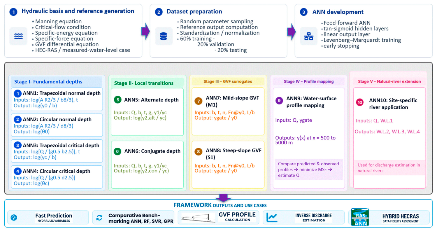
As illustrated in Figure 1, the methodological workflow integrates hydraulic-reference generation, dataset preparation, ANN development, and independent hydraulic assessment. The detailed governing formulations, input–output definitions, dataset-generation procedures, and ANN training strategy are presented in the following subsections.

The proposed framework comprises ten ANN models, organized according to their hydraulic functions and levels of application. Models 1 and 2 estimate normal depth in trapezoidal and circular cross-sections, respectively, whereas Models 3 and 4 estimate the corresponding critical depths. Models 5 and 6 address local hydraulic transitions by predicting alternative and conjugate depths based on the specific-energy and specific-force principles, respectively. Models 7 and 8 represent gradually varied flow under mild- and steep-slope conditions. Model 9 extends the framework from direct hydraulic prediction to water-surface-profile mapping and inverse discharge estimation by relating discharge and downstream-control depth to the longitudinal distribution of water depth. Finally, Model 10 extends the framework to a site-specific natural-river application, in which discharge and the downstream water level are used to predict water levels at upstream cross-sections, enabling discharge estimation through comparison with measured water levels. Thus, the ten models collectively span uniform-flow, critical-flow, local-transition, gradually varied flow, inverse-estimation, and natural-river applications. The complete methodological structure—including hydraulic-reference generation, dataset preparation, ANN development, the functions of all ten ANN models, and their principal engineering applications—is summarized in Figure 1.

2.2. Hydraulic Basis of the ANN Models

2.2.1. Normal-Depth Formulation

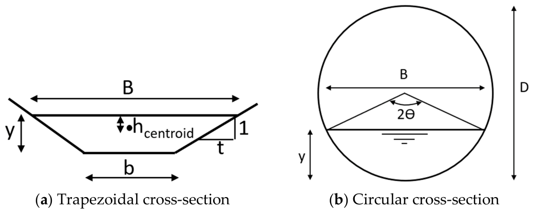
Normal depth represents the equilibrium flow depth attained when the gravitational driving force along the channel bed is balanced by boundary resistance. In the present framework, normal depth was evaluated for two commonly used cross-sectional forms: trapezoidal open channels and partially full circular conduits. The geometric definitions of these two sections and the associated variables used in the hydraulic formulations are shown in Figure 2. For the trapezoidal section, the governing geometric variables are the bed width (b), flow depth (y), side slope (t), top width (B), flow area (A), and wetted perimeter (P). For the circular section, the hydraulic geometry is described using the pipe diameter (D), flow depth (y), water-surface chord width (B), and the central angle (θ), which controls the wetted area and wetted perimeter.

Normal depth was computed from Manning’s equation, which expresses the balance between gravitational driving force, boundary resistance, and channel conveyance:

$$\mathrm{Q}=\mathrm{A}\times {\displaystyle \frac{1}{\mathrm{n}}}\times {\mathrm{R}}^{2/3}\times {\mathrm{S}}_{\mathrm{o}}^{0.5}$$

(1)

where (Q) is the discharge, (n) is Manning’s roughness coefficient, (A) is the flow area, (R) is the hydraulic radius, (P) is the wetted perimeter, and (S_o) is the bed slope. For trapezoidal sections, the hydraulic geometry was defined as:

$${\mathrm{A}}_{\mathrm{t}\mathrm{r}\mathrm{a}\mathrm{p}\mathrm{e}\mathrm{z}\mathrm{o}\mathrm{i}\mathrm{d}\mathrm{a}\mathrm{l}}=\mathrm{b}\mathrm{y}+\mathrm{t}{\mathrm{y}}^2$$

(2)

$${\mathrm{P}}_{\mathrm{t}\mathrm{r}\mathrm{a}\mathrm{p}\mathrm{e}\mathrm{z}\mathrm{o}\mathrm{i}\mathrm{d}\mathrm{a}\mathrm{l}}=\mathrm{b}+2\mathrm{y}\sqrt{1+{\mathrm{t}}^2}$$

(3)

$$\mathrm{R}={\displaystyle \frac{\mathrm{A}}{\mathrm{P}}}$$

(4)

where (b) is the bed width, (y) is the flow depth, and (t) is the side slope. For partially full circular sections, the flow area, wetted perimeter, and depth were expressed as functions of the central angle ($\mathsf{\theta }$):

$${\mathrm{A}}_{\mathrm{c}\mathrm{i}\mathrm{r}\mathrm{c}\mathrm{u}\mathrm{l}\mathrm{a}\mathrm{r}}={\displaystyle \frac{\mathsf{\theta }{\mathrm{D}}^2}{4}}-{\displaystyle \frac{{\mathrm{D}}^2}{8}}\sin 2\mathsf{\theta }$$

(5)

$${\mathrm{P}}_{\mathrm{c}\mathrm{i}\mathrm{r}\mathrm{c}\mathrm{u}\mathrm{l}\mathrm{a}\mathrm{r}}=\mathsf{\theta }\mathrm{D}$$

(6)

$$\mathrm{y}={\displaystyle \frac{\mathrm{D}}{2}}\left(1-\cos \mathsf{\theta }\right)$$

(7)

where (D) is the pipe diameter and (θ) is expressed in radians.

For the trapezoidal normal-depth (y_o) model, the output variable was the relative normal depth (${\displaystyle \frac{{\mathrm{y}}_{\mathrm{o}}}{\mathrm{b}}}$). The input variables were the dimensionless conveyance parameter (${\displaystyle \frac{{\mathrm{A}·\mathrm{R}}^{2/3}}{{\mathrm{b}}^{8/3}}}$) and the side slope (t). This formulation reduces dimensional dependence and allows the ANN to learn the relation between geometry-normalized conveyance and relative depth. For the circular normal-depth model, the target was the filling angle (${\mathsf{\theta }}_{\mathrm{o}}$), and the input was the normalized conveyance parameter (${\displaystyle \frac{{\mathrm{A}·\mathrm{R}}^{2/3}}{{\mathrm{D}}^{8/3}}}$). A logarithmic transformation was used for the circular-section model to improve numerical conditioning over the wide range of shallow to nearly full flow conditions.

2.2.2. Critical-Depth Formulation

Critical depth was determined from the minimum-specific-energy condition, which can be written in the general form:

$${\displaystyle \frac{{\mathrm{Q}}^2\mathrm{B}}{\mathrm{g}{\mathrm{A}}^3}}=1$$

(8)

where (B) is the top width and (g) is gravitational acceleration. Unlike normal depth, critical depth is independent of Manning’s coefficient and bed slope because it is governed by the balance between inertia and gravity.

For trapezoidal channels, Model 3 predicted the relative critical depth (${\displaystyle \frac{{\mathrm{y}}_{\mathrm{c}}}{\mathrm{b}}}$) using the dimensionless discharge parameter (${\displaystyle \frac{\mathrm{Q}}{\sqrt{\mathrm{g}}{·\mathrm{b}}^{5/2}}}$) and side slope (t). For circular sections, Model 4 predicted the critical filling angle (${\mathrm{y}}_{\mathrm{c}}$) using (${\displaystyle \frac{\mathrm{Q}}{\sqrt{\mathrm{g}}·{\mathrm{D}}^{5/2}}}$). Similar to the circular normal-depth model, logarithmic transformation was used to improve the stability of the mapping across the wide hydraulic range.

2.2.3. Alternative-Depth and Conjugate-Depth Formulation

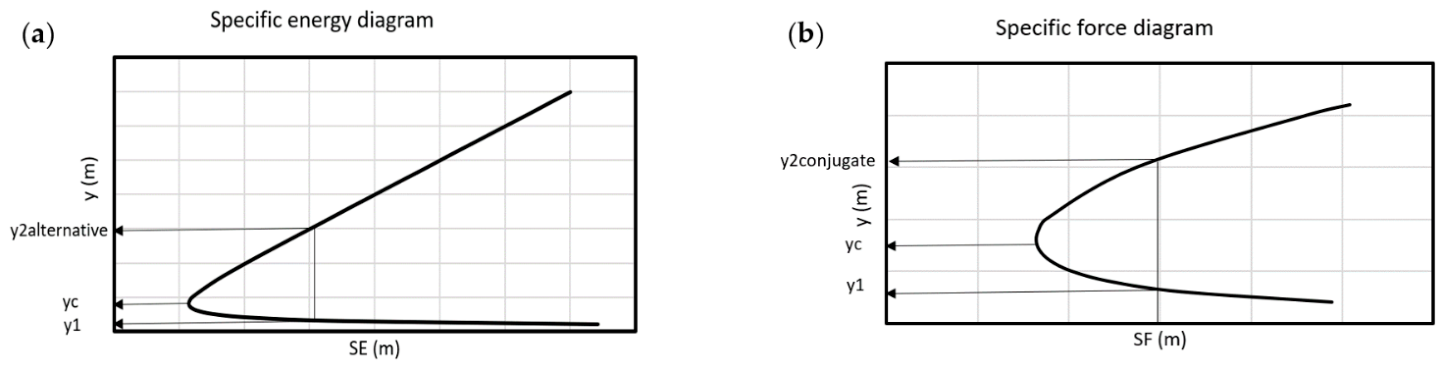
Local flow transitions were represented using two fundamental hydraulic principles: specific energy and specific force. These two principles are closely related in open-channel hydraulics, but they describe different physical mechanisms. Alternative depths are governed by equality of specific energy, whereas conjugate depths are governed by equality of specific force. To emphasize this conceptual parallel and improve the visual integration of the methodology, the specific-energy and specific-force diagrams were combined into one composite figure, as shown in Figure 3.

The alternative-depth problem was formulated using the specific-energy equation:

$$\mathrm{S}\mathrm{E}=\mathrm{y}+{\displaystyle \frac{{\mathrm{Q}}^2}{2\mathrm{g}{\mathrm{A}}^2}}$$

(9)

where (SE) is the specific energy. For a given discharge and channel geometry, two possible depths may correspond to the same value of specific energy, one supercritical and the other subcritical. Model 5 was trained to predict the alternative subcritical depth corresponding to a specified supercritical depth. The output variable was expressed as (${\displaystyle \frac{{\mathrm{y}}_{\left\{2,\mathrm{a}\mathrm{l}\mathrm{t}\right\}}}{{\mathrm{y}}_{\mathrm{c}}}}$), and the inputs were (Q), (b), (t), and (${\displaystyle \frac{{\mathrm{y}}_1}{{\mathrm{y}}_{\mathrm{c}}}}$), where (${\mathrm{y}}_1$) is the initial supercritical depth.

The conjugate-depth problem was formulated using the specific-force equation, which combines the hydrostatic and momentum components:

$$\mathrm{S}\mathrm{F}=\mathsf{\gamma }\mathrm{A}{\mathrm{h}}_{\mathrm{c}\mathrm{e}\mathrm{n}\mathrm{t}\mathrm{r}\mathrm{o}\mathrm{i}\mathrm{d}}+{\displaystyle \frac{{\mathsf{\gamma }\mathrm{Q}}^2}{\mathrm{g}\mathrm{A}}}$$

(10)

$$\mathrm{A}{\mathrm{h}}_{\mathrm{c}\mathrm{e}\mathrm{n}\mathrm{t}\mathrm{r}\mathrm{o}\mathrm{i}\mathrm{d}}={\displaystyle \frac{{\mathrm{b}\mathrm{y}}^2}{2}}+{\displaystyle \frac{\mathrm{t}{\mathrm{y}}^3}{3}}$$

(11)

where (SF) is the specific force, (γ) is the specific weight of water, and (${\mathrm{h}}_{\mathrm{c}}$) is the vertical distance between the water surface and the centroid of the wetted area. For a trapezoidal section, the first moment of area was evaluated consistently with the section geometry. Model 6 predicted the conjugate depth associated with a specified supercritical depth, expressed as (${\displaystyle \frac{{\mathrm{y}}_{\left\{2,\mathrm{c}\mathrm{o}\mathrm{n}\right\}}}{{\mathrm{y}}_{\mathrm{c}}}}$). The inputs were the same as those used for the alternative-depth model: (Q), (b), (t), and (${\displaystyle \frac{{\mathrm{y}}_1}{{\mathrm{y}}_{\mathrm{c}}}}$). This separation between Models 5 and 6 is important because alternative depths are governed by energy equivalence, whereas conjugate depths are governed by momentum conservation.

2.2.4. Gradually Varied Flow Formulation

The gradually varied flow (GVF) models were formulated to represent the longitudinal variation of water depth in prismatic open-channel reaches under steady nonuniform flow conditions. In GVF, the water depth changes gradually along the channel because of the imbalance between the bed slope and the friction slope. This type of flow is commonly encountered upstream of control structures, such as gates, weirs, and transitions, where the downstream boundary condition influences the upstream water-surface profile.

The governing equation for one-dimensional steady GVF can be written as

$${\displaystyle \frac{\mathrm{d}\mathrm{y}}{\mathrm{d}\mathrm{x}}}={\displaystyle \frac{{\mathrm{S}}_{\mathrm{o}}-{\mathrm{S}}_{\mathrm{f}}}{1-\frac{{\mathrm{Q}}^2\mathrm{B}}{\mathrm{g}{\mathrm{A}}^3}}}$$

(12)

where (y) is the flow depth, (x) is the longitudinal distance, (${\mathrm{S}}_{\mathrm{o}}$) is the bed slope, (${\mathrm{S}}_{\mathrm{f}}$) is the friction slope, (Q) is the discharge, (B) is the water-surface top width, (A) is the flow area, and (g) is gravitational acceleration. The denominator of this equation reflects the effect of the Froude number, while the numerator represents the difference between the channel-bed slope and the energy slope. Therefore, the equation links the spatial change in flow depth to both channel geometry and hydraulic resistance.

The friction slope (${\mathrm{S}}_{\mathrm{f}}$) was evaluated using Manning’s equation as

$${\mathrm{S}}_{\mathrm{f}}={\left.\left({\displaystyle \frac{\mathrm{Q}\mathrm{n}}{\mathrm{A}{\mathrm{R}}^{\left\{\frac{2}{3}\right\}}}}\right.\right)}^2$$

(13)

The GVF equation is nonlinear and normally requires numerical integration. This makes GVF analysis a suitable case for ANN surrogate modeling, particularly when many profile calculations are required in design iterations, optimization, sensitivity analysis, or inverse hydraulic estimation.

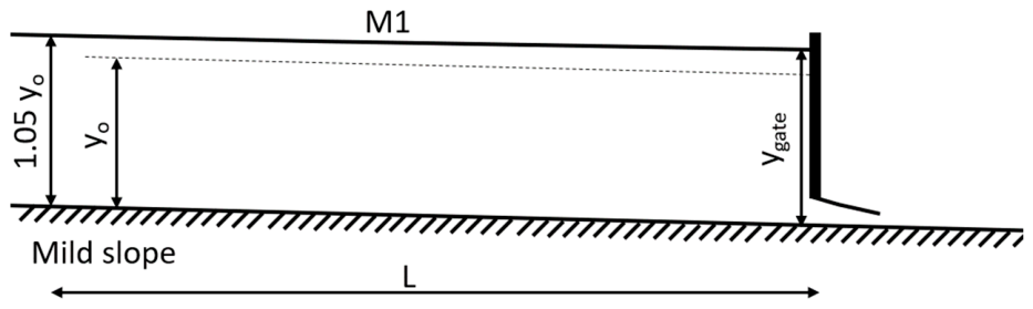
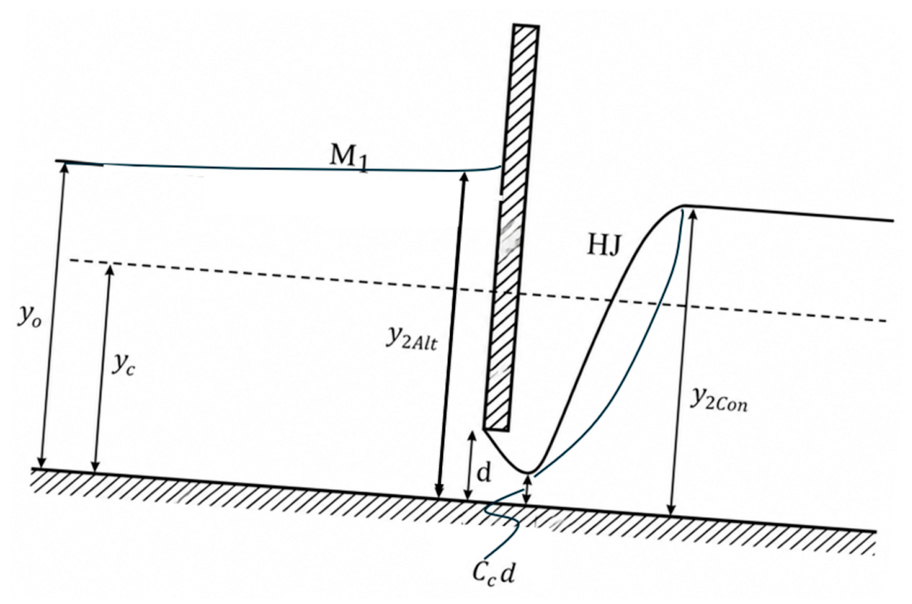
Model 7 was developed for a mild trapezoidal reach controlled by a downstream gate. The reach had a bed width from 2 to 10 m, a side slope from 1H:1V to 3H:1V, Manning’s coefficient from 0.01 to 0.035, and a bed slope of 0.00005. Under these hydraulic conditions, the downstream gate produces an M1 backwater curve upstream of the control section. Since an M1 profile approaches the normal-depth line asymptotically in the upstream direction, its theoretical length is very large. Therefore, for practical ANN formulation, the water-surface-profile length was defined from the section where the water depth is equal to (1.05y_o) to the section immediately upstream of the gate, where the depth is (y_gate). The hydraulic definition of this mild-slope case is illustrated in Figure 4.

For Model 7, the ANN input variables were the bed width, side slope, Manning’s coefficient, Froude number at normal depth, and the ratio between the water-surface-profile length (L) and bed width, while the output variable was the relative gate depth (${\displaystyle \frac{{\mathrm{y}}_{\left\{\mathrm{g}\mathrm{a}\mathrm{t}\mathrm{e}\right\}}}{{\mathrm{y}}_{\mathrm{o}}}}$). The reference values used for training were generated by numerically solving the GVF differential equation using MATLAB (v2024). This model therefore provides a direct surrogate relationship between discharge, profile length, and the downstream-controlled water depth in a mild-slope channel.

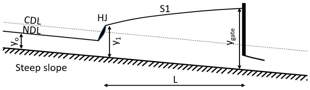
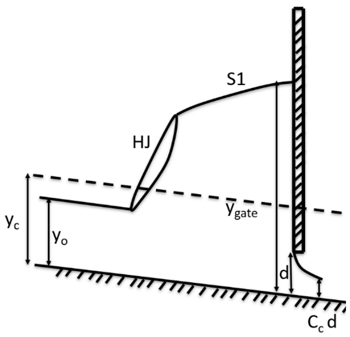
Model 8 was developed for a steep trapezoidal reach controlled by a downstream gate. The reach had the same ranges of bed width, side slope, and Manning’s coefficient as the mild-slope case, while the bed slope was increased to 0.01. Under these conditions, the normal depth is smaller than the critical depth and the approach flow is therefore supercritical. The downstream gate imposes a subcritical control, requiring a hydraulic jump between the supercritical approach flow and the downstream-controlled S1 backwater profile. The hydraulic jump itself was not calculated using the GVF equation. For each hydraulic realization, the normal depth and critical depth were first determined. The supercritical approach depth immediately upstream of the jump was represented by the normal depth, and the corresponding downstream conjugate depth was then calculated from equality of specific force, i.e., from the momentum relation described in Section 2.2.3. This conjugate depth defines the upstream boundary condition of the subcritical S1 profile. The GVF equation was subsequently integrated only over the gradually varied reach extending from the downstream side of the hydraulic jump to the section immediately upstream of the gate. Accordingly, the water-surface-profile length for Model 8 was defined between the hydraulic-jump location and the downstream gate-controlled section, as illustrated in Figure 5.

For Model 8, the ANN input variables were the bed width, side slope, Manning’s coefficient, Froude number evaluated at normal depth (y_o), and the normalized S1-profile length, while the output variable was the relative gate depth y_gate/y_o. The reference outputs were generated after first establishing the post-jump conjugate depth through the momentum-based specific-force relation and then numerically integrating the GVF equation over the downstream subcritical S1 reach. Thus, Model 8 does not use the GVF equation to represent the discontinuous hydraulic-jump transition; rather, the jump supplies the upstream boundary condition for the gradually varied portion of the profile. This formulation allows the ANN surrogate to reproduce the downstream-controlled S1 response while maintaining the physical distinction between rapidly varied flow at the hydraulic jump and gradually varied flow along the backwater reach

2.2.5. Water-Surface-Profile Mapping and Inverse Discharge Estimation

To support the inverse-discharge analysis presented later in the paper, Model 9 was formulated as a profile-mapping ANN. Unlike Models 7 and 8, which predict a depth ratio from discharge and profile length, Model 9 predicts the spatial distribution of water depths upstream of a control section. The input variables were the discharge (Q) and the downstream-control depth (${\mathrm{y}}_{\mathrm{g}\mathrm{a}\mathrm{t}\mathrm{e}}$). The output vector consisted of water depths at specified upstream distances of 500, 1000, 1500, 2000, 2500, 3000, 3500, 4000, 4500, and 5000 m.

The forward use of Model 9 provides rapid estimation of a water-surface profile for a known discharge and downstream water level. The inverse use was implemented by treating discharge as an unknown candidate variable. For each assumed discharge, Model 9 predicts the corresponding water-depth vector. The predicted vector is then compared with a reference or observed water-surface profile using the mean squared error. The discharge producing the minimum error is selected as the ANN-based estimate of the flow rate. This procedure provides a computationally efficient proof of concept for discharge estimation from water-level observations, provided that the geometry, roughness, slope, and downstream boundary condition remain within the domain used to train the model.

2.3. Synthetic Data Generation

The ANN datasets were generated synthetically by solving the governing hydraulic equations over predefined parameter ranges. This approach ensured that the training targets were hydraulically informed and directly linked to classical open-channel theory. Random combinations of the input variables were generated using uniform sampling over the selected ranges, and the corresponding output variables were obtained by solving the relevant implicit hydraulic equation or by numerically integrating the GVF equation.

For Models 1–4, 40,000 combinations were generated for each model. The trapezoidal normal-depth model covered (${\displaystyle \frac{{\mathrm{A}·\mathrm{R}}^{2/3}}{{\mathrm{b}}^{8/3}}}$) values from 5 × 10⁻⁴ to 8600 and side slopes of 0, 0.5, 1, 1.5, 2, 2.5, 3, 3.5, 4, 4.5, 5, and 10. The circular normal-depth model covered (${\displaystyle \frac{{\mathrm{A}·\mathrm{R}}^{2/3}}{{\mathrm{D}}^{8/3}}}$) values from 1.6384 × 10⁻¹⁰ to 0.335. The trapezoidal critical-depth model covered (${\displaystyle \frac{\mathrm{Q}}{\sqrt{\mathrm{g}}·{\mathrm{b}}^{5/2}}}$) values from 0.0011 to 6200 with the same set of side slopes. The circular critical-depth model covered (${\displaystyle \frac{\mathrm{Q}}{\sqrt{\mathrm{g}}·{\mathrm{D}}^{5/2}}}$)) values from 0.017638 to 16.

For Models 5 and 6, 65,000 combinations were generated for each model. The discharge varied from 0.005 to 100 m³/s, the bed width varied from 0.5 to 30 m, and the side slope followed the same values used for the trapezoidal normal- and critical-depth models. The gravitational acceleration has a range between 9.7639 m/s² to 9.8337 m/s². The supercritical input depth was represented by the ratio (${\displaystyle \frac{{\mathrm{y}}_1}{{\mathrm{y}}_{\mathrm{c}}}}$), with values from 0.05 to 0.9. The target values were obtained by solving the specific-energy equation for Model 5 and the specific-force equation for Model 6.

For the GVF-related models, the reference datasets were generated by numerical integration of the GVF differential equation using MATLAB (v2024). For the mild-slope case, approximately 100,000 combinations were produced over a wide range of discharge and profile length values. For the steep-slope case, the dataset-generation procedure additionally accounted for the hydraulic jump. For each realization, the normal and critical depths were first calculated, the post-jump conjugate depth was obtained from the specific-force relation, and this depth was then used as the upstream boundary condition for numerical integration of the downstream S1 profile using the GVF equation.

Table 1. Input parameters versus output parameter for all networks.

ANN Model	X-Section Shape		Governing Equation				Objective of Calculation							Model (I/O)
	Trapezoidal	Circular	Uniform Using Manning	Specific Energy	Specific Force	GVF ODE	Normal	Critical	Alt.	Conj.	Depth at Distance	Gate or Dam	WSP	Input Parameters	Output Target
1	✔		✔				✔							Log[AR2/3/b8/3], t	Log[yo/b]
2		✔	✔				✔							Log[AR2/3/d8/3]	Log[ϴo]
3	✔			✔				✔						Log[Q/(g0.5b2.5)], t	Log[yc/b]
4		✔		✔				✔						Log[Q/(g0.5d2.5)]	Log[ϴc]
5	✔			✔					✔					Q, b, t, g, y1/yc	Log[y2alt/yc]
6	✔				✔					✔				Q, b, t, g, y1/yc	Log[y2con/yc]
7	✔					✔					✔	✔	✔	b, t, n, Fn @ yo, L/b	ygate/yo
8	✔					✔					✔	✔	✔	b, t, n, Fn@ yo, L/b	ygate/yo
9	✔					✔					✔	✔	✔	Q, ygate	y at upstream distances = 500, 1000, 1500, 2000, 2500, 3000, 3500, 4000, 4500, and 5000 m
10	✔												✔	Q, W.L.1	W.L.5

Note: ✔ = parameter/condition applied.

summarizes the input variables, output variables, and governing hydraulic formulation associated with each ANN model. The descriptive statistics of the corresponding input and output variables are subsequently presented in

Table 2. Descriptive statistics for input and output parameters for all networks.

ANN Model	Input					Output	Parameter Notation	Mean	Median	Mode	Std. Dev.	Sample Variance	Kurtosis	Skewness	Range	Min	Max
	Input Parameter 1	Input Parameter 2	Input Parameter 3	Input Parameter 4	Input Parameter 5	Output Target
1	✔						A·R2/3/b8/3	728	232	2624	1171	1,371,783	12	3	8665	0+	8665
		✔					t	3.125	2.75	5	2.6	6.6	1.7	1.3	10	0+	10
						✔	y/b	7.5	7.5	5.1	4.3	18.7	−1.2	−0.0017	14.99	0.01	15
2	✔						A·R2/3/d8/3	0.132	0.093	0.014	0.125	0.016	−1.44	0.405	0.335	0+	0.335
						✔	ϴ (degree)	76°	76°	45°	43°	1892	−1	0	151°	0	151°
3	✔						Q/sqrt(g)/b2.5	12	5	9	16	261	9	3	115	0	115
		✔					t	3.1	2.8	5	2.6	6.6	1.7	1.3	10	0	10
						✔	y/b	1.5	1.51	0.43	0.86	0.74	−1.2	0	2.99	0.01	3
4	✔						Q/sqrt(g)/d2.5	0.52	0.25	0.03	0.88	0.78	65.7	6.16	16.22	0	16.22
						✔	ϴ (degree)	90	90	46	52	2709	−1	0	180	0	180
5	✔						Q	49.5	49	1.9	28.9	837	−1.2	0	100	0	100
		✔					b	15.2	15.2	17.6	8.5	72.3	−1.2	0	29.5	0.5	30
			✔				t	3.1	3	5	2.6	6.5	1.7	1.3	10	0	10
				✔			g	9.80	9.80	9.79	0.02	0.00	−1.20	0.00	0.07	9.76	9.83
					✔		y1/yc	0.45	0.45	0.05	0.28	0.08	−1.28	0.07	0.85	0.05	0.90
						✔	y2alt/yc	58	4		305	93,263	489	19	10,328	1	10,329
6	✔						Q	49.53	48.99	89.41	28.93	837.01	−1.2	0.03	100	0	100
		✔					b	15.23	15.17	17.62	8.5	72.31	−1.2	0	29.5	0.5	30
			✔				t	3.13	3	5	2.56	6.54	1.66	1.33	10	0	10
				✔			g	9.80	9.80	9.79	0.02	0.00	−1.20	0.00	0.07	9.76	9.83
					✔		y1/yc	0.45	0.45	0.05	0.28	0.08	−1.28	0.07	0.85	0.05	0.90
						✔	y2conj/yc	2.37	1.86	1.11	1.34	1.79	0.59	1.27	5.82	1.11	6.93
7	✔						b	6.00	6.01	6.64	2.30	5.28	−1.19	0.00	8.00	2.00	10.00
		✔					t	2.00	2.00	2.50	0.61	0.38	−1.00	0.00	2.00	1.00	3.00
			✔				n	0.022	0.022	0.033	0.007	0.000	−1.20	0.009	0.025	0.01	0.035
				✔			Fn @ yo	0.102	0.104	0.106	0.006	0.000	3.61	−1.658	0.055	0.05	0.108
					✔		L/b	6230	6250	0	3951	15,612,020	−1	0	12,500	0	12,500
						✔	ygate/yo	1.43	1.27	1.05	0.56	0.32	24.7	4.21	5.94	1.05	6.99
8	✔						b	6.00	6.01	6.64	2.30	5.28	−1.19	0.00	8.00	2.00	10.00
		✔					t	2.00	2.00	2.50	0.61	0.38	−1.00	0.00	2.00	1.00	3.00
			✔				n	0.022	0.022	0.033	0.007	0.000	−1.20	0.009	0.025	0.01	0.035
				✔			Fn @ yo	1.244	1.260	1.294	0.052	0.003	1.89	−1.446	0.264	1.04	1.299
					✔		L/b	42.8	37.5	0.0	31.4	985.9	−0.9	0.4	112.5	0.0	112.5
						✔	ygate/yo	3.99	4.00	1.32	1.76	3.09	−1.18	−0.04	5.95	1.05	7.00
9	✔						Q	521.4	520.1	743.6	272.1	74,043.6	−1.2	0.0	949.9	50.1	1000.0
		✔					ygate	4.14	4.36	5.06	1.14	1.29	−0.38	−0.62	5.12	0.88	6.00
						✔	y	3.86	4.05	5.06	1.12	1.27	−0.56	−0.54	5.12	0.88	6.00
10	✔						Q	7354	8000	12,000	3577	12,793,324	−1.35	−0.13	10,205	2000	12,000
		✔					WL1	231	231	229	1.05	1.09	−1.49	0.16	2.70	229	232
						✔	WL5	232	232	232	1.03	1.06	−0.69	−0.39	4	229	234

Notes: The notation (0+) denotes a value greater than zero but smaller than the reporting precision adopted in the table; therefore, it is shown as nearly zero after rounding. The descriptive statistics reported for Model 10 refer only to the HEC-RAS-generated dataset used for ANN development. The independently measured field case used for inverse-discharge evaluation is not included in these statistics. ✔ = parameter/condition applied.

.

2.4. ANN Architecture, Preprocessing, and Training

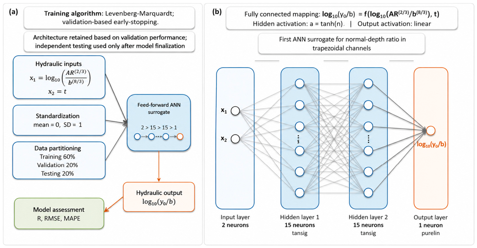
A feed-forward ANN structure was adopted because the objective was to approximate deterministic nonlinear mappings between hydraulic input variables and target hydraulic quantities. The detailed architecture shown in Figure 6 illustrates the structure used for Model 1. The input layer contains two neurons corresponding to (${\displaystyle \frac{{\mathrm{A}·\mathrm{R}}^{2/3}}{{\mathrm{b}}^{8/3}}}$) and (t), followed by two hidden layers. Each hidden layer contains fifteen neurons with a hyperbolic tangent sigmoid transfer function. The output layer contains one neuron with a linear transfer function, corresponding to (${\displaystyle \frac{{\mathrm{y}}_{\mathrm{o}}}{\mathrm{b}}}$).

The same methodological training philosophy was applied to the remaining ANN models, with the number of input and output neurons adjusted according to the input–output definitions listed in Table 1. The hidden layer structure was selected through trial training, considering both prediction accuracy and generalization capability. The final architecture was retained when the training and validation results showed a high correlation between ANN outputs and reference targets without evidence of overfitting. To provide a quantitative assessment of the retained architecture, an additional architecture sensitivity analysis was conducted for Model 1 using alternative one- and two-hidden-layer configurations and repeated training with different weight initializations. The analysis showed that the retained architecture provided the most favorable overall balance among validation accuracy, run-to-run stability, convergence behavior, and model complexity. The complete architecture sensitivity methodology and results are provided in Supplementary Section S2, including Table S1 and Figures S3 and S4.

Before training, all input and output variables were standardized to have zero mean and unit standard deviation. This preprocessing step reduces scale imbalance among variables and improves the numerical conditioning of the ANN optimization process. Each dataset was divided into three mutually exclusive subsets: 60% for training, 20% for validation, and 20% for independent testing. The training subset was used to update the network weights and biases, the validation subset was used to monitor generalization and apply early stopping, and the testing subset was reserved for independent performance assessment after training.

The Levenberg–Marquardt algorithm was used for network training because of its efficiency for supervised feed-forward neural networks with moderate dimensionality. The mean squared error was used as the performance function during training. The principal training settings adopted for Model 1 are summarized in

Table 3. Typical example for training algorithm and control parameters adopted for ANN Model 1.

Training:	Levenberg–Marquardt
Performance:	Mean Squared Error
Calculations:	MEX
Performance target value:	0
Gradient target value:	1.00 × 10−7

.

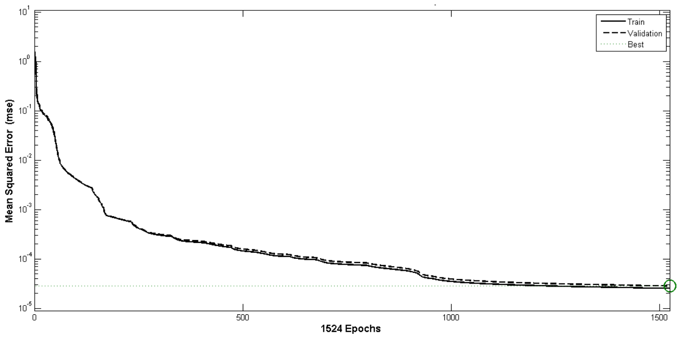
For Model 1, the convergence history is shown in Figure 7. The validation error reached its minimum at epoch 1524, and training was terminated at this point using validation-based early stopping. This procedure retained the network weights associated with the best out-of-sample performance and reduced the risk of overfitting.

2.5. Model Evaluation

The trained ANN models were evaluated using independent testing datasets that were not involved in the training or validation stages. This independent assessment was necessary to examine whether the developed networks were able to generalize the hydraulic relationships learned from the synthetic datasets rather than merely reproduce the training samples. Model performance was quantified using the correlation coefficient (R), root mean squared error (RMSE), and mean absolute percentage error (MAPE). The correlation coefficient was used to assess the strength of agreement between the predicted and reference values, while RMSE and MAPE were used to quantify the absolute and relative magnitudes of prediction error, respectively.

In addition to these indicators, the mean absolute error (MAE) and Kling–Gupta efficiency (KGE) were used to provide complementary measures of model performance. MAE quantifies the average magnitude of the prediction error in the original output scale and is less sensitive to isolated large deviations than RMSE. KGE provides an integrated assessment of agreement by simultaneously accounting for correlation, relative variability, and bias between ANN predictions and reference values. A KGE value approaching unity therefore indicates strong overall agreement. 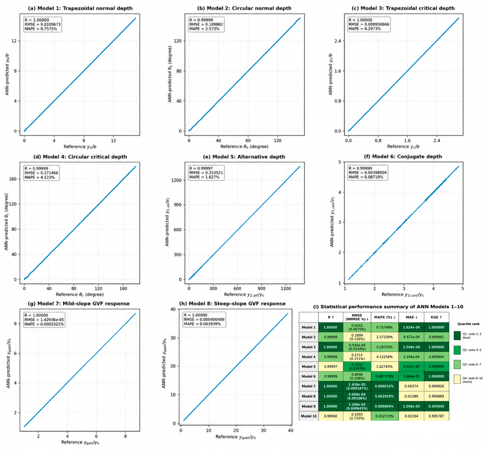These additional indicators were particularly useful for the extended statistical comparison presented in Figure 8i, which includes the performance of all ten ANN models.

The evaluation was carried out at two complementary levels. First, the direct predictive accuracy of the ANN models was assessed by comparing the network outputs with the hydraulic reference values generated from the governing equations and numerical procedures described in the previous subsections. This assessment was applied to the normal-depth, critical-depth, alternative-depth, conjugate-depth, and GVF-related ANN models. Second, the hydraulic usefulness of the proposed framework was examined through application-oriented comparisons, including water-surface-profile prediction and inverse discharge estimation from spatial water-depth information.

This evaluation strategy provides the basis for the results presented in the following section. Section 3 first examines the agreement between ANN predictions and reference hydraulic solutions for the individual models. It then evaluates the ability of the GVF models to reproduce mild- and steep-slope water-surface profiles. Finally, it demonstrates the inverse-discharge application, in which the trained ANN framework is used to infer discharge from a known or observed longitudinal water-depth profile. The statistical indicators reported in this subsection will be interpreted together with the hydraulic comparisons presented in Section 3.

2.6. Scope and Assumptions

The proposed ANN models are valid within the hydraulic ranges used to generate the training datasets. Because the datasets were generated from classical hydraulic equations and numerical procedures, the trained networks reproduce the behavior of these formulations rather than field measurements affected by irregular geometry, spatially variable roughness, vegetation, sediment transport, unsteady flow, turbulence, or measurement uncertainty. Therefore, the models should be interpreted as fast hydraulic surrogates for well-defined open-channel flow calculations, not as universal predictors for all field conditions.

The GVF and inverse-discharge models are particularly dependent on the assumed reach geometry, Manning’s coefficient, bed slope, and downstream boundary condition. Application to other channel configurations requires retraining or extending the input space to include geometry, roughness, slope, and boundary variables. With these assumptions clearly defined, the methodology provides the basis for the results and discussion in Section 3, where the trained ANN models are evaluated for normal-depth, critical-depth, local-transition, GVF, and inverse-discharge applications.

3. Results and Discussion

The results of this study demonstrate that artificial neural networks (ANNs) can provide accurate and computationally efficient surrogate models for several nonlinear open-channel hydraulics problems that are traditionally solved using iterative numerical procedures. The high level of agreement between the ANN outputs and the reference hydraulic solutions indicates that the trained networks successfully reproduced the dominant relationships governing uniform flow, critical flow, local hydraulic transitions, gradually varied flow (GVF), and profile-based discharge estimation. However, the significance of these results is not limited to statistical agreement. From a hydraulic perspective, the results indicate that the proposed framework approximated the functional behavior of several governing formulations, including Manning’s equation, the critical-flow condition, the specific-energy equation, the specific-force equation, and the GVF differential equation.

The proposed framework is therefore not simply a black-box correlation between input and output data. The ANN inputs were selected to reflect physically meaningful hydraulic variables and, where appropriate, dimensionless or normalized parameters. This is important because open-channel flow behavior is controlled by scaling relationships among discharge, gravity, channel geometry, flow resistance, bed slope, hydraulic radius, and flow depth. By training the networks using variables that preserve these hydraulic dependencies, the models reproduced the response of the governing equations within the investigated hydraulic ranges. This supports the use of ANN models as fast hydraulic surrogates, particularly when repeated calculations are required in design iterations, optimization routines, sensitivity analysis, or inverse hydraulic assessment.

3.1. Prediction Performance of ANN Models

The predictive performance of the developed ANN models is summarized in Figure 8. Panels 8a–h provide direct comparisons between ANN-predicted values and the corresponding MATLAB (v2024) reference solutions for Models 1–8, whereas Figure 8i extends the statistical assessment to all ten ANN models, including Models 9 and 10. In panels 8a–h, the 1:1 line represents perfect agreement between the ANN predictions and the corresponding reference hydraulic solutions. Accordingly, the proximity of the plotted points to this line provides a direct visual indication of predictive accuracy. Panel 8i complements these scatter comparisons using the correlation coefficient (R), root mean squared error (RMSE), range-normalized RMSE (NRMSE), mean absolute percentage error (MAPE), mean absolute error (MAE), and Kling–Gupta efficiency (KGE). To facilitate compact comparison among models having different output variables and numerical scales, the cell shading is based on the relative rank of each model within each performance metric, as described below, while the numerical values displayed in the cells remain the primary quantitative performance information.

The general agreement pattern in Figure 8a–h shows that the ANN predictions are closely clustered around the 1:1 equality line for all eight hydraulic mappings. This confirms that the trained networks did not merely capture broad trends but also reproduced the magnitudes of the reference MATLAB solutions over the evaluated ranges. The absence of a visually systematic departure from the equality line indicates that no clear global overprediction or underprediction bias was introduced by the ANN models. This behavior is particularly important because the eight networks represent different hydraulic mechanisms, as mentioned earlier.

For the normal-depth models, Figure 8a,b show that the ANN framework accurately reproduced the nonlinear relationships embedded in Manning’s equation. Model 1, which predicts the relative normal depth (${\displaystyle \frac{{\mathrm{y}}_{\mathrm{o}}}{\mathrm{b}}}$) for trapezoidal sections, achieved (R = 1.00000), RMSE = 0.010067, and MAPE = 0.757485%. This strong performance indicates that the model captured the combined effects of flow area, wetted perimeter, hydraulic radius, and side slope on channel conveyance. In trapezoidal sections, these geometric quantities vary nonlinearly with water depth, especially when the side slope is large or when the depth becomes comparable to the bed width. The close agreement in Figure 8a therefore confirms that the ANN model successfully replaced the implicit Manning equation solution with a direct hydraulic mapping.

Model 2, which predicts the normal-depth angle (${\mathsf{\theta }}_{\mathrm{o}}$) for circular sections, also performed strongly, with (R = 0.99999), RMSE = 0.189882°, and MAPE = 2.573390%. The slightly larger relative error compared with Model 1 is hydraulically reasonable because circular-section flow is controlled by angular geometry. In partially full circular sections, the wetted area, wetted perimeter, hydraulic radius, and water depth are all nonlinear functions of the central angle. Small angular deviations may therefore become more influential under shallow or nearly full conditions. Nevertheless, the performance of Model 2 remains highly accurate and confirms that the adopted logarithmic transformation improved the representation of circular-section conveyance over a wide range of filling conditions.

The critical-depth models are evaluated in Figure 8c,d. Model 3, which predicts the relative critical depth (${\displaystyle \frac{{\mathrm{y}}_{\mathrm{c}}}{\mathrm{b}}}$) in trapezoidal channels, produced (R = 1.00000), RMSE = 0.000951, and MAPE = 0.297326%. This result indicates that the ANN captured the critical-flow condition associated with minimum specific energy and a Froude number equal to unity. Unlike normal depth, critical depth is independent of Manning’s roughness coefficient and bed slope; it is governed by the balance between inertial and gravitational effects. The high accuracy of Model 3 therefore demonstrates that the ANN framework can reproduce inertia–gravity hydraulic transitions, not only resistance-based flow relationships.

Model 4 extended the critical-depth prediction to circular sections and achieved (R = 0.99999), RMSE = 0.271466°, and MAPE = 4.122576%. Although this is the largest MAPE among the eight ANN models, the corresponding correlation coefficient remains almost unity and the RMSE remains small in angular terms. The relatively higher MAPE reflects the stronger geometric nonlinearity of circular critical flow rather than weak predictive capability. In circular sections, both the flow area and the top width vary nonlinearly with the central angle, and the critical-flow equation becomes sensitive when the flow occupies a small or large portion of the pipe. Consequently, a small angular prediction difference may generate a relatively larger percentage error. This makes Model 4 one of the most demanding hydraulic mappings in the proposed framework.

The local-transition models are shown in Figure 8e,f. Model 5 predicts the alternative-depth ratio (${\displaystyle \frac{{\mathrm{y}}_{2,\mathrm{a}\mathrm{l}\mathrm{t}}}{{\mathrm{y}}_{\mathrm{c}}}}$), which is governed by equality of specific energy. It achieved (R = 0.99997), RMSE = 0.333521, and MAPE = 1.627434%. The RMSE of Model 5 is the largest among the eight models, but this should be interpreted in relation to the broad numerical range of the alternative-depth ratio. Alternative depths can vary substantially when the supercritical input depth is far below the critical depth, producing large subcritical alternative depths for the same specific energy. Therefore, the larger raw RMSE mainly reflects the scale and spread of the target variable rather than a failure of the ANN model. The moderate MAPE confirms that the relative prediction error remained acceptable despite the wide output range.

Model 6 predicts the conjugate-depth ratio (${\displaystyle \frac{{\mathrm{y}}_{2,\mathrm{c}\mathrm{o}\mathrm{n}}}{{\mathrm{y}}_{\mathrm{c}}}}$), which is governed by equality of specific force and momentum conservation across a hydraulic jump. This model produced (R = 0.99999), RMSE = 0.003980, and MAPE = 0.087178%, indicating very strong agreement with the reference solution. The lower error level compared with Model 5 is physically meaningful because the conjugate-depth ratio has a narrower numerical range than the alternative-depth ratio. The performance of Models 5 and 6 confirms that the ANN framework can reproduce two distinct conservation-law-based hydraulic transitions: energy equivalence for alternative depths and momentum equivalence for conjugate depths. This is important for hydraulic applications involving gates, contractions, hydraulic jumps, and energy-dissipation structures.

The GVF-related models, shown in Figure 8g,h, produced the smallest errors among all models. Model 7, developed for the mild-slope gate-controlled reach, achieved (R = 1.00000), RMSE = (1.4 × 10⁻⁵), and MAPE = 0.000532%. Model 8, developed for the steep-slope gate-controlled reach, achieved (R = 1.00000), RMSE = 0.000400, and MAPE = 0.003939%. These very small errors indicate that the ANN models reproduced the relationship among discharge, water-surface-profile length, and relative gate depth with very high precision for the investigated channel configurations. This result is significant because GVF profiles are governed by a nonlinear differential equation whose solution normally requires stepwise numerical integration. The ANN models therefore provide efficient surrogates for repeated GVF calculations within the hydraulic ranges used for training.

The statistical summary in Figure 8i provides a relative performance comparison of all ten ANN models using rank-quartile shading. For each metric, the ten models were ranked independently according to the preferred direction of performance: higher values are preferred for and KGE, whereas lower values are preferred for NRMSE, MAPE, and MAE. The resulting ranks were grouped into four classes: Q1 comprises ranks 1–3 and represents the strongest relative performance; Q2 comprises ranks 4–5; Q3 comprises ranks 6–7; and Q4 comprises ranks 8–10 and represents the comparatively lowest performance within that metric. For RMSE, the ranking was based on the corresponding range-normalized value (NRMSE) to reduce the influence of differences in output magnitude and units, while the original RMSE value is retained in each cell for direct reference. Thus, the color scale represents relative rank within each metric rather than an absolute error threshold.

This ranking should therefore be interpreted together with the numerical values rather than independently. In particular, assignment to a lower rank quartile does not necessarily indicate poor predictive performance, because several metrics are tightly clustered near their theoretical optimum. For example, the MAE and KGE values of most models remain very close to unity even when their relative ranks differ. Conversely, the NRMSE and MAPE columns provide greater discrimination among models because they express prediction errors relative to the scale of the corresponding outputs. Overall, Figure 8i confirms strong predictive performance across the ten ANN models while providing a compact means of identifying their relative strengths under different statistical criteria.

For RMSE, the shading is based on range-normalized RMSE rather than raw RMSE. This choice is important because the eight ANN models predict different hydraulic quantities with different units and numerical ranges, including depth ratios and angular variables expressed in degrees. A direct visual comparison of raw RMSE values across these outputs may be misleading because a larger RMSE can simply reflect a wider output range or a different physical scale. Normalizing RMSE by the corresponding output range provides a more balanced indication of the absolute error relative to the hydraulic scale of each model. The MAPE column is shaded using percentage error, which already represents a relative error measure.

Accordingly, Figure 8i should be interpreted as a compact error-intensity summary rather than as a simple ranking of the models. Lower color intensity indicates lower error, while darker cells identify cases where the error is relatively more noticeable within the adopted metric. The heat subplot shows that all eight ANN models achieved very strong agreement with the reference hydraulic solutions. The (R) values are nearly perfect for all models, confirming that the dominant monotonic relationships were preserved. The error metrics provide more detailed discrimination: Model 4 shows the largest relative error in terms of MAPE, which is consistent with the strong angular nonlinearity of critical flow in partially full circular sections, while Model 5 shows the largest raw RMSE because the alternative-depth ratio spans a much wider numerical range than most other outputs. Conversely, Models 7 and 8 show very low error intensity, reflecting the high accuracy of the GVF-related surrogate mappings for the investigated mild- and steep-slope channel configurations.

To examine whether the suitability of ANN was specific to a single hydraulic mapping, a comparative benchmark was conducted using four representative surrogate-learning methods: artificial neural networks (ANN), Random Forest (RF), support vector regression with a radial-basis-function kernel (SVR-RBF), and Gaussian Process Regression (GPR). The comparison was performed for three hydraulically distinct problems—Model 1, representing the smooth implicit normal-depth relationship; Model 5, representing the strongly nonlinear specific-energy alternative-depth problem; and Model 7, representing a GVF mapping originating from numerical integration of the governing differential equation. The competing methods were evaluated using common input–output data and consistent development and testing conditions, with model selection based on development data and final performance assessed on held-out test cases. The results demonstrate that no single learning method was universally superior across all hydraulic mappings and error measures. For Model 1, both ANN and GPR reproduced the smooth hydraulic relationship with extremely high accuracy, with GPR producing a slightly smaller absolute RMSE while ANN retained similarly negligible relative error. For Model 5, ANN provided the strongest overall predictive performance, yielding a MAPE of 0.775% compared with 3.155% for GPR, with RF and SVR producing larger errors. For Model 7, GPR achieved a modest advantage in absolute error (, RMSE = 0.4633) compared with ANN (, RMSE = 0.5136), whereas ANN showed substantially greater relative-error robustness, with a MAPE of 1.058% compared with 2.480% for GPR. Considered together with its compact fixed-size representation and low post-training inference cost, these results support ANN as a favorable accuracy–complexity–inference-efficiency compromise for the repeated hydraulic evaluations targeted in the present framework, rather than implying universal superiority over alternative machine-learning methods. Detailed model configurations, performance statistics, prediction comparisons, and accuracy–inference-cost results are provided in Supplementary Section S4.

3.2. Computational Efficiency Assessment

In addition to predictive accuracy, the computational efficiency of the ANN surrogates was assessed at two complementary levels. First, post-training inference time was compared directly with the runtime of the corresponding conventional iterative or numerical hydraulic procedure for Models 5–8, representing alternative-depth calculation, conjugate-depth calculation, and the mild- and steep-slope GVF applications, respectively. For each model, 10,000 identical input cases were evaluated using both approaches on the same computer. All computations were performed on a Dell Latitude 5400 laptop equipped with an eighth-generation Intel Core i5 processor, 8 GB of RAM, and a Windows 10 operating system. Second, because the ANN approach requires an initial offline investment for reference-dataset generation and network training, these development costs were incorporated into a break-even analysis to determine the number of repeated hydraulic evaluations required before the cumulative computational cost of the ANN approach becomes lower than that of repeated conventional calculations.

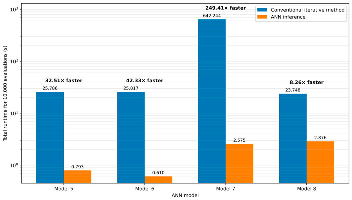
The runtime results are presented in Figure 9. For Model 5, the conventional iterative procedure required 25.786 s, whereas the ANN required 0.793 s, corresponding to a speedup of 32.5-fold. For Model 6, the respective runtimes were 25.817 and 0.610 s, producing a speedup of 42.3-fold. The largest computational gain was obtained for Model 7: conventional GVF calculations required 642.244 s, compared with only 2.575 s for ANN inference, corresponding to a speedup of 249.4-fold. For Model 8, the iterative and ANN runtimes were 23.748 and 2.876 s, respectively, giving a speedup of 8.26-fold.

Expressed on a per-evaluation basis, ANN inference required approximately 0.0793, 0.0610, 0.2575, and 0.2876 ms for Models 5–8, respectively, compared with 2.5786, 2.5817, 64.2244, and 2.3748 ms for the corresponding iterative calculations. Thus, all four evaluated models produced measurable computational acceleration, although the magnitude of the speedup varied according to the numerical workload of the corresponding conventional hydraulic solution. The particularly large acceleration for Model 7 reflects the computational burden associated with repeated numerical integration of the GVF equation over the mild-slope backwater profile. Overall, the results demonstrate that the computational advantage of the proposed framework is not restricted to one hydraulic equation but extends across energy-based, momentum-based, and spatial GVF calculations. These gains are especially relevant to optimization, sensitivity analysis, inverse estimation, and other applications requiring large numbers of repeated hydraulic evaluations.

Post-training inference speed alone does not provide a complete measure of computational efficiency because development of an ANN surrogate requires an initial offline investment. This investment includes generation of the hydraulic reference dataset, T_data, and ANN training, T_train. The total setup cost is therefore

T_setup = T_data + T_train.

For subsequent hydraulic evaluations, the cumulative conventional computational cost can be expressed as N_tconv, whereas the corresponding ANN cost is T_setup + N_tANN, where and are the per-evaluation conventional and ANN inference times, respectively. Equating these two costs gives the break-even number of evaluations,

$${\mathrm{N}}^{\mathrm{*}}={\displaystyle \frac{{\mathrm{T}}_{\mathrm{s}\mathrm{e}\mathrm{t}\mathrm{u}\mathrm{p}}}{{\mathrm{t}}_{\mathrm{c}\mathrm{o}\mathrm{n}\mathrm{v}}-{\mathrm{t}}_{\mathrm{A}\mathrm{N}\mathrm{N}}}}$$

Thus, N* represents the approximate number of repeated calculations required to recover the one-time computational investment associated with development of the ANN surrogate. Below this threshold, direct conventional calculation may remain computationally preferable; above it, the cumulative computational cost increasingly favors the trained surrogate.

The results in

Table 4. Model-development costs, per-evaluation computational times, and break-even thresholds for ANN Models 5–8.

ANN Model	Training Dataset Size (Ndata)	Dataset Gen. Time Tdata (s)	Network Training Time Ttrain (s)	Total Setup Time Tsetup (s)	Conv. Iterative Time Titer (ms/eval)	ANN Inference Time tANN (ms/eval)	Break-Even Threshold N* (Evaluations)
Model 5 (Alternative Depth)	10,000	25.786	45	70.786	2.5786	0.0793	28,322
Model 6 (Conjugate Depth)	65,000	167.8	40	207.8	2.5817	0.061	82,437
Model 7 (Mild-Slope GVF)	100,000	6422.40	180	6602.40	64.2244	0.2575	103,216
Model 8 (Steep-Slope GVF)	100,000	237.5	120	357.5	2.3748	0.2876	171,282

show that the break-even threshold depends strongly on both the computational burden of the original hydraulic calculation and the offline cost required to construct the surrogate. The corrected Model 5 calculation reaches break-even after approximately 2.83 × 10⁴ evaluations, whereas the thresholds for Models 6–8 are approximately, 8.24 × 10⁴, 1.03 × 10⁵, and 1.71 × 10⁵, and evaluations, respectively. Model 7 provides the largest post-training acceleration because each conventional evaluation requires numerical integration of the GVF equation. Although its dataset-generation cost is consequently the largest, the approximately 249-fold inference acceleration compensates for this initial investment after approximately 1.03 × 10⁵ evaluations. Beyond the break-even point, the computational advantage increases approximately linearly with the number of subsequent evaluations.

These results clarify that ANN surrogates are not necessarily advantageous for isolated one-off hydraulic calculations. Their principal computational benefit arises in high-throughput applications requiring repeated evaluation of the same hydraulic mapping, including sensitivity analysis, uncertainty propagation, Monte Carlo simulation, optimization, inverse estimation, and repeated operational assessment. The break-even analysis therefore complements the post-training comparison in Figure 9 by accounting explicitly for the one-time computational cost of surrogate development.

3.3. Numerical Cross-Verification of GVF-Related ANN Models Using HEC-RAS

The GVF-related ANN models were further evaluated through comparison with HEC-RAS simulations. This validation step is important because the scatter comparisons and statistical indicators presented earlier assess the ANN predictions against the generated reference datasets, whereas HEC-RAS provides an independent hydraulic benchmark for the spatial development of water-surface profiles. Accordingly, this comparison examines whether the ANN models reproduce not only point-based hydraulic variables, but also the longitudinal behavior of gradually varied flow profiles under downstream control.

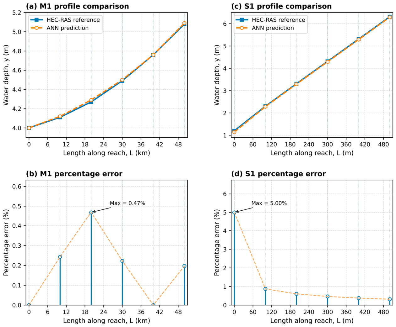
The validation results for the mild-slope and steep-slope cases are summarized in Figure 10. The figure combines the profile comparisons and percentage-error distributions for both hydraulic configurations. Figure 10a,b correspond to the mild-slope M1 profile, whereas Figure 10c,d correspond to the steep-slope S1 profile.

In the profile plots, the dashed ANN curves with markers identify the discrete comparison locations, while the solid curves represent the HEC-RAS reference results.

The mild-slope application, represented by the M1 profile, provides an important test of the framework because an M1 backwater curve approaches normal depth asymptotically in the upstream direction. Therefore, the theoretical profile length may become very large as the water depth approaches the normal-depth condition. In the present study, the profile length was defined using a practical upstream termination criterion based on a depth close to normal depth (+5%), which converted the theoretically long profile into a finite engineering quantity suitable for ANN training. Under these conditions, the seventh ANN learned the relationship among discharge, profile length, and gate-controlled depth for the fixed mild trapezoidal reach.

Figure 10a shows that the ANN-predicted M1 profile is in very close agreement with the HEC-RAS profile over the full 50 km reach. The near overlap between the two curves indicates that the ANN did not merely estimate the downstream-controlled depth, but also reproduced the longitudinal development of the backwater curve. The hydraulic trend is fully consistent with the expected behavior of an M1 profile: water depth increases toward the downstream gate because of the imposed downstream control, while the upstream part of the water surface gradually approaches the normal-depth condition. The ANN profile preserves this smooth and physically meaningful transition, indicating that the network captured the attenuation of the backwater influence along the channel.

The percentage-error distribution in Figure 10b confirms the high accuracy of the ANN prediction for the mild-slope case. The maximum percentage error is approximately 0.47%, occurring near the 20 km station, whereas the error is essentially zero at the downstream section and at the 40 km station. The remaining stations exhibit errors of only about 0.20–0.24%. These very small deviations show that the seventh ANN reproduced the HEC-RAS M1 profile with high fidelity over the entire reach. From a hydraulic perspective, this level of agreement is significant because the shape of an M1 backwater profile governs the upstream extent of downstream-control influence and is directly relevant to freeboard estimation, flood-level assessment, gate operation, and backwater evaluation upstream of hydraulic structures.

The steep-slope application, represented by the S1 profile, provides a more challenging hydraulic test because normal flow in a steep channel is supercritical, whereas the downstream gate imposes a subcritical depth upstream of the control section. This transition creates a hydraulically more complex condition involving a hydraulic jump upstream of the subcritical backwater region. Consequently, the eighth ANN was required to reproduce the combined influence of supercritical approach flow, hydraulic-jump-related momentum adjustment, and downstream gate control.

As shown in Figure 10c, the ANN-predicted S1 profile also agrees closely with the HEC-RAS results. The two profiles follow the same longitudinal trend, with water depth increasing downstream toward the gate-controlled section. This agreement indicates that the ANN successfully reproduced the spatial response of the steep-slope backwater system despite the more complex hydraulic setting. The ability of the ANN model to represent this profile is particularly important because steep-slope channels are highly sensitive to boundary control, and accurate prediction of the subcritical backwater region is essential for hydraulic design and safety assessment.

The percentage-error distribution in Figure 10d provides additional insight into the ANN performance for the S1 profile. The maximum percentage error occurs at the upstream end and is about 5.0%, after which the error decreases rapidly downstream to values below 1%. This trend is hydraulically reasonable because the upstream water depth is relatively small, and even a small absolute difference can produce a comparatively larger percentage error under shallow-flow conditions. As the flow depth increases downstream, the percentage error decreases, indicating stronger agreement between the ANN and HEC-RAS solutions within the deeper, gate-influenced part of the profile. Accordingly, the higher relative error near the upstream end should not be interpreted as a substantial model deficiency, but rather as a consequence of evaluating relative error at shallow depth. In practical terms, the absolute deviations remain small, and the overall agreement of the profile shape remains very good.

Taken together, the four panels in Figure 10 confirm that the ANN framework reproduced both mild-slope and steep-slope GVF profiles with strong agreement to HEC-RAS. The validation is important because it demonstrates that the ANN models preserved the spatial hydraulic behavior of the water-surface profiles, not only isolated predicted quantities. For the mild-slope reach, the seventh ANN accurately reproduced the gradual backwater rise toward the downstream gate. For the steep-slope reach, the eighth ANN successfully captured the downstream-controlled S1 profile despite the more complex hydraulic conditions associated with steep-bed flow. These findings support the use of the ANN models as rapid surrogates for GVF profile estimation within the hydraulic domains used for model development.

3.4. Profile-Based Inverse Discharge Estimation Using ANN Model

The ninth ANN model was developed to extend the proposed framework from direct hydraulic prediction to profile-based inverse discharge estimation. This application is more challenging than the preceding forward-prediction tasks because the discharge is not specified directly. Instead, the discharge is inferred from the degree of agreement between the ANN-predicted water-surface profile and a reference profile. From a practical hydraulic perspective, this type of inverse analysis is valuable when direct discharge measurements are unavailable or uncertain, whereas water-level observations along the channel reach can be obtained more readily.

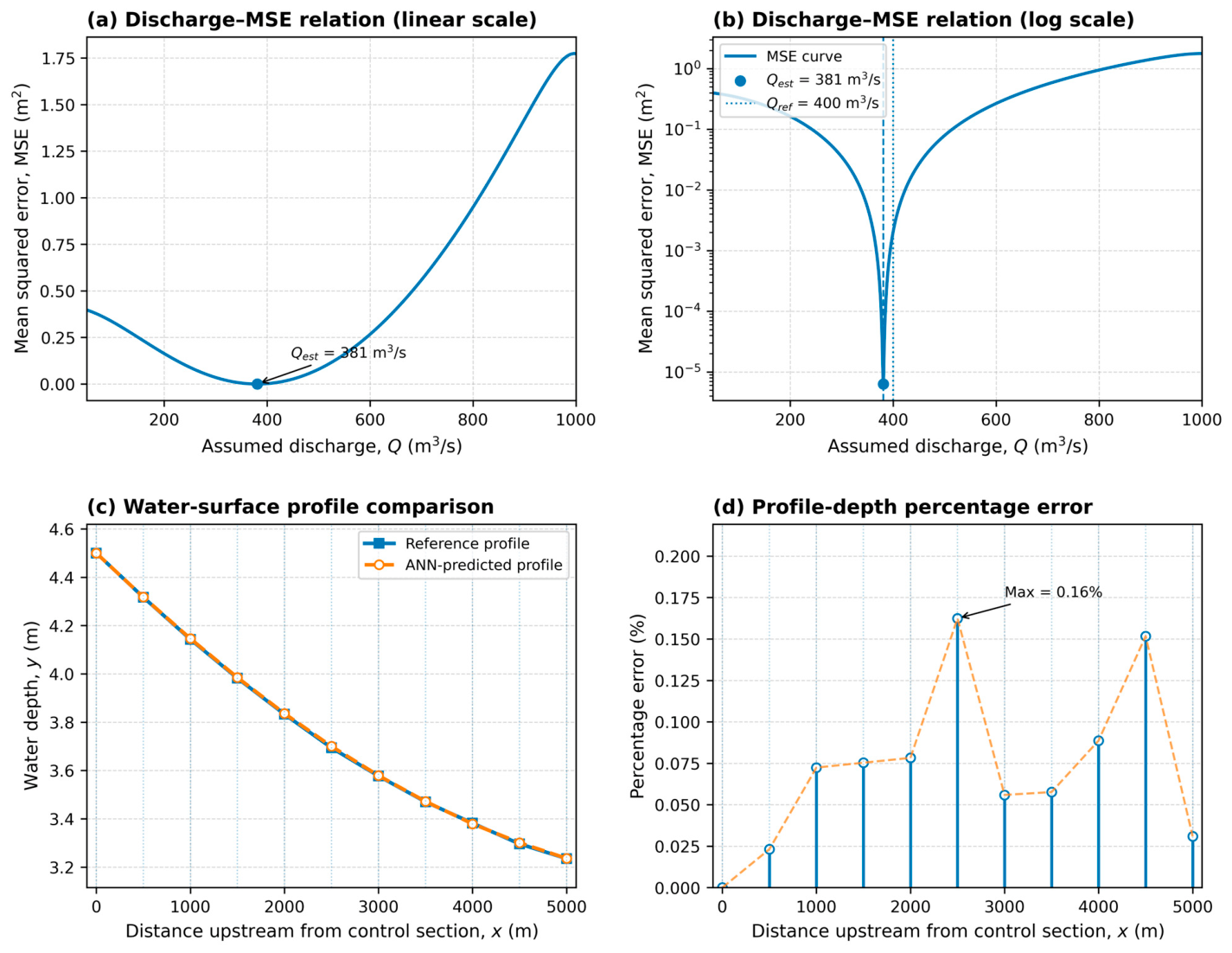
The inverse-discharge results are summarized in Figure 11, which combines the discharge-identification process with the corresponding profile comparison. Figure 11a,b describe the variation of the objective function, expressed as the mean squared error (MSE), with the assumed discharge. Figure 11a presents the discharge–MSE relation using a linear scale, thereby preserving the original visual interpretation of the inverse-search curve, whereas Figure 11b presents the same relation on a logarithmic MSE scale to clarify the minimum-error region. Figure 11c,d then assess the water-surface profile corresponding to the estimated discharge.

Figure 11a shows that the MSE varies systematically with the assumed discharge and exhibits a distinct minimum. This indicates that the longitudinal water-surface profile contains sufficient hydraulic information to identify a most probable discharge within the investigated range. The presence of a well-defined minimum is hydraulically meaningful because it suggests that the inverse problem is not ambiguous over the tested domain. If the profile response were weakly sensitive to discharge, the MSE curve would appear relatively flat and would not support reliable discharge identification.

Figure 11b provides a complementary view of the same inverse-search curve by plotting the MSE on a logarithmic scale. This representation enhances the low-error region and makes the discharge corresponding to the minimum MSE more evident. The discrete search identifies the minimum error at approximately (Q = 381 m³/s), with (MSE = 6.32 × 10⁻⁶ {m²}). A local quadratic interpolation around the minimum gives a very similar estimate of about (Q = 380.83 m³/s), which confirms the stability of the optimum and indicates that the identified minimum is not merely an artifact of the selected discharge increment. When compared with the reference discharge of (400 m³/s), the ANN-based inverse estimate differs by about 4.75%, demonstrating the practical feasibility of the proposed profile-based discharge-estimation approach.

The approximately 4.75% difference between the ANN-inferred discharge and the reference discharge should be interpreted in the context of the uncertainty associated with conventional field measurements of open-channel discharge. For conventional area–velocity measurements using mechanical current meters, Sauer and Meyer [30] reported that the standard error of most individual stream-discharge measurements typically ranges from approximately 3% to 6%, although errors may be as low as about 2% under ideal measurement conditions and can increase substantially under unfavorable hydraulic or field conditions. Comparable uncertainty levels have also been reported for acoustic Doppler current profiler (ADCP) measurements. Morlock [31], based on field comparisons at 12 USGS stream-gauging stations, found that 26 of 31 ADCP discharge measurements differed by less than 5% from discharges determined using conventional methods, while all measurements were within 8%; the corresponding standard deviations generally ranged from approximately 1% to 6%. A subsequent large-scale validation by Oberg and Mueller [32], involving 1032 ADCP transects representing 100 discharge measurements at 22 sites, further demonstrated that properly conducted broadband ADCP measurements were essentially unbiased relative to independent reference-discharge methods. Accordingly, the 4.75% error obtained for the present ANN-based inverse-discharge estimate is of the same order of magnitude as the uncertainty commonly encountered in established field discharge-measurement techniques. The result is therefore considered promising for preliminary hydraulic assessment, operational monitoring, and indirect discharge-estimation applications where direct velocity measurements may be unavailable or impractical. Nevertheless, this level of agreement should not be interpreted as universally acceptable for all engineering purposes, particularly applications requiring high-precision regulatory measurements, calibration-quality discharge data, or water-accounting determinations.

The hydraulic consistency of this estimate is further confirmed by the water-surface-profile comparison in Figure 11c. The ANN-predicted profile closely follows the reference profile along the full reach, indicating that the discharge identified from the MSE minimum produces a physically meaningful longitudinal water-surface variation. The agreement is not limited to a single section near the downstream control, but extends throughout the profile, which is important because inverse discharge estimation depends on matching the overall shape of the water surface rather than reproducing one isolated depth value.

Figure 11d presents the percentage error in water depth along the reach. The errors remain very small at all comparison locations, with a maximum value of about 0.16%. This indicates that the profile predicted using the estimated discharge is almost indistinguishable from the reference profile at the plotted scale. The very small error magnitudes confirm that the minimum identified in the discharge–MSE curve corresponds to a hydraulically informed solution and not merely to a numerical optimum without physical significance.

Taken together, the four panels in Figure 11 show that the ninth ANN model successfully links discharge inference with profile reproduction. Figure 11a,b identify the discharge that minimizes the discrepancy between predicted and reference profiles, whereas Figure 11c,d demonstrate that this discharge reproduces the longitudinal water-surface profile with high accuracy. This result is significant because it extends the ANN framework beyond forward hydraulic prediction and shows that ANN-based surrogates can also support inverse hydraulic analysis.

Nevertheless, the inverse-discharge result remains dependent on the adopted modeling assumptions. The estimated discharge may be affected by uncertainties in the water-depth observations, the spacing of the measurement sections, the channel geometry, Manning’s roughness coefficient, and the downstream boundary condition. Any error in these quantities can alter the shape of the MSE curve and shift the estimated optimum discharge. Therefore, the present result is best interpreted as a proof of concept for ANN-assisted inverse discharge estimation within the investigated hydraulic domain rather than as a universally calibrated field-rating tool.

To quantify these effects more explicitly, a first-order theoretical error-propagation analysis was derived from the GVF equation to relate relative errors in measured water depth to the corresponding uncertainty in the inferred discharge. The analysis further examines the influence of discharge, channel width, Manning’s roughness coefficient, bed slope, and the number and spatial distribution of water-level observation stations. The complete theoretical derivation, dimensionless hydraulic interpretation, and deterministic sensitivity results are presented in Supplementary Section S1 and Figures S1 and S2. The station-configuration results are intended as comparative sensitivity indicators for the investigated hydraulic setting rather than as universal prescriptions for monitoring-network design.

Future research should focus on three main directions. The first is generalization. The GVF and inverse-discharge models should be extended to include variable channel geometry, Manning’s coefficient, bed slope, downstream boundary condition, and cross-section type. The second is physical consistency. Future ANN models may incorporate hydraulic constraints into the training process to enforce monotonicity, conservation-law consistency, and realistic behavior near regime transitions. The third is independent validation. Laboratory experiments and field measurements should be used to test whether the equation-trained models remain reliable under real hydraulic conditions that include uncertainty in roughness, geometry, and water-level observations.

Overall, the present study demonstrates that ANN-based surrogate models can accurately reproduce several important nonlinear open-channel hydraulic calculations when trained within a well-defined hydraulic domain. The scientific value of the study lies not only in the high prediction accuracy but also in the ability of the proposed framework to represent multiple hydraulic principles: resistance balance through Manning’s equation, inertia–gravity balance through critical-depth theory, energy equivalence through alternative depths, momentum conservation through conjugate depths, longitudinal free-surface adjustment through the GVF equation, and profile-based inference through inverse discharge estimation. This multi-process capability supports the potential integration of ANN models into rapid open-channel analysis and design, provided that their assumptions, training ranges, and limitations are clearly stated.

3.5. Observation-Based Natural-River Assessment and Inverse Discharge Estimation (Model 10)

To extend the assessment beyond equation-generated idealized datasets, Model 10 was reformulated as an observation-informed natural-river inverse-discharge application. The case represents the Missouri River at Kansas City, immediately downstream of the Kansas River confluence, using the five cross-sections and hydraulic information reported by Chow [33]. The numerical river representation was reconstructed from the available section geometry and hydraulic properties. Manning’s coefficients of 0.025 for the main channel and 0.050 for the left overbank were adopted where applicable, consistent with the source hydraulic calculations.

A numerical library of 735 steady-flow HEC-RAS profiles was generated to provide broad hydraulic coverage. The simulations combined 35 discharge levels spanning 100–10,000 m³/s with 21 prescribed downstream water-surface elevations spanning 220.0–227.5 m. Because the intended application concerns subcritical gradually varied flow, the resulting profiles were subjected to hydraulic screening. Cases in which HEC-RAS imposed critical depth at one or more sections, together with cases approaching the adopted near-critical threshold, were excluded. This procedure removed 96 profiles and retained 639 fully subcritical numerical realizations. The complete numerical simulation domain adopted hydraulic properties, and profile-screening procedure are documented in Supplementary Section S3.2 and Table S2. These HEC-RAS results are interpreted as a numerical hydraulic baseline and cross-verification dataset rather than independent physical validation.

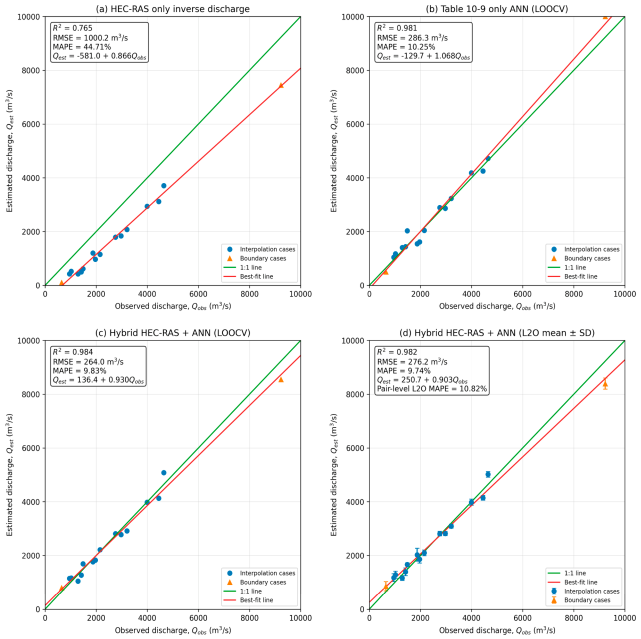
Observation-based assessment was conducted separately using 16 historical stage–discharge events reported by Chow [31], for which discharge and water-surface elevations at Sections 1 and 5 are available. These observations were not simply combined with the substantially larger HEC-RAS dataset because doing so would cause the numerical cases to dominate the limited observation-based information. Instead, four inverse-estimation strategies were compared using the same 16 historical events, as summarized in Figure 12. Further details of the observation-based dataset and the LOOCV and L2O-CV evaluation procedures are provided in Supplementary Sections S3.3 and S3.4, with the corresponding event-wise estimates summarized in Table S3.

In the first approach, the HEC-RAS response surface was inverted directly. For an observed pair and Z_5,obs, discharge was obtained from HEC-RAS generated synthetic data as:

$${\mathrm{Q}}_{\mathrm{H}\mathrm{R}}=\underset{\mathrm{Q}}{\mathrm{a}\mathrm{r}\mathrm{g} \mathrm{m}\mathrm{i}\mathrm{n}}{\left[{\mathrm{Z}}_{5,\mathrm{H}\mathrm{R}}\left(\mathrm{Q},{\mathrm{Z}}_{1,\mathrm{o}\mathrm{b}\mathrm{s}}\right)-{\mathrm{Z}}_{5,\mathrm{o}\mathrm{b}\mathrm{s}}\right]}^2$$

This numerical-model-only estimate resulted in R² = 0.765, RMSE =1000.2 m³/s, and MAPE = 44.71% across the 16 historical events (Figure 12a). The pronounced tendency of the estimated discharges to fall below the 1:1 agreement line indicates a systematic discrepancy between the reconstructed hydraulic model and the historical stage–discharge behavior.

As a second benchmark, the observation-based data [33] were used directly to develop a compact ANN mapping

$$\left(\mathrm{Q},{\mathrm{Z}}_1\right)\to {\mathrm{Z}}_5,$$

Because only 16 observations were available, performance was evaluated using leave-one-out cross-validation (LOOCV) rather than a single random train–validation–test partition. In every LOOCV run, the tested observation was omitted completely from development of the ANN used to estimate that event. The forward ANN was subsequently inverted by varying discharge until the predicted Section-5 water level matched the observed value. This observation-only ANN produced R² = 0.981, RMSE = 286.3 m³/s, and MAPE = 10.25% across the 16 withheld events (Figure 12b). For the 14 interior observations that remained within the discharge envelope of the corresponding development datasets, the MAPE and RMSE were 9.48% and 223.4 m³/s, respectively.

A third assessment combined the hydraulic baseline with an observation-informed ANN discrepancy correction. The HEC-RAS inverse estimate was first obtained for each observed stage pair. A compact regularized correction ANN then estimated the residual

$$\mathsf{\Delta }\mathrm{Q}={\mathrm{Q}}_{\mathrm{o}\mathrm{b}\mathrm{s}}-{\mathrm{Q}}_{\mathrm{H}\mathrm{R}},$$

and the final discharge was calculated as

$${\mathrm{Q}}_{\mathrm{h}\mathrm{y}\mathrm{b}\mathrm{r}\mathrm{i}\mathrm{d}}={\mathrm{Q}}_{\mathrm{H}\mathrm{R}}+\mathsf{\Delta }{\mathrm{Q}}_{\mathrm{A}\mathrm{N}\mathrm{N}}.$$

Under strict LOOCV, the hybrid formulation yielded R² = 0.984, RMSE = 264.0 m³/s, and MAPE = 9.83% for all 16 events (Figure 12c). For the 14 interpolation events, For the 14 interpolation events, MAPE decreased to 9.10%, with an RMSE of 212.3 m³/s. Relative to the observation-only ANN benchmark, the hybrid formulation therefore reduced the overall RMSE by approximately 7.8%, indicating that the hydraulic baseline provides useful additional information even though the field correction remains necessary.

Robustness to the limited observation-based sample size was further examined using exhaustive leave-two-out cross-validation. All 120 possible pairs of observations were withheld in turn, so that every correction model was developed from only 14 field events. Each observation consequently received 15 independent estimates, corresponding to the 15 possible companion observations removed with it. Figure 12d presents the mean estimate for each event together with its ±1 standard deviation range. The mean-per-event predictions yielded R² = 0.982, RMSE = 276.2 m³/s, and MAPE = 9.74%. Across the complete set of 240 individual leave-two-out predictions, MAPE and RMSE were approximately 10.82% and 304.6 m³/s, respectively. The modest deterioration relative to LOOCV is consistent with the reduction of the observation-based development set from 15 to 14 events and provides an additional indication that the inferred relationship is not dependent on a single favorable data partition.

The four panels in Figure 12 therefore separate numerical hydraulic fidelity from observation-based predictive assessment. HEC-RAS alone does not reproduce the historical stage–discharge relationship sufficiently accurately, whereas the observation-informed approaches move the predictions markedly closer to the 1:1 line. The hybrid formulation provides a modest but consistent improvement over the ANN developed from the historical observations alone and, more importantly, establishes a structured mechanism by which a physics-based numerical baseline can be corrected using limited site-specific observations. A consolidated comparison of the corresponding performance statistics is provided in Supplementary Table S3, while the complete simulation matrix, hydraulic screening criteria, event-wise estimates, and cross-validation results are documented in Supplementary Section S3. A consolidated comparison of the numerical and observation-informed performance statistics is provided in Supplementary Table S4, while the numerical simulation domain and hydraulic screening, observation-based dataset, event-wise estimates, and LOOCV/L2O-CV procedures are documented in Supplementary Section S3 and Tables S3 and S4. This result should nevertheless be interpreted as an observation-based proof of concept for the investigated historical reach rather than as universal field validation.

3.6. Integrated Example Using Developed ANN Models

To demonstrate the coordinated use of the developed ANN surrogates within practical hydraulic calculations, two representative gate-controlled channel problems were examined. Unlike the individual model assessments presented in the preceding sections, these examples employ several ANN modules within the same hydraulic problem. The objective is therefore to illustrate how independently trained surrogate models representing different hydraulic principles can be used collectively within a conventional open-channel analysis workflow.

3.6.1. Example 1: Mild-Slope Gate-Controlled Reach

The first example considers a trapezoidal channel with a Manning roughness coefficient of n = 0.025, bed slope So = 0.0005, bed width b = 8 m, side slope t = 2H:1V, and discharge Q = 30 m³/s, Figure 13. A gate with an opening of 0.4 m and a contraction coefficient Cc = 0.65 is located within the reach. The required hydraulic quantities include the normal depth, critical depth, upstream gate-related depth, and the downstream conjugate depth associated with a hydraulic jump immediately downstream of the gate.

The corresponding ANN surrogates were applied to determine the relevant hydraulic depths, and the predictions were compared with values obtained from the conventional governing equations. The results are summarized in

Table 5. Comparison of ANN predictions and conventional hydraulic solutions for Example 1.

Method	(yo) (m)	(yc) (m)	(y2_alt) (m)	(y2_conj) (m)
ANN surrogates	2.113	1.030	9.615	2.609
Used ANN No.	1	3	5	6
Conventional equations	2.112	1.030	9.607	2.608

. The ANN predictions show very close agreement with the conventional solutions.

These results demonstrate that several surrogate modules can be employed within a single hydraulic problem to reproduce resistance-controlled normal flow, inertia–gravity-controlled critical flow, specific-energy-based alternative depth, and momentum-controlled conjugate depth with negligible loss of accuracy relative to the corresponding conventional calculations.

3.6.2. Example 2: Steep-Slope Reach with Hydraulic Jump and Downstream Gate Control

The second example considers a trapezoidal channel having the same bed width, side slope, Manning coefficient, and discharge as Example 1, but with a substantially steeper bed slope of So = 0.01, gate opening of 0.691 m and a contraction coefficient Cc = 0.65, Figure 14. Under these conditions, the normal flow is supercritical. A downstream gate imposes a subcritical control, and a hydraulic jump is assumed to occur 200 m upstream of the gate. The analysis requires determination of the normal depth, critical depth, conjugate depth, upstream gate depth, and the resulting S1 water-surface profile between the hydraulic jump and the gate.

The ANN-based results were compared with HEC-RAS numerical cross-verification solution,

Table 6. Comparison of ANN and HEC-RAS hydraulic depths for Example 2.

Method	(yo) (m)	(yc) (m)	(y2_alt) (m)	(y2_conj) (m)	(y_gate) (m)
ANN surrogates	0.923	1.030	3.303	1.144	3.298
Used ANN model No.	1	3	5	6	8
HEC-RAS	0.923	1.030	3.302	1.144	3.302

. The predicted gate depth was 3.298 m compared with 3.302 m from HEC-RAS, corresponding to an absolute difference of 0.004 m, or approximately 0.12%.

The longitudinal water-surface profile provides a more detailed assessment of the integrated calculation. Over the 200 m reach between the hydraulic jump and the downstream gate, the ANN-generated profile follows the HEC-RAS solution closely,

Table 7. Comparison of the ANN 8 - and HEC-RAS-predicted S1 water-surface profiles for Example 2.

Distance from Gate, (L) (m)	200	175	150	125	100	75	50	25	0
ANN depth (m)	1.144	1.450	1.737	2.012	2.278	2.537	2.793	3.046	3.298
HEC-RAS depth (m)	1.144	1.479	1.758	2.024	2.284	2.540	2.795	3.048	3.302
Error (%)	0%	2%	1%	1%	0%	0%	0%	0%	0%

. The pointwise percentage differences along the 200 m reach range from approximately 0% to 2%, with no systematic increase or decrease in error toward either boundary. Together with the approximately 0.12% difference in gate depth, this close agreement demonstrates that Model 8 can reproduce both the principal hydraulic depths and the longitudinal development of the downstream-controlled S1 profile for the investigated case.

Taken together, the two examples demonstrate the coordinated application of multiple ANN surrogate modules within complete hydraulic calculation sequences. These examples therefore complement the individual model-validation results by illustrating how the modular ANN framework can support multi-step open-channel hydraulic analyses while maintaining close agreement with conventional equations and HEC-RAS simulations.

4. Conclusions

This study developed and evaluated a hydraulically informed ANN surrogate framework for a coordinated sequence of nonlinear open-channel hydraulic calculations. The framework comprises independently trained surrogate modules for normal and critical depths in trapezoidal and circular sections, alternative and conjugate depths, gradually varied flow (GVF) under mild- and steep-slope conditions, water-surface-profile mapping, and inverse discharge estimation. The contribution is therefore not the introduction of new hydraulic equations or a fundamentally new neural-network architecture. Rather, it is a framework-level contribution in which established hydraulic relationships are formulated as compatible, rapidly evaluated surrogate mappings that can be used individually or coordinated within forward, inverse, sensitivity, and optimization workflows. Hydraulic information is introduced through physically meaningful and, where appropriate, dimensionless variables, hydraulic applicability domains, and reference solutions generated from governing equations or numerical hydraulic models. The ANN optimization itself remains data driven; therefore, the proposed models are hydraulically informed surrogates rather than physics-informed neural networks and do not inherently enforce conservation, monotonicity, positivity, or physically admissible extrapolation outside the represented domains.

The forward ANN models reproduced the corresponding deterministic hydraulic solutions with high accuracy within the investigated parameter ranges. Models 1–4 captured the nonlinear relationships governing normal and critical depths, Models 5 and 6 represented energy- and momentum-controlled transition depths, and Models 7 and 8 extended the framework to spatial free-surface behavior governed by the GVF equation. The M1 and S1 profile comparisons with HEC-RAS showed close agreement in longitudinal water-surface variation; however, these comparisons are interpreted as numerical hydraulic cross-verification rather than independent physical validation, because both modeling approaches ultimately rely on established hydraulic governing principles. The integrated mild- and steep-slope examples further demonstrated that independently trained surrogate modules can be combined within multi-step hydraulic calculation sequences while retaining close agreement with conventional hydraulic solutions, without implying joint training or a fully cascaded end-to-end ANN architecture.

The expanded comparison with alternative surrogate methods further clarified the rationale for ANN selection. ANN, Random Forest, support vector regression with a radial-basis-function kernel, and Gaussian Process Regression were systematically compared for three hydraulically distinct mappings represented by Models 1, 5, and 7. The results did not indicate universal superiority of ANN under every error metric. For the smooth Model 1 mapping, several methods achieved very high accuracy, while GPR produced a slightly smaller absolute RMSE than ANN. For the strongly nonlinear Model 5 alternative-depth problem, ANN provided the strongest overall predictive performance, with a MAPE of approximately 0.775% compared with 3.155% for GPR and larger errors for RF and SVR. For Model 7, GPR achieved a modest advantage in absolute error, with R² = 0.8873 and RMSE = 0.4633 compared with R² = 0.8615 and RMSE = 0.5136 for ANN, whereas ANN produced substantially lower relative error, with a MAPE of 1.058% compared with 2.480% for GPR. Taken together with the compact fixed-size ANN representation and low post-training inference cost, these results support ANN as a favorable accuracy–complexity–inference-efficiency compromise for the repeated-evaluation applications targeted in this study rather than as an intrinsically optimal learning algorithm.

The computational assessment similarly showed that surrogate efficiency must be evaluated beyond post-training inference alone. For Models 5–8, ANN inference provided substantial acceleration relative to the corresponding conventional iterative or numerical procedures, with the largest gain occurring for the mild-slope GVF problem because conventional evaluation requires repeated integration of the governing differential equation. However, dataset generation and network training constitute non-negligible one-time development costs. The accompanying break-even analysis therefore provides a more realistic measure of computational benefit by identifying the number of repeated evaluations required to recover this initial investment. For Model 7, for example, the approximately 249-fold post-training acceleration offsets the model-development cost after approximately 1.03 × 10⁵ evaluations. The practical computational advantage of the surrogate approach is consequently greatest in high-throughput applications such as sensitivity analysis, uncertainty propagation, optimization, inverse estimation, Monte Carlo simulation, and repeated operational assessment rather than in isolated one-off calculations.

Model 9 extended the framework from forward prediction to inverse hydraulic analysis by inferring discharge from a spatial water-surface profile. The estimated discharge of approximately 381 m³/s, compared with the 400 m³/s reference value, corresponds to an error of approximately 4.75%. This level of agreement is promising but should not be interpreted as universally acceptable for all engineering applications. Its magnitude is of the same order as the uncertainty commonly encountered in conventional field discharge measurements and may therefore be useful for preliminary hydraulic assessment, operational monitoring, and situations in which direct discharge measurement is difficult. Nevertheless, applications requiring calibration-quality, regulatory, or water-accounting accuracy may require substantially tighter uncertainty bounds. The associated theoretical and numerical sensitivity analyses further demonstrated that inverse-discharge reliability depends on water-level measurement error, flow state, channel geometry, Manning’s roughness, bed slope, and the number and spatial arrangement of observation stations. Accordingly, Model 9 should be regarded as a proof of concept for ANN-assisted profile-based discharge inference rather than as a replacement for established field measurement procedures.

Model 10 provided a more stringent observation-based natural-river assessment using 16 historical stage–discharge events for the Missouri River at Kansas City. The revised analysis deliberately separated the HEC-RAS numerical hydraulic baseline from the observation-based information. Direct inversion of the reconstructed HEC-RAS response surface produced R² = 0.765, RMSE = 1000.2 m³/s, and MAPE = 44.71%, demonstrating that the numerical model alone did not reproduce the historical stage–discharge relationship adequately. In contrast, the observation-only ANN evaluated through leave-one-out cross-validation produced R² = 0.981, RMSE = 286.3 m³/s, and MAPE = 10.25%. The hybrid HEC-RAS–ANN discrepancy-correction formulation further improved the overall performance to R² = 0.984, RMSE = 264.0 m³/s, and MAPE = 9.83%. Exhaustive leave-two-out testing yielded a MAPE of approximately 10.82% and RMSE of approximately 304.6 m³/s across the complete set of 240 withheld predictions. These results demonstrate that the ANN component is not merely reproducing the numerical HEC-RAS solution; rather, observation-based information can be used to correct systematic site-specific discrepancies in the numerical hydraulic baseline. Nevertheless, because the assessment is based on only 16 historical observation-based events from a single reach, Model 10 should be interpreted as an observation-based proof of concept rather than comprehensive field validation.

Several limitations therefore remain fundamental to the interpretation of the results. Most forward surrogates were developed from equation- or numerically generated datasets, so their high test accuracy primarily establishes fidelity to the corresponding deterministic hydraulic mappings within the represented domains. Reliable extrapolation outside those domains is not established. The current framework also does not comprehensively represent arbitrary irregular or compound geometry, spatially variable roughness, vegetation, sediment transport, strongly turbulent local phenomena, or unsteady flow. In addition, the individual ANN modules are independently trained, and cumulative error propagation in a fully cascaded ANN-to-ANN implementation has not yet been quantified. The architecture sensitivity assessment supports the retained two-hidden-layer, 15-neuron configuration for Model 1 among the tested candidates, but it does not establish that this architecture is globally optimal for every model within the framework.

Future work should consequently focus on broader independent observation-based assessment across additional rivers, laboratory experiments, hydraulic regimes, and contemporary field datasets; extension to irregular and compound geometries, spatially varying roughness, additional boundary conditions, and unsteady flow; and development of physics-constrained surrogates incorporating conservation residuals, monotonicity, positivity, or other hydraulic admissibility conditions. Further investigation of uncertainty propagation in cascaded surrogate workflows, transfer learning using limited site-specific observations, and probabilistic formulations for prediction uncertainty would also strengthen practical deployment.