Discharge Simulation Evaluations of ISIMIP3a Global Hydrological Models in the Yangtze River Basin

Abstract

Global hydrological models (GHMs) are essential for assessing water resources and flood risk, yet systematic evaluations of ISIMIP3a models remain limited. We evaluated eight standard ISIMIP3a GHM configurations against observed discharge at four principal Yangtze mainstem gauges using a multi-metric framework covering daily and monthly discharge, the seasonal cycle (defined as the mean annual cycle of monthly discharge), flow percentiles, and annual peak discharge. Metric-based model performance generally increased from daily to monthly and seasonal-cycle scales, partly reflecting the smoothing of short-term errors through temporal aggregation, whereas annual peak discharge remained more difficult to reproduce. WaterGAP2-2e achieved the strongest overall performance across the daily, monthly, and seasonal-cycle evaluations. However, this result was not fully independent of its inherited global discharge calibration, because three evaluation gauges (Yichang, Hankou, and Datong) spatially coincide with gauges in its calibration-station dataset. WaterGAP2-2e also systematically overestimated peak flows, with peak-flow Relative Bias (RBpeak) reaching 30.14%. Among the remaining configurations, WEB-DHM-SG showed the strongest overall performance and a relatively small station-averaged absolute peak-flow bias (|RB_peak| = 15.52%). However, this advantage did not extend to low-flow conditions. H08 and ORCHIDEE-MICT showed the weakest overall performance, with negative NSE values down to −3.61 and peak-flow biases reaching −99.10%, whereas MIROC-INTEG-LAND, CWatM, HydroPy, and JULES-W2-DDM30 showed intermediate performance. Overall, model suitability depended on temporal scale and flow regime, and apparent rankings should be interpreted in light of inherited calibration and configuration differences. These results provide a diagnostic basis for model selection and targeted improvement in regional discharge simulation and peak-flow-related applications.

1. Introduction

Global hydrological models (GHMs) play a crucial role in evaluating climate change impacts on hydrological processes [1,2]. The societal relevance of reliable hydrological assessment is increasing as climate change is projected to expose future generations to unprecedented river-flood conditions and to amplify the economic consequences of climate extremes [3,4]. The Inter-Sectoral Impact Model Intercomparison Project (ISIMIP) has pioneered an innovative framework for GHM simulations by integrating multidisciplinary models with standardized multi-scenario datasets [5,6]. The recent ISIMIP3a water-sector ensemble provides standardized GHM simulations under a common forcing and output framework [5,7], creating a consistent basis for model intercomparison. However, the standard configurations retain differences in inherited calibration, routing schemes, and human–water representations [5,8], making regional benchmark evaluations necessary to identify model-specific strengths and limitations.

International GHM intercomparison studies have shown that model performance varies substantially across models, regions, temporal scales, and flow regimes [8,9]. A recent evaluation of eight global water models further showed that discharge performance varies across geographic and climatic regions and can deteriorate as human impacts intensify [8]. Using multi-model validation, Veldkamp et al. [9] showed that human-impact parameterizations can improve estimates of monthly discharge and hydrological extremes, while other studies emphasized the importance of regionalization and parameter estimation when transferring GHMs to basin-scale applications [10,11]. Nevertheless, systematic discharge biases remain at the global scale [12], and flood simulations continue to show substantial uncertainty [13,14]. These findings indicate that GHM performance should be assessed using multiple metrics, temporal scales, and flow conditions rather than a single aggregate measure.

The Yangtze River Basin is a strategic hydrological region with major socioeconomic importance in China and is strongly affected by climate variability and intensive human activities [15,16,17,18]. Previous Yangtze-focused studies have examined runoff responses to extreme precipitation [19], reservoir-induced changes in streamflow [16], and climate change impacts on discharge [18]. More recently, Zhao et al. [20] demonstrated that basin-specific calibration can improve regional flood- and drought-related simulations of a global hydrological model. Such work highlights the value of regional calibration for basin-scale applications but does not show how multiple standard GHM configurations, used without additional Yangtze-specific recalibration, compare under a common evaluation framework. Gauge-based multi-model benchmarking of standard ISIMIP3a configurations at major Yangtze mainstem stations therefore remains limited [8,12,20].

Here, we evaluate eight standard ISIMIP3a GHM configurations at four principal Yangtze mainstem gauges under common forcing and a consistent output framework. Using complementary metrics, the analysis addresses three diagnostic questions: (1) whether model skill and relative ranking remain consistent across daily discharge, monthly discharge, the seasonal cycle (i.e., the mean annual cycle of monthly discharge), and annual peak discharge; (2) whether models that reproduce overall discharge dynamics also reproduce low-flow percentiles and annual peak discharge; and (3) how inherited calibration and model-configuration differences constrain the interpretation of apparent model skill. By integrating these diagnostics, the study identifies cross-scale and flow-regime-specific strengths and weaknesses that would be obscured by a single aggregate ranking.

2. Materials and Methods

2.1. The Yangtze River

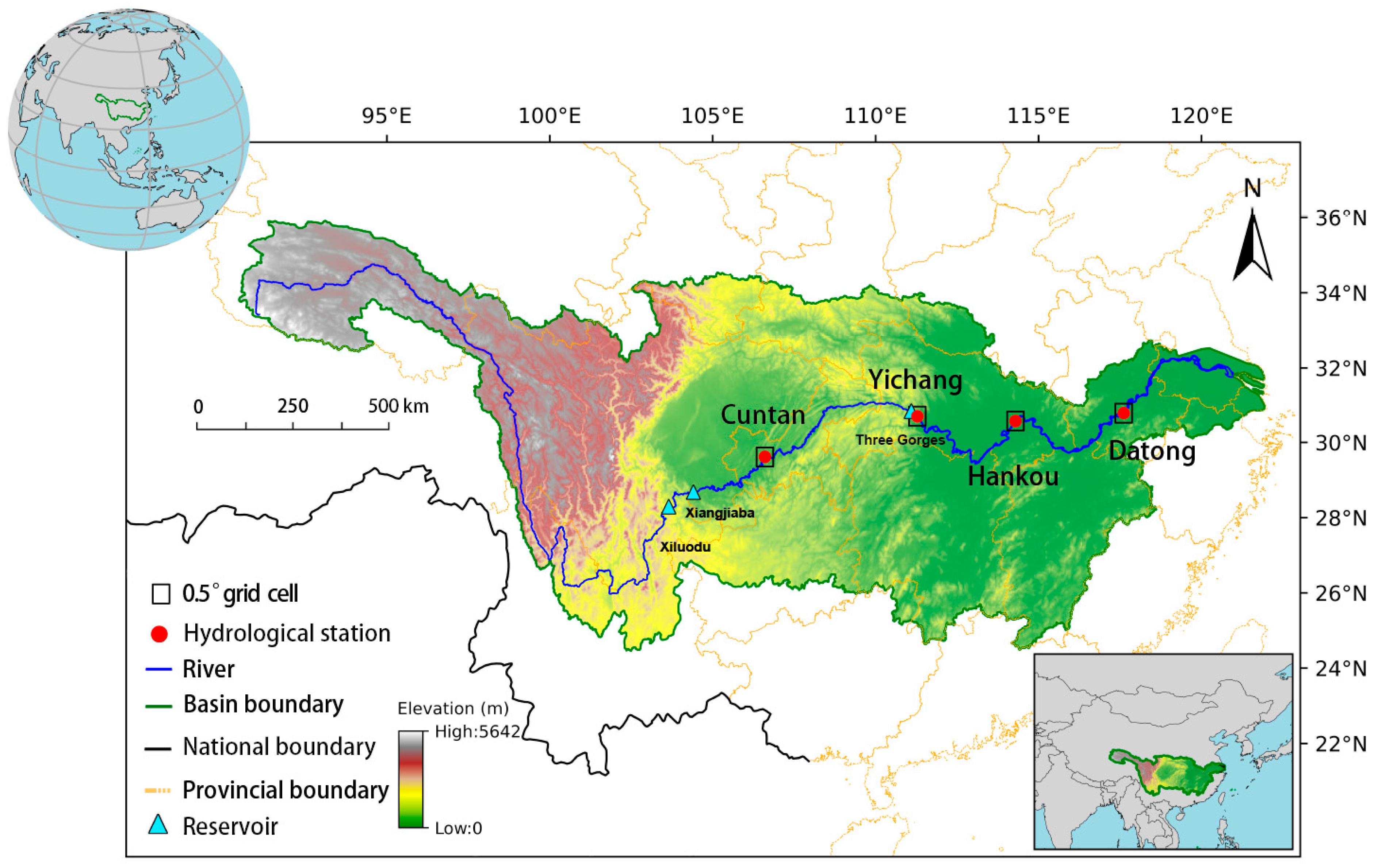
The Yangtze River Basin (24°30′–35°45′ N, 90°33′–122°25′ E), China’s largest river system, spans approximately 1.8 million km² and delivers a mean annual runoff volume of approximately 960 billion m³ [21,22]. The basin experiences a subtropical monsoon climate marked by pronounced spatiotemporal variability in precipitation, driving diverse hydrological regimes across its upper, middle, and lower reaches [21,23]. The locations of the Yangtze River Basin and the four gauging stations are shown in Figure 1.

2.2. Datasets

Eight GHM simulations from the historical ISIMIP3a water-sector simulations were used as the model discharge data [5]. All simulations were driven by the same daily GSWP3-W5E5 meteorological forcing [5,7], comprising precipitation, 2 m air temperature, shortwave and longwave radiation, specific humidity, surface pressure, and near-surface wind speed on a 0.5° × 0.5° latitude–longitude grid. The evaluated output was daily river discharge (dis), expressed in m³ s⁻¹ [5]. Examination of the original NetCDF metadata showed that all eight discharge outputs were stored as dis (time, lat, lon) on a regular global grid comprising 360 latitude and 720 longitude cells, with coordinates representing grid-cell centers, and used the proleptic Gregorian calendar.

Observed daily discharge records at four principal Yangtze River gauging stations were used as the reference data for model evaluation. The four stations are Cuntan, Yichang, Hankou, and Datong, representing the upper reach, the upper-middle transition, the middle reach, and the lower reach of the Yangtze River, respectively. These stations were selected as major mainstem gauges to evaluate integrated discharge responses along the upper-to-lower Yangtze River. The evaluation therefore focuses on integrated mainstem discharge responses rather than separate tributary or sub-basin-scale responses. The reference discharge records were derived from in situ measurements at the four gauging stations; thus, model performance was evaluated against observations rather than against another simulation product. Detailed metadata on the administering agency/database and station-level quality-control procedures were unavailable in the records accessible for this study; therefore, no unverified provenance or quality-control information was inferred. The observed discharge records represent the observed river-flow conditions during the respective evaluation periods, including any effects of reservoir operations present in the measured flows.

The available evaluation periods were determined by the overlap between observed discharge records and GHM simulations: Cuntan, 1975–2008; Yichang, 1950–2002; Hankou, 1976–2001; and Datong, 1976–2001. The unequal record lengths reflect differences in the availability of continuous in situ observations. The records from the three downstream gauges end in 2002, whereas the longer Cuntan record is from a station upstream of the Three Gorges Reservoir.

2.3. Global Hydrological Models

WEB-DHM-SG is a previously developed hydrological–hydrodynamic coupled model and was not newly developed in this study [24,25]. The model has been described in previous work, and its routing representation builds on the CaMa-Flood framework [26]. The WaterGAP2-2e model integrates natural hydrological cycles with anthropogenic water use—including irrigation, industrial consumption, and reservoir operations—to simulate global water resource dynamics [27]. The H08 model, an integrated water resource management framework, incorporates irrigation demand, reservoir operations, and groundwater abstraction [28].

The CWatM model employs a modular architecture that integrates surface and groundwater hydrological processes with human water use, reservoir regulation, water demand, and return flows [29,30]. The HydroPy model, a global distributed hydrological framework, simulates large-scale basin hydrological cycles by integrating physical mechanisms with spatially heterogeneous drivers such as topography, vegetation, and soil properties [31]. The JULES-W2-DDM30 model is based on the Joint UK Land Environment Simulator (JULES), which couples vegetation and hydrological processes, with DDM30 used as the river-routing network [32,33,34]. MIROC-INTEG-LAND is an integrated land model that couples water resources, crop production, ecosystem processes, and land-use change [35]. ORCHIDEE-MICT extends the ORCHIDEE land-surface framework with high-latitude process representations that describe interactions among soil carbon, soil temperature, and hydrology and their feedbacks on water and CO₂ fluxes [36]; the evaluated ISIMIP3a water-sector configuration is documented by ISIMIP [37].

Taken together, the eight GHMs differ substantially in their routing schemes and representations of human water use and reservoirs [25,30,33,37,38,39,40,41]. Among the evaluated configurations, only WEB-DHM-SG incorporates the modified CaMa-Flood hydrodynamic routing module based on DDM30 [25], whereas the other models use different routing schemes or river-network formulations [30,33,37,38,39,40,41]. Reservoir operations and human–water processes were not harmonized separately in this study but were retained as specified in each model’s standard ISIMIP3a configuration [5,25,30,33,37,38,39,40,41]. These structural and configuration differences provide important context for interpreting inter-model performance. Detailed routing schemes, human-water-use sectors, and reservoir representations are provided in Table S1 [42].

All eight GHM simulations were evaluated as provided in the ISIMIP3a ensemble [5], and no model was recalibrated against the four Yangtze River gauges in this study, because the objective was to benchmark the standard ISIMIP3a configurations under a common forcing framework. WaterGAP2-2e was globally calibrated by its development team against observed river discharge, with the Global Runoff Data Centre (GRDC) serving as the main source of streamflow gauging-station data [27,43]. Based on the coordinates of the WaterGAP2-2e global calibration gauges, the calibration-station dataset was spatially screened using the Yangtze River Basin boundary, identifying eight calibration gauges within the basin. The identities and locations of these gauges were then compared with the four evaluation gauges, showing that Yichang, Hankou, and Datong overlap with the WaterGAP2-2e calibration dataset, whereas Cuntan does not. H08 retained the climate-zone-specific parameter optimization following Yoshida et al. (2022) [44]. The remaining models were evaluated using their standard ISIMIP3a configurations without additional Yangtze-specific calibration or optimization [5]. Accordingly, no Yangtze-specific parameter ranges or optimal parameter values were estimated in this study.

Table 1. Summary of the eight ISIMIP3a global hydrological models evaluated in this study.

Model	Key ISIMIP3a Characteristics	Calibration/ Parameter Setting
WEB-DHM-SG	Distributed biosphere hydrological model with improved snow physics and modified CaMa-Flood routing based on DDM30 [25].	Not calibrated
WaterGAP2-2e	Global water resources and use model with linear-reservoir routing and water resources representation [38].	Calibrated against observed river discharge
H08	Integrated global water resources model with TRIP/DDM30 routing and water management representation [39].	Climate-zone parameter optimization
CWatM	Community Water Model with 3 soil layers, kinematic-wave routing, and dynamic water demand [30].	Not calibrated
HydroPy	Global hydrological model combining land-surface hydrological processes and river routing [40].	Not calibrated
JULES-W2-DDM30	JULES-W2 simulations using DDM30 as the river-routing network [33].	Not calibrated
MIROC-INTEG-LAND	Integrated land model coupling water resources, crop production, ecosystem, and land-use modules [41].	Not calibrated
ORCHIDEE-MICT	ISIMIP3a water-sector model; detailed structural information is limited on the ISIMIP3a model page [37].	Not specified on ISIMIP3a page

Note. This table summarizes the main characteristics needed to differentiate the eight models in the main text. More detailed configuration information is provided in Table S1. For H08, calibration refers to climate-zone parameter optimization reported in the ISIMIP3a documentation, not basin-specific discharge calibration for the Yangtze gauges in this study. “Not specified” indicates that calibration or parameter-setting information was unavailable on the corresponding ISIMIP3a model page and should not be interpreted as evidence that the model was uncalibrated. Detailed routing, human-water-use, and reservoir configurations are provided in Table S1.

, therefore, summarizes the key ISIMIP3a characteristics and calibration or parameter-setting status of the eight GHMs rather than basin-specific optimization results.

2.4. Data Processing and Evaluation Design

To make full use of the available observational information, each gauge was evaluated over its complete available record rather than restricting all four gauges to their common overlapping period. At each gauge, all eight GHMs were evaluated over the same station-specific period, ensuring temporally consistent within-gauge comparisons. Consequently, the gauge-level evaluations correspond to different historical periods across the four stations. To assess the sensitivity of the cross-gauge summary metrics to the unequal historical evaluation windows, a supplementary common-period analysis was conducted for 1976–2001, which is shared by all four gauges. Daily, monthly, seasonal-cycle, and annual peak-discharge metrics were recalculated using the same data-processing and metric calculation procedures as in the primary analysis. Cross-gauge averages were calculated using the same unweighted averaging procedure, with absolute gauge-level RB and RBpeak values averaged for the bias-based summaries. The common-period results were compared with the primary station-specific full-record results to assess the robustness of the cross-model patterns.

ISIMIP3 provides the DDM30 river-routing network as a standardized global drainage-direction dataset for water-sector simulations [45,46]. DDM30 represents surface-water drainage directions at 30′ spatial resolution and has been extensively validated and applied in large-scale global hydrological studies [45,47]. All four gauges are located along the Yangtze River mainstem. For each gauge, the corresponding 0.5° × 0.5° model grid cell was identified using the gauge coordinates together with the mapped alignment of the Yangtze mainstem. No automated river-network snapping algorithm was applied. Because all eight GHM discharge outputs share the same spatial grid, the same station-to-grid assignments were applied consistently across all models. Simulated discharge was extracted from the selected grid cells, whose spatial extents are shown in Figure 1. The observed gauge coordinates and corresponding model grid-cell center coordinates are provided in Table S23. The observed and simulated daily discharge series were aligned by calendar date without lag optimization or temporal shifting. In the data-processing procedure, discharge values coded as −999 and dates without available observations were represented as missing values (NaN). Model performance metrics were calculated only from paired observed and simulated values after excluding dates with missing values in either series. The upstream drainage areas represented by the selected model grid cells were not quantitatively matched to the reported drainage areas of the corresponding gauges.

Monthly discharge series were derived from the aligned daily series by calculating the monthly mean discharge. The seasonal cycle was subsequently obtained by averaging the monthly discharge values for each calendar month across all years within the corresponding station-specific evaluation period. Thus, both the monthly and seasonal-cycle evaluations were derived from the original daily discharge series rather than from independent monthly model simulations. Annual peak discharge was defined as the maximum daily discharge within each calendar year and was used for the subsequent peak-flow magnitude and trend analyses.

2.5. Evaluation Metrics

This study used a multi-metric framework to evaluate the performance of the eight GHMs across daily discharge, monthly discharge, the seasonal cycle, different parts of the discharge distribution, and annual peak discharge. Daily discharge was evaluated using Nash–Sutcliffe Efficiency (NSE), Relative Bias (RB), Pearson’s correlation coefficient (R), and mean absolute error (MAE), whereas monthly discharge and the seasonal cycle were evaluated using NSE, R, and MAE. Flow-percentile performance was assessed using percentile-specific RB, and annual peak-discharge magnitude was assessed using the Relative Bias of peak flow (RB_peak). For each metric, the station-averaged value was calculated as the unweighted arithmetic mean of the corresponding gauge-level values across the four gauges, with each gauge-level value derived from its station-specific evaluation period. For bias-based cross-gauge summaries, the absolute gauge-level RB or RB_peak values were averaged to avoid cancellation between positive and negative biases. These averages provide only a descriptive cross-gauge summary of model performance and should not be interpreted as rankings based on a common historical period or as area-weighted basin-wide hydrological averages.

NSE quantifies the goodness of fit between simulated and observed discharge and is widely used for hydrological model evaluation [48]. It is defined as follows:

$$NSE=1-{\displaystyle \frac{{\displaystyle \sum {(Q_{obs}-Q_{sim})}^2}}{{\displaystyle \sum {(Q_{obs}-\overline{Q_{obs}})}^2}}}$$

(1)

where $Q_{obs}$ denotes the observed values, $Q_{sim}$ represents the simulated values, and $\overline{Q_{obs}}$ is the mean of the observed values. RB measures volumetric errors and systematic deviations in long-term discharge-volume bias:

$$RB={\displaystyle \frac{{\displaystyle \sum Q_{sim}-{\displaystyle \sum Q_{obs}}}}{{\displaystyle \sum Q_{obs}}}}\times 100\%$$

(2)

R measures the temporal correspondence between simulated and observed discharge series [49]:

$$R={\displaystyle \frac{{\displaystyle \sum \left(Q_{obs}-\overline{Q_{obs}}\right)\left(Q_{sim}-\overline{Q_{sim}}\right)}}{\sqrt{{{\displaystyle \sum \left(Q_{obs}-\overline{Q_{obs}}\right)}}^2}\sqrt{{{\displaystyle \sum \left(Q_{sim}-\overline{Q_{sim}}\right)}}^2}}}$$

(3)

where $\overline{Q_{sim}}$ is the mean of the simulated values. MAE was used to quantify the mean absolute magnitude of simulation errors, with the same unit as discharge [50]:

$$MAE={\displaystyle \frac{1}{n}}\mid {\displaystyle \sum _{i=1}^n\left|Q_{sim,i}-Q_{obs,i}\right|}$$

(4)

where $Q_{obs,i}$ and $Q_{sim,i}$ denote the observed and simulated discharge values at time step $i$, respectively, and $n$ is the number of valid paired observations.

Taylor diagrams were also used as a complementary diagnostic to jointly summarize the Pearson correlation coefficient, R, the normalized standard deviation, and the centered root-mean-square difference between simulated and observed discharge [51]. The Taylor diagrams were constructed from the same temporally aligned or aggregated observed and simulated discharge series used for the corresponding scale-specific evaluations. Kling–Gupta efficiency (KGE) was not additionally calculated because its principal diagnostic dimensions—correlation, bias, and variability—were examined separately using R, RB, and the Taylor-diagram diagnostics [52].

To evaluate model performance across different parts of the discharge distribution, flow-percentile diagnostics were calculated from daily discharge series. The 5th, 10th, 25th, 50th, and 95th percentiles were used to represent low-flow to high-flow conditions. The Relative Bias for each percentile was calculated as follows:

$$R{B}_{Q_p}={\displaystyle \frac{Q_{p,sim}-Q_{p,obs}}{Q_{p,obs}}}\times 100\%$$

(5)

where $Q_{p,obs}$ and $Q_{p,sim}$ are the $p$th percentiles of observed and simulated daily discharge, respectively. In particular, $Q_{05}$ and $Q_{10}$ were used to assess low-flow performance, whereas $Q_{95}$ was used as a high-flow percentile diagnostic.

Trends in annual peak discharge were estimated using ordinary least-squares linear regression between annual peak discharge and year, with slopes reported in m³ s⁻¹ year⁻¹. Trend significance was assessed using the Mann–Kendall test at α = 0.05. A $p$ value below 0.05 indicates a statistically significant monotonic trend, whereas $p$ > 0.05 indicates that the trend is not statistically significant [53]. Accordingly, the flood-focused evaluation in this study was limited to Q95 bias, annual maximum daily discharge magnitude, RB_peak, and the OLS-fitted slopes and Mann–Kendall significance of the annual maxima. Peak timing, threshold-exceedance frequency, flood volume, and flood duration were not evaluated.

3. Results

3.1. Daily Changes

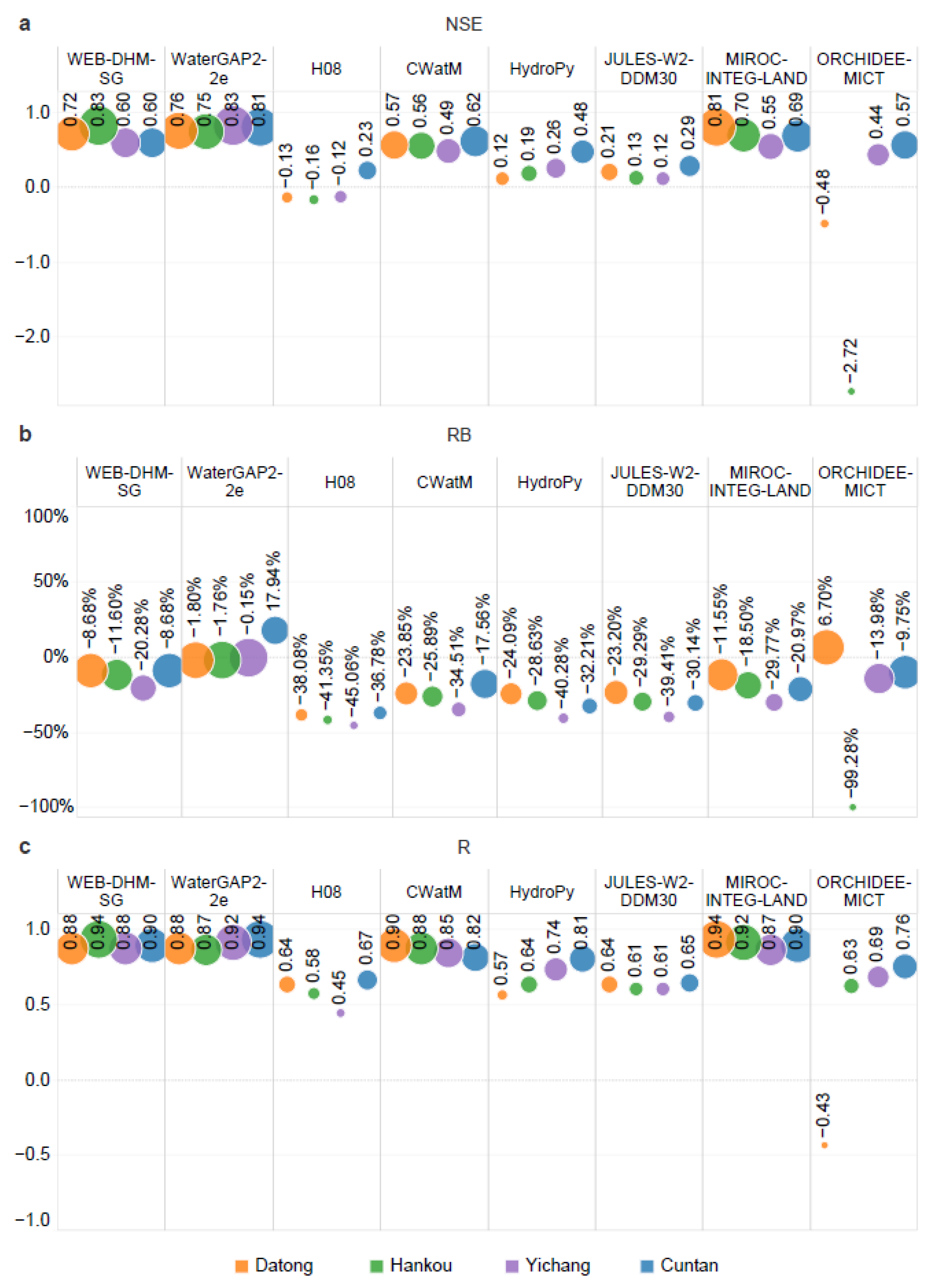
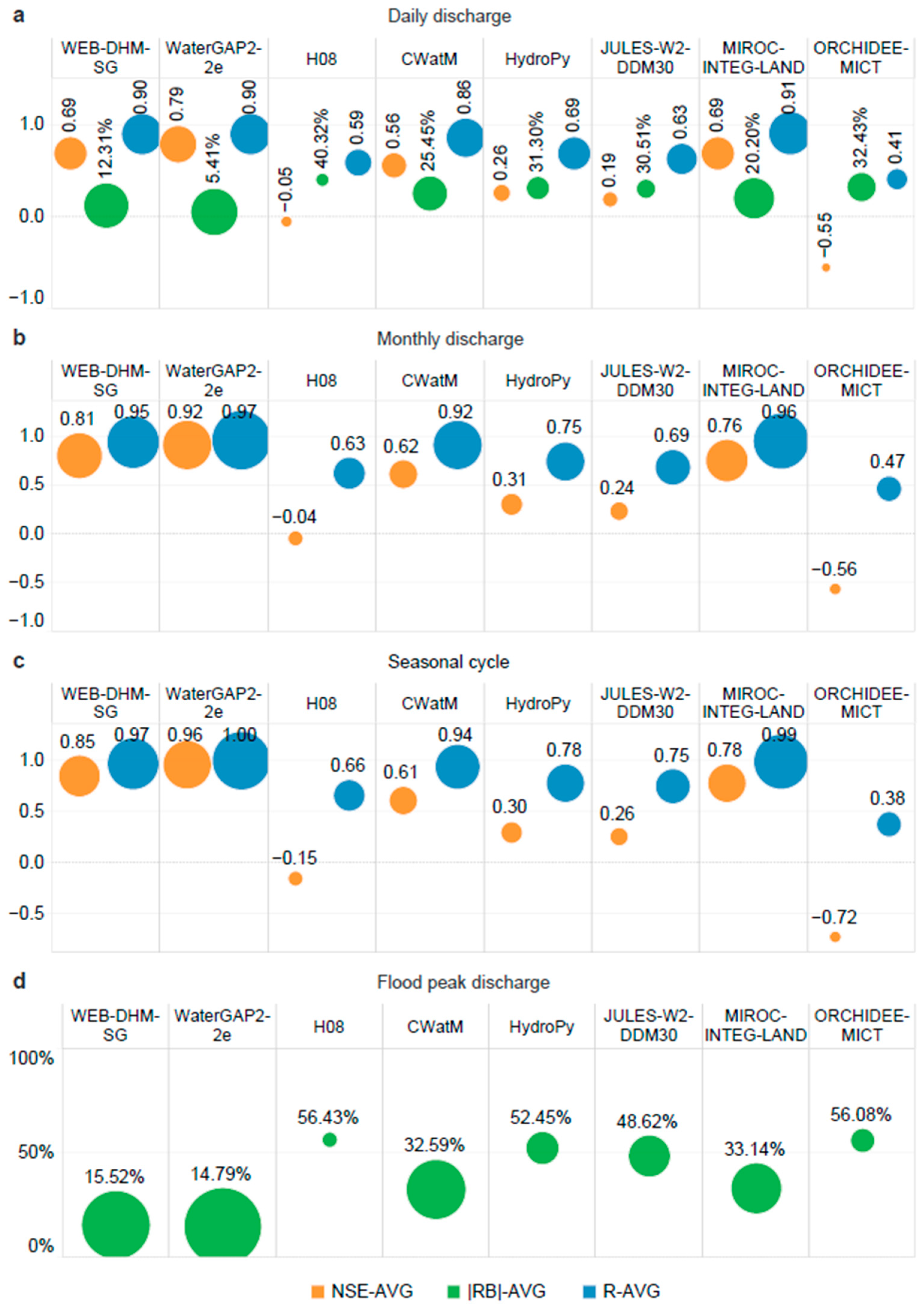
Daily scale performance based on NSE, RB, and R is summarized in Figure 2, while the corresponding observed and simulated discharge time series are provided in Figures S1–S4. Detailed gauge-level metrics are reported in Tables S2–S5, with cross-gauge averages in Table S6. Model performance differed substantially across the eight configurations.

Across the four gauges, the WaterGAP2-2e configuration achieved the highest station-averaged NSE (0.79) and the smallest mean absolute RB (5.41%), whereas MIROC-INTEG-LAND achieved the highest mean R (0.91) (Table S6). Among the remaining configurations, WEB-DHM-SG showed the most balanced daily scale performance across NSE, RB, and R, whereas H08 and ORCHIDEE-MICT showed the weakest daily scale skill. The most pronounced station-specific anomaly occurred for ORCHIDEE-MICT at Hankou, where NSE and RB reached −2.72 and −99.28%, respectively. A supplementary diagnostic check identified 9490 valid daily pairs and no missing, zero, or negative simulated values, indicating that the extreme metrics reflected a persistent discharge-magnitude mismatch rather than incomplete or invalid records (Table S22). Additional daily scale diagnostics are provided in the Taylor diagram (Figure S17) and the 1:1 plots (Figures S20–S23).

3.2. Monthly Changes

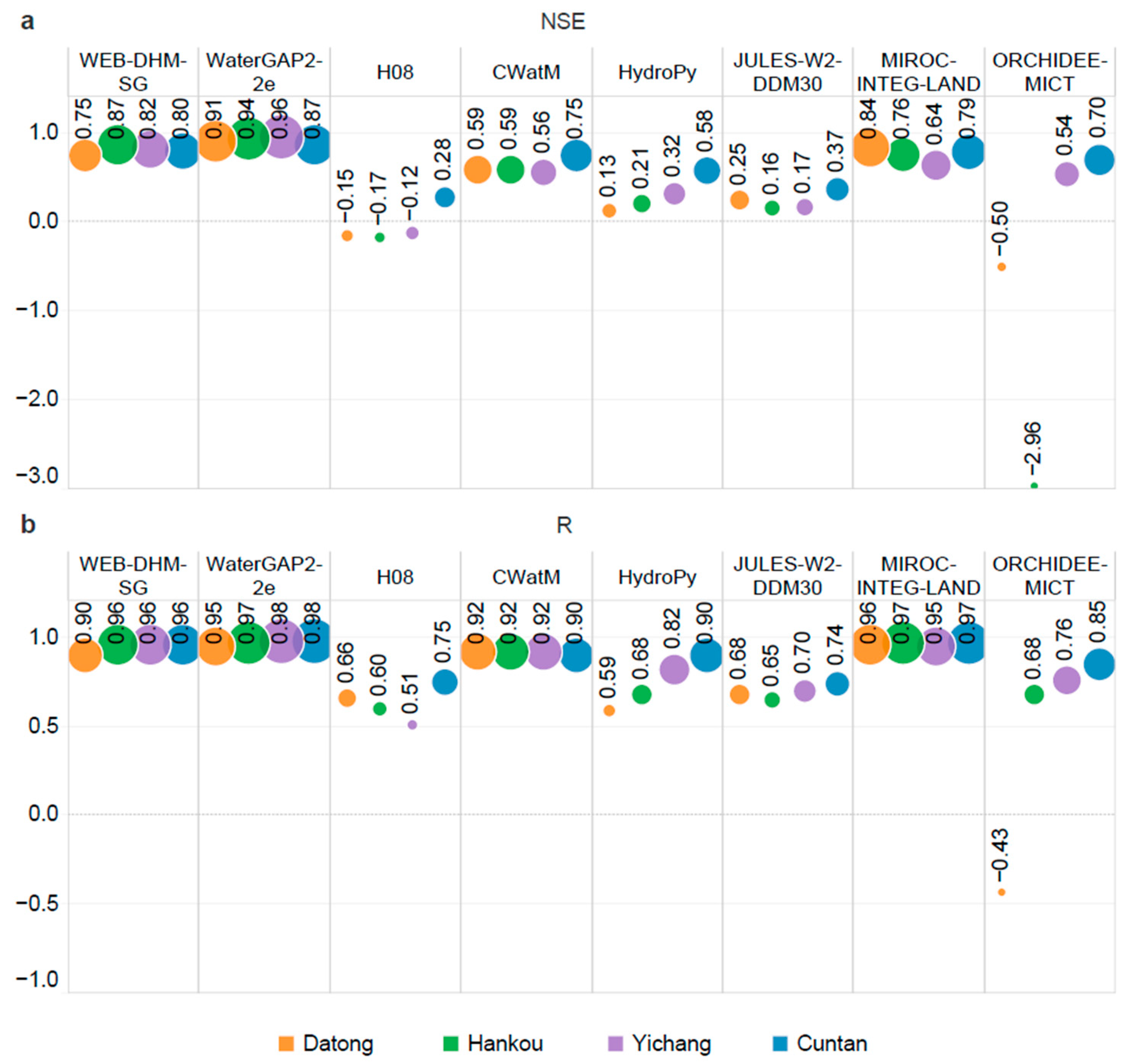
Monthly scale performance based on NSE and R is summarized in Figure 3, while the corresponding observed and simulated monthly discharge series are provided in Figures S5–S8. Detailed gauge-level metrics are reported in Tables S7–S10, with cross-gauge averages in Table S11.

Monthly scale performance was generally higher than daily scale performance. The WaterGAP2-2e configuration achieved the highest station-averaged NSE (0.92) and R (0.97) and produced the smallest monthly MAE at all four gauges (Table S11). WEB-DHM-SG and MIROC-INTEG-LAND also showed consistently high monthly scale skill, whereas H08 and ORCHIDEE-MICT had negative mean NSE values. ORCHIDEE-MICT remained particularly weak at Hankou, with NSE = −2.96 despite a moderate correlation, indicating a substantial error in simulated discharge magnitude. Additional monthly scale diagnostics are provided in the Taylor diagram (Figure S18) and the 1:1 plots (Figures S24–S27).

3.3. Seasonal Cycle

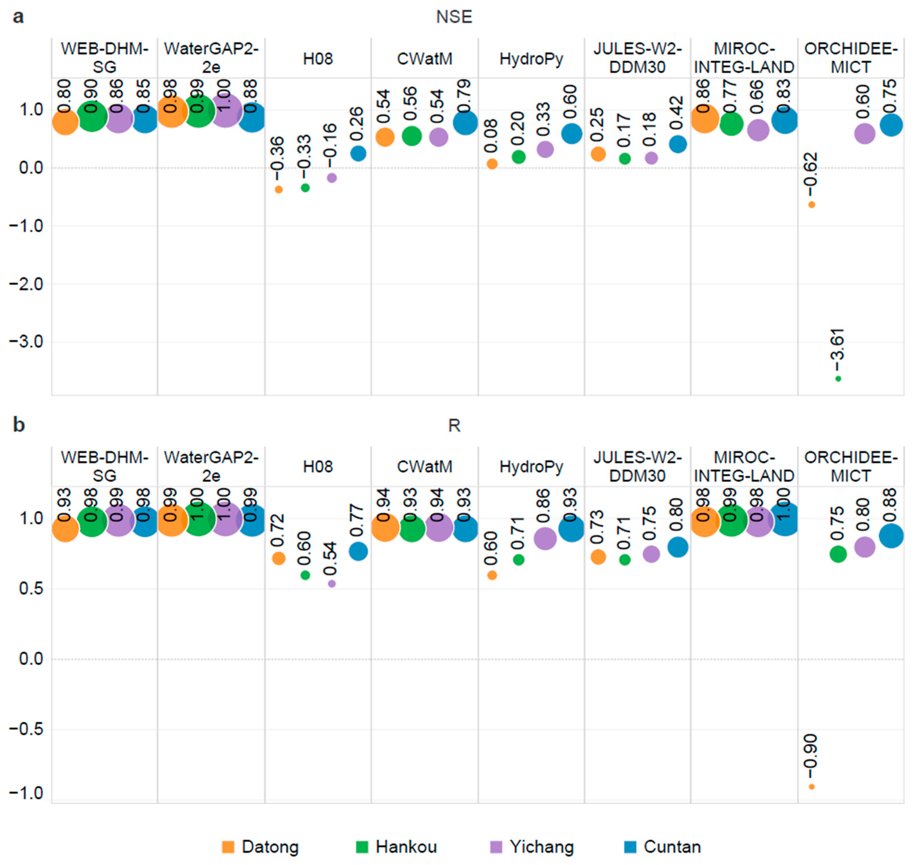
Seasonal-cycle performance based on NSE and R is summarized in Figure 4, while the corresponding observed and simulated seasonal cycles are provided in Figures S9–S12. Detailed gauge-level metrics are reported in Tables S12–S15, with cross-gauge averages in Table S16.

The WaterGAP2-2e configuration showed the strongest overall seasonal-cycle performance, with a station-averaged NSE of 0.96, R of 1.00, and the smallest MAE (Table S16). WEB-DHM-SG and MIROC-INTEG-LAND formed the next-best group, with mean NSE values of 0.85 and 0.78, respectively. In contrast, H08 and ORCHIDEE-MICT retained negative mean NSE values despite the additional temporal averaging. Together, the MAE results in Tables S12–S16 and the Taylor-diagram diagnostics in Figure S19 indicate that high correlation does not necessarily imply accurate seasonal amplitude, because some configurations with strong R values still showed comparatively large absolute errors, normalized-standard-deviation differences, or centered errors.

3.4. Flow-Percentile Performance

Flow-percentile diagnostics reveal that model skill varies substantially across different parts of the discharge distribution (Tables S18–S21). WaterGAP2-2e generally showed relatively small percentile biases at most stations. By contrast, WEB-DHM-SG, although showing high NSE and R at several gauges, exhibited large negative biases in the low-flow range. Its Q₀₅ bias reached −63.95% at Datong, −83.92% at Hankou, −95.69% at Yichang, and −96.78% at Cuntan, indicating a systematic underestimation of low-flow magnitudes. However, its high-flow percentile bias was much smaller at some stations, such as Q₉₅ = −4.15% at Datong, −6.42% at Hankou, and 5.75% at Yichang. Other models also showed distinct percentile-dependent behavior. H08, HydroPy, and JULES-W2-DDM30 generally underestimated middle- to high-flow percentiles, whereas ORCHIDEE-MICT showed highly station-dependent behavior. At Hankou, ORCHIDEE-MICT strongly underestimated all percentiles, with biases close to −99%, consistent with its weak daily and monthly performance at this station.

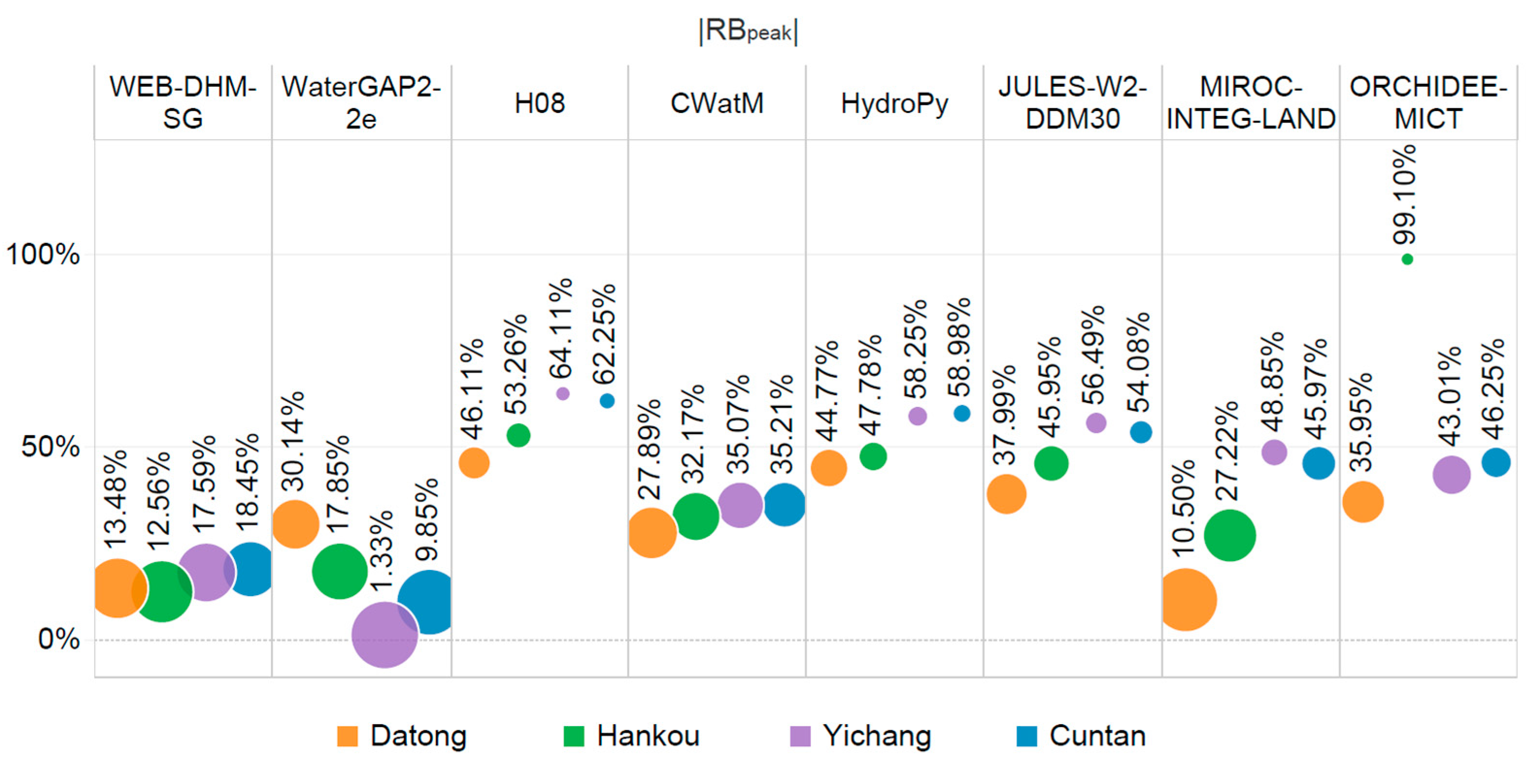
3.5. Annual Peak-Discharge Performance

Annual peak discharge was evaluated in terms of both temporal change and peak-flow magnitude bias. Figure 5 summarizes the station-level absolute peak-flow Relative Bias (|RB_peak|), whereas the corresponding annual peak-discharge series, OLS-fitted slopes, and Mann–Kendall significance results are provided in Figures S13–S16. The fitted slopes of the observed and simulated series were positive at Datong and Hankou and negative at Yichang and Cuntan. The Mann–Kendall tests indicated that the observed annual peak-discharge trends were not statistically significant at any of the four gauges (p > 0.05). For the simulated series, none of the trends were statistically significant at Datong or Hankou. WaterGAP2-2e and MIROC-INTEG-LAND produced statistically significant decreases at Yichang, whereas CWatM produced a statistically significant decrease at Cuntan. Slope direction and Mann–Kendall significance were therefore interpreted separately. Complete model-specific significance results are shown in Figures S13–S16.

Peak-flow magnitude performance also varied substantially across models and stations. Based on the station-averaged |RB_peak| (Figure 6d; Table S17), WaterGAP2-2e (14.79%) and WEB-DHM-SG (15.52%) formed the group with the smallest peak-flow biases. CWatM (32.59%) and MIROC-INTEG-LAND (33.14%) showed intermediate biases, whereas JULES-W2-DDM30, HydroPy, ORCHIDEE-MICT, and H08 all had station-averaged |RB_peak| values above 40%. Notable station-specific cases included the near-total underestimation of annual peak-discharge magnitude by ORCHIDEE-MICT at Hankou (RB_peak = −99.10%) and the overestimation by WaterGAP2-2e at Datong (RB_peak = 30.14%).

3.6. Common-Period Sensitivity Analysis

The supplementary 1976–2001 common-period analysis produced cross-model patterns broadly consistent with those obtained from the primary station-specific full-record evaluation (Tables S24–S27). WaterGAP2-2e remained the most consistently strong configuration across the daily, monthly, and seasonal-cycle summary metrics, with daily NSE changing from 0.79 to 0.81, while the monthly and seasonal-cycle NSE remained at 0.92 and 0.96, respectively. WEB-DHM-SG retained relatively strong NSE and bias-related performance, with mean |RB| changing from 12.31% to 12.10% and mean |RBpeak| from 15.52% to 14.21%. MIROC-INTEG-LAND continued to show high correlations across the three temporal scales, whereas H08 and ORCHIDEE-MICT retained comparatively weak NSE performance. The annual peak-discharge grouping also remained similar, with WaterGAP2-2e and WEB-DHM-SG showing the smallest mean |RBpeak| values. Although minor metric-specific changes in relative ordering occurred among closely performing models, restricting all gauges to 1976–2001 did not materially alter the principal cross-model patterns represented by the cross-gauge summary metrics.

4. Discussion

This study reveals marked performance differences among the eight ISIMIP3a GHMs. Across the descriptive station-averaged diagnostics shown in Figure 6, WaterGAP2-2e showed the most consistently strong performance among the evaluated standard ISIMIP3a configurations. Because the gauge-level metrics underlying this cross-gauge synthesis were calculated over different historical evaluation periods, Figure 6 should not be interpreted as a controlled common-period ranking. Nevertheless, the supplementary 1976–2001 common-period analysis reproduced the principal cross-model patterns represented by the cross-gauge summary metrics (Tables S24–S27), with only minor metric-specific changes in relative ordering. This indicates that the principal interpretation of Figure 6 is not solely an artifact of the unequal historical evaluation windows. This result must be interpreted in the context of its inherited global discharge calibration and other configuration features, including model structure, routing, and human–water representation, rather than as evidence of intrinsic structural superiority. Yichang, Hankou, and Datong coincide with gauges in the WaterGAP2-2e calibration-station dataset, whereas Cuntan does not; however, this spatial correspondence does not establish that the calibration and evaluation used identical observation periods or discharge records. The relatively strong performance at Cuntan provides evidence of performance beyond the identified calibration-gauge locations, but the present design cannot isolate calibration effects from other configuration differences. Accordingly, the following comparisons concern complete model configurations rather than isolated calibration, routing, or structural effects.

The higher metric-based performance at monthly and seasonal-cycle scales partly reflects the smoothing effect of temporal aggregation. Monthly discharge was calculated by averaging the daily series, and the seasonal cycle was further obtained by averaging the same calendar months across years. These successive averaging steps reduce the influence of short-term fluctuations and event-scale timing or magnitude errors, allowing the evaluation to emphasize the more persistent seasonal discharge pattern. In contrast, annual peak discharge was defined as the maximum daily discharge in each year and therefore retains event-scale errors rather than averaging them out. Peak-flow performance is consequently more sensitive to errors in the magnitude and timing of individual flood events and to uncertainties in meteorological forcing, particularly precipitation, as well as limitations in runoff-generation and routing processes.

Among the remaining configurations, WEB-DHM-SG showed the strongest overall performance in terms of NSE and bias-related diagnostics and had the smallest station-averaged absolute peak-flow bias (|RBpeak| = 15.52%). Its relatively strong performance is consistent with its explicit coupling of hydrological and hydrodynamic simulations [24,25,26], although the contribution of this routing representation cannot be isolated from other configuration differences in the present evaluation. However, this characterization applies primarily to general discharge dynamics and peak-flow magnitude rather than to all flow regimes. WEB-DHM-SG substantially underestimated Q05 at all four gauges, with biases reaching −95.69% at Yichang and −96.78% at Cuntan, indicating limited reliability for low-flow simulation. Although Q05 provides a low-flow diagnostic, dedicated drought and ecological-flow indicators were not evaluated in this study; therefore, such applications would require additional independent validation rather than being inferred from the overall NSE, R, or RB results.

In contrast, the H08 model systematically underestimated daily discharge at all four gauges (RB = −36.78% to −45.06%; Tables S2–S5) and showed weak daily scale performance, with negative NSE values at Datong, Hankou, and Yichang. These results indicate limited transferability of the standard H08 configuration to the Yangtze River Basin under the present evaluation framework. Given that H08 retained climate-zone-specific parameter optimization rather than Yangtze-specific discharge calibration [44], its weak performance may partly reflect limitations in transferring this parameterization to the basin; however, the present evaluation cannot isolate parameterization effects from other configuration differences.

The ORCHIDEE-MICT configuration showed strongly station-dependent performance, with an extreme discharge-magnitude underestimation at Hankou across daily, monthly, seasonal-cycle, flow-percentile, and annual peak-discharge diagnostics. The diagnostic check further showed that this anomaly was not attributable to missing or invalid records (Table S22). Because the daily biases at Datong, Yichang, and Cuntan were substantially smaller, the near-total discharge-magnitude underestimation appears specific to Hankou rather than reflecting a uniform basin-wide scaling bias. However, the available diagnostics confirm the magnitude anomaly but do not identify its cause. Possible runoff-generation, routing, grid-cell matching, or other configuration issues therefore require further investigation, and the Hankou result should be interpreted cautiously. At the monthly scale, CWatM performed better at Cuntan (NSE = 0.75) than at the three downstream gauges (NSE = 0.56–0.59; Tables S7–S10). This spatial contrast may be associated with station-dependent differences in hydrological regulation, routing, contributing-area representation, water use, or other configuration factors; however, their individual contributions cannot be isolated in the present evaluation.

These contrasting behaviors indicate that model suitability is application-dependent rather than represented by a single overall ranking. Models that reproduce general discharge dynamics well may still perform poorly for low flows or flood peaks. Model selection should therefore consider the target temporal scale and flow regime, particularly whether the application emphasizes overall discharge dynamics, low-flow conditions, or flood-peak simulation.

These findings are broadly consistent with, but also extend, previous GHM evaluations. The strong performance of the evaluated WaterGAP2-2e configuration is consistent with broader evidence that parameter estimation and calibration can improve GHM performance [11,20]. In the present study, however, models representing human–water processes did not perform uniformly better than those without such representations, indicating that human–water process representation is only one component of regional model skill. This finding complements recent global evidence that discharge performance can deteriorate as human impacts intensify and that challenges remain in representing human activities in heavily managed regions [8].

In contrast to the general tendency toward global discharge overestimation reported by Heinicke et al. [12], the Yangtze results include both positive and negative biases, indicating substantial regional and model dependence. The pronounced station-dependent performance of several models further supports the need for basin-scale evaluation and cautious assessment of regional model transferability [10]. The difficulty in reproducing annual peak discharge is also consistent with previous GHM flood-evaluation and multi-model flood-assessment studies [13,14]. The flood-related findings should therefore be interpreted as diagnostics of high-flow magnitude and annual-peak behavior rather than as a comprehensive evaluation of flood-event dynamics. Because peak timing, exceedance frequency, flood volume, and flood duration were outside the evaluation scope, the results should not be interpreted as a complete assessment of flood hazards. Future evaluations could also incorporate complementary temporal diagnostics beyond monotonic trends, as recent ISIMIP-based studies have demonstrated the value of examining changes in the temporal regularity and dominant periods of climate-impact extremes under global warming [54].

This study has several limitations. First, the evaluation was based on four major mainstem gauges and therefore primarily constrains integrated mainstem discharge responses rather than tributary, headwater, high-elevation, or reservoir-regulated sub-basin processes. The selected model grid cells were identified using gauge coordinates and mainstem alignment, but their upstream contributing areas were not quantitatively matched to the reported gauge drainage areas, and no lag optimization applied. Residual grid-to-gauge, contributing-area, and travel-time mismatches may therefore affect the station-based metrics. Second, the primary station-specific evaluation periods differ because longer continuous in situ records were unavailable for all gauges. The primary station-averaged metrics therefore combine different historical windows and should still be interpreted as descriptive cross-gauge summaries rather than strictly controlled common-period rankings. However, the supplementary 1976–2001 analysis produced broadly consistent cross-model summary patterns, indicating that the principal Figure 6 conclusions are relatively robust to this difference in evaluation windows, despite minor metric-specific changes in relative ordering.

Third, the WaterGAP2-2e evaluation was not fully independent of calibration because three of the four evaluation gauges overlapped with its calibration dataset. Reservoir regulation also remains an unresolved source of inter-model uncertainty because reservoir processes differ among the standard ISIMIP3a configurations and the available downstream observations do not support a consistent before-and-after assessment of Three Gorges regulation. In addition, uncertainty in the GSWP3-W5E5 forcing was not independently evaluated, and none of the models were recalibrated specifically for the Yangtze River Basin. Because no process-isolation experiments were performed, the individual effects of calibration, parameterization, routing, reservoir representation, and other human–water processes cannot be quantified separately. Accordingly, the reported rankings should be interpreted as comparisons of complete standard model configurations rather than as controlled comparisons of intrinsic model structures or the performance achievable after basin-specific calibration.

Despite these limitations, this study provides more than an overall ranking of the eight GHMs. Relative to previous Yangtze studies that have mainly focused on the regional calibration and application of individual models [20], the present analysis establishes a mainstem gauge-based benchmark of standard ISIMIP3a configurations across temporal scales and flow regimes. By integrating daily, monthly, seasonal-cycle, flow-percentile, and annual peak-discharge diagnostics, the study shows that model suitability is scale- and flow-regime dependent and that apparent superiority must be interpreted in the context of inherited calibration and configuration. Identifying these performance trade-offs and regime-specific weaknesses constitutes the main contribution of the study.

5. Conclusions

The evaluation of eight standard ISIMIP3a GHM configurations at four principal Yangtze mainstem gauges revealed strong dependence of model performance on temporal scale and flow regime. Metric-based performance generally increased from daily to monthly and seasonal-cycle scales, consistent with the smoothing of short-term timing and magnitude errors through temporal aggregation, whereas annual peak discharge remained more difficult to reproduce. WaterGAP2-2e showed the most consistently strong performance across these temporal-scale evaluations, although this result should be interpreted in light of its inherited global discharge calibration and other configuration differences.

For the other evaluated configurations, WEB-DHM-SG showed the strongest overall performance in terms of NSE and bias-related diagnostics and had the smallest station-averaged absolute peak-flow bias (|RB_peak| = 15.52%), although MIROC-INTEG-LAND showed slightly higher station-averaged correlations across the daily, monthly, and seasonal-cycle evaluations. In contrast, H08 and ORCHIDEE-MICT showed the weakest overall performance, with negative NSE values and large peak-flow biases.

Overall, no single configuration performed uniformly well across temporal scales and flow regimes. The supplementary 1976–2001 common-period analysis yielded broadly consistent cross-gauge summary patterns, indicating that the principal Figure 6 results were robust to the unequal gauge-specific evaluation windows. The results therefore provide a cross-diagnostic benchmark for application-specific model selection and targeted model improvement in regional discharge simulation and peak-flow-related applications. Several limitations should be noted explicitly: the evaluation was restricted to four Yangtze mainstem gauges and therefore provides limited coverage of tributary, headwater, high-elevation, and reservoir-regulated sub-basin processes; the primary cross-gauge summaries combine gauge-specific records from different historical periods; the common GSWP3-W5E5 forcing dataset was not independently evaluated; and no model was recalibrated specifically for the Yangtze River Basin. Accordingly, the apparent model rankings should be interpreted as diagnostics of the evaluated standard ISIMIP3a configurations rather than as a controlled comparison of intrinsic model structures or as the upper bound of performance achievable after basin-specific calibration.

References

1. Sood, A.; Smakhtin, V. Global hydrological models: A review. Hydrol. Sci. J. 2015, 60, 549–565. [Google Scholar] [CrossRef] [Scilit]
2. Bierkens, M.F.P. Global hydrology 2015: State, trends, and directions. Water Resour. Res. 2015, 51, 4923–4947. [Google Scholar] [CrossRef] [Scilit]
3. Mandel, A.; Battiston, S.; Monasterolo, I. Mapping global financial risks under climate change. Nat. Clim. Change 2025, 15, 329–334. [Google Scholar] [CrossRef] [Scilit]
4. Grant, L.; Vanderkelen, I.; Gudmundsson, L.; Fischer, E.; Seneviratne, S.I.; Thiery, W. Global emergence of unprecedented lifetime exposure to climate extremes. Nature 2025, 641, 374–379. [Google Scholar] [CrossRef] [Scilit] [PubMed]
5. Gosling, S.N.; Schmied, H.M.; Bradley, A.; Burek, P.; Chang, J.; Ciais, P.; Grillakis, M.; Guillaumot, L.; Hanasaki, N.; Hartley, A.; et al. ISIMIP3a Simulation Data from the Global Water Sector (v1.5); ISIMIP Repository: Potsdam, Germany, 2025. [Google Scholar] [CrossRef]
6. Rosenzweig, C.; Arnell, N.W.; Ebi, K.L.; Lotze-Campen, H.; Raes, F.; Rapley, C.; Smith, M.S.; Cramer, W.; Frieler, K.; Reyer, C.P.O.; et al. Assessing inter-sectoral climate change risks: The role of ISIMIP. Environ. Res. Lett. 2017, 12, 010301. [Google Scholar] [CrossRef] [Scilit]
7. Lange, S.; Mengel, M.; Treu, S.; Büchner, M. ISIMIP3a Atmospheric Climate Input Data (v1.2); ISIMIP Repository: Potsdam, Germany, 2022. [Google Scholar] [CrossRef]
8. Tiwari, A.D.; Pokhrel, Y.; Boulange, J.; Burek, P.; Guillaumot, L.; Gosling, S.N.; Grillakis, M.; Hanasaki, N.; Koutroulis, A.; Ostberg, S.; et al. Similarities and divergent patterns in hydrologic fluxes and storages simulated by global water models. Nat. Water 2025, 3, 550–560. [Google Scholar] [CrossRef] [Scilit]
9. Veldkamp, T.I.E.; Zhao, F.; Ward, P.J.; de Moel, H.; Aerts, J.C.J.H.; Schmied, H.M.; Portmann, F.T.; Masaki, Y.; Pokhrel, Y.; Liu, X.; et al. Human impact parameterizations in global hydrological models improve estimates of monthly discharges and hydrological extremes: A multi-model validation study. Environ. Res. Lett. 2018, 13, 055008. [Google Scholar] [CrossRef] [Scilit]
10. Siderius, C.; Biemans, H.; Kashaigili, J.J.; Conway, D. Going local: Evaluating and regionalizing a global hydrological model’s simulation of river flows in a medium-sized East African basin. J. Hydrol. Reg. Stud. 2018, 19, 349–364. [Google Scholar] [CrossRef] [Scilit]
11. Kupzig, J.; Reinecke, R.; Pianosi, F.; Flörke, M.; Wagener, T. Towards parameter estimation in global hydrological models. Environ. Res. Lett. 2023, 18, 074023. [Google Scholar] [CrossRef] [Scilit]
12. Heinicke, S.; Volkholz, J.; Schewe, J.; Gosling, S.N.; Müller Schmied, H.; Zimmermann, S.; Mengel, M.; Sauer, I.J.; Burek, P.; Chang, J.; et al. Global hydrological models continue to overestimate river discharge. Environ. Res. Lett. 2024, 19, 074005. [Google Scholar] [CrossRef] [Scilit]
13. Yang, T.; Sun, F.; Gentine, P.; Liu, W.; Wang, H.; Yin, J.; Du, M.; Liu, C. Evaluation and machine learning improvement of global hydrological model-based flood simulations. Environ. Res. Lett. 2019, 14, 114027. [Google Scholar] [CrossRef] [Scilit]
14. Huang, S.; Kumar, R.; Rakovec, O.; Aich, V.; Wang, X.; Samaniego, L.; Liersch, S.; Krysanova, V. Multimodel assessment of flood characteristics in four large river basins at global warming of 1.5, 2.0 and 3.0 K above the pre-industrial level. Environ. Res. Lett. 2018, 13, 124005. [Google Scholar] [CrossRef] [Scilit]
15. Ye, X.; Zhang, Z.; Xu, C.-Y.; Liu, J. Attribution Analysis on Regional Differentiation of Water Resources Variation in the Yangtze River Basin under the Context of Global Warming. Water 2020, 12, 1809. [Google Scholar] [CrossRef] [Scilit]
16. Su, Z.; Ho, M.; Hao, Z.; Lall, U.; Sun, X.; Chen, X.; Yan, L. The impact of the Three Gorges Dam on summer streamflow in the Yangtze River Basin. Hydrol. Processes 2020, 34, 705–717. [Google Scholar] [CrossRef] [Scilit]
17. Zhou, R. Economic growth, energy consumption and CO2 emissions—An empirical study based on the Yangtze River economic belt of China. Heliyon 2023, 9, e19865. [Google Scholar] [CrossRef] [Scilit] [PubMed]
18. Birkinshaw, S.J.; Guerreiro, S.B.; Nicholson, A.; Liang, Q.; Quinn, P.; Zhang, L.; He, B.; Yin, J.; Fowler, H.J. Climate change impacts on Yangtze River discharge at the Three Gorges Dam. Hydrol. Earth Syst. Sci. 2017, 21, 1911–1927. [Google Scholar] [CrossRef] [Scilit]
19. Gao, S.; Ti, C.-P.; Tang, S.-R.; Wang, X.-L.; Wang, H.-Y.; Meng, L.; Yan, X.-Y. Runoff Simulation and Its Response to Extreme Precipitation in the Yangtze River Basin. Environ. Sci. 2023, 44, 4853–4862. [Google Scholar] [CrossRef] [Scilit] [PubMed]
20. Zhao, F.; Nie, N.; Liu, Y.; Yi, C.; Guillaumot, L.; Wada, Y.; Burek, P.; Smilovic, M.; Frieler, K.; Buechner, M.; et al. Benefits of Calibrating a Global Hydrological Model for Regional Analyses of Flood and Drought Projections: A Case Study of the Yangtze River Basin. Water Resour. Res. 2025, 61, e2024WR037153. [Google Scholar] [CrossRef] [Scilit]
21. Chen, J. Hydrological Characteristics of the Yangtze River. In Evolution and Water Resources Utilization of the Yangtze River; Chen, J., Ed.; Springer: Singapore, 2020; pp. 123–162. [Google Scholar]
22. Yang, S.L.; Milliman, J.D.; Xu, K.H.; Deng, B.; Zhang, X.Y.; Luo, X.X. Downstream sedimentary and geomorphic impacts of the Three Gorges Dam on the Yangtze River. Earth-Sci. Rev. 2014, 138, 469–486. [Google Scholar] [CrossRef] [Scilit]
23. Cheng, G.; Liu, Y.; Chen, Y.; Gao, W. Spatiotemporal variation and hotspots of climate change in the Yangtze River Watershed during 1958–2017. J. Geogr. Sci. 2022, 32, 141–155. [Google Scholar] [CrossRef] [Scilit]
24. Qi, W.; Feng, L.; Yang, H.; Liu, J. Warming winter, drying spring and shifting hydrological regimes in Northeast China under climate change. J. Hydrol. 2022, 606, 127390. [Google Scholar] [CrossRef] [Scilit]
25. ISIMIP. Impact Model: WEB-DHM-SG. Available online: https://www.isimip.org/impactmodels/details/208/?query=WEB-DHM-SG#tab_isimip3a (accessed on 20 October 2025).
26. Yamazaki, D.; Kanae, S.; Kim, H.; Oki, T. A physically based description of floodplain inundation dynamics in a global river routing model. Water Resour. Res. 2011, 47, W04501. [Google Scholar] [CrossRef] [Scilit]
27. Müller Schmied, H.; Trautmann, T.; Ackermann, S.; Cáceres, D.; Flörke, M.; Gerdener, H.; Kynast, E.; Peiris, T.A.; Schiebener, L.; Schumacher, M.; et al. The global water resources and use model WaterGAP v2.2e: Description and evaluation of modifications and new features. Geosci. Model Dev. 2024, 17, 8817–8852. [Google Scholar] [CrossRef] [Scilit]
28. Hanasaki, N.; Yoshikawa, S.; Pokhrel, Y.; Kanae, S. A global hydrological simulation to specify the sources of water used by humans. Hydrol. Earth Syst. Sci. 2018, 22, 789–817. [Google Scholar] [CrossRef] [Scilit]
29. Burek, P.; Satoh, Y.; Kahil, T.; Tang, T.; Greve, P.; Smilovic, M.; Guillaumot, L.; Zhao, F.; Wada, Y. Development of the Community Water Model (CWatM v1.04)—A high-resolution hydrological model for global and regional assessment of integrated water resources management. Geosci. Model Dev. 2020, 13, 3267–3298. [Google Scholar] [CrossRef] [Scilit]
30. ISIMIP. Impact Model: CWatM. Available online: https://www.isimip.org/impactmodels/details/257/?query=CWatM#tab_isimip3a (accessed on 20 October 2025).
31. Stacke, T.; Hagemann, S. HydroPy (v1.0): A new global hydrology model written in Python. Geosci. Model Dev. 2021, 14, 7795–7816. [Google Scholar] [CrossRef] [Scilit]
32. Best, M.J.; Pryor, M.; Clark, D.B.; Rooney, G.G.; Essery, R.L.H.; Ménard, C.B.; Edwards, J.M.; Hendry, M.A.; Porson, A.; Gedney, N.; et al. The Joint UK Land Environment Simulator (JULES), model description—Part 1: Energy and water fluxes. Geosci. Model Dev. 2011, 4, 677–699. [Google Scholar] [CrossRef] [Scilit]
33. ISIMIP. Impact Model: JULES-W2-DDM30. Available online: https://www.isimip.org/impactmodels/details/358/?query=JULES-W2-DDM30 (accessed on 20 October 2025).
34. Clark, D.B.; Mercado, L.M.; Sitch, S.; Jones, C.D.; Gedney, N.; Best, M.J.; Pryor, M.; Rooney, G.G.; Essery, R.L.H.; Blyth, E.; et al. The Joint UK Land Environment Simulator (JULES), model description—Part 2: Carbon fluxes and vegetation dynamics. Geosci. Model Dev. 2011, 4, 701–722. [Google Scholar] [CrossRef] [Scilit]
35. Yokohata, T.; Kinoshita, T.; Sakurai, G.; Pokhrel, Y.; Ito, A.; Okada, M.; Satoh, Y.; Kato, E.; Nitta, T.; Fujimori, S.; et al. MIROC-INTEG-LAND version 1: A global biogeochemical land surface model with human water management, crop growth, and land-use change. Geosci. Model Dev. 2020, 13, 4713–4747. [Google Scholar] [CrossRef] [Scilit]
36. Guimberteau, M.; Zhu, D.; Maignan, F.; Huang, Y.; Yue, C.; Dantec-Nédélec, S.; Ottlé, C.; Jornet-Puig, A.; Bastos, A.; Laurent, P.; et al. ORCHIDEE-MICT (v8.4.1), a land surface model for the high latitudes: Model description and validation. Geosci. Model Dev. 2018, 11, 121–163. [Google Scholar] [CrossRef] [Scilit]
37. ISIMIP. Impact Model: ORCHIDEE-MICT. Available online: https://www.isimip.org/impactmodels/details/361/?query=The%20ORCHIDEE-MICT (accessed on 20 October 2025).
38. ISIMIP. Impact Model: WaterGAP2-2e. Available online: https://www.isimip.org/impactmodels/details/313/?query=WaterGAP2-2e#tab_isimip3a (accessed on 20 October 2025).
39. ISIMIP. Impact Model: H08. Available online: https://www.isimip.org/impactmodels/details/52/?query=H08#tab_isimip3a (accessed on 20 October 2025).
40. ISIMIP. Impact Model: HydroPy. Available online: https://www.isimip.org/impactmodels/details/287/?query=HydroPy (accessed on 20 October 2025).
41. ISIMIP. Impact Model: MIROC-INTEG-LAND. Available online: https://www.isimip.org/impactmodels/details/333/?query=MIROC-INTEG-LAND#tab_isimip3a (accessed on 20 October 2025).
42. ISIMIP. Global Impact Model Database. Available online: https://www.isimip.org/ (accessed on 20 October 2025).
43. Müller Schmied, H.; Cáceres, D.; Eisner, S.; Flörke, M.; Herbert, C.; Niemann, C.; Peiris, T.A.; Popat, E.; Portmann, F.T.; Reinecke, R.; et al. The global water resources and use model WaterGAP v2.2d: Model description and evaluation. Geosci. Model Dev. 2021, 14, 1037–1079. [Google Scholar] [CrossRef] [Scilit]
44. Yoshida, T.; Hanasaki, N.; Nishina, K.; Boulange, J.; Okada, M.; Troch, P.A. Inference of Parameters for a Global Hydrological Model: Identifiability and Predictive Uncertainties of Climate-Based Parameters. Water Resour. Res. 2022, 58, e2021WR030660. [Google Scholar] [CrossRef] [Scilit]
45. Döll, P.; Lehner, B. Validation of a new global 30-min drainage direction map. J. Hydrol. 2002, 258, 214–231. [Google Scholar] [CrossRef] [Scilit]
46. Schewe, J.; Schmied, H.M. DDM30 River Routing Network for ISIMIP3; ISIMIP Repository: Potsdam, Germany, 2022. [Google Scholar] [CrossRef]
47. Cáceres, D.; Marzeion, B.; Malles, J.H.; Gutknecht, B.D.; Müller Schmied, H.; Döll, P. Assessing global water mass transfers from continents to oceans over the period 1948–2016. Hydrol. Earth Syst. Sci. 2020, 24, 4831–4851. [Google Scholar] [CrossRef] [Scilit]
48. Nash, J.E.; Sutcliffe, J.V. River flow forecasting through conceptual models part I—A discussion of principles. J. Hydrol. 1970, 10, 282–290. [Google Scholar] [CrossRef] [Scilit]
49. Pearson, K. Note on Regression and Inheritance in the Case of Two Parents. Proc. R. Soc. Lond. 1895, 58, 240–242. [Google Scholar] [CrossRef] [Scilit]
50. Willmott, C.J.; Matsuura, K. Advantages of the mean absolute error (MAE) over the root mean square error (RMSE) in assessing average model performance. Clim. Res. 2005, 30, 79–82. [Google Scholar] [CrossRef] [Scilit]
51. Taylor, K.E. Summarizing multiple aspects of model performance in a single diagram. J. Geophys. Res. Atmos. 2001, 106, 7183–7192. [Google Scholar] [CrossRef] [Scilit]
52. Gupta, H.V.; Kling, H.; Yilmaz, K.K.; Martinez, G.F. Decomposition of the mean squared error and NSE performance criteria: Implications for improving hydrological modelling. J. Hydrol. 2009, 377, 80–91. [Google Scholar] [CrossRef] [Scilit]
53. Mann, H.B. Nonparametric Tests Against Trend. Econometrica 1945, 13, 245–259. [Google Scholar] [CrossRef] [Scilit]
54. Zantout, K.; Balkovic, J.; Billing, M.; Folberth, C.; Gosling, S.N.; Hank, T.; Hantson, S.; Iizumi, T.; Ito, A.; Jägermeyr, J.; et al. Shifting dominant periods in extreme climate impacts under global warming. Nat. Commun. 2025, 16, 9746. [Google Scholar] [CrossRef] [Scilit] [PubMed]
Figure 1. Location of the Yangtze River Basin and the flow-gauging stations used in this study. Red dots indicate the hydrological stations, black open squares indicate the corresponding 0.5° grid cells, blue lines indicate the river network, and cyan triangles mark three representative large reservoirs, namely Xiluodu, Xiangjiaba, and the Three Gorges Reservoir, along the upper and middle Yangtze mainstem. These reservoirs are shown to provide geographic context relative to the evaluation gauges and do not constitute a complete inventory of reservoirs in the basin. Their display does not imply identical reservoir representation across the eight GHMs.
Water 18 02076 g001
Figure 2. Summary of daily scale discharge simulation performance for the eight global hydrological models at the four gauging stations. (a) Nash–Sutcliffe Efficiency (NSE), (b) Relative Bias (RB, %), (c) Pearson’s correlation coefficient (R). Colored bubbles represent Datong, Hankou, Yichang, and Cuntan, and the numerical labels indicate the corresponding metric values. Bubble size indicates metric-based performance: larger bubbles correspond to higher NSE and R values, whereas for RB, they correspond to smaller |RB| values. The complete observed and simulated daily discharge time series are provided in Figures S1–S4.
Water 18 02076 g002
Figure 3. Summary of monthly scale discharge simulation performance for the eight global hydrological models at the four gauging stations. (a) Nash–Sutcliffe Efficiency (NSE); (b) Pearson’s correlation coefficient (R). Colored bubbles represent Datong, Hankou, Yichang, and Cuntan, and the numerical labels indicate the corresponding metric values. Larger bubbles correspond to higher NSE and R values, indicating better metric-based performance. The complete observed and simulated monthly discharge series are provided in Figures S5–S8.
Water 18 02076 g003
Figure 4. Summary of seasonal-cycle discharge simulation performance for the eight global hydrological models at the four gauging stations. (a) Nash–Sutcliffe Efficiency (NSE); (b) Pearson’s correlation coefficient (R). Colored bubbles represent Datong, Hankou, Yichang, and Cuntan, and the numerical labels indicate the corresponding metric values. Larger bubbles correspond to higher NSE and R values, indicating better metric-based performance. The complete observed and simulated seasonal cycles are provided in Figures S9–S12.
Water 18 02076 g004
Figure 5. Absolute peak-flow Relative Bias (|RBpeak|) of the eight global hydrological models at Datong, Hankou, Yichang, and Cuntan. Models are shown on the horizontal axis; colors distinguish the four gauges, and numerical labels indicate the corresponding |RBpeak| values. Lower |RBpeak| indicates smaller peak-flow bias; accordingly, larger bubbles correspond to smaller |RBpeak| values. The corresponding annual peak-discharge time series and trend analyses are shown in Figures S13–S16.
Water 18 02076 g005
Figure 6. Comparison of discharge-simulation performance among global hydrological models based on cross-gauge mean metrics. (a) Daily scale results. (b) Monthly scale results. (c) Seasonal-cycle results. (d) Annual peak-discharge results. NSE = Nash–Sutcliffe Efficiency. R = Pearson’s correlation coefficient. RB = Relative Bias of the discharge series; RBpeak = Relative Bias of annual peak-discharge magnitude. The horizontal axis shows the models, and the vertical axis shows the metric values. AVG denotes the unweighted arithmetic mean of the corresponding gauge-level values across the four gauges, with each gauge-level value calculated over its station-specific evaluation period. For bias-based metrics, absolute gauge-level values were averaged to avoid cancelation between positive and negative biases. AVG provides a descriptive cross-gauge summary and does not represent either a ranking based on a common historical period or an area-weighted basin-wide hydrological average. Bubble size indicates metric-based performance: larger bubbles correspond to higher NSE and R values, whereas for bias-based metrics they correspond to smaller absolute biases. In panel (a), the cross-gauge bias summary is mean |RB|, whereas in panel (d), it is mean |RBpeak|. A supplementary sensitivity analysis in which all four gauges were evaluated over the common period 1976–2001 is provided in Tables S24–S27.
Water 18 02076 g006