A Framework for Evaluating Meteorological Drought Indices as Indicators of Low Flows: A Case Study of the Biała Lądecka River Catchment Area

Abstract

Meteorological, soil, and hydrological droughts are among the most important phenomena affecting the natural environment and water management. Prolonged precipitation deficits often result in low river flows, reducing water resources and degrading aquatic ecosystems. This study evaluates the potential of meteorological drought indices as predictors of observed low flows. Long-term meteorological and hydrological data, including precipitation and river discharge records, were analyzed for the Biała Lądecka River catchment in Lower Silesia, southwestern Poland. Meteorological drought was characterized using the Standardized Precipitation Index (SPI) and the Standardized Precipitation Evapotranspiration Index (SPEI) calculated for 1-, 3-, and 6-month timescales, together with corresponding one- and two-week indices. Relationships between drought index values and observed low flows were analyzed while accounting for the time lag of the catchment response. The predictive performance of individual indices was evaluated to determine their suitability for water resource monitoring and management. The results show that meteorological drought indices can effectively indicate the occurrence of low flows, although the strength of the relationships depends on the adopted timescale. Both classical and short-term indices proved useful for analyzing the development of hydrological drought and have potential applications in low-flow monitoring and early warning systems.

1. Introduction

Drought is a common phenomenon, yet it lacks a single definition [1]. Depending on the context, one can distinguish meteorological, soil, or hydrological droughts—each of these, although interrelated, may have slightly different causes and consequences. Meteorological and soil droughts pose the greatest threat to crops and plant production. Hydrological drought also affects water supply, degradation of aquatic ecosystems, and deterioration of water quality. Meteorological, soil, hydrological, and combined drought indicators were described and compiled by [2].

Due to Poland’s geographical configuration, virtually all available water comes from precipitation occurring exclusively over its territory. Therefore, with a slight simplification, it can be assumed that the water flowing through rivers is the remainder of what fell with precipitation and did not evaporate. When periods of low rainfall and meteorological conditions favoring intense evaporation are observed, water shortages in the environment arise, which in the literature are referred to as periods of drought and meteorological drought. These are occurring increasingly frequently and have a significant impact, among other things, on water levels in watercourses [3]. In recent years, low or very low water levels have been frequently observed, even in Poland’s largest rivers. In July and August 2025, record low water levels were observed in the Vistula River—according to a water meter, they even fell below 20 cm. On 22 August 2025, the water level in Warsaw fell below 11 cm—the previous historical minimum [4].

Since meteorological data used to determine classic meteorological drought indices are relatively readily available, the question arises: can these indices serve as predictors of observed low flows? The aim of this study was to present a methodological framework for assessing the potential of meteorological drought indices to indicate observed low flows, illustrated using a section of the Biała Lądecka River basin in the Kłodzko Land as a case study. The case study provides an initial demonstration of the applicability of the proposed framework; however, further validation using additional catchments and independent datasets is required before its broader predictive capability can be assessed.

1.1. Meteorological Drought and Meteorological Drought Markers

Meteorological drought is defined as a period with a precipitation deficit relative to the long-term average conditions for a given location or area [5]. Two classic meteorological drought indices are identified: the Standardized Precipitation Index (SPI) [6] and the Standardized Precipitation Evaporation Index (SPEI) [7]. Both compare the studied period with similar multi-year periods, allowing for the determination of the extent to which a given period differs from the long-term average. The SPI and SPEI show the deviations of observed precipitation totals in a selected period relative to a multi-year reference period for the same accumulation range [5]. The literature distinguishes classic temporal approaches to the SPI and SPEI (monthly and multi-month), which, calculated for different accumulation periods, indicate different potential effects of meteorological drought [5]. The obtained index values are numerically similar—a summary of possible values and the resulting classification are shown in

Table 1. Classification of the analyzed period depending on the SPI/SPEI value.

Class of the Analyzed Period	SPI/SPEI Index Value Range
Extremely dry	SPI $\le -2$
Very dry	$-2<$ SPI $\le -1.5$
Dry	$-1.5<$ SPI $\le -1$
Normal	$-1<$ SPI $\le 1$
Wet	$1<$ SPI $\le 1.5$
Very wet	$1.5<$ SPI $\le 2$
Extremely wet	$2<$ SPI

. The Python package spei, version 0.8.2, was used to calculate the values of meteorological drought indices [8].

1.2. SPI Index

The SPI is calculated based on precipitation totals over a given multi-year period, by fitting a gamma distribution to this precipitation data series, followed by standardization. Therefore, an a priori assumption about the gamma distribution of the data must be made. However, [9] indicates that this distribution fits precipitation data series well. The procedure for determining the SPI value was implemented based on [10].

1.3. SPEI Index

The SPEI [7,11] includes evapotranspiration in addition to daily precipitation totals for the analyzed period. This means that it is not, like the SPI, an indicator solely measuring precipitation deficits, but rather accounts for increased water demand resulting from high temperatures. It can therefore be used to monitor agricultural and hydrological droughts in a warming climate [12].

The SPEI is calculated based on the climatic water balance $D=P-PET$, where P is the total precipitation and $PET$ is the potential evaporation. Ref. [7] demonstrated that the distribution of the random variable D does not conform to a normal distribution, and their results suggested choosing a log-logistic distribution to standardize the D series.

The simplest approach to calculating $PET$ was proposed by [13], which based the index solely on the mean monthly temperature. This approach was used in the original work on the construction of the SPEI [7]. However, other methods of calculating $PET$ are also used to determine the SPEI [14]. Another method for calculating $PET$, then usually denoted by $E{T}_0$ and called reference evaporation, recommended by FAO-56, is the Penman–Monteith (PM) method [15]. This method provides the most accurate results, but is also difficult to apply due to its dependence on many variables (temperature, wind speed, radiation intensity, air humidity parameters). The PM method was abandoned in this study due to insufficient measurement data. However, having at hand the mean, minimum and maximum daily temperatures, it was decided to use the Hargreaves–Samani (HS) method [16], which, like the Thornthwaite method [13], is used as an approximation and simplification of $PET$ estimation.

Studies [17,18,19] indicate that the appropriately calibrated [20] HS method provides the best approximation of $E{T}_0$ calculated using the PM method among temperature-based models. Appropriate calibration of parameters in the HS method is necessary due to the diversity of climatic conditions across the globe. For the purposes of this publication, the following HS method parameters were adopted, determined after [21] as optimal for the climatic conditions prevailing in Poland:

$$E{T}_0=0.408·R_a(T_a+17.8){(T_{max}-T_{min})}^{0.724},$$

(1)

where $R_a$—radiation intensity at the boundary of the atmosphere on a horizontal surface, expressed by the formula

$$R_a={\displaystyle \frac{24·60}{\pi }}{G}_{sc}{d}_r({\delta }_{s}sin\left(\varphi \right)sin\left(\delta \right)+cos\left(\varphi \right)cos\left(\delta \right)sin\left({\omega }_s\right)),$$

(2)

where $G_{s}c$—solar constant ($0.0820$ MJ· m⁻² ·min⁻¹); $d_r$—relative Earth–Sun distance; ${\omega }_s$—sunset angle; $\varphi$—latitude (in radians); and $\delta$—solar declination.

1.4. Drought Propagation

There are four main types of drought: meteorological, soil (agricultural), hydrological and hydrogeological [22,23,24]. The former means a periodic shortage or low rainfall; in the latter, water begins to be scarce in the soil, particularly for plants. The next stage, to simplify, is water shortage in watercourses, meaning restrictions in surface and underground runoff. Hydrogeological drought is a decrease in water content, even in the deeper layers of the Earth’s surface. It is important to remember that a temporary improvement in meteorological conditions may alleviate soil drought, but it will not reduce hydrological or hydrogeological drought. Only a long-term change in weather—many months of increased rainfall—can alleviate hydrological and hydrogeological drought. Due to drought propagation, many studies analyze the SPI and SPEI in relation to the Standardized Streamflow Index (SSI) [25,26,27,28] and the Standardized Runoff Index (SRI) [29,30,31,32]. Ref. [33] speaks directly about the potential of the SPI and SPEI to predict droughts related to water flow. The relationship between successive phases of drought propagation is undeniable, and its strength and timing depend on many factors, both climatic and environmental [34]. This paper focuses solely on one aspect of the relationship between meteorological drought and hydrological drought, attempting to assess the lag time with which low flows can be observed as a consequence of precipitation deficit.

1.5. Low Flows

Hydrological drought is associated with periodically low flows in rivers and depletion of reservoir reserves [1]. The proper determination of the limiting flow value, below which a low flow can be considered, depends on the nature of the stream, climatic conditions, and hydrological regime. Economic criteria are also important. There are methods for determining limiting flow based on the highest flow value from annual minimums [35], low-flow deficit volume [36], or settling curves [37].

The limiting discharge for low flow for permanent rivers ranges between characteristic flow values Q70 and Q90 [1,22]. The characteristic flow QX is determined for a given measuring station based on the flow-duration curve as the flow value occurring or exceeded for X% of the time. Ref. [1] assumes Q70 as the limiting discharge. For comparison, the authors of this paper assumed limiting discharges at levels Q70, Q80, and Q90. However, the mere fact that a flow occurred below a fixed level was significant in the analyses. The number of consecutive days with low flow or the volume of the low-flow deficit was not taken into account [36]. As a consequence of the adopted assumptions, the authors will not discuss the phenomenon of low flow, but rather the events of the low flows, because the mere event of a flow below a fixed level does not meet the definition of a low flow.

2. Materials and Methods

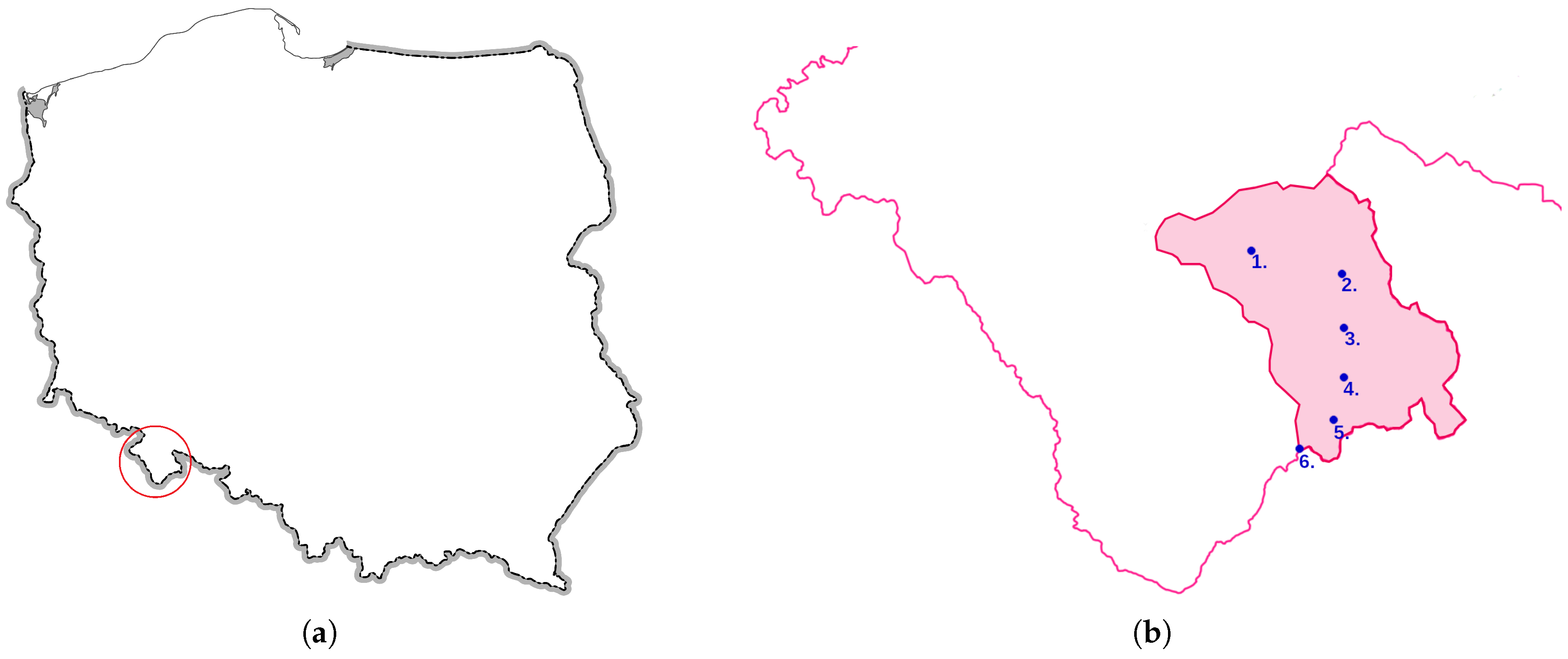
Testing the adopted methods was limited to a fragment of the Kłodzko Land, which includes the Biała Lądecka River catchment area (Figure 1). The first approach used meteorological data from the synoptic station in Kłodzko and the hydrological station in Kłodzko on the Nysa Kłodzka River. The second approach relied on data from six meteorological stations (Ołdrzychowice Kłodzkie, Lądek Zdrój, Stronie Śląskie, Bolesławów, Kamienica, Śnieżnik) and the hydrological station in Żelazno. The data came from IMGW-PIB measurement and observation stations. Due to the limited availability of temperature measurements for the study area, data from ref. [38] were also used. All analyzed data came from the 2011–2024 multiannual period.

Measurements from meteorological stations included daily temperatures (average, minimum, and maximum) and daily precipitation. Measurements from hydrological stations related to daily flow volume (Q) were used.

2.1. Empirical Short-Term Drought Index Based on SPI and SPEI Methodology

According to ref. [5], the standard timescales for the SPI and SPEI indices are 1-, 3-, and 6-month periods, and longer periods, covering 12, 24, and 48 months. The SPI/SPEI-1 reflect short-term rainfall deficits and can be used, among other things, to assess reduced flows in small streams. The SPI/SPEI-3 and SPI/SPEI-6 indices describe seasonal drought conditions and are useful in assessing changes in water resources and the occurrence of reduced flows.

This study focuses on monthly accumulation periods. Three-month indices were also calculated for periods corresponding to the seasons spring (April–June) and summer (July–September), as well as six-month indices for the growing season (April–September), which is crucial for the functioning of ecosystems and water management. Longer timescales were omitted because they do not reflect the relatively rapid response of small mountain catchments to precipitation deficits.

However, in the case of the analyzed mountain catchment, the monthly timescale may be too long to capture rapid changes in hydrological conditions caused by precipitation deficits. Therefore, we proposed extending the classical methodology by using shorter aggregation periods for precipitation and climatic surplus data and constructing corresponding indices.

For this purpose, aggregation was used, which involves summing precipitation and climatic surplus values in time windows corresponding to one-week and two-week timescales. A one-week period was chosen as the shortest interval allowing for the identification of rapidly developing meteorological deficits, while a two-week period represents a compromise between rapid change detection and greater index stability. It allows for the reduction in the impact of random fluctuations observed in individual weeks while maintaining high temporal resolution.

The short-term indices were constructed based on the concepts of the SPI and SPEI. In classical indices, the estimation of distribution parameters is based on long monthly data series, for which the number of observations is sufficient to provide a stable fit. Due to the limited length of the time series, it was not possible to assume that the data conformed to the gamma distribution (used in the standard SPI) or the log-logistic distribution (used in the standard SPEI), which prevented the use of the classical parametric approach. Therefore, an empirical cumulative distribution function was used, which does not require a predetermined functional form and allows for consistent standardization even for very short timescales. The obtained values were then transformed to the standard normal distribution according to the procedure used in classical indices. As a result, the basic concept of the SPI and SPEI, which involves standardizing cumulative values to a normal distribution, was retained, only changing the method of estimating the cumulative distribution function.

Due to the use of an empirical cumulative distribution function instead of a classical parametric approach, the proposed indices are not direct equivalents of the classical SPI and SPEI. They should be interpreted as short-term drought indices inspired by the original SPI/SPEI methodology. They retain the basic concept of these indices, which involves transforming cumulative values of precipitation or climatic surplus to a standardized normal scale, enabling comparison of deficit intensity over time. The modification concerns the method of estimating the cumulative distribution function, which was necessary due to the limitations of very short timescales and the instability of parametric distribution fitting.

It should also be emphasized that the classical SPI and SPEI indices were developed for monthly and longer timescales, so their direct interpretation for one- or two-week periods would be limited. With such short aggregation, the obtained values may reflect short-term precipitation variability more than the cumulative moisture deficit characteristic of meteorological drought. For this reason, the proposed indices should be treated as standardized short-term anomalies, analogous to the classic SPI and SPEI, enabling the identification of short-term episodes of meteorological deficit, and not as their direct equivalents. To simplify descriptions, short-term indices inspired by the SPI and SPEI methodology are referred to in this paper as short-term SPI/SPEI-like indices.

2.2. Meteorological Drought Indices, Point and Spatial

The SPI and SPEI (one, three, and six months), as well as their short-term equivalents (one and two weeks), were calculated using two different approaches: point-based and spatial.

The point-based approach relied on measurements from adjacent stations: one hydrological and one meteorological. Due to the availability of temperature measurements necessary to estimate $E{T}_0$, measurement data from the synoptic station in Kłodzko and hydrological measurements from the Kłodzko station on the Nysa Kłodzka River were used.

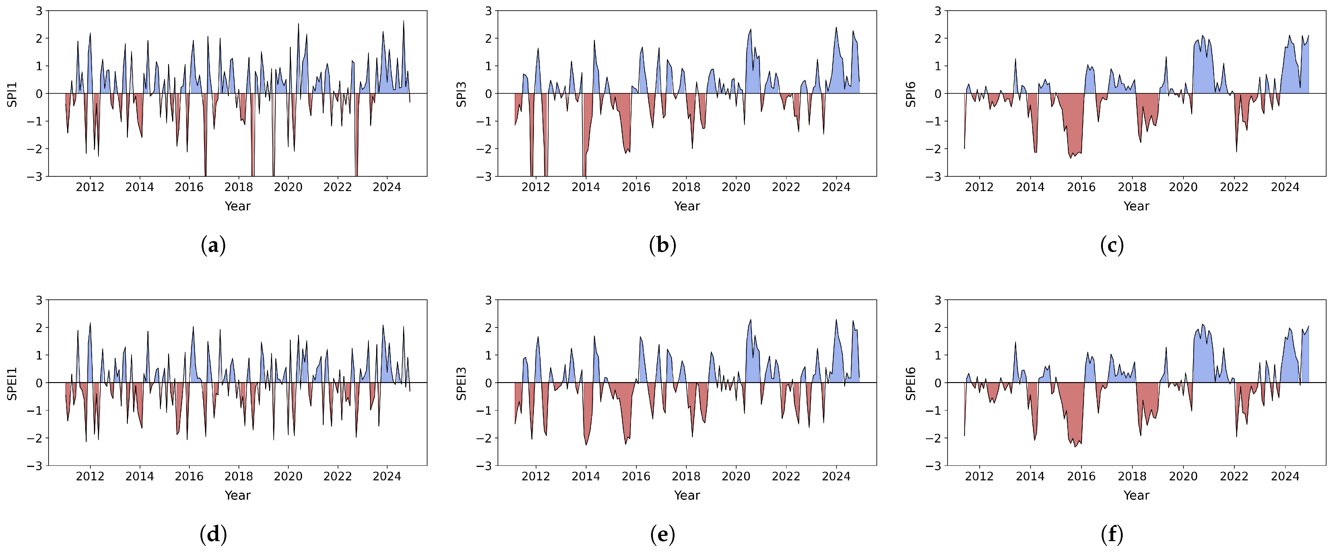
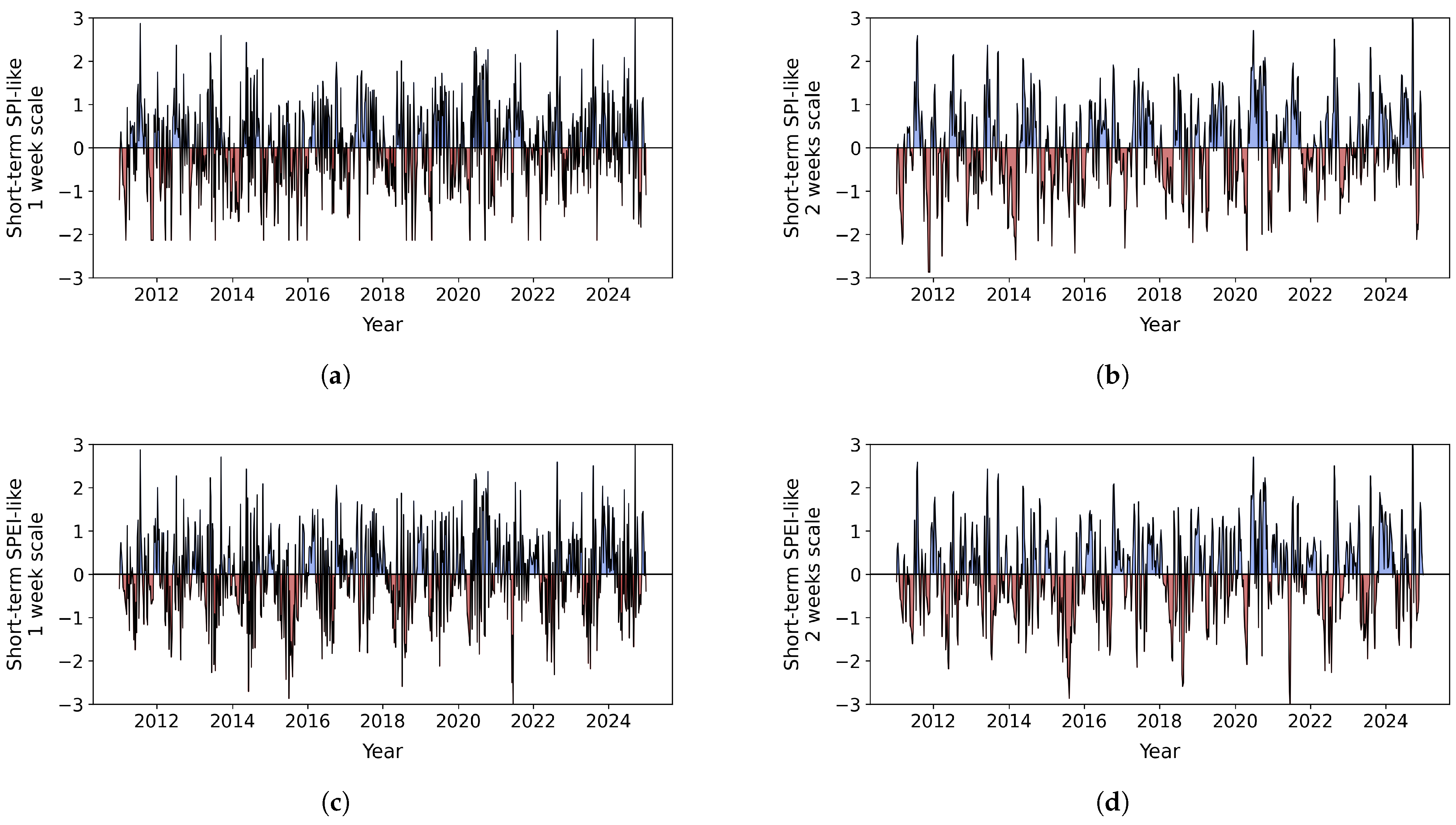
The spatial approach aimed to calculate indices reflecting average meteorological conditions within the Biała Lądecka River basin, enclosed by the Żelazno hydrological station. Average daily precipitation was calculated based on data from all precipitation stations within the basin. Due to the unavailability of temperature measurement data, it was decided to use data from the ERA5-Land dataset [38]. Data were collected from six nodal points located within the basin, and the average daily temperature was calculated. The combined values of the one-, three-, and six-month SPI and SPEI, as well as their one- and two-week equivalents, are presented in Figure 2 and Figure 3.

Regardless of the approach, series of SPI/SPEI or short-term SPI/SPEI-like indices were obtained for the analyzed time intervals. According to the interpretation of the indices, binary series were created by assigning a value of 1 when the index value was −1 or less and 0 when the index value was higher than −1. Therefore, series were obtained indicating the occurrence of a drought episode, regardless of its severity. The consequence of the binary classification of SPI/SPEI and short-term SPI/SPEI-like indices is the loss of information regarding the intensity of meteorological drought. However, this approach was implemented intentionally, as the goal of the analysis was to identify periods of drought episodes and assess their relationship with low flows, rather than to assess the intensity of drought in individual periods. According to the concept of meteorological drought propagation into hydrological drought, it can be assumed that the occurrence of a rainfall deficit may be reflected in subsequent episodes of low flows or contribute to their increased intensity. The use of binary classification allows for the assessment of the ability of meteorological indices to identify periods of potential risk of hydrological low flows.

2.3. Low Flows in the Studied Area

Data from hydrological stations included daily flow measurements, so to make the SPI/SPEI series comparable with the hydrological data, they had to be scaled to the same resolution. Data regarding the SPI/SPEI and their short-term counterparts, both before and after the creation of binary series, were considered on a 1-, 3-, or 6-month scale, and a 1- or 2-week scale. Daily flows had to be aggregated into analogous binary series. The following criterion was adopted: if a given month had at least eight days of low flow, the month was considered a low-flow month. If a given week had at least two days of low flow, the week was considered a low-flow week. It should be noted that flow aggregation was performed only for weekly and monthly series. Subsequent comparisons of the resulting binary series were performed in the following scheme: 1 week SPI/SPEI—the same week of flows, 2 weeks SPI/SPEI—the second of these weeks of flows and, for example, 3 months SPI/SPEI—the last of these months of flows.

The first approach utilized data from the hydrological station in Kłodzko. Readings from this station depend on the flows of the three main rivers of the Kłodzko Land (Nysa Kłodzka, Biała Lądecka, and Bystrzyca Dusznicka) and their tributaries. The station aggregates information from almost the entire Kłodzko Land.

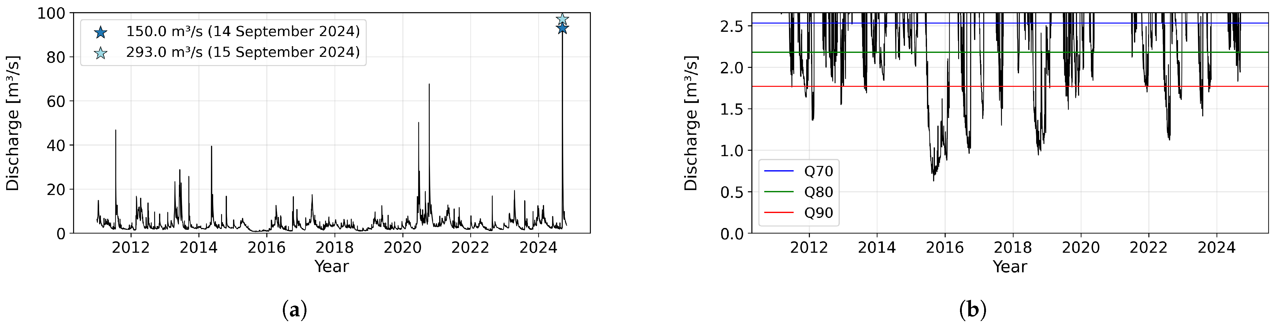
Under the spatial approach, aimed at linking meteorological drought with low flows, the study area was limited to the Biała Lądecka River basin, enclosing it with the hydrological station in Żelazno, which used data from this main river (and its tributaries). Daily flows from the 2011–2024 period and their relationship to watershed levels are presented in Figure 4.

For the flow series, the approach described above was analogous to that used for meteorological data. Based on the adopted flow criteria of Q70, Q80, and Q90, binary series were created for each individual stream, with 1 indicating a week or month with flows below the established threshold, and 0 indicating the opposite. Also in this case, the information derived from the data was intentionally reduced to information about the occurrence or absence of low flow. This approach allowed for the treatment of hydrological low flows as binary events, allowing for a direct comparison of their occurrence with meteorological drought episodes and the application of statistical methods based on the analysis of qualitative variables. However, it should be emphasized that this simplification does not take into account the severity of the low flow or its duration, so the results should be interpreted as an assessment of the relationship between the occurrence of events, not as an analysis of the quantitative relationship between meteorological deficit and flow rate.

2.4. Binary Series

Binary series relating to the occurrence of a drought episode were compared with series relating to the occurrence of low-flow episodes (Figure 5 and Figure 6).

For each pair of binary series, drought and flow, the relationship between the hydrological variable and the meteorological variable was analyzed. It was analyzed whether the response of the binary low-flow index would be immediate, meaning a positive drought index in the selected time period would result in a positive low-flow index at the same time, or whether the response occurred with a delay (lag). Series of SPI/SPEI and their short-term counterparts were prepared, taking into account their time shift in the flow index response, ranging from 0 to 4 (months or weeks, depending on whether weekly or monthly indices were considered). To examine the dependence between pairs of series, a contingency table was created for each pair of binary series, based on which the Pearson independence test statistics ${\chi }^2$ without Yates’ correction were calculated. The following assumptions were made:

H₀: 

The occurrence of a drought episode and a low flow are independent events.

H₁: 

The events are not independent.

The test statistic is expressed by the formula

$${\chi }^2=\sum _{i,j}{\displaystyle \frac{{(O_{ij}-E_{ij})}^2}{E_{ij}}},$$

(3)

where $O_{ij}$—observed events; $E_{ij}$—expected events. The dimension of the array determines the shape of the ${\chi }^2$ distribution through degrees of freedom ($df$),

$$df=(r-1)(c-1),$$

(4)

where r is the number of rows and c is the number of columns. For each cell in the table, the expected value is calculated as follows:

$$E_{ij}={\displaystyle \frac{n_i·n_j}{N}},$$

(5)

where $n_i$ is the sum of the ith row, $n_j$ is the sum of the jth column, and N is the number of observations in the sample.

An example calculation of the ${\chi }^2$ test statistic and the p-value is provided in Appendix A.

The strength of the relationship was assessed using Cramér’s V coefficient:

$$V=\sqrt{{\displaystyle \frac{{\chi }^2}{N}}},$$

(6)

where N is the number of observations in the sample.

For a 2 × 2 contingency table, Cramér’s V coefficient is identical to the $\varphi$ coefficient.

The optimal offset was assumed to be the lag corresponding to the maximum value of Cramér’s V coefficient. The corresponding p-value of the ${\chi }^2$ test was also recorded.

The offset was intended to indicate the time after the drought episode that low flow could be expected. The analyses also addressed the following questions:

• What is the probability of low flows occurring after a meteorological drought? ($P(Q=1|M=1)$);
• What is the probability of a meteorological drought occurring during a low-flow event? ($P(M=1|Q=1)$).

The answers to these questions were analyzed both before and after the meteorological data were shifted. The results are summarized in tables in the individual subsections.

The ability of meteorological indices to detect the occurrence of low flows was assessed using the conditional probability value $P(Q=1|M=1)$, while the overall classification ability to distinguish between the occurrence and absence of low flows was assessed using the True Skill Statistic ($TSS$) index metric [39,40], a measure of the quality of binary classification determined from the confusion matrix. The construction of $TSS$, following [41,42], is presented in

Table 2. Two-dimensional error matrix with component construction $TSS$. $TP$—true positive; $TN$—true negative; $FP$—false positive; $FN$—false negative.

		Validation Dataset
		Presence	Absence
Model	Presence	$TP$	$FP$
	Absence	$FN$	$TN$
		$Sensivity={\displaystyle \frac{TP}{\phantom{(}TP+FN}}$	$Specifity={\displaystyle \frac{TN}{\phantom{(}TN+FP}}$
		$TSS=Sensivity+Specifity-1$

. $TSS$ is one of the measures frequently used in hydrology, meteorology, and extreme event analysis [43,44,45]. Contingency tables are often used as a tool for evaluating discrete event forecasts [46].

An example of calculating the distance between two binary strings using the $TSS$ metric is presented in Appendix B.

The $ch{i}^2$ test therefore assesses the existence of a statistical relationship between the analyzed binary variables, but does not provide information on the strength of this relationship or the classification efficiency of the predictor. Therefore, the analysis was supplemented with the Cramér’s V coefficient, which determines the strength of the relationship between variables, and the $TSS$ metric, which assesses the quality of the classification based on a contingency table. In the analyzed approach, the contingency table provides the basis for assessing the ability of meteorological drought indices to indicate the occurrence of low flows. The $ch{i}^2$ test indicates whether the observed relationship is statistically significant, Cramér’s V determines its strength, and $TSS$ describes the classification efficiency of events.

Due to the binary nature of the analyzed time series, classical methods based on contingency tables were used, enabling a direct assessment of the relationship between the occurrence of meteorological drought and low flows. Alternatives to this approach would include, among others, the use of a contingency table. Logistic regression models or machine learning methods would enable the construction of predictive models and the estimation of the probability of an event taking into account additional explanatory variables. In this study, however, the goal was to determine the statistical dependence, the strength of the association, and the efficiency of event classification based on existing observations.

3. Results

The results presented below only concern spatial analyses for the Biała Lądecka River basin, enclosed by the Żelazno station. Conclusions should not be drawn based on the results indicating the relationship between meteorological precipitation and low water levels obtained from only one measurement point, as a rainfall deficit at just one point in the basin may not be reflected in low water levels. Given this observation, the focus was on spatial analyses.

3.1. Classical Approach (SPI and SPEI-1, 3, and 6) for the Catchment Area

The results for the monthly SPI and SPEI are summarized in

Table 3. Optimal offsets for pointer pairs Q–SPI/SPEI.

Boundary Flow	Meteorological Index	Optimum Lag (Monthly Scale)	$\mathit{P}(\mathit{Q}=1|\mathit{M}=1)$	$\mathit{P}(\mathit{M}=1|\mathit{Q}=1)$	TSS	${\mathit{\chi }}^2$	V Cramér’s V	p-Value
Q70	SPI-1	1	0.68	0.2	0.21	3.685	0.149	0.055
Q70	SPEI-1	1	0.72	0.21	0.26	5.538	0.182	0.018
Q70	SPI-3	0	0.81	0.2	0.35	9.197	0.234	0.002
Q70	SPEI-3	0	0.76	0.26	0.31	9.377	0.236	0.002
Q70	SPI-6	1	0.83	0.24	0.39	12.234	0.271	0.0004
Q70	SPEI-6	1	0.78	0.25	0.33	9.727	0.241	0.0018
Q80	SPI-1	1	0.56	0.24	0.25	5.867	0.187	0.015
Q80	SPEI-1	1	0.56	0.24	0.25	5.867	0.187	0.015
Q80	SPI-3	0	0.76	0.28	0.48	18.433	0.331	1.76 $\times {10}^{-5}$
Q80	SPEI-3	0	0.69	0.34	0.42	18.393	0.331	1.8 $\times {10}^{-5}$
Q80	SPI-6	0	0.75	0.31	0.47	20.293	0.348	6.643 $\times {10}^{-5}$
Q80	SPEI-6	0	0.7	0.33	0.43	18.287	0.33	1.9 $\times {10}^{-5}$
Q90	SPI-1	2	0.32	0.31	0.19	5.947	0.189	0.0147
Q90	SPEI-1	0	0.24	0.23	0.1	1.631	0.099	0.2
Q90	SPI-3	0	0.52	0.42	0.42	24.988	0.386	5.768 $\times {10}^{-7}$
Q90	SPEI-3	0	0.38	0.42	0.27	13.51	0.284	0.0002
Q90	SPI-6	0	0.54	0.5	0.45	32.04	0.437	1.508 $\times {10}^{-8}$
Q90	SPEI-6	1	0.52	0.54	0.43	32.255	0.439	1.352 $\times {10}^{-8}$

. For each Q–SPI/SPEI pair, the result with the highest $TSS$ value or the lowest p-value (the highest ${\chi }^2$ value) is presented. In most cases, the Q–SPI/SPEI pairs show an optimal fit without the need for a time shift. In six pairs of binary strings, applying a small (one or two month) lag improved the quality of the fit. With an increasing timescale of the index (from 1 to 6 months), an increase in the $TSS$ value and a decrease in the p-value was observed.

The best fit was obtained for the 3- and 6-month indices, particularly for the more restrictive thresholds (Q80 and Q90). In these cases, the values of $TSS$ reach the highest levels, and the relationships are statistically significant.

For two pairs (Q70–SPI-1 and Q90–SPEI-1), the distributions are not consistent both before and after the shift.

High values of the conditional probabilities $P(Q=1|M=1)$ with moderate values of $P(M=1|Q=1)$ indicate the asymmetric predictive ability of the model. Therefore, the indices can be used as a forecasting tool and to identify conditions favorable to low flows, but they do not explain all the causes of low flows. The values of $P(M=1|Q=1)$ increase with increasing restrictiveness of the threshold. This can be interpreted as a higher ability to explain hydrological phenomena by meteorological phenomena in the case of very low flows.

3.2. Short-Term SPI/SPEI-like Indices for the Catchment Area

The results for the weekly indices are summarized in

Table 4. Optimal offsets for pointer pairs Q–SPI/SPEI-like. The labels 1w and 2w denote one- and two-week timescales, respectively.

Boundary Flow	Meteorological Index	Optimum Lag (Monthly Scale)	$\mathit{P}(\mathit{Q}=1|\mathit{M}=1)$	$\mathit{P}(\mathit{M}=1|\mathit{Q}=1)$	TSS	${\mathit{\chi }}^2$	V Cramér’s V	p-Value
Q70	SPI-1w	1	0.57	0.2	0.14	7.893	0.104	0.005
Q70	SPEI-1w	3	0.62	0.22	0.2	15.19	0.144	9.706 $\times {10}^{-5}$
Q70	SPI-2w	1	0.63	0.22	0.2	16.27	0.149	5.493 $\times {10}^{-5}$
Q70	SPEI-2w	2	0.62	0.22	0.2	15.3	0.145	9.135 $\times {10}^{-5}$
Q80	SPI-1w	3	0.42	0.21	0.13	7.579	0.102	0.006
Q80	SPEI-1w	3	0.46	0.23	0.17	13.62	0.137	0.0002
Q80	SPI-2w	2	0.48	0.24	0.2	17.83	0.156	2.413 $\times {10}^{-5}$
Q80	SPEI-2w	3	0.46	0.23	0.17	13.62	0.137	0.0002
Q90	SPI-1w	3	0.25	0.24	0.1	7.851	0.104	0.005
Q90	SPEI-1w	4	0.29	0.3	0.16	18.94	0.161	1.346 $\times {10}^{-5}$
Q90	SPI-2w	3	0.28	0.28	0.14	14.92	0.143	0.0001
Q90	SPEI-2w	3	0.28	0.29	0.15	16.676	0.151	4.434 $\times {10}^{-5}$

. Unlike the monthly approach, in this case, the runoff response was delayed in all analyzed situations; the time shift improved the fit between the sequences. The best results were obtained for a lag of 1 to 4 weeks. In each case, the TSS values were higher after accounting for the shift, and the correlations remained or became statistically significant.

The SPEI-like indices demonstrate comparable or slightly higher performance than the SPI-like indices, indicating a significant role of evapotranspiration in shaping the analyzed phenomenon.

In the analysis based on weekly indices, TSS values generally remain lower than for monthly indices. The chi-square test statistic values also indicate weaker agreement between meteorological drought and low flows on short timescales.

The best correlations were obtained for 2-week indices, with a delayed runoff response of 1 to 3 weeks. In these cases, TSS values reach moderate levels, and the correlations are statistically significant, especially for the more restrictive threshold flows (Q80 and Q90).

The probability values of $P(Q=1|M=1)$ are lower than in the monthly analysis and rarely exceed the levels observed for monthly timescales, indicating the limited ability of weekly indices to predict low flows. At the same time, the values of $P(M=1|Q=1)$ remain relatively low, although they tend to increase with increasing restrictiveness of the limiting flow threshold.

The obtained results confirm the asymmetric nature of the relationship, although it is less pronounced than in the case of monthly timescales. Therefore, weekly indices can be used as a tool to support the analysis of short-term changes in meteorological conditions and to identify periods of worsening hydrological conditions, but their usefulness as stand-alone predictors of low flows is limited.

3.3. $TSS$ Interpretation

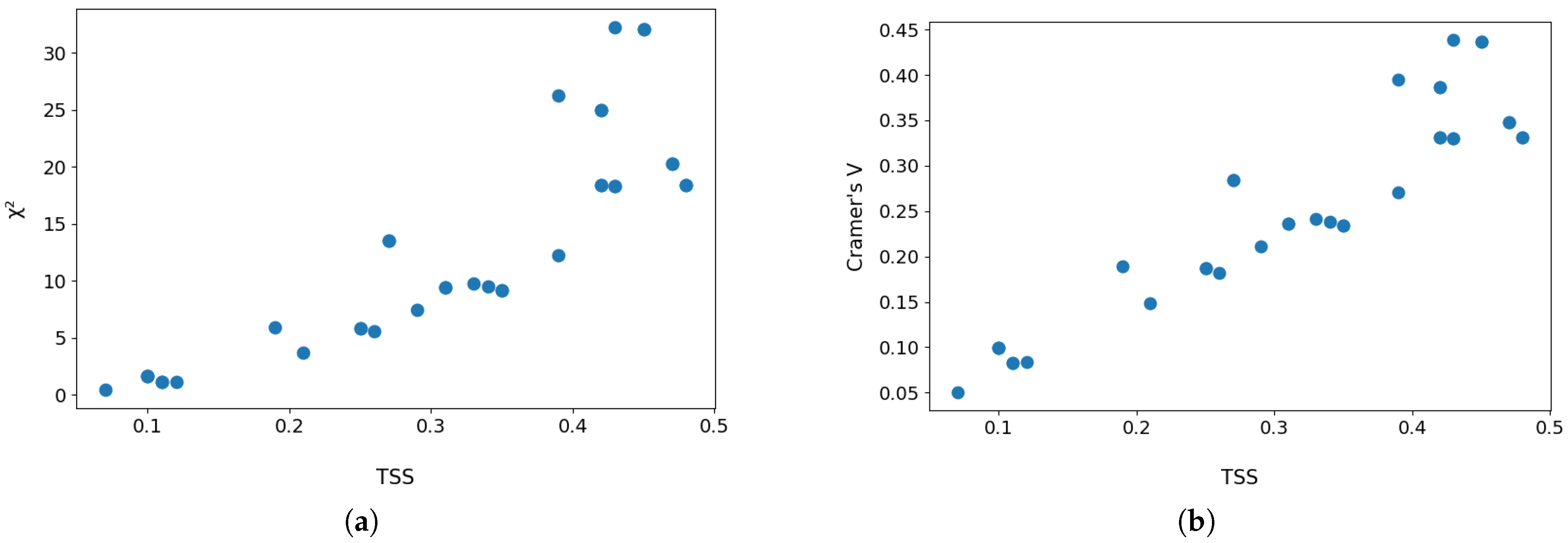
The obtained results (Table 3 and Table 4) indicate the proportionality of the $TSS$ values, the ${\chi }^2$ statistic values, and the Cramér’s V coefficient. These relationships are shown in Figure A1. However, the interpretation of the values is not equal.

Proportionality in each individual case does not imply a general linear relationship between ${\chi }^2$ and $TSS$. The values of the ${\chi }^2$ statistic fall within the range $[0,\infty )$. In a large sample, the higher the value of the ${\chi }^2$ statistic, the stronger the relationship between variables. Possible values of the $TSS$ metric are limited to the range $[-1,1]$, where one indicates correct classification of all cases (zero values of $FP$ and $FN$), i.e., a perfect fit, and 0 indicates randomness, no predictive capability. For negative values, the model often, and in the critical case (for $TSS=-1$), always, predicts the opposite of reality.

The relationship between the values of Cramér’s V coefficient and the values of the $TSS$ metric may be close to linear in the cases under consideration (Figure A1), but this does not follow from the definitions of both measures and does not constitute a general relationship. Both values are bounded by one, and their high values indicate strong agreement between the analyzed binary sequences. However, Cramér’s V coefficient only describes the strength of the relationship between variables and does not determine its direction, while $TSS$ additionally provides information about the nature of the classification. A $TSS$ value close to one indicates high classification ability and correct representation of event occurrence, while negative values indicate a tendency to classify oppositely to the observations. For this reason, Cramér’s V and $TSS$, despite providing similar information about the degree of agreement in the analyzed cases, are not equivalent measures.

Because there is no universally accepted qualitative scale for interpreting $TSS$ values, their assessment should always be conducted in the context of a specific research problem. The same TSS value can have different meanings depending on the characteristics of the analyzed catchment, the complexity of hydrological processes, the frequency of events, and the forecast horizon. In this study, sensitivity was assessed in particular, understood as the probability of low flow occurring in the event of a meteorological drought ($P(Q=1|M=1)$). However, a high sensitivity value does not equate to high overall classification efficiency measured using $TSS$. The $TSS$ index takes into account both sensitivity and specificity, thus enabling the assessment of the classification’s ability to simultaneously recognize the presence and absence of the studied phenomenon.

Moderate $TSS$ values with relatively high sensitivity values mean that low flows are correctly captured when they occur, but their absence can also be falsely predicted. Even with relatively small groundwater resources, short-term or less intense episodes of meteorological drought do not necessarily translate into low flows. One possible explanation for this situation is that runoff is partially sustained by groundwater recharge, limiting the short-term flow response to rainfall deficits. This means that $TSS$ alone does not fully reflect the nature of the relationship between the occurrence of meteorological drought and low flows, and its moderate values indicate limited effectiveness in distinguishing the absence of low flows from the occurrence of meteorological drought.

4. Discussion and Conclusions

Both standard meteorological drought indices and their short-term counterparts exhibit stronger correlations with low flows as the threshold flow increases, meaning their impact on river flow is more noticeable. This correlation is strongest for 3- and 6-month indices, indicating the significant role of increasing rainfall deficits over time. A similar conclusion was drawn from their research by [25], who noted that longer periods of SPI accumulation are most strongly correlated with the SSI-1 coefficient. The observed relationship may also be influenced by the hydrogeological characteristics of the catchment, which determine the way precipitation deficit propagates to runoff, including the dynamics of underground recharge and the associated delay in flow response—ref. [26] points out that there is no single indicator or single timescale that would be appropriate for catchments with different hydrological regimes.

Simultaneously, the asymmetrically arranged conditional probabilities $P(Q=1|M=1)$ and $P(M=1|Q=1)$ indicate that meteorological indices perform well in forecasting low flows (forward prediction) but less well in describing the causes of such flows (reverse detection). This indicates that not all low flows result directly from meteorological drought, but the risk of their occurrence increases significantly if a meteorological drought occurs. This observation is consistent with the results obtained by [24]. As the restrictiveness of the boundary flow threshold increases, the values of $P(M=1|Q=1)$ increase. Therefore, the more extreme the hydrological event, the more deterministic its relationship with meteorological conditions—drought indices—becomes. SPEI-based indices, which take into account both precipitation and estimated evapotranspiration, perform better on short timescales, emphasizing the importance of the latter phenomenon in the processes shaping low flows. A similar, and even broader, conclusion follows from the research by [28], where it was shown that the SPEI achieves higher correlation values with river flows and other variables characterizing the effects of drought than the SPI, which suggests that taking into account potential evapotranspiration may improve the representation of processes leading to the occurrence of hydrological drought.

SPI/SPEI-3–6 yield high probabilities of $P(Q=1|M=1)$, moderate values of $P(M=1|Q=1)$, and the highest of all determined $TSS$ values. Due to their stability, they can be useful in identifying conditions favorable to the occurrence of low flows, which coincides with environmental monitoring and seasonal prediction. Weekly scales (SPI-like indices) are characterized by greater variability in results, and a clear improvement in parameters is observed after taking into account the time shift of the binary sequences, i.e., examining the time after which the flow level will react (decrease) to meteorological conditions identified by SPI as drought. Taking this lag into account is crucial—the response of flow to meteorological conditions is not immediate, which is also confirmed by the conclusions in [26]. Due to the lower stability of the results, SPI-like indices may not provide as good predictive results as classical indices. Therefore, they cannot be used as the primary predictor of low flows. However, they can serve as a tool for capturing short-term dynamics and local responses, as a complementary tool for short-term warnings of the possibility of low water levels occurring or worsening.

The weekly timescale can be used where retention times are short and the catchment area responds quickly or not to rainfall. It appears that the weekly timescale may also be useful for local agricultural forecasts, due to the rapid response of soil and crops to rainfall deficits, even in situations where water is abstracted from a river for broadly defined economic purposes, and the predicted decrease in flow will prevent the negative consequences of the need to limit such abstraction.

Study Limitations

A limitation of the presented study is the evaluation of the proposed methodological framework based on a single case study catchment. Therefore, the obtained results should be considered a preliminary assessment of the approach’s applicability, not a full evaluation of its universality. In particular, the applicability of the proposed approach to catchments with different hydrological and physiographic characteristics, such as catchment size, topography, and water-retention properties, remains to be assessed. Further analyses, covering a larger number of catchments, are currently underway to assess the transferability of the proposed approach to other areas. An additional limitation of the study is the reduction in the analyzed events to a binary format, which allows for a direct assessment of the relationship between the occurrence of meteorological drought and low flows, but does not account for the intensity of the analyzed phenomena.