Effect of Blade Number on the Performance of a Small Francis Turbine for Rural Local Power Generation

Abstract

The increasing integration of distributed photovoltaics and wind power in rural grids necessitates enhanced peak-regulation flexibility, for which small Francis turbines offer a promising solution. This study investigates the effect of long–short blade number on the hydraulic performance and energy losses of a representative rural small Francis turbine under constant runner material usage. Five configurations (N = 13–17) are evaluated using SST-DES-based CFD simulations and entropy production theory. At the rated condition, the N = 15 configuration achieves the highest overall efficiency of 93.65%, exceeding N = 17 by 0.19 percentage points and N = 16 by 0.61 percentage points; at high-flow conditions, it maintains a similar advantage of approximately 0.26 percentage points over N = 17. In the low-flow region, the N = 17 scheme exhibits slightly higher efficiencies, with advantages of 0.85 percentage points over N = 15. The N = 15 scheme demonstrates more uniform velocity streamlines, gentler pressure gradients, and smaller high-entropy-production regions across all flow components, particularly at the rated point. Overall, N = 15 provides the best balance between rated-point performance and off-design stability and is recommended for engineering applications.

1. Introduction

Francis turbines are the most widely used hydro-energy-conversion devices in distributed small hydropower stations because of their broad applicable head range, high hydraulic efficiency, and stable and reliable operation. Against the background of the clean production strategy, rural small hydropower, with small Francis turbines as its core equipment, constitutes a high-quality clean-energy resource. According to the commonly adopted classification in the hydropower industry (e.g., IEC standards), small hydropower turbines typically refer to units with a rated output below 10 MW, while those below 1 MW are often classified as micro or mini hydro. Our study focuses on a representative rural small Francis turbine with a rated output of 105 kW, which falls well within this category. It can facilitate the local accommodation of distributed rural wind and photovoltaic power, safeguard the secure and stable operation of rural distribution networks, and optimize the rural energy-supply structure. As these units are increasingly required to smooth wind-photovoltaic output fluctuations and undertake peak-shaving and frequency-regulation duties, more stringent demands have been imposed on their full-operating-range performance. Therefore, research on the internal flow mechanisms and performance optimization of small Francis turbines is of direct engineering significance.

At present, the combination of CFD (Computational Fluid Dynamics) numerical simulation and model testing has become an important approach for investigating the flow characteristics and performance laws of Francis turbines. Mukherjee et al. [1] compared the effects of different CFD methodologies on unit-performance prediction; Zhu et al. [2] investigated the influence of turbulence models on prediction accuracy; Umar and Huang [3] analyzed flow characteristics under part-load conditions; Tiwari et al. [4,5] proposed multi-fidelity CFD analysis methods, covering both comparative methodology and parameter optimization; Zhang et al. [6] studied the influence of draft tube structural optimization on vortex suppression and energy dissipation; Wang et al. [7] analyzed entropy-production loss characteristics induced by the vortex rope in a Francis pump-turbine; and Favrel et al. [8] experimentally and numerically validated an optimized draft tube design. Together, these studies provide an important basis for performance analysis and optimization design of hydraulic turbines.

When a turbine deviates from its best-efficiency operating condition, unstable flow phenomena such as draft tube vortex ropes, inter-blade vortices, and pressure pulsations readily occur. Wang et al. [9], Li et al. [10], and Shahzer et al. [11] investigated cavitation and vortex-rope flow characteristics; Wang et al. [12] analyzed the evolution of draft tube vortex structures under part-load conditions; Trivedi et al. [13] and Favrel et al. [14] revealed the correlation mechanism between pressure pulsations and vortex-rope motion; Masoodi and Goyal [15] and Ramdani et al. [16] examined complex-condition flow features using unsteady simulation and large-eddy simulation, respectively; and Wen et al. [17] numerically investigated pressure pulsation and vortex characteristics in Francis turbines based on weak compressibility. These studies indicate that unstable flow structures constitute key factors affecting the safe and stable operation of units.

The number of runner blades is an important structural parameter governing the performance of Francis turbines. Lu et al. [18] studied the influence of blade number on draft tube flow and unit efficiency; Kumar et al. [19] analyzed the relationship between blade number and cavitation characteristics; and Dahal and Trivedi [20], as well as Sun et al. [21], investigated the effect of blade number on inter-blade vortex structures. For long–short blade structures, several experimental and numerical studies have been conducted to explore their effects on hydraulic performance [22,23,24]. Although existing studies have demonstrated the important influence of blade number and long–short blade arrangement on internal flow and hydraulic performance in Francis turbines, the understanding of energy-loss characteristics under full-flow conditions for different long–short blade-number configurations remains relatively insufficient.

Recent studies have specifically addressed the influence of splitter or long–short blades on Francis turbine performance. Jia et al. [22] experimentally demonstrated that long and short blades can improve unit efficiency and reduce pressure pulsation under off-design conditions. Song et al. [23] conducted multidisciplinary optimization of splitter blade geometry for high-head Francis turbines. Chen et al. [24] investigated the internal flow and pressure pulsation characteristics of a Francis turbine runner with long–short blades under varying guide vane openings, demonstrating improved flow stability and reduced pressure fluctuations. However, most existing studies focus on either a single blade-number configuration or limited operating conditions, and systematic investigations covering both low-flow and high-flow regimes remain scarce. In particular, the combined effects of long–short blade number on both runner performance and downstream draft tube flow have not been fully elucidated.

Accordingly, this paper takes a Francis turbine with long and short blades (also referred to as splitter blades in some studies) as the research object. Under the condition that the runner material usage remains basically unchanged, five blade-number configurations, N = 13, 14, 15, 16, and 17, are designed. CFD numerical simulations are then performed to analyze unit hydraulic efficiency, velocity streamlines, pressure distribution, and entropy-production-rate characteristics under different operating conditions. This reveals the effects of the number of long and short blades on hydraulic performance and energy loss in a Francis turbine, providing a reference for runner optimization design.

2. Research Object

2.1. Unit Parameters and Three-Dimensional Geometric Model Establishment

This study focuses on a representative rural small Francis turbine-generator unit. By establishing the full-passage geometric model and the numerical calculation model of the unit, the hydraulic performance and internal flow characteristics under different long–short blade configurations are investigated. The overall design parameters of the unit determine its operating range and hydraulic characteristics and provide the basis for subsequent simulation and comparative analysis. The main performance and structural parameters of the unit are listed in

Table 1. Main performance parameters of the turbine.

Parameters	Value	Unit
Rated output Pr	105	kW
Rated speed nr	1000	rpm
Rated flow rate Qr	0.39	m3/s
Rated head Hr	29.0	m
Number of runner blades N	13	——
Number of stay vanes Nsv	24	——
Number of guide vanes Ngv	24	——
Runner diameter D1	0.3	m

.

To comprehensively analyze the performance of the unit over the full-flow operating range, five typical operating conditions under the rated head were selected for the numerical simulations, as listed in

Table 2. Operating parameters under different head conditions.

Operating Condition	Head [m]	Rotation Speed [rpm]	Guide Vane Opening [°]
OC1	29.3	1000	10
OC2	29.3	1000	14
OC3	29.3	1000	20
OC4	29.3	1000	28
OC5	29.3	1000	34

. Each operating condition corresponds to a different guide vane opening. The selected conditions cover the low-flow, rated-flow, and high-flow ranges, thus fully reflecting the flow and performance variation characteristics under variable-load operation.

2.1.1. Overall Three-Dimensional Geometric Model of the Full-Passage Flow

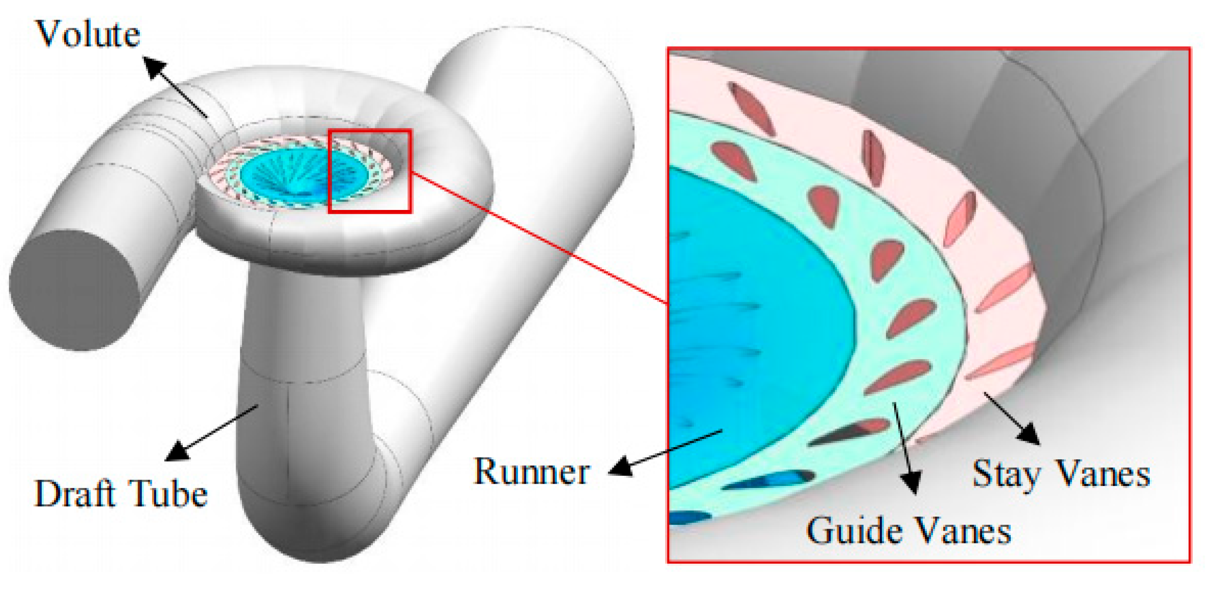
The complete flow passage of the unit is divided into four main components: the integrated volute–stay vane domain, the guide vane domain, the runner domain, and the draft tube domain. According to the prototype geometric dimensions, individual solid models of each component were established in the modeling software and then geometrically assembled. Key structures, including the volute tongue, guide vane airfoils, the spatial surfaces of the long and short blades, and the elbow and diffuser sections of the draft tube, were fully retained. The complete three-dimensional model of the turbine is shown in Figure 1.

2.1.2. Runner Geometric Models for Different Blade Schemes

The turbine runner investigated in this study adopts a combined long-and-short-blade structure. Compared with a conventional runner with only full-length blades, the long-and-short-blade arrangement can effectively optimize the flow passage structure, improve the non-uniform velocity distribution inside the runner, suppress adverse flow phenomena such as flow separation, secondary flow, and draft tube vortex ropes under low-load conditions, broaden the stable operating range of the unit and enhance the overall hydraulic stability. Based on this runner structure, a high-precision three-dimensional geometric model was established, in which the long-and-short-blade arrangement, blade-passage geometry, hub, and shroud were fully reproduced.

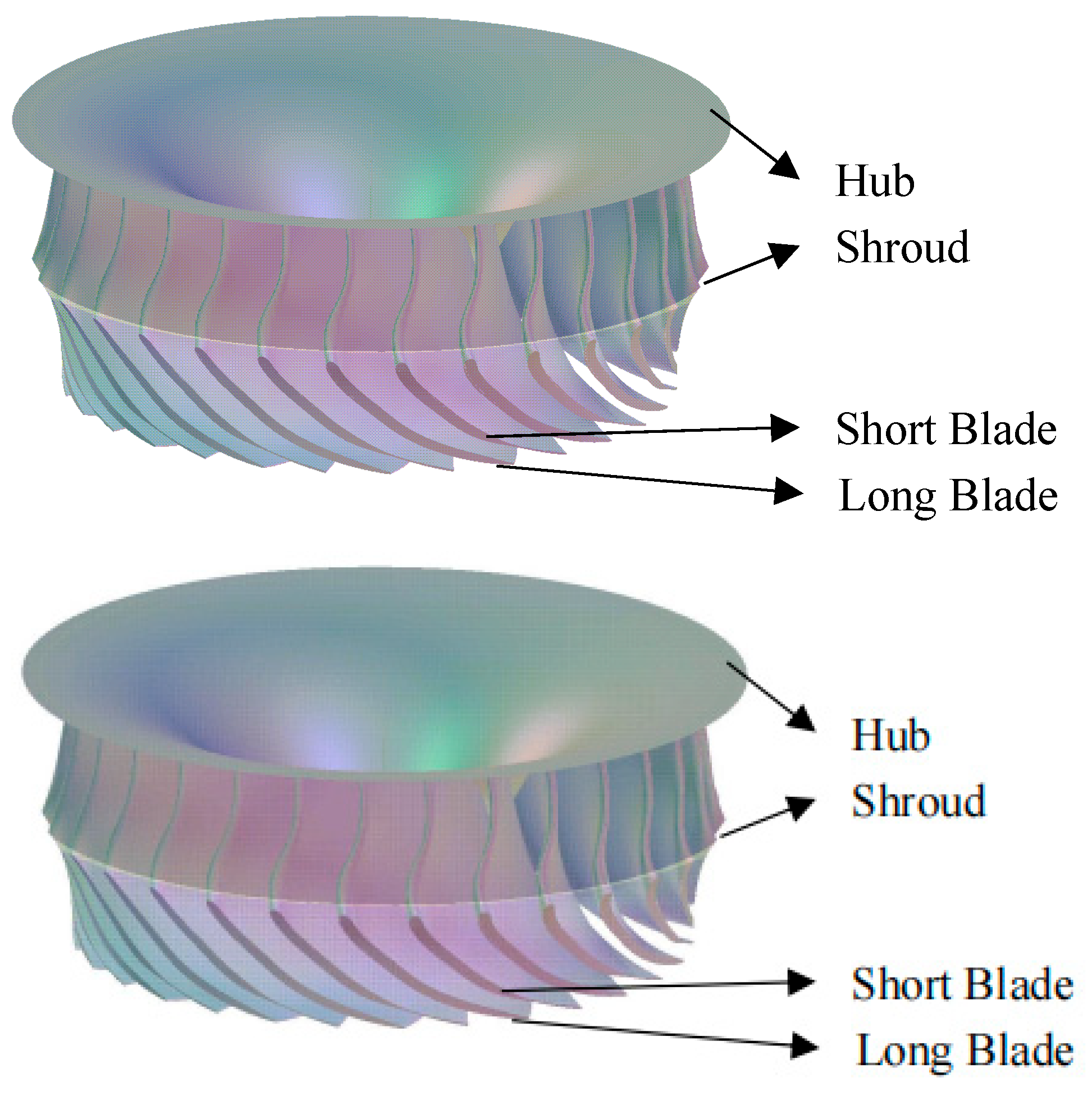
To investigate the effects of the number of long and short blades on the hydraulic performance and energy-loss characteristics of the Francis turbine, this study follows the single-variable principle. Taking the N = 15 long-and-short-blade configuration as the baseline model, other runner models with different blade numbers were constructed. The runner models are shown in Figure 2. While keeping blade profiles, installation angles, runner diameter, hub and shroud structures, and other parameters unchanged, five runner schemes with N = 13, 14, 15, 16, and 17 were generated by synchronously increasing or decreasing the number of long and short blades. In each scheme, blades were uniformly and symmetrically arranged in the circumferential direction to ensure structural consistency and the reliability of comparative results.

To ensure a fair comparison among the five blade-number configurations, the total runner material usage was kept approximately constant. Since all other components of the turbine (including the volute, stay vanes, guide vanes, and draft tube) have fixed dimensions, any change in the number of runner blades must be accompanied by an adjustment of blade thickness to maintain the overall runner size compatible with the fixed flow passage. Specifically, as the number of long–short blade groups was increased (from N = 13 to N = 17), the blade thickness was slightly reduced to keep the total blade volume close to that of the baseline N = 15 configuration; conversely, when the blade number was decreased, the blade thickness was slightly increased. This approach ensures that the performance differences observed among the schemes can be attributed primarily to the blade number and passage geometry, rather than to variations in material usage or runner size.

The N = 13 scheme contains two fewer groups of long and short blades than the baseline model and represents the scheme with the smallest blade number. After the blade number is reduced, the runner passage area increases and the ability of the blades to guide and constrain the flow weakens; this scheme is therefore used to analyze the flow-field structure and energy-loss characteristics under a relatively small blade number.

The N = 14 scheme contains one fewer group of long and short blades than the baseline model. Its blade density and passage area lie between those of the N = 13 and N = 15 schemes. This scheme can reveal the influence of a slight reduction in blade number on the internal flow and hydraulic performance of the runner.

The N = 15 scheme is used as the baseline model. With moderate blade spacing, it balances passage-flow capacity and flow-guiding capability and thus provides a reference for comparing schemes with different blade numbers.

The N = 16 scheme contains one additional group of long and short blades relative to the baseline model. Its blade density is increased, and the flow-guiding effect is further strengthened. This scheme is used to study changes in flow-field structure and energy loss after a slight increase in blade number.

The N = 17 scheme contains two additional groups of long and short blades relative to the baseline model and is the scheme with the largest blade number. Its blade arrangement is the densest and its passage area correspondingly decreases; thus, this scheme is used to analyze how increasing blade number affects flow characteristics, hydraulic loss, and operating performance.

In summary, with the N = 15 scheme as the baseline, comparative models with a gradient variation in blade number were constructed. In this way, the variation characteristics of runner internal flow structure, hydraulic loss, and unit performance under different long-and-short-blade configurations were systematically investigated, providing a theoretical basis for runner parameter optimization and performance improvement of Francis turbines.

2.2. Research Methodology

2.2.1. Governing Equations of Fluid Flow

The internal flow in a Francis turbine is a complex three-dimensional viscous turbulent flow, accompanied by abrupt velocity variations, flow separation, vortex shedding, energy dissipation, and other complex hydraulic phenomena. To accurately simulate the evolution of the flow field, the distribution of hydraulic loss, and the turbulence characteristics inside runners with different long–short blade configurations, numerical simulation based on computational fluid dynamics is required. The water flow in the turbine can be regarded as an incompressible viscous fluid at normal temperature. The flow is governed by the incompressible Navier–Stokes equations, with the continuity and momentum equations given as [2,25]:

$${\displaystyle \frac{\partial u}{\partial x}}+{\displaystyle \frac{\partial v}{\partial y}}+{\displaystyle \frac{\partial w}{\partial z}}=0$$

(1)

$$\rho \left(u{\displaystyle \frac{\partial u}{\partial x}}+v{\displaystyle \frac{\partial u}{\partial y}}+w{\displaystyle \frac{\partial u}{\partial z}}\right)=-{\displaystyle \frac{\partial p}{\partial x}}+\mu \left({\displaystyle \frac{{\partial }^{2}u}{\partial x^2}}+{\displaystyle \frac{{\partial }^{2}u}{\partial y^2}}+{\displaystyle \frac{{\partial }^{2}u}{\partial z^2}}\right)+\rho g_{\mathrm{x}}$$

(2)

$$\rho \left(u{\displaystyle \frac{\partial v}{\partial x}}+v{\displaystyle \frac{\partial v}{\partial y}}+w{\displaystyle \frac{\partial v}{\partial z}}\right)=-{\displaystyle \frac{\partial p}{\partial y}}+\mu \left({\displaystyle \frac{{\partial }^{2}v}{\partial x^2}}+{\displaystyle \frac{{\partial }^{2}v}{\partial y^2}}+{\displaystyle \frac{{\partial }^{2}v}{\partial z^2}}\right)+\rho g_{\mathrm{y}}$$

(3)

$$\rho \left(u{\displaystyle \frac{\partial w}{\partial x}}+v{\displaystyle \frac{\partial w}{\partial y}}+w{\displaystyle \frac{\partial w}{\partial z}}\right)=-{\displaystyle \frac{\partial p}{\partial z}}+\mu \left({\displaystyle \frac{{\partial }^{2}w}{\partial x^2}}+{\displaystyle \frac{{\partial }^{2}w}{\partial y^2}}+{\displaystyle \frac{{\partial }^{2}w}{\partial z^2}}\right)+\rho g_{\mathrm{z}}$$

(4)

The above governing equations are solved using the finite-volume method implemented in Ansys Fluent 2022 R1 (Ansys, Inc., Canonsburg, PA, USA). The mesh generation was carried out using Ansys ICEM CFD 2022 R1 (Ansys, Inc., Canonsburg, PA, USA).

2.2.2. Turbulence Model

The Reynolds number of the flow inside the turbine is in the range of approximately 1.6 × 10⁶ to 4.7 × 10⁶ (based on the mean flow velocity and the runner circumferential speed, respectively), indicating that the flow is in a fully turbulent state, with abundant irregular turbulent fluctuations and complex vortex structures. To accurately capture the energy dissipation caused by turbulent fluctuations and vortex-rope evolution inside the runner, and to maintain consistency with the turbulent kinetic energy k and specific dissipation rate ω involved in the entropy production rate formula, the shear stress transport–detached eddy simulation (SST-DES) model was adopted in this study.

The SST-DES model combines the accuracy of the SST k-ω model in simulating near-wall boundary-layer flow with the robustness of the k-ε model in far-field free shear layers. Through the DES method, it automatically switches to large-eddy simulation mode in separated flow regions. Consequently, this model can more reasonably simulate complex turbulent structures in hydraulic turbines, especially in flows with strong shear, vortex shedding, and large-scale separation.

Compared with the standard SST k-ω model, the SST-DES model offers two key advantages for the present study. First, the standard SST model, being a Reynolds-averaged Navier–Stokes (RANS) approach, tends to overly dissipate large-scale turbulent structures in regions of flow separation and vortex shedding, which are critical for understanding energy losses in Francis turbines. The SST-DES model overcomes this limitation by switching to a large-eddy simulation (LES) mode in regions where the grid is sufficiently fine, thereby resolving the unsteady vortex dynamics more accurately. Second, the entropy production analysis in this study relies on the accurate prediction of turbulent kinetic energy k and specific dissipation rate ω, particularly in the near-wall and separated flow regions. The SST-DES model retains the near-wall modeling capability of the SST k-ω model while improving the prediction of large-scale turbulence in the core-flow and wake regions, ensuring a more reliable entropy production estimation. For these reasons, the SST-DES model was selected as the most appropriate turbulence model for the present investigation.

The transport equations of the SST-DES model are based on the standard SST k-ω model. The transport equations for turbulent kinetic energy k and specific dissipation rate ω are expressed as follows:

$${\displaystyle \frac{\partial (\rho k)}{\partial t}}+{\displaystyle \frac{\partial (\rho u_{j}k)}{\partial x_j}}=P_{\mathrm{k}}-{\beta }^{*}\rho k\omega F_{\mathrm{DES}}+{\displaystyle \frac{\partial }{\partial x_j}}\left[(\mu +{\sigma }_{\mathrm{k}}{\mu }_{\mathrm{t}}){\displaystyle \frac{\partial k}{\partial x_j}}\right]$$

(5)

$${\displaystyle \frac{\partial (\rho \omega )}{\partial t}}+{\displaystyle \frac{\partial (\rho u_j\omega )}{\partial x_j}}={\displaystyle \frac{\gamma }{{\nu }_{\mathrm{t}}}}{P}_{\mathrm{k}}-\beta \rho {\omega }^2+{\displaystyle \frac{\partial }{\partial x_j}}\left[(\mu +{\sigma }_{\mathsf{\omega }}{\mu }_{\mathrm{t}}){\displaystyle \frac{\partial \omega }{\partial x_j}}\right]+2(1-F_1){\displaystyle \frac{\rho {\sigma }_{\mathsf{\omega }2}}{\omega }}{\displaystyle \frac{\partial k}{\partial x_j}}{\displaystyle \frac{\partial \omega }{\partial x_j}}$$

(6)

where ρ is the fluid density; u_j is the velocity component; P_k is the production term of turbulent kinetic energy; μ_t is the turbulent viscosity; F₁ is the SST blending function; ν_t = μ_t/ρ; and the remaining model constants take the standard SST-DES values.

DES switching is realized by introducing a length scale related to the local grid scale, defined as follows:

$$l_{\mathrm{k}\text{-}\mathsf{\omega }}={\displaystyle \frac{\sqrt{k}}{{\beta }^{*}\omega }}$$

(7)

$$l_{\mathrm{DES}}=\min (l_{\mathrm{k}\text{-}\mathsf{\omega }},C_{\mathrm{DES}}\Delta )$$

(8)

$$F_{\mathrm{DES}}=\max \left({\displaystyle \frac{l_{\mathrm{k}\text{-}\mathsf{\omega }}}{C_{\mathrm{DES}}\Delta }},1\right)$$

(9)

where Δ is the grid scale and C_DES = 0.61. When l_k-ω > _DESΔ, (s_DESΔ---C_DESΔ) the model enters the large-eddy simulation mode to resolve large-scale vortex structures; in the near-wall region, the Reynolds-averaged mode is retained to ensure boundary-layer prediction accuracy. The standard SST-DES model constants were used, and an automatic wall-function treatment was adopted in the near-wall region.The SST-DES model was implemented within the same CFD solver (Ansys Fluent 2022 R1). Pre-processing and solver settings were managed using Ansys CFD-Pre 2022 R1, and the simulations were executed through Ansys CFD-Solver 2022 R1.

2.2.3. Entropy Production Rate Theory

Entropy production in actual flow processes is a direct manifestation of the second law of thermodynamics. Irreversible flow processes increase system entropy, and energy dissipation simultaneously increases the internal energy of the fluid. The entropy production rate is an effective quantitative method for analyzing flow losses, as it can directly reflect the location and magnitude of energy loss induced by vortex structures. Based on velocity fluctuation characteristics, Kock and Herwig [25,26] proposed a model for calculating the local entropy production rate.

According to the production mechanism, entropy production can be divided into entropy production caused by dissipation effects and that caused by heat transfer effects. Each category can be further decomposed into a time-averaged viscous dissipation component and a turbulent fluctuation dissipation component. The time-averaged viscous dissipation term ${\dot{S}}_{\mathrm{p}\mathrm{r}\mathrm{o},\mathrm{D}}$ and the turbulent fluctuation dissipation term ${{\dot{S}}^{\prime }}_{\mathrm{p}\mathrm{r}\mathrm{o},\mathrm{D}}$ corresponding to dissipation effects are expressed as follows:

$${\dot{S}}_{\mathrm{pro},D}={\displaystyle \frac{\mu }{T}}\left[2{\left({\displaystyle \frac{\partial \overline{u}}{\partial x}}\right)}^2+2{\left({\displaystyle \frac{\partial \overline{v}}{\partial y}}\right)}^2+2{\left({\displaystyle \frac{\partial \overline{w}}{\partial z}}\right)}^2+{\left({\displaystyle \frac{\partial \overline{u}}{\partial y}}+{\displaystyle \frac{\partial \overline{v}}{\partial x}}\right)}^2+{\left({\displaystyle \frac{\partial \overline{u}}{\partial z}}+{\displaystyle \frac{\partial \overline{w}}{\partial x}}\right)}^2+{\left({\displaystyle \frac{\partial \overline{v}}{\partial z}}+{\displaystyle \frac{\partial \overline{w}}{\partial y}}\right)}^2\right]$$

(10)

$${{\dot{S}}^{\prime }}_{\mathrm{pro},D}={\displaystyle \frac{\mu }{T}}\left[2{\left({\displaystyle \frac{\partial u^{\prime }}{\partial x}}\right)}^2+2{\left({\displaystyle \frac{\partial v^{\prime }}{\partial y}}\right)}^2+2{\left({\displaystyle \frac{\partial w^{\prime }}{\partial z}}\right)}^2+{\left({\displaystyle \frac{\partial u^{\prime }}{\partial y}}+{\displaystyle \frac{\partial v^{\prime }}{\partial x}}\right)}^2+{\left({\displaystyle \frac{\partial u^{\prime }}{\partial z}}+{\displaystyle \frac{\partial w^{\prime }}{\partial x}}\right)}^2+{\left({\displaystyle \frac{\partial v^{\prime }}{\partial z}}+{\displaystyle \frac{\partial w^{\prime }}{\partial y}}\right)}^2\right]$$

(11)

The time-averaged term ${\dot{S}}_{\mathrm{p}\mathrm{r}\mathrm{o},\mathrm{C}}$ and the turbulent fluctuation term ${{\dot{S}}^{\prime }}_{\mathrm{p}\mathrm{r}\mathrm{o},\mathrm{C}}$ corresponding to heat transfer effects are calculated as follows:

$${\dot{S}}_{\mathrm{pro},\mathrm{C}}={\displaystyle \frac{\lambda }{T^2}}\left[{\left({\displaystyle \frac{\partial \overline{T}}{\partial x}}\right)}^2+{\left({\displaystyle \frac{\partial \overline{T}}{\partial y}}\right)}^2+{\left({\displaystyle \frac{\partial \overline{T}}{\partial z}}\right)}^2\right]$$

(12)

$${{\dot{S}}^{\prime }}_{\mathrm{pro},C}={\displaystyle \frac{\lambda }{T^2}}\left[{\left({\displaystyle \frac{\partial T^{\prime }}{\partial x}}\right)}^2+{\left({\displaystyle \frac{\partial T^{\prime }}{\partial y}}\right)}^2+{\left({\displaystyle \frac{\partial T^{\prime }}{\partial z}}\right)}^2\right]$$

(13)

The total entropy production is the sum of entropy production caused by dissipation and heat transfer effects:

$${\dot{S}}_{\mathrm{pro}}={\dot{S}}_{\mathrm{pro},\mathrm{D}}+{{\dot{S}}^{\prime }}_{\mathrm{pro},\mathrm{D}}+{\dot{S}}_{\mathrm{pro},\mathrm{C}}+{{\dot{S}}^{\prime }}_{\mathrm{pro},\mathrm{C}}$$

(14)

For incompressible flow with approximately constant temperature, the heat transfer entropy production terms are usually neglected, and the total entropy production can be simplified as:

$${\dot{S}}_{\mathrm{pro}}\approx {\dot{S}}_{\mathrm{pro},\mathrm{D}}+{\dot{S}}_{\mathrm{pro},{\mathrm{D}}^{\prime }}$$

(15)

The simplification is justified because the temperature variations in the present hydraulic turbine flow are negligible (the flow is essentially isothermal). For low-Mach-number water flows, the entropy production due to heat transfer is several orders of magnitude smaller than that due to viscous dissipation. According to Kock and Herwig [25], the error introduced by neglecting the heat transfer terms is typically less than 5% for incompressible flows with moderate temperature gradients. Wang et al. [7] also demonstrated that for hydraulic turbine applications, the simplified entropy production formula provides sufficiently accurate predictions of energy-loss distribution. Therefore, the simplified formula adopted in this study is considered appropriate for the present analysis.

Numerical simulation based on the Reynolds-averaged Navier–Stokes (RANS) method can solve only the time-averaged velocity field and cannot obtain the fluctuating velocity field directly. Therefore, this method cannot directly calculate the fluctuating entropy production. In this study, CFD simulations were performed using the SST-DES model, and the local entropy production rate E_p induced by velocity fluctuations was visualized according to:

$$E_{\mathrm{p}}={\displaystyle \frac{\rho \beta k\omega }{T}}$$

(16)

where k is the turbulent kinetic energy (m²/s²); T is the temperature (K); ρ is the working fluid density (kg/m³); β is the closure constant in the SST model, usually taken as 0.09; and ω is the turbulent specific dissipation rate (s⁻¹). Data post-processing and visualization were performed using Ansys CFD-Post 2022 R1 (Ansys, Inc., Canonsburg, PA, USA) and Origin 2024 (OriginLab Corporation, Northampton, MA, USA).

3. Numerical Model and Setup

3.1. Full-Passage Model Establishment

Using the small Francis turbine described in Section 2.1 as the research object, a full-passage three-dimensional geometric model was established, including the volute, stay vanes, guide vanes, runner, and draft tube. During modeling, the structural features of the unit were strictly retained, including the volute passage contour, guide vane profiles, the spatial surfaces of the long and short blades, and the elbow and diffuser sections of the draft tube. The runner adopts a combined long–short blade structure. Taking the N = 13 scheme (13 long blades and 13 short blades) as the baseline model, four additional comparative schemes with N = 14, 15, 16, and 17 were derived. In all schemes, only the number of long and short blades was synchronously increased or decreased, and the blade thickness was slightly adjusted according to the total runner blade weight. Other parameters, such as blade profile, installation angle, hub diameter, and shroud diameter, were kept unchanged to satisfy the single-variable principle.

3.2. Mesh Generation and Independence Verification

3.2.1. Mesh Generation Scheme

The components were meshed to enable CFD analysis. To accommodate the complex geometry, tetrahedral elements were mainly used; prism layers were generated in the near-wall regions; and pyramid and hexahedral elements were locally introduced in transition regions.

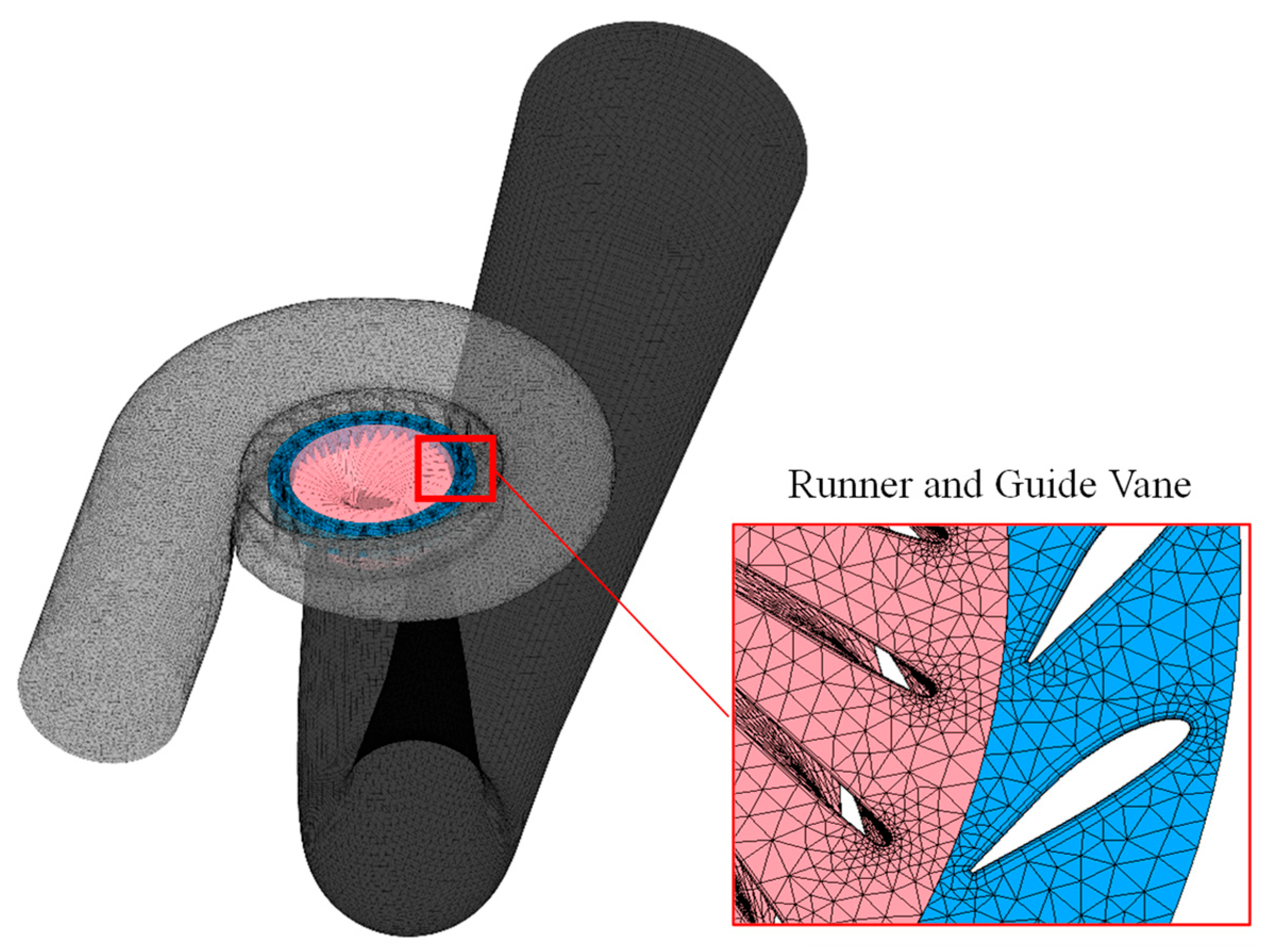
Figure 3 shows the full-passage assembly after meshing of the components. It presents the assembly relationship among the volute, guide vanes, runner, and draft tube. The component meshes are well connected at the interfaces; the overall mesh distribution is continuous; and no obvious distortion or abrupt size change is observed. The runner domain is a rotating domain, whereas the other components are stationary domains.

3.2.2. Mesh Independence Verification

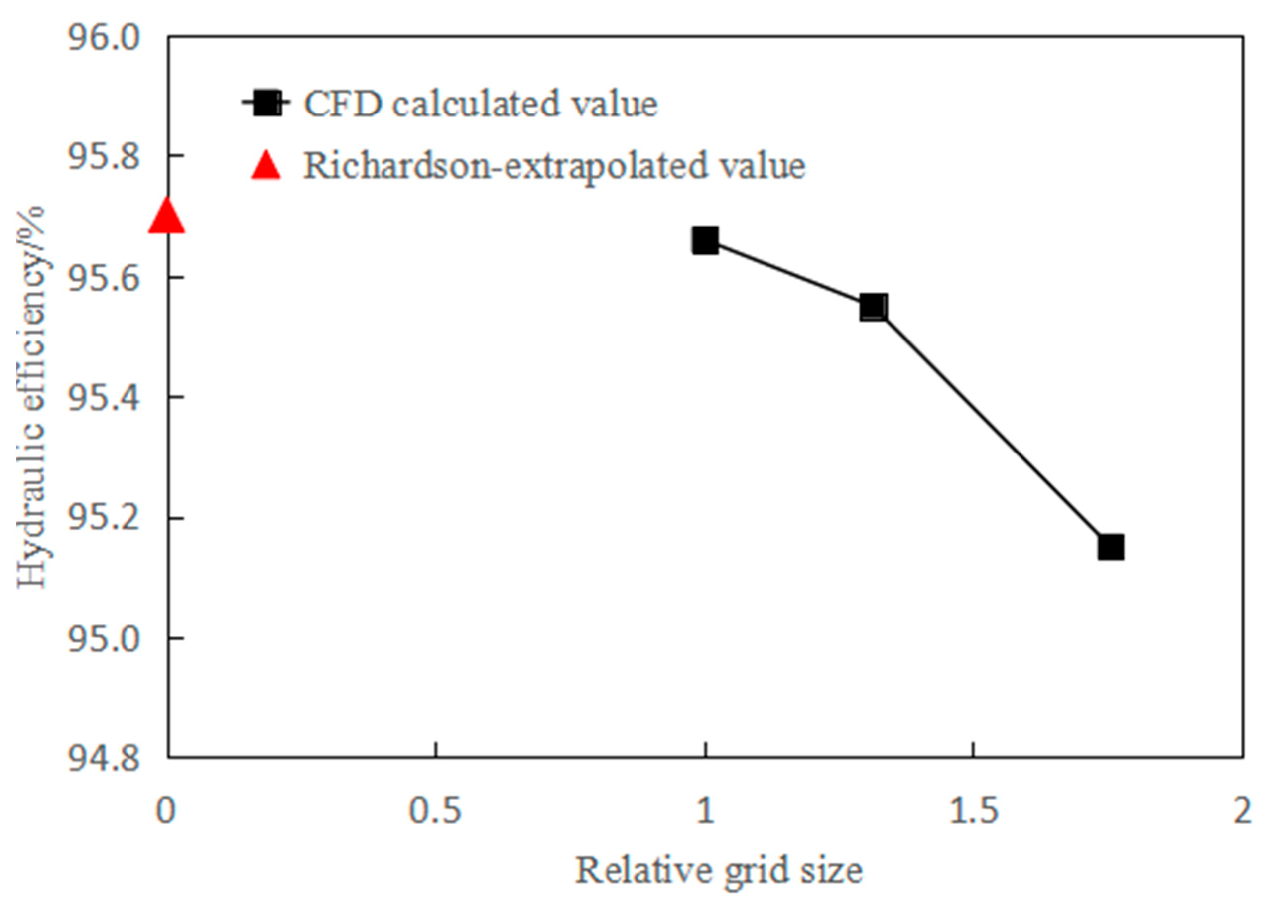
To ensure the accuracy and reliability of the numerical simulation results, the grid convergence index (GCI) method based on Richardson extrapolation [26,27] was used for mesh independence verification. Under an identical meshing strategy, local refinement method, and boundary-layer settings, three mesh schemes were generated by adjusting the global mesh size: a coarse mesh M1 with 1,039,080 elements, a medium mesh M2 with 2,710,485 elements, and a fine mesh M3 with 5,856,320 elements. Taking the hydraulic efficiency of the unit under the rated condition as the evaluation index, the corresponding efficiencies of the three meshes were 95.15%, 95.55%, and 95.66%, respectively. With mesh refinement, the efficiency gradually approached a stable value, indicating good numerical convergence.

Further calculation gave refinement ratios of 1.312 and 1.338 for the adjacent meshes, with corresponding GCI values of 0.43% and 1.57%, respectively. Both values satisfy the grid convergence requirement, and the errors remain at a low level. The results indicate that further mesh refinement exerts a minor influence on the calculated results, and the numerical model has good mesh independence. Considering both computational accuracy and cost, the medium mesh scheme with 2,710,485 elements was ultimately selected as the unified computational mesh for subsequent numerical simulations. The mesh independence verification results are shown in Figure 4. The final mesh numbers of the components are listed in

Table 3. Mesh numbers of the components.

Component	Mesh Node Number
Draft Tube	365,919
Volute and Stay Vane	423,617
Runner	1,567,283
Guide Vane	353,666
Total	2,710,485

.

3.3. Numerical Setup

The finite-volume method was used to discretize the governing equations, and the calculation mode was steady. The reference pressure was set to 101,325 Pa. The working fluid was clean water, with density ρ = 1000 kg/m³ and dynamic viscosity μ = 1.002 × 10⁻³ Pa·s. The turbulence model was the SST-DES model introduced in Section 2.2, and the entropy production rate formula was used for the subsequent analysis. Automatic wall functions were adopted near the walls.

The boundary conditions were set as follows. The volute inlet was specified as a mass-flow inlet (with the flow rate given according to the rated condition and a turbulence intensity of 5%). The draft tube outlet was set as a static pressure outlet with an average relative static pressure of 0 Pa. All solid walls were treated as no-slip smooth walls. The runner domain was defined as a rotating domain with a speed of 1000 r/min, whereas the other domains were stationary. Data transfer between rotating and stationary domains was realized through frozen-rotor interfaces. The governing equations were discretized using a second-order upwind scheme, and a pressure-velocity coupling algorithm was used. Convergence was considered achieved when the residuals of all equations were lower than 1 × 10⁻⁵ and when the monitored inlet total pressure, outlet static pressure, and runner torque became stable.

The frozen-rotor approach was adopted at the interface between the rotating runner domain and the stationary domains. This method was chosen to preserve the circumferential non-uniformity of the flow, particularly the blade wakes, which are essential for accurately capturing the unsteady interactions in the turbine. The frozen-rotor model demonstrated robust convergence in our simulations and has been successfully used in similar hydraulic turbine studies [10].

To explore the influence of blade number on turbine performance, the five typical operating conditions described in Section 2.1, covering low-flow, rated-flow, and high-flow ranges, were selected. Numerical simulations were conducted for the five long–short blade configurations with N = 13, 14, 15, 16, and 17. By comparing the hydraulic performance of each scheme and by taking OC5 as a representative condition for detailed comparison of flow-field structure, pressure distribution, entropy production loss, and draft tube flow pattern, the mechanisms by which blade number affects hydraulic characteristics and energy loss were revealed.

To ensure the statistical representativeness of the numerical results, all reported performance parameters (efficiency, power, head, and flow rate) were obtained by time-averaging over the last 5 runner revolutions after the solution reached the convergence criteria described above. This averaging procedure eliminates transient fluctuations associated with the unsteady flow features and ensures comparability across different blade-number configurations.

4. Results

4.1. Hydraulic-Performance Comparison of Different Long–Short Blade Schemes

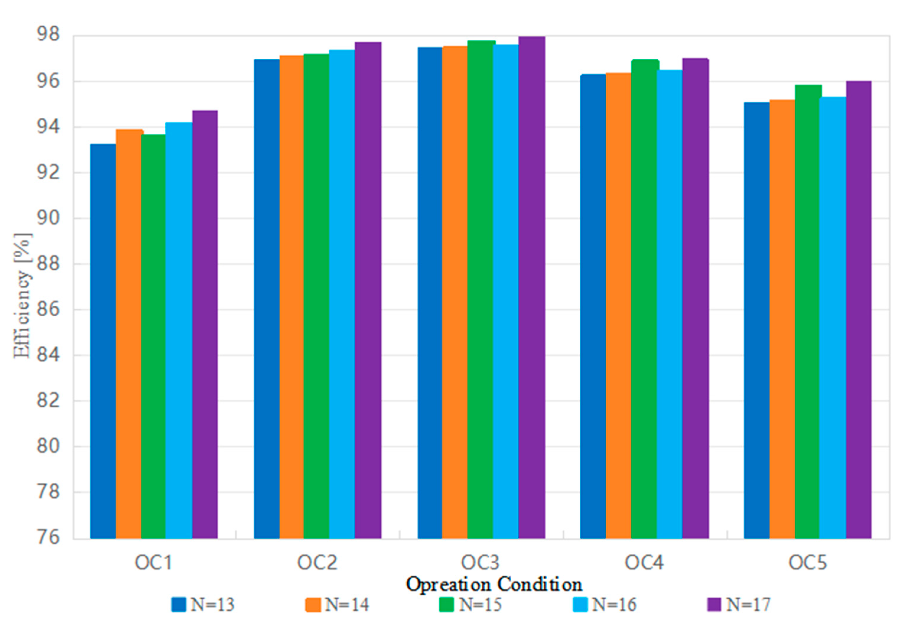
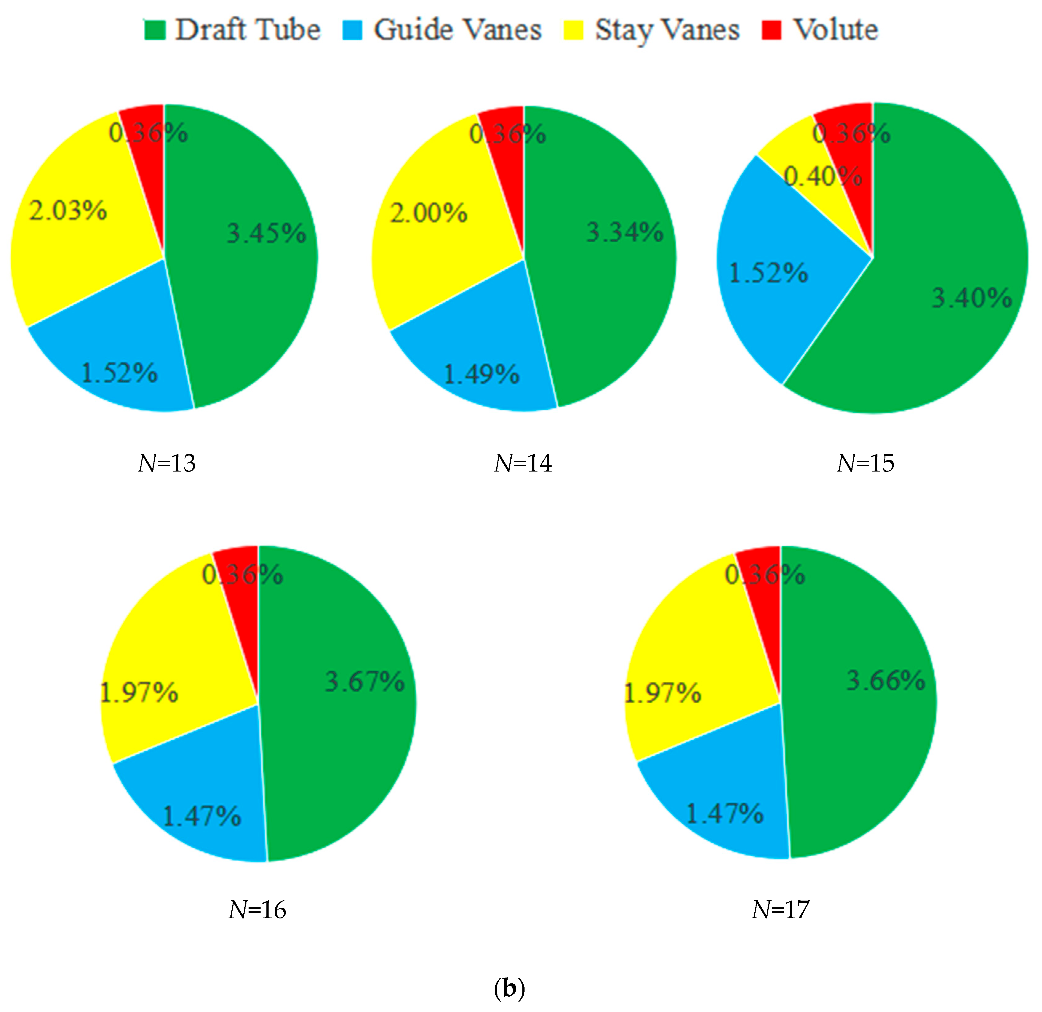
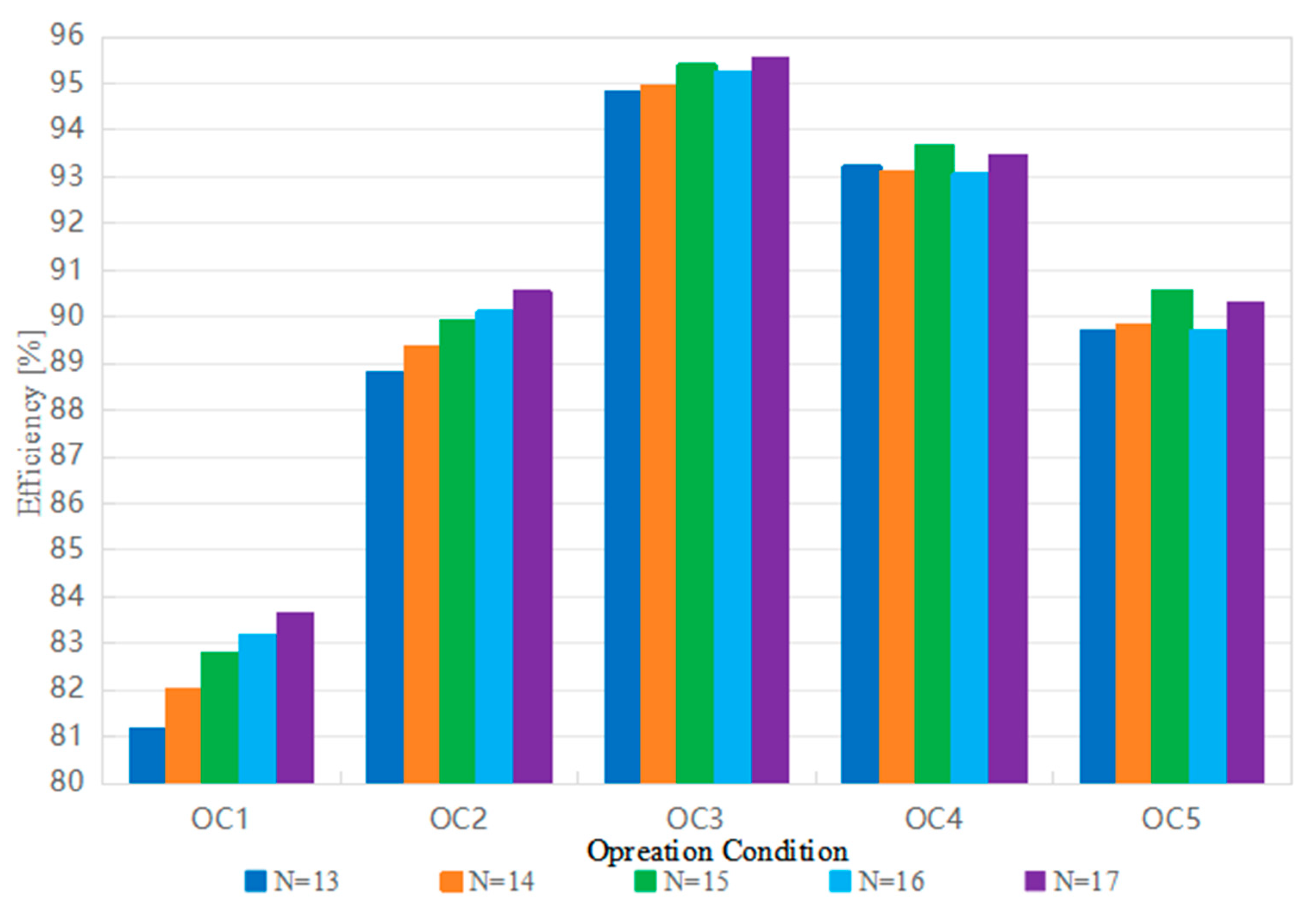
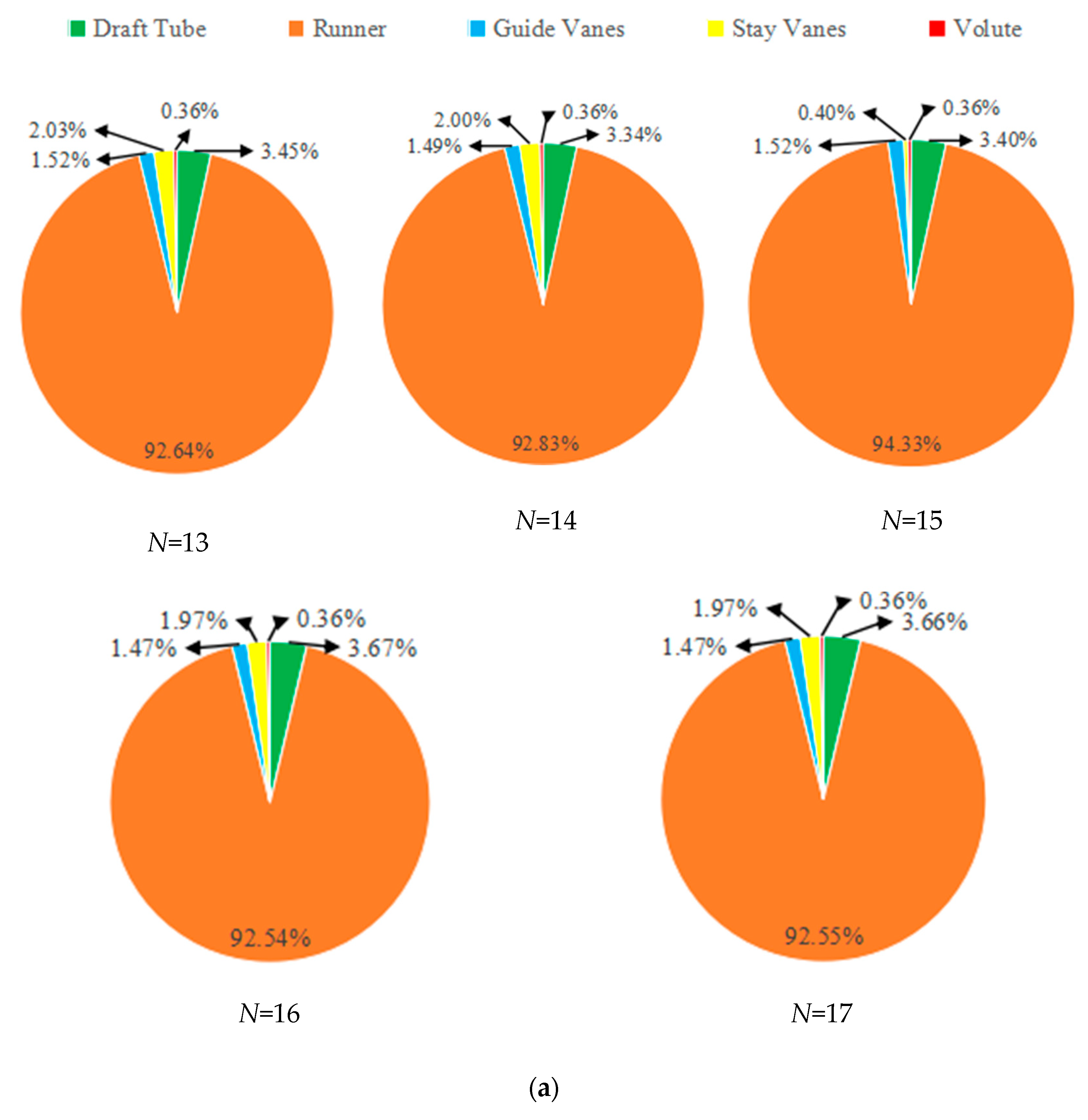
Combining the overall efficiency curve in Figure 5, the runner efficiency curve in Figure 6, and the energy-loss distribution of each component in Figure 7a (with a magnified view of the non-runner components in Figure 7b), it can be seen that different long–short blade configurations influence the hydraulic performance of the Francis turbine mainly in terms of efficiency level, loss allocation, and flow uniformity.

(1)

Consistency in the variation laws of overall and runner efficiencies.

Figure 5 and Figure 6 both show that the efficiency of each scheme follows a consistent trend with increasing flow rate: the efficiency is relatively low under low-flow conditions, increases rapidly as the flow rate increases, reaches a peak near the rated flow, and then decreases slightly and tends to stabilize in the high-flow range. This indicates that the overall unit performance is mainly controlled by the energy-conversion capability of the runner, whereas the guide vane system and draft tube modulate the efficiency variation.

In terms of efficiency level, the schemes show obvious operating-condition dependence. In the low-flow range, the N = 17 scheme has a slightly higher efficiency than the other schemes, indicating that increasing blade number can improve flow-confinement capability under low-load conditions. Under rated and high-flow conditions, however, the N = 15 scheme achieves the highest efficiency, followed by the N = 17 scheme; the N = 14 and N = 13 schemes are intermediate and relatively close, whereas the N = 16 scheme gives the lowest efficiency. These results indicate that an excessive blade number (N = 17), as well as the N = 16 configuration, is unfavorable for energy conversion under rated and high-flow conditions, whereas the N = 15 scheme performs best in this range.

In terms of efficiency level, the schemes show obvious operating-condition dependence. In the low-flow range, the N = 17 scheme has a slightly higher efficiency than the other schemes, indicating that increasing blade number can improve flow-confinement capability under low-load conditions. Under rated and high-flow conditions, however, the N = 15 scheme achieves the highest overall efficiency (Figure 5), followed by the N = 17 scheme; the N = 14 and N = 13 schemes are intermediate and relatively close, whereas the N = 16 scheme gives the lowest overall efficiency. In terms of runner efficiency (Figure 6), however, the N = 17 (purple) scheme slightly outperforms the N = 15 (green) scheme, indicating that the increased blade density improves flow guidance inside the runner passages. These results indicate that an excessive blade number (N = 17), as well as the N = 16 configuration, is unfavorable for energy conversion under rated and high-flow conditions, whereas the N = 15 scheme performs best in this range.

(2)

Differences between runner efficiency and overall efficiency.

As expected, the runner efficiency is generally higher than the overall unit efficiency, since the overall losses include contributions from the guide vanes and draft tube. The more meaningful comparison among the schemes is that although the N = 17 scheme shows a clearer advantage in runner efficiency, its advantage in overall efficiency is surpassed by the N = 15 scheme under rated and high-flow conditions. Similarly, the N = 16 scheme exhibits a moderate runner efficiency but the lowest overall efficiency, indicating that excessively dense blades (N = 17) or the specific N = 16 configuration may markedly increase losses in the guide vane and draft tube regions, thereby offsetting the gains in the runner.

Although the N = 15 scheme has no absolute advantage in runner efficiency alone, it provides the best overall efficiency under rated and high-flow conditions and maintains a high efficiency level over the full-flow range. This indicates a more balanced loss distribution throughout the entire passage and better system matching.

(3)

Characteristics of energy-loss distribution.

Figure 7a presents the overall spatial distribution of energy losses across all components for the different schemes. For all schemes, losses are mainly concentrated in the runner (more than approximately 92%), which is expected for hydraulic turbines. The more meaningful difference among the schemes lies in the distribution of the remaining losses: the N = 13 and N = 14 schemes show higher losses in the guide vanes and draft tube, whereas the N = 16 and N = 17 schemes exhibit increased runner losses. The N = 15 scheme achieves the most balanced distribution. To better visualize the differences among the schemes in the non-runner components, Figure 7b provides a magnified view of the losses in the guide vanes, draft tube, and other components.

From a scheme-to-scheme comparison, the N = 13 and N = 14 schemes have a slightly lower proportion of runner loss but relatively higher losses in the guide vane and draft tube regions, suggesting that fewer blades weaken flow control and cause energy to dissipate earlier in the upstream passage. In the N = 16 and N = 17 schemes, the runner loss proportion is higher; however, the guide vane and draft tube losses of the N = 16 scheme are abnormally high, resulting in its lowest overall efficiency. The guide vane loss of the N = 17 scheme also increases, but to a lesser extent than that of the N = 16 scheme.

By contrast, the N = 15 scheme has the highest and most concentrated runner loss proportion, approximately 94%, while its overall system loss is the lowest. This indicates that energy conversion is completed efficiently mainly in the runner, non-runner losses are minimized, and flow matching is the best.

(4)

Comprehensive conclusion.

Combining the efficiency curves and energy-loss distributions, it can be concluded that increasing blade number can improve low-flow efficiency. Nevertheless, the N = 16 scheme induces relatively large non-runner losses under rated and high-flow conditions, leading to a marked reduction in overall efficiency. Too few blades intensify flow separation and transfer system losses toward the guide vane and draft tube regions. The N = 15 scheme maintains a high efficiency level and small fluctuation over the full-flow range, exhibits a uniform loss distribution and the best flow matching, and therefore shows the most stable full-condition adaptability.

4.2. Flow-Field Comparison of Main Flow Passage Components

4.2.1. Flow-Field Comparison in the Guide Vane Region

Although the runner is located downstream of the guide vanes, the number of runner blades influences the upstream guide vane flow through the matching condition between the two components. The runner blade configuration determines the head-flow (H-Q) characteristic of the runner, which affects the pressure at the runner inlet and thus the back-pressure condition at the guide vane outlet. Consequently, the flow distribution and loss generation within the guide vane passages vary with the runner blade number, as shown in the following subsections.

• Velocity streamline comparison;

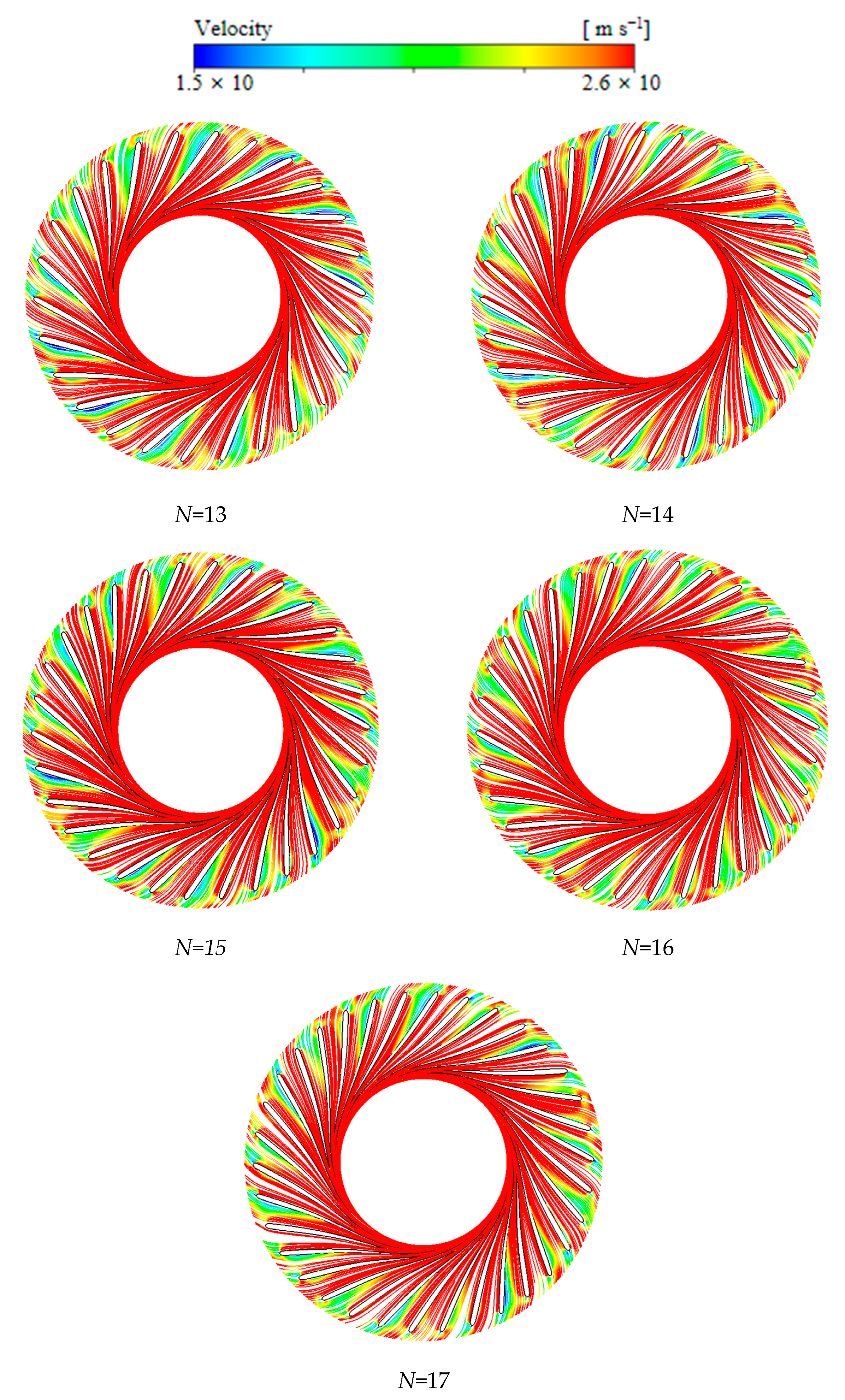
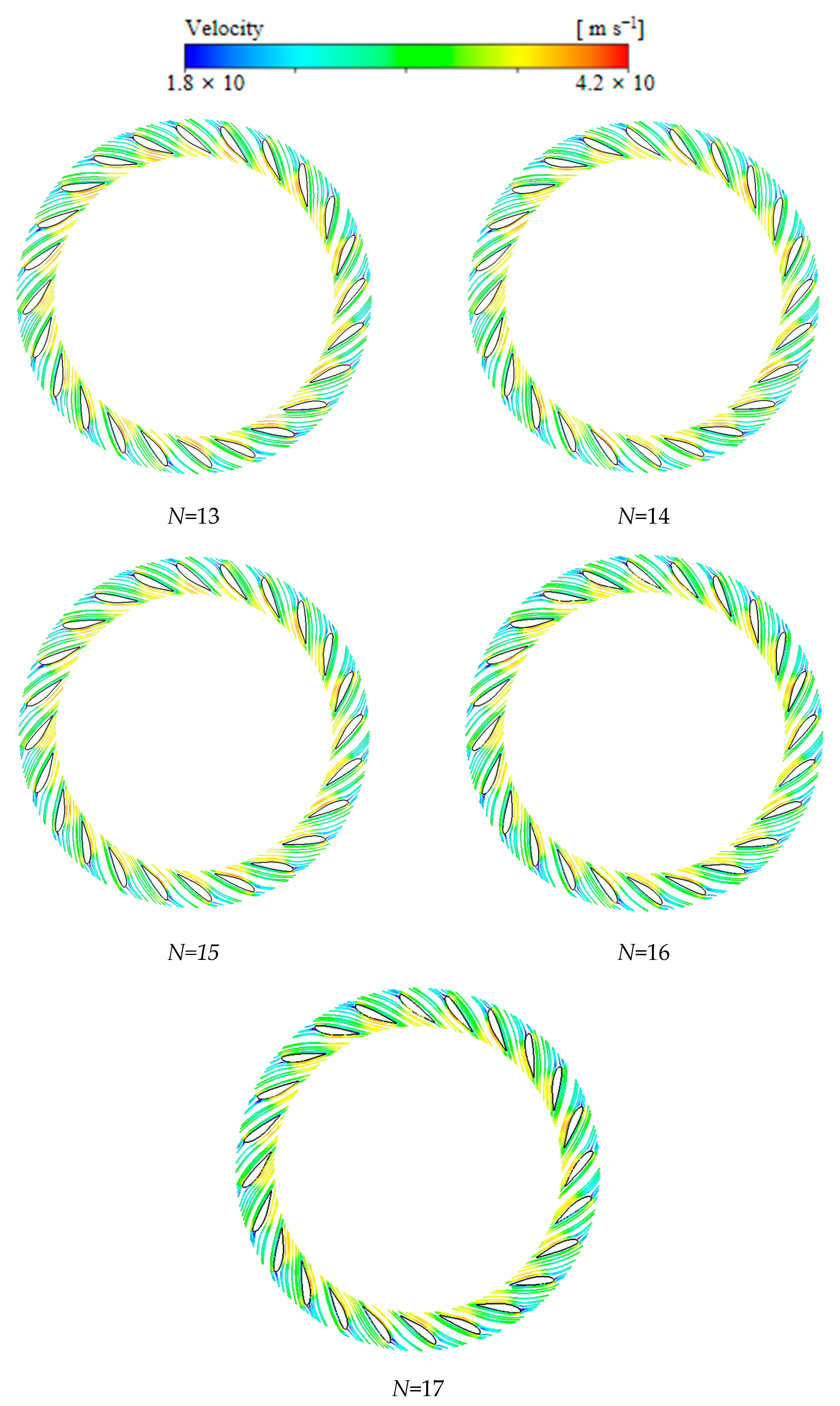
Figure 8 shows the velocity streamline distributions in the guide vane region under OC5 for different long–short blade schemes. It can be seen that, in all schemes, the flow can enter the runner region relatively smoothly through the guide vane passages, but the streamline uniformity differs. In the N = 13 scheme, local streamline deflection and clustering appear near the guide vane outlet, indicating poor flow stability. In the N = 14 scheme, streamline continuity is improved, but some regions with relatively large velocity gradients remain. In the N = 15 scheme, the streamlines are the most uniform, continuous, and smooth, and no obvious flow separation or backflow is observed. The outflow direction from the guide vanes matches well with the runner inlet, which is conducive to reducing hydraulic loss.

With a further increase in blade number, the outlet streamlines of the guide vane region in the N = 16 and N = 17 schemes remain generally regular, but local streamline crowding becomes more pronounced, producing larger velocity gradients and increasing local energy dissipation. Particularly in the N = 17 scheme, streamline compression is the most evident and flow resistance increases.

Overall, the N = 15 scheme produces the most uniform and stable flow in the guide vane region and provides the best flow-field quality, thereby supplying more uniform inlet conditions for the runner. This is consistent with its higher hydraulic efficiency.

2.

Pressure distribution;

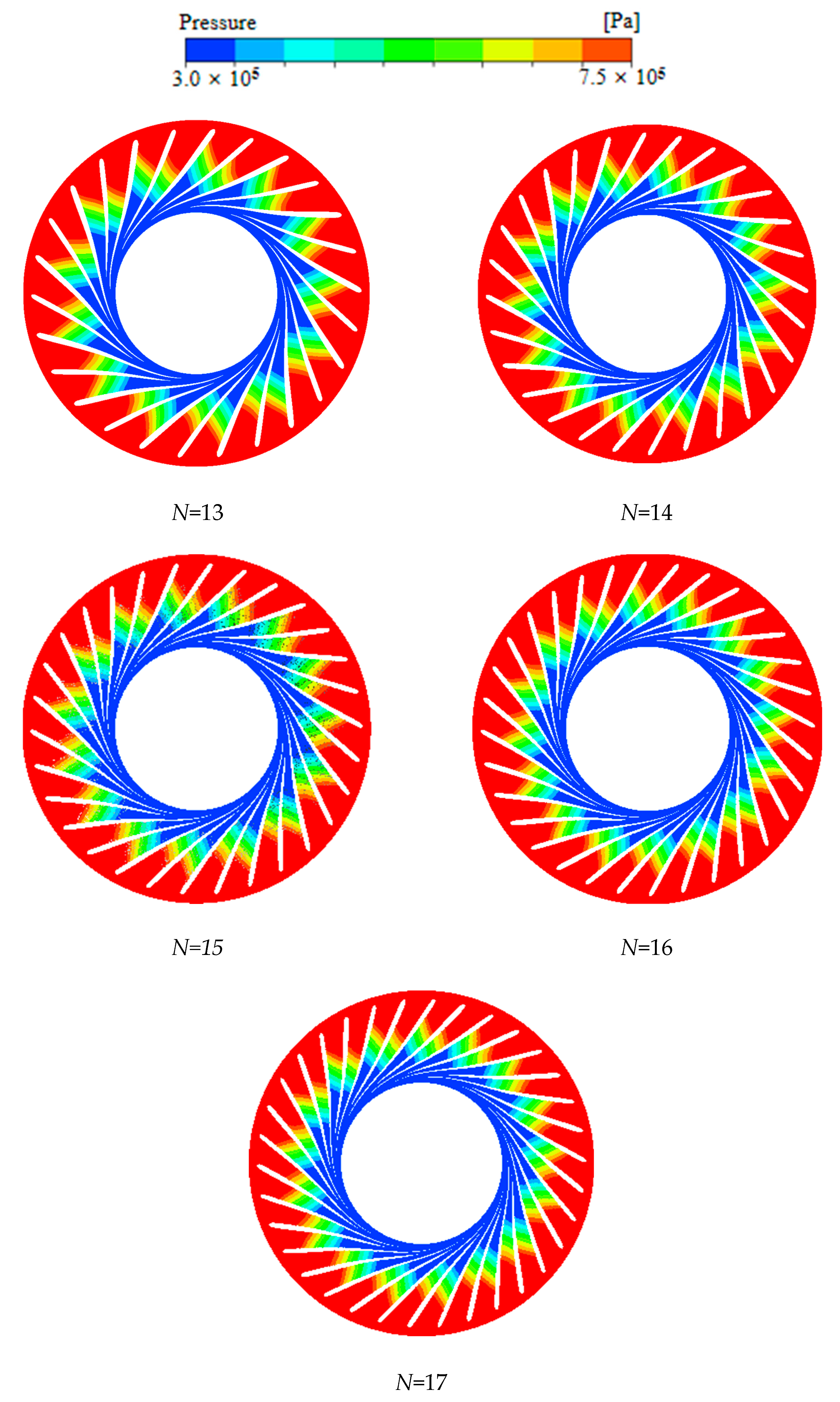
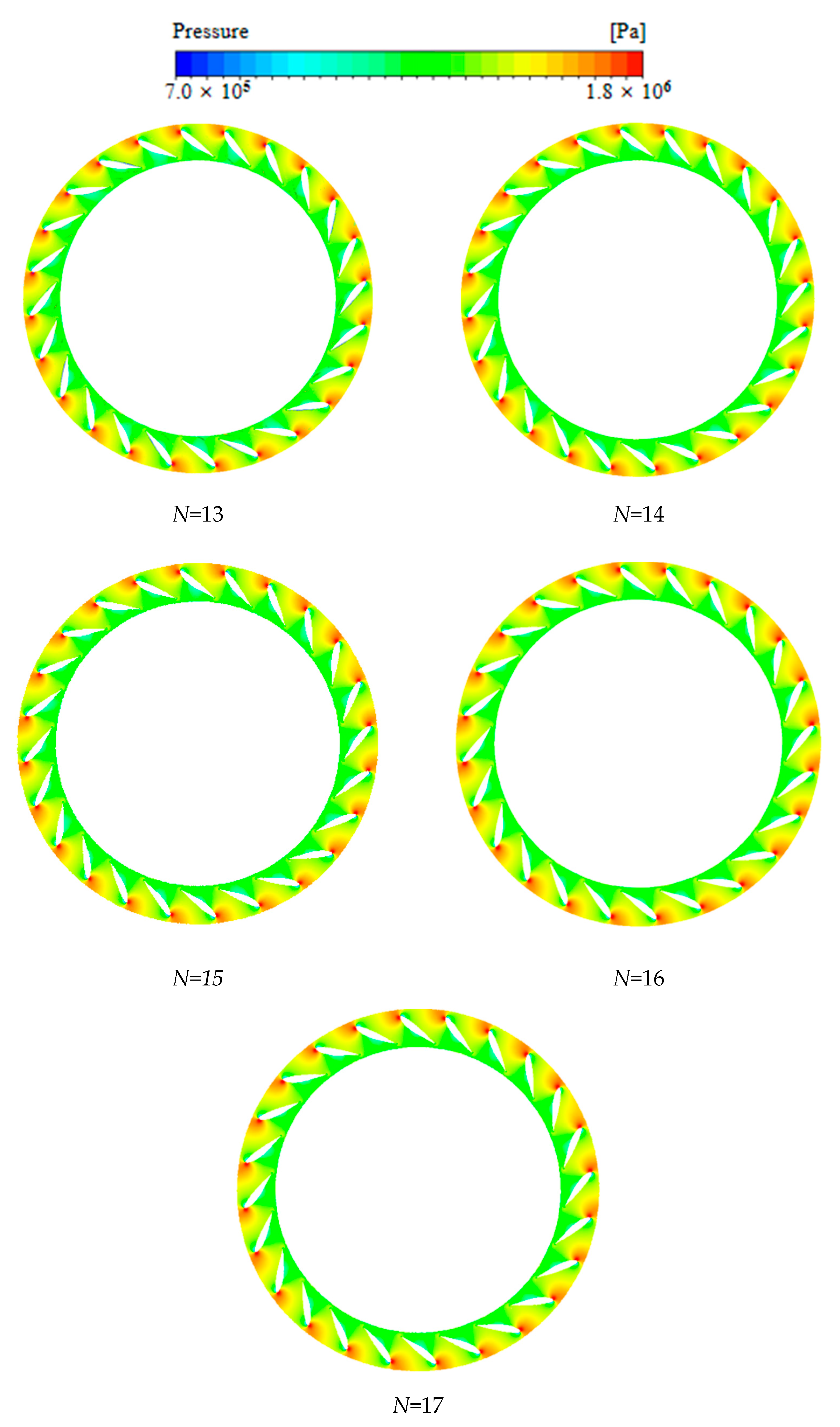
The Figure 9 shows that in all schemes, the guide vanes exhibit the typical pressure distribution pattern, with high pressure on the pressure side and low pressure on the suction side. The high-pressure regions are mainly concentrated near the guide vane inlet and the pressure surface, whereas the low-pressure regions are distributed along the suction surface and the trailing edge.

For the N = 13 scheme, the pressure distribution is less uniform, with a relatively large local low-pressure zone and evident pressure-gradient variation. The N = 14 scheme shows some improvement, although a certain degree of non-uniformity remains. The N = 15 scheme exhibits the most uniform pressure field, with smooth transitions between high- and low-pressure zones and small pressure gradients. This results in a more stable flow field at the guide vane outlet, which helps reduce hydraulic losses and improve the runner inlet conditions.

For the N = 16 and N = 17 schemes, the flow-guiding capability is enhanced due to the increased blade number; however, the local pressure gradients also increase. In particular, the N = 17 scheme shows a more concentrated interface between the high- and low-pressure regions, indicating increased flow resistance and friction losses.

In summary, the N = 15 scheme provides continuous and stable streamlines, a uniform pressure field, and satisfactory pressure recovery in the guide vane region. Combined with the subsequent entropy production analysis, this scheme is found to exhibit the lowest energy loss and the best overall hydraulic performance in terms of guide-vane flow quality.

3.

Entropy production distribution;

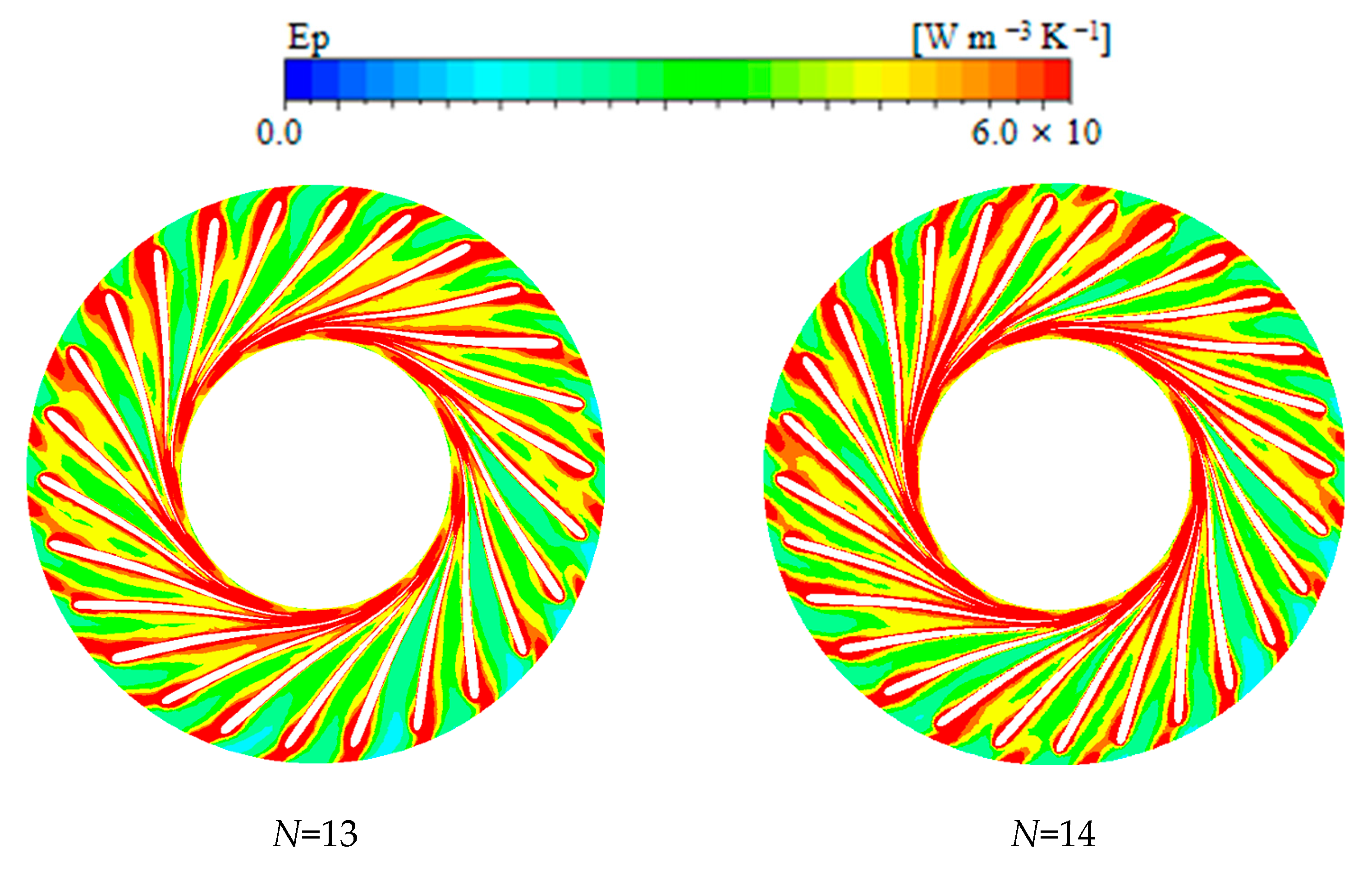
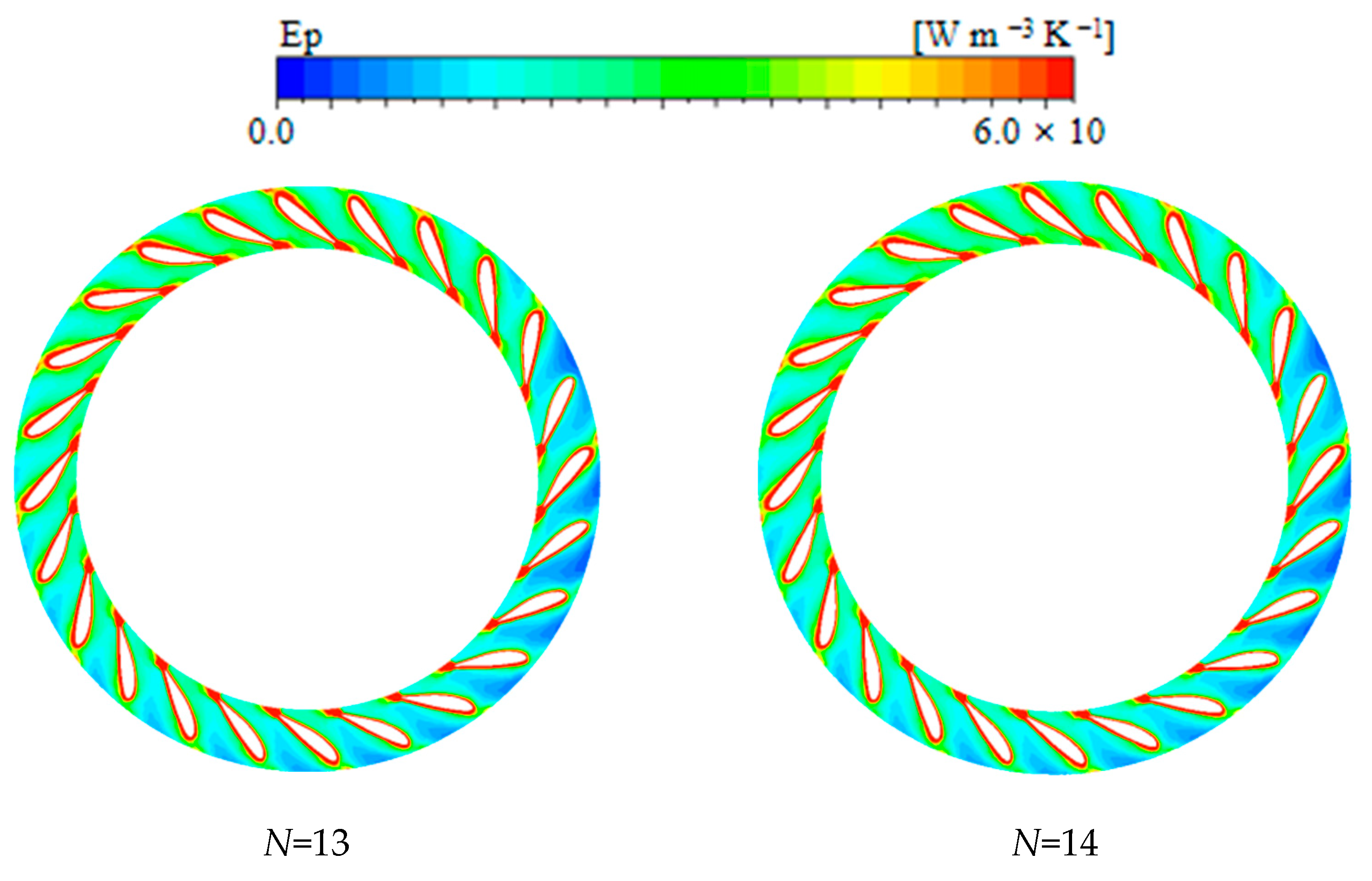
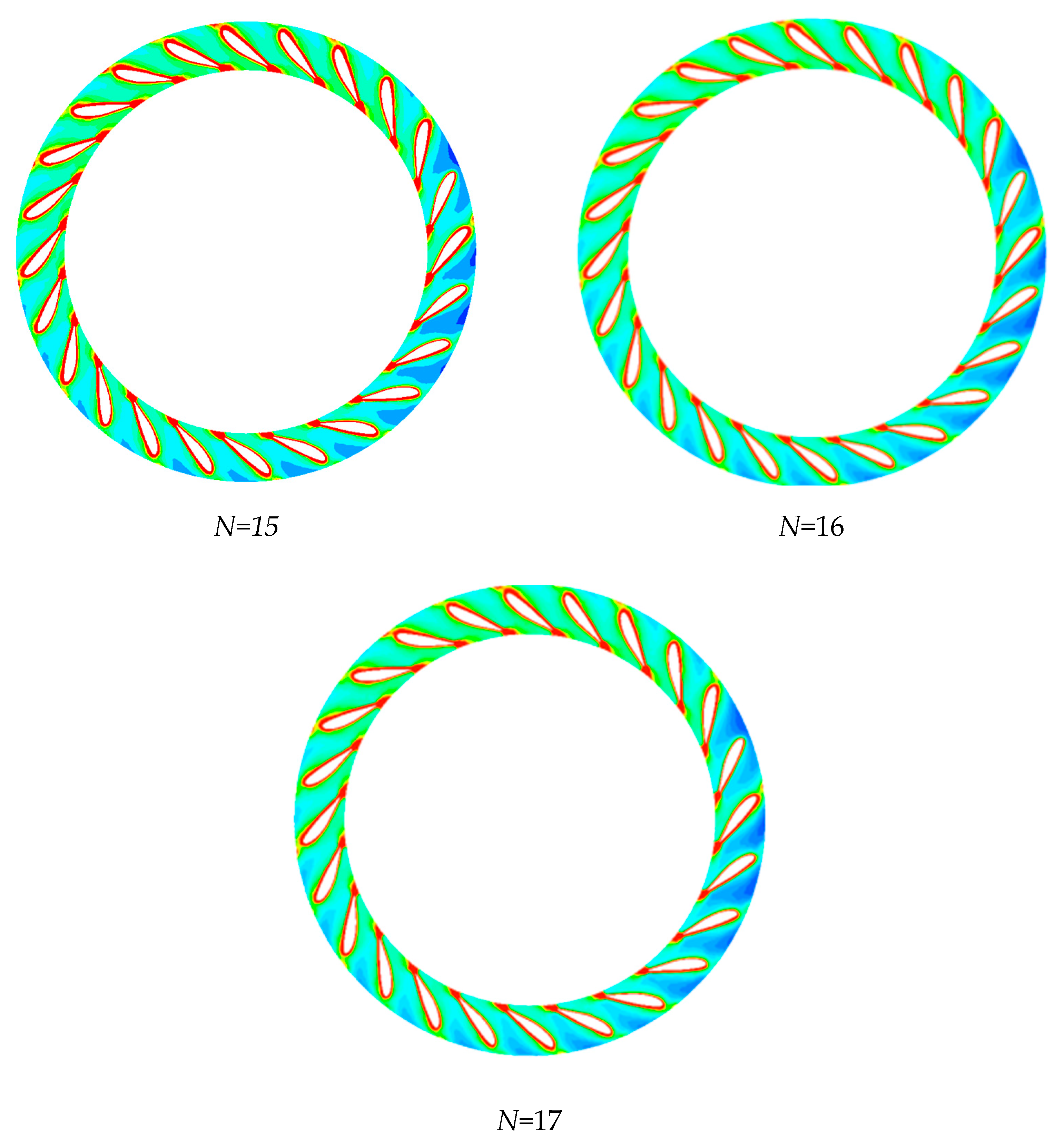
Figure 10 gives the entropy-production-rate contours in the guide vane region under OC5 for different long–short blade configurations. The high-entropy-production regions of all schemes are mainly concentrated near the guide vane suction surfaces and trailing edges. This is because, when the water passes through the guide vane passages, strong shear and boundary-layer development generate large velocity gradients and turbulent dissipation, thereby forming local zones of concentrated energy loss.

Compared among the different schemes, the entropy production distributions differ markedly. The N = 13 and N = 16 schemes have relatively large high-entropy-production regions with insufficiently concentrated distributions, indicating poor flow stability and strong local turbulent dissipation. In the N = 14 scheme, the high-entropy-production region contracts to some extent, but local entropy-production concentration remains, suggesting that flow uniformity still requires improvement. The N = 17 scheme exhibits a generally uniform entropy-production distribution, although certain high-entropy-production bands remain in local passages, reflecting increased friction loss under dense blade arrangement.

By contrast, the N = 15 scheme has the narrowest high-entropy-production region and the most uniform distribution within the passages. No obvious local entropy-production accumulation is observed. This indicates that the scheme effectively suppresses flow separation and turbulence development and reduces irreversible loss inside the guide vanes. Comprehensive analysis shows that the N = 15 scheme has the best guide vane flow quality and the lowest energy dissipation, in agreement with the velocity streamline and pressure distribution results.

4.

Entropy production comparison between near-wall and far-wall regions.

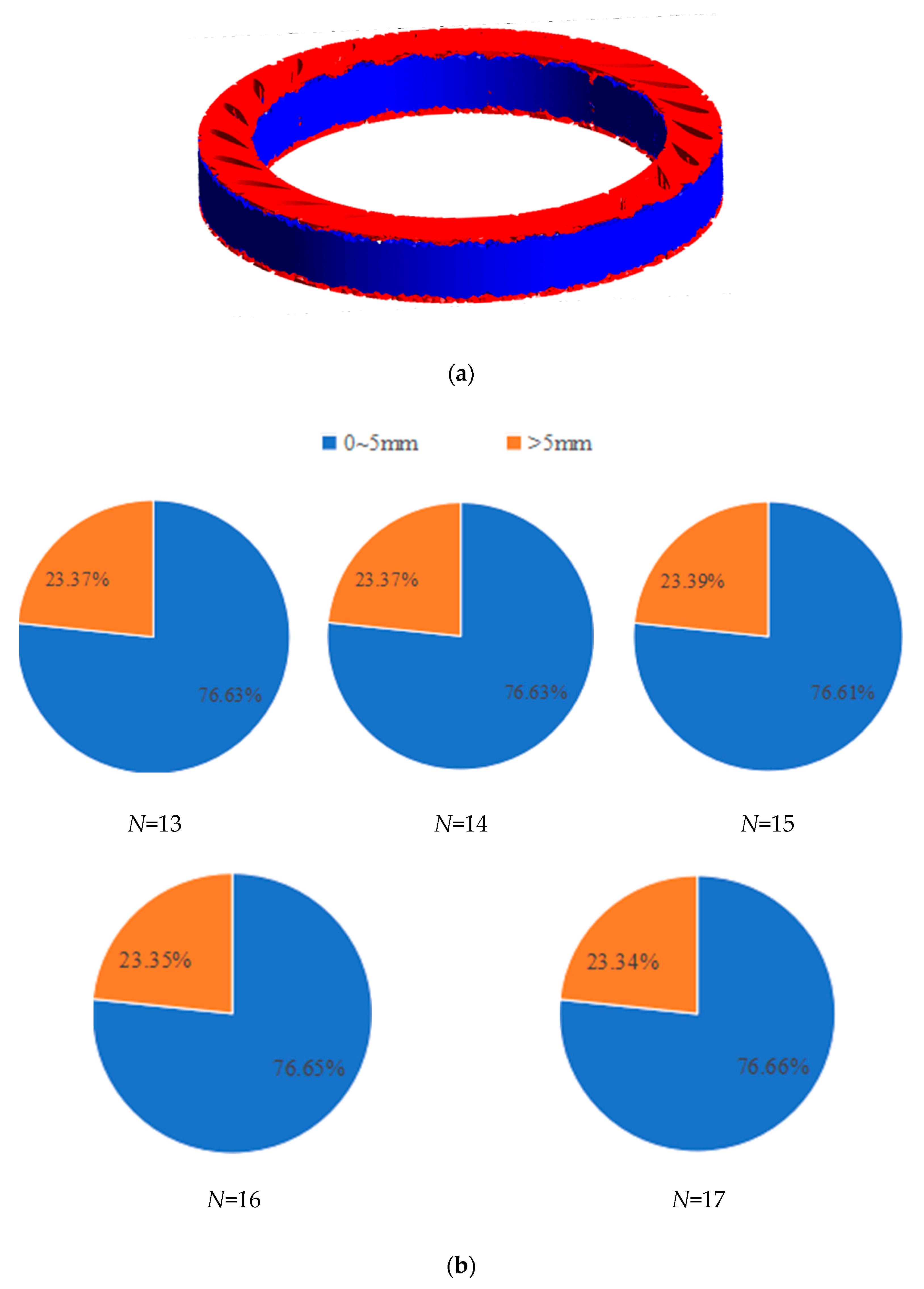
To further reveal the spatial-distribution characteristics of energy loss inside the guide vanes and quantify the entropy production contributions from near-wall and far-wall regions, the guide vane passages were divided, with the guide vane rotation center as the reference, into a near-wall region within 5 mm from the wall and a far-wall region beyond 5 mm. The threshold distance of 5 mm was chosen based on the estimated boundary-layer thickness at the guide vane outlet under the rated operating condition, which was determined from the local velocity profiles and near-wall grid resolution. To examine the sensitivity of the threshold selection, a preliminary analysis was performed by varying the threshold values by ±20%; the integrated entropy production values changed by less than 2%, confirming that the comparative conclusions among the different blade-number schemes are insensitive to the exact threshold choice. The same threshold criterion was applied consistently to all blade-number configurations to ensure comparability. Volume integration of the entropy production rate was then performed, and the results are shown in Figure 11b.

Figure 11b shows that entropy production in the guide vane region is mainly concentrated in the near-wall region for all schemes, accounting for approximately 76–77%, whereas the far-wall region accounts for approximately 23–24%. This indicates that wall shear and boundary-layer development dominate energy loss, and the near-wall region is the primary contributor to entropy production.

As expected for turbulent wall-bounded flows, entropy production in the guide vane region is mainly concentrated in the near-wall region for all schemes, accounting for approximately 76–77%, whereas the far-wall region accounts for approximately 23–24%. This confirms the physical consistency of our simulations. The more meaningful comparison among the schemes is presented below, where the differences in entropy production distribution between near-wall and far-wall regions are analyzed across the five blade-number configurations.

Comparing different blade-number schemes, certain differences exist in the allocation of entropy production between near-wall and far-wall regions. In the N = 13 scheme, the near-wall proportion is 76.63%, while the far-wall proportion is relatively high, indicating that when the blade number is small, flow diffusion is stronger and energy dissipation exists to some extent in the non-wall region. In the N = 14 scheme, the near-wall proportion increases slightly and far-wall loss decreases, suggesting improved flow-confinement capability. In the N = 15 scheme, the near-wall proportion is about 76.61%, which is at an intermediate level, but its far-wall entropy production is the most uniformly distributed, with no obvious local concentration. This indicates a more stable flow structure and a more reasonable energy-loss distribution. In the N = 16 scheme, the near-wall proportion is about 76.65%, slightly higher than those of the N = 13 and N = 14 schemes, implying enhanced wall-friction effects after the blade number is further increased. In the N = 17 scheme, the near-wall proportion is the highest, about 76.66%, indicating that dense blade arrangement strengthens wall shear and further increases friction loss in the near-wall region.

Although the differences in the near-wall entropy production proportions are small, they still reflect the influence of blade number on loss distribution inside the guide vanes. With too few blades, non-wall-region loss becomes more evident; with too many blades, wall-friction loss is intensified. Between these two tendencies, the N = 15 scheme achieves a better balance. Its entropy production distribution is more uniform, local energy dissipation is weaker, and its flow-organization capability is superior. Thus, in terms of entropy production control and distribution uniformity, the N = 15 scheme performs best, verifying its better guide vane flow quality and hydraulic-performance advantage.

It should be noted that the differences in entropy production proportions among the schemes are small (within 0.1 percentage point). However, the trends are systematic and consistent across all operating conditions. The grid independence study confirmed that the numerical uncertainty is well below the observed differences, and all configurations were evaluated using identical mesh topology and integration methods. Therefore, the observed trends are considered physically meaningful and reliable.

4.2.2. Flow-Field Comparison in the Runner Region

• Velocity streamline comparison;

Figure 12 shows the velocity streamline distributions in the runner domain under OC5 for different blade-number schemes. It can be seen that a distinct rotating-flow structure is formed inside the runner in all schemes, but the streamline-distribution characteristics differ. The N = 13 scheme maintains a relatively regular streamline pattern without obvious flow separation or recirculation, although the local streamline distribution is not sufficiently uniform. In the N = 14 scheme, the streamlines are less uniform compared with the N = 15 scheme, suggesting relatively stronger local velocity gradients. The N = 16 and N= 17 schemes maintain generally complete rotating-flow structures, although some local non-uniformities in the streamline distribution are observed compared with the N = 15 scheme.

By comparison, the velocity streamline distribution of the N = 15 scheme is the most uniform. The streamlines develop continuously and smoothly along the passages, the rotating structure remains complete, and no obvious streamline clustering, separation, or disorder is observed. This indicates that the scheme can effectively improve the internal flow state of the runner, enable the fluid to pass through the blade passages more smoothly, weaken the generation of local vortices and secondary flow, and thereby reduce flow loss while improving energy-transfer efficiency and flow-field stability.

Comprehensive analysis indicates that the N = 15 scheme has better flow-organization capability and flow-field uniformity, and its internal flow state is superior to those of the other schemes. This result is consistent with the low-loss characteristics obtained from the subsequent entropy production analysis, further demonstrating the favorable hydraulic performance of the N = 15 scheme.

2.

Pressure distribution;

Figure 13 shows the pressure contours in the runner region under OC5 for different blade-number schemes. In all schemes, the runner blades exhibit the distribution characteristic of high pressure on the pressure side and low pressure on the suction side. High-pressure regions are mainly located near the blade inlet and pressure surface, whereas low-pressure regions are concentrated on the suction surface and outlet region. This is consistent with the energy-conversion law inside the runner.

In the N = 13 scheme, because the blade number is relatively small, the surface-pressure distribution on the blades is less uniform and the local low-pressure region is relatively large. The N = 14 scheme shows improved pressure distribution, but some concentration of pressure gradient remains. In the N = 15 scheme, the pressure field is the most uniform; transitions between high- and low-pressure regions are smooth, and the pressure distributions among passages are highly consistent, indicating a relatively stable flow state. In the N = 16 and N = 17 schemes, the flow-guiding effect of the blades is strengthened as the blade number increases, but local pressure gradients also increase. This is especially evident in the N = 17 scheme, reflecting increased flow resistance and additional loss.

Comprehensive comparison shows that the N = 15 scheme has the most uniform pressure distribution and the most reasonable pressure gradient in the runner region. Combined with the velocity streamline and entropy production results, this scheme exhibits better flow quality and comprehensive hydraulic performance.

3.

Entropy-production distribution;

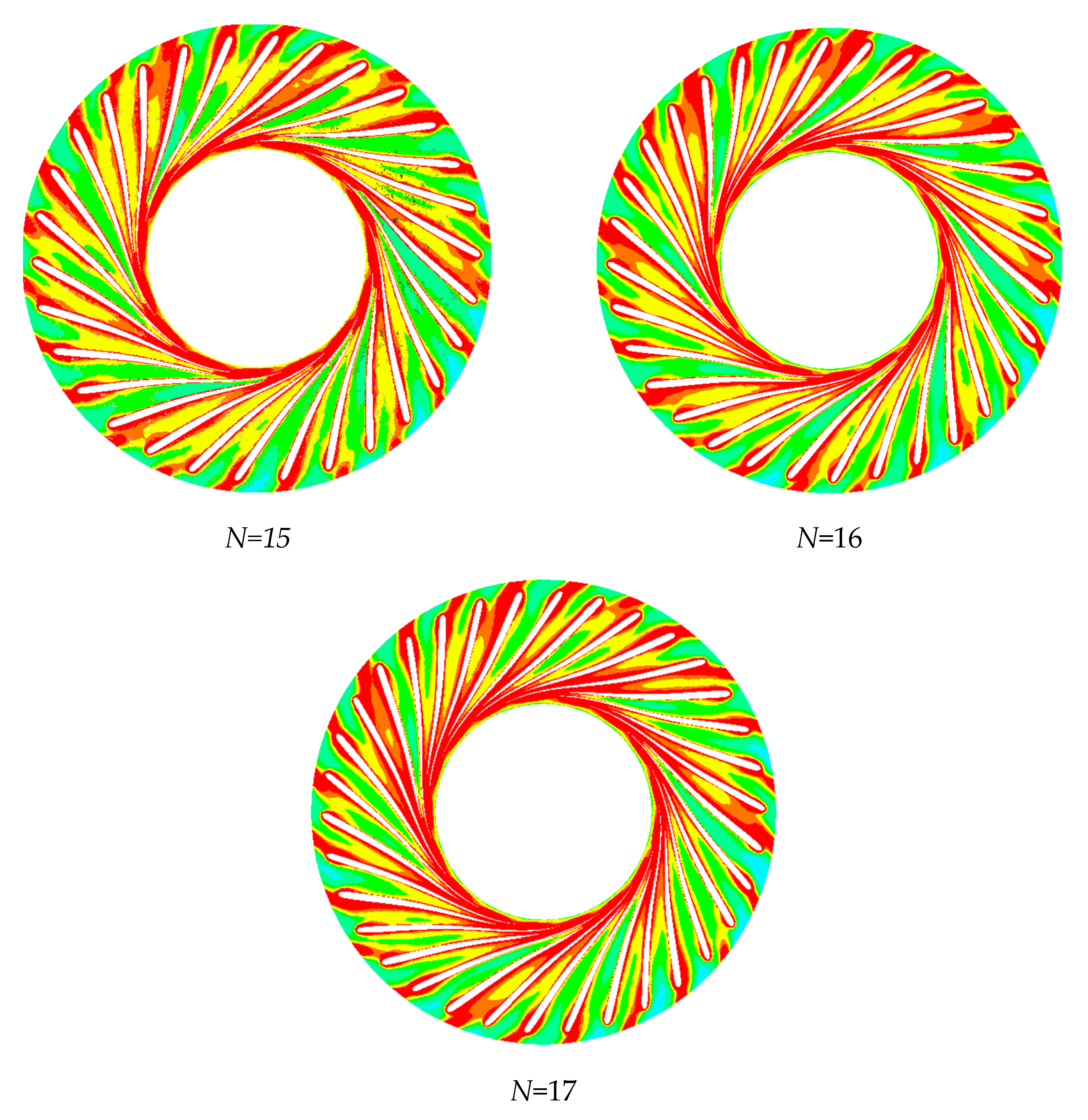
Figure 14 shows the entropy-production-rate contours in the runner region under OC5 for different blade-number schemes. The high-entropy-production regions of all schemes are mainly concentrated on the blade surfaces and near the blade-passage outlets, indicating that these zones are the main sources of energy loss inside the runner. In the N = 13 and N = 14 schemes, local high-entropy-production regions are relatively evident and widely distributed across the blade surfaces, suggesting that when the blade number is small, flow uniformity is poorer and energy loss is larger. In the N = 15 scheme, the high-entropy-production regions are visibly smaller and more concentrated near the blade trailing edge compared with the other schemes. The entropy production distribution across the blade surfaces is more uniform, with fewer isolated high-loss spots, indicating more effective control of local energy dissipation. In the N = 16 and N = 17 schemes, high-entropy-production regions expand, particularly near the blade leading edge and mid-passage, reflecting increased friction loss caused by overly dense blades.

Overall, the N = 15 scheme exhibits the most uniform entropy production distribution and the lowest energy loss, confirming its superior flow quality and comprehensive hydraulic performance.

4.

Entropy production comparison among near-wall and far-wall regions.

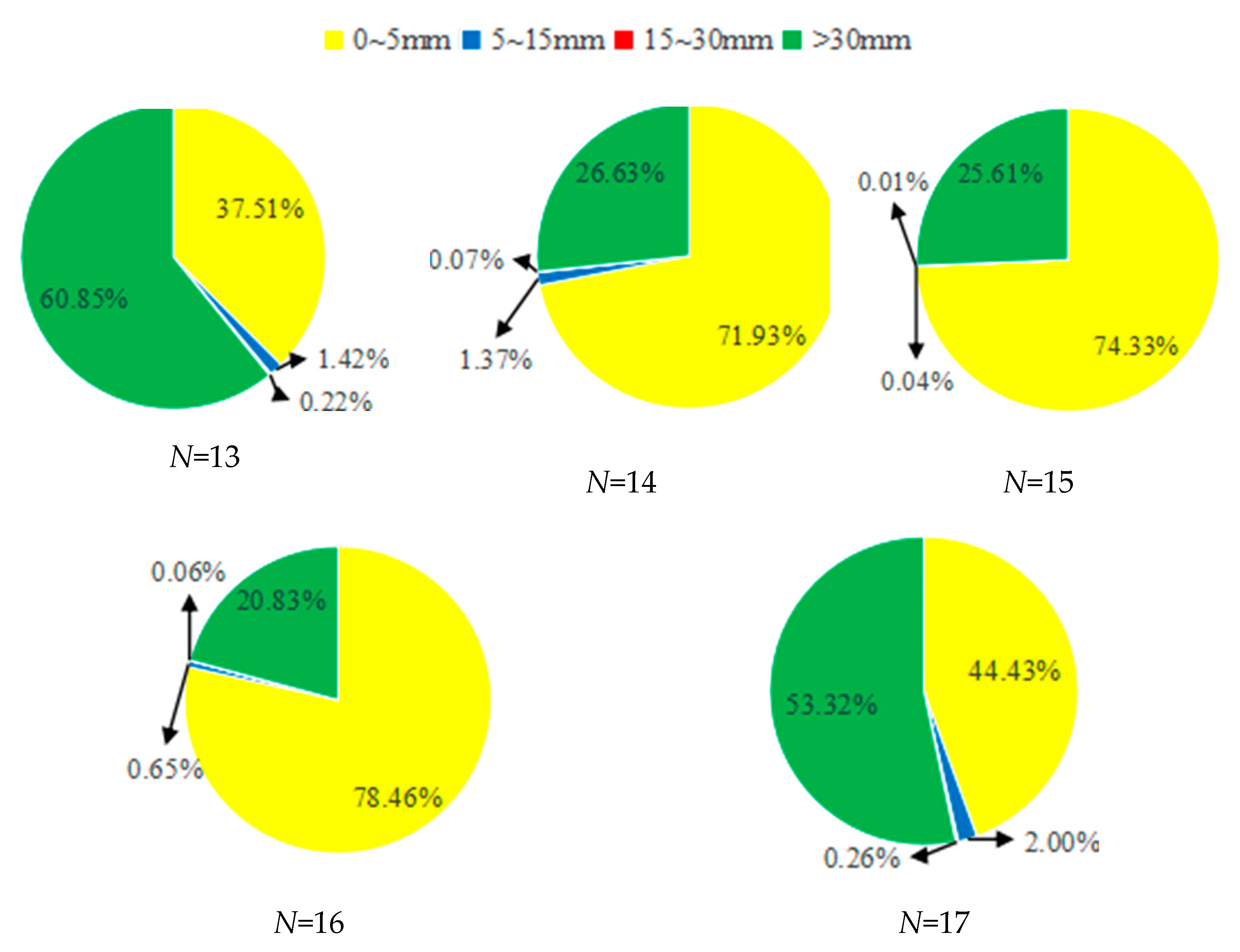
To further reveal the spatial distribution of energy loss inside the runner and quantify the entropy production contribution of different flow regions, the runner passage was divided, with the runner rotation center as the reference, into four regions: the near-wall region (0–5 mm), the secondary near-wall region (5–15 mm), the intermediate-flow region (15–30 mm), and the core-flow region (>30 mm). The threshold distances for the runner region were selected following the same approach as for the guide vane region, based on the local boundary-layer characteristics and near-wall grid resolution. A similar sensitivity analysis confirmed that the conclusions are insensitive to the exact threshold values. On this basis, volume integration of the entropy production rate was performed for each region, and the results are shown in Figure 15.

As expected for turbulent flows in hydraulic turbines, the entropy production distribution in the runner shows evident spatial stratification, with the near-wall region dominating the entropy production. This confirms the physical consistency of our simulations. The more meaningful comparison among the schemes is presented below, where the differences in regional entropy production distribution are analyzed across the five blade-number configurations.

From the comparison among schemes, the near-wall proportion of the N = 13 scheme is relatively low, while the loss proportions in the intermediate-flow and wall-distant regions are relatively high, indicating stronger flow diffusion and a more dispersed energy-loss distribution when the blade number is small. In the N = 14 scheme, the near-wall proportion increases and the flow gradually becomes more controlled. In the N = 15 scheme, the near-wall proportion is moderate and the distribution among regions is the most balanced. In particular, its core-flow proportion is the lowest, indicating a more stable flow structure and the weakest concentration of loss. In the N = 16 and N = 17 schemes, the near-wall proportion further increases, showing that increasing blade density strengthens wall-friction effects and causes energy loss to concentrate more near the wall.

Although all schemes are dominated by near-wall entropy production, the N = 15 scheme performs best in terms of spatial-distribution uniformity and coordinated multi-region loss allocation. It can effectively suppress local entropy production concentration, further verifying its superior runner flow quality and hydraulic performance.

Although all schemes are dominated by near-wall entropy production, the N = 15 scheme performs best in terms of spatial-distribution uniformity and coordinated multi-region loss allocation. A balanced entropy production distribution is advantageous because concentrated entropy-production regions are often associated with local shear layers, vortex structures, or flow separations that can induce pressure pulsations, vibrations, and fatigue loads. By effectively suppressing local entropy production concentration, the N = 15 scheme not only achieves low overall losses but also ensures a more organized flow and improved operational stability, particularly under off-design conditions. This further verifies its superior runner flow quality and hydraulic performance.

4.2.3. Flow-Field Comparison in the Draft Tube Region

• Velocity Streamline Comparison;

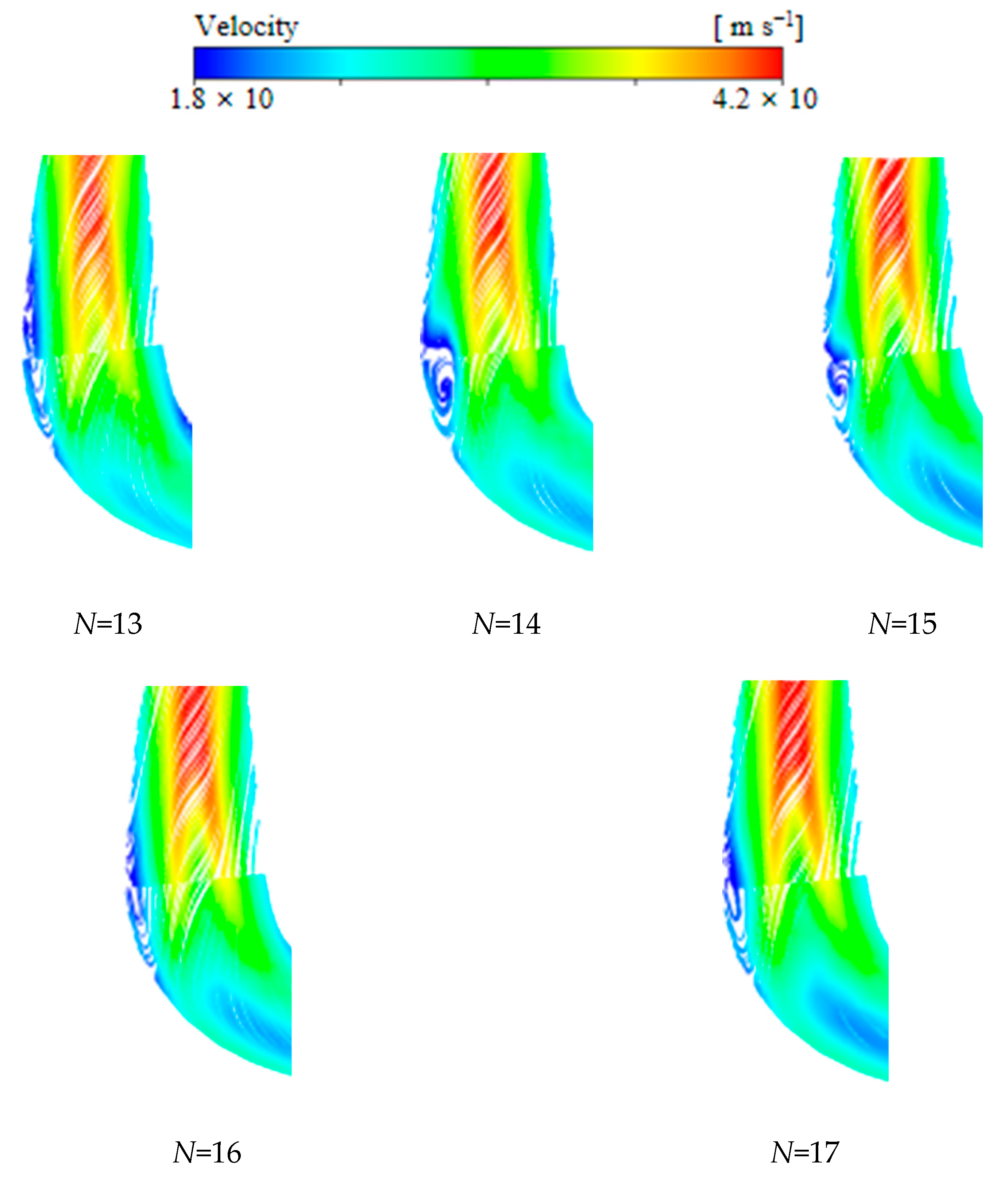
Figure 16 shows the velocity streamline distributions in the draft tube region under OC5 for different long–short blade schemes. It can be seen that a certain swirl structure exists at the draft tube inlet in all schemes, because the flow carries residual rotational kinetic energy after passing through the runner. In the N = 13 and N = 14 schemes, the swirl is relatively pronounced, local streamline curling occurs, and flow-field uniformity is poor. In the N = 15 scheme, the streamlines are the most uniform, the transition through the elbow region is smooth, and the swirl intensity is weak. No obvious backflow or streamline clustering is observed, indicating good flow recovery capability. In the N = 16 and N = 17 schemes, although the streamlines are generally continuous, local streamline clustering and non-uniform velocity distribution still exist.

Comprehensive comparison shows that the N = 15 scheme produces the smoothest flow inside the draft tube, with the best streamline uniformity and continuity. This is beneficial for weakening the development of swirl and secondary flow and for improving the energy recovery capability of the draft tube.

2.

Pressure distribution;

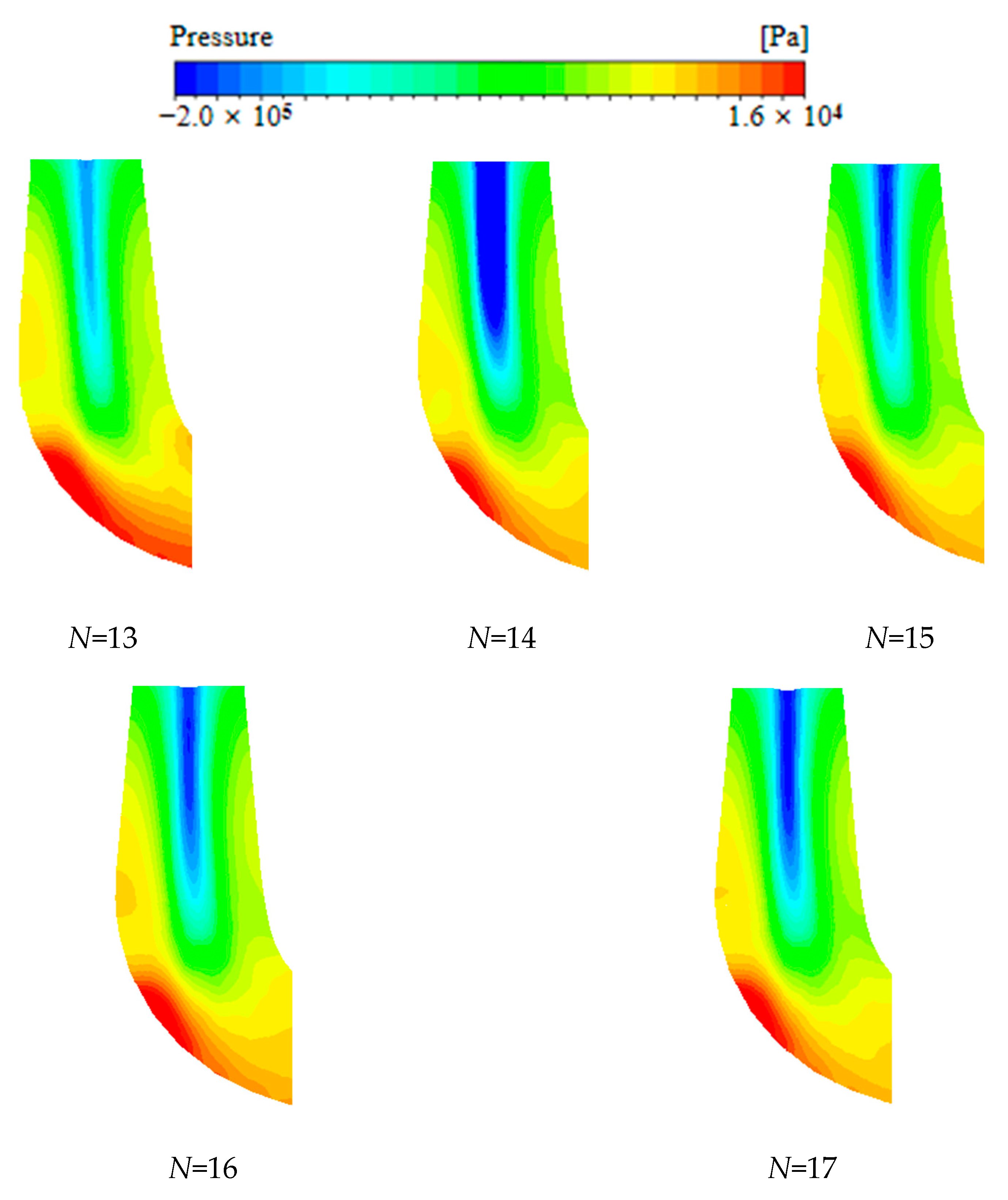
Figure 17 presents the static pressure contours in the draft tube region under OC5 for different long–short blade schemes. In all schemes, static pressure inside the draft tube gradually recovers from the inlet toward the downstream direction. For the N = 13 and N = 14 schemes, the low-pressure region is more extensive, indicating relatively weak pressure recovery capability. The N = 15 scheme shows relatively uniform pressure distribution, a narrowed low-pressure region and smooth pressure transition. The N = 16 and N = 17 schemes possess generally stable pressure distribution, with minor local spatial unevenness.

Comprehensive comparison indicates that the N = 15 scheme achieves better pressure uniformity and pressure recovery in the draft tube. Combined with the velocity streamline analysis, this scheme contributes to improved flow uniformity and energy recovery capability.

3.

Entropy production distribution.

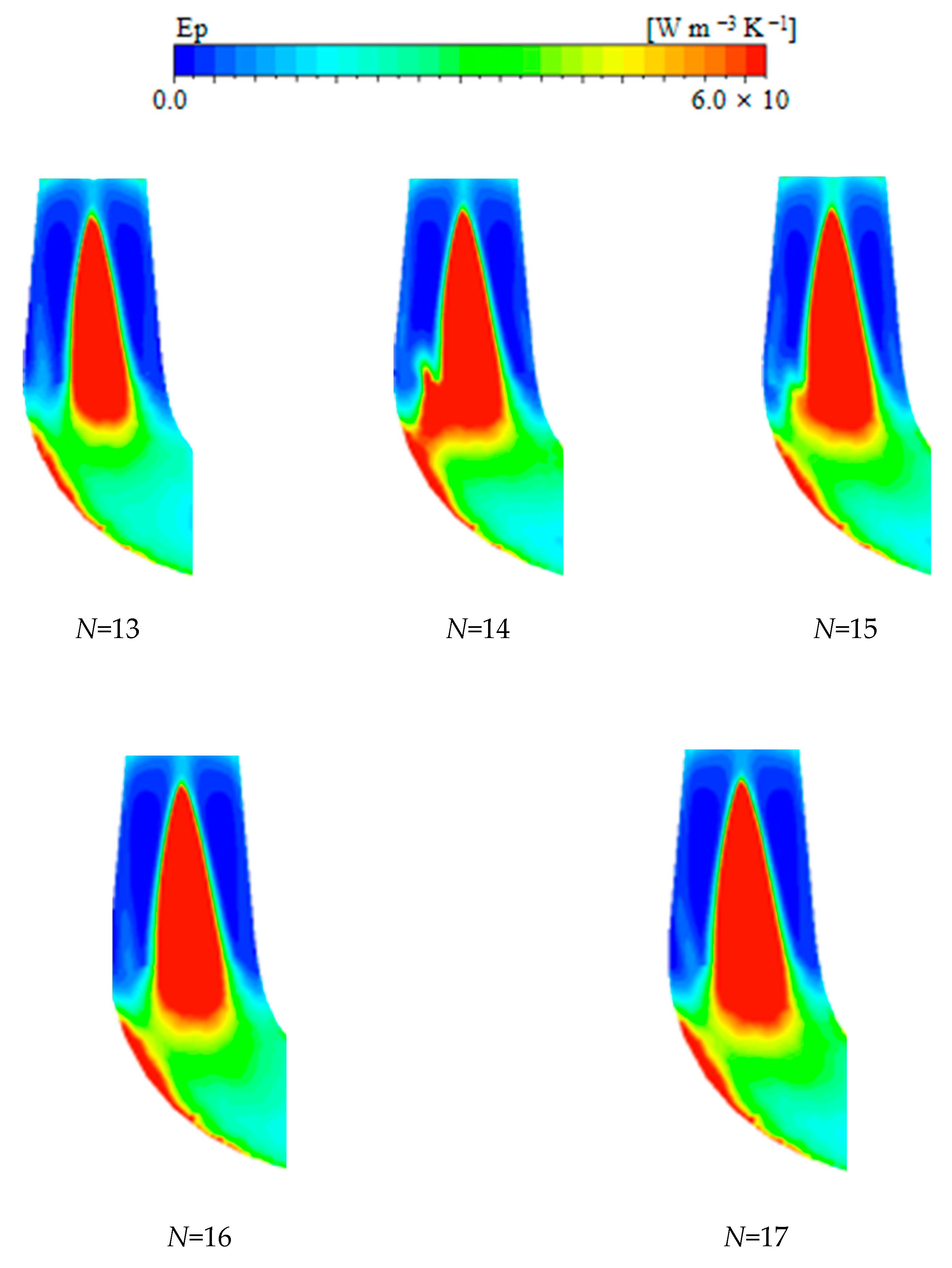
Figure 18 shows the entropy production rate contours in the draft tube region under OC5 for different long–short blade schemes. The high-entropy-production regions of all schemes are mainly concentrated near the draft tube inlet and the elbow transition section. This concentration results from the combined effects of residual swirl at the runner outlet, velocity gradients, and changes in flow direction.

To quantify the extent of high-entropy-production regions in the draft tube, the volume of regions with entropy production rates above 1364.5 W m⁻³ K⁻¹ (50% of the maximum value in the N = 15 scheme) was calculated for each scheme. Normalized by the total draft tube volume (3.52247 m³, identical for all schemes), the high-entropy-production volumes are: N = 13: 42.4%, N = 14: 45.8%, N = 15: 39.7%, N = 16: 46.8%, and N = 17: 49.8%. The results confirm that the N = 15 scheme has the smallest normalized high-entropy-production volume, quantitatively demonstrating its superior ability to suppress local energy dissipation.

In the N = 13 and N = 14 schemes, the high-entropy-production region is relatively large, and obvious local entropy production accumulation exists, indicating serious flow separation and turbulent dissipation inside the draft tube. In the N = 15 scheme, the high-entropy-production area is the smallest and is mainly concentrated near the draft tube inlet; entropy production in the elbow and diffuser sections is relatively uniform. This indicates that the scheme can effectively weaken residual swirl and reduce energy loss inside the draft tube.

Compared with the N = 15 scheme, the high-entropy-production regions of the N = 16 and N = 17 schemes expand. In the N = 16 scheme, a high-entropy-production band on the outer side of the elbow is relatively evident. The N = 17 scheme shows some improvement, but local entropy production concentration still exists, reflecting a certain degree of energy dissipation in the draft tube.

Overall, the N = 15 scheme has the smallest and most uniform high-entropy-production region and the lowest energy loss in the draft tube. Together with the preceding analyses of velocity streamlines and pressure distribution, these results show that this scheme has the best flow recovery capacity and energy recovery effect, further demonstrating its superior comprehensive hydraulic performance.

5. Discussion

The results demonstrate that blade number exerts a significant but non-monotonic influence on Francis turbine performance. The N = 15 scheme achieves the highest overall efficiency under rated and high-flow conditions, whereas the N = 16 scheme exhibits the lowest efficiency despite having more blades than N = 15. This non-monotonic behavior reflects a trade-off between two competing mechanisms: increasing blade number improves flow guidance and suppresses secondary flows but also increases wetted surface area and friction losses. The optimal blade number, which occurs at N = 15 in this study, represents the best balance between these opposing effects.

The anomalously low efficiency of the N = 16 scheme suggests that blade number alone does not determine performance. The specific interaction between blade count and the upstream flow field—including incidence angle and velocity distribution from the guide vanes—likely plays a critical role, as evidenced by the disproportionately high losses in the guide vane and draft tube regions for this configuration (Figure 7). This observation aligns with previous findings that blade number affects not only runner performance but also downstream flow characteristics.

The entropy production analysis reveals that near-wall losses dominate in both the guide vanes (76–77%) and the runner, consistent with the theoretical framework of Kock and Herwig. The N = 15 scheme achieves the most balanced entropy production distribution between near-wall and far-wall regions, indicating well-organized flow with neither excessive wall friction nor pronounced flow separation.

In the draft tube, the N = 15 scheme exhibits the weakest inlet swirl and the smallest high-entropy-production region, confirming that improved runner outflow conditions enhance downstream pressure recovery.

The practical implications of these findings extend to the operation and maintenance strategies of rural small hydropower stations. The N = 15 configuration, by achieving the most uniform flow distribution and the lowest non-runner losses, is expected to exhibit not only higher efficiency but also improved operational stability. This is particularly relevant for rural power grids that increasingly integrate distributed photovoltaics and wind power, where small hydropower units are frequently required to operate under variable-load conditions for peak shaving and load following. The balanced performance of the N = 15 scheme across the full flow range (Figure 5 and Figure 6) makes it well-suited for such flexible operation. Furthermore, the reduction in entropy production and weakened draft tube swirl observed in the N = 15 scheme may contribute to lower vibration and fatigue loads, potentially extending the maintenance intervals and service life of the turbine—a crucial economic factor for off-grid rural communities where maintenance resources are limited. Therefore, the findings provide direct engineering guidance for both runner retrofitting and new unit selection in rural electrification projects.

A closer examination of the runner efficiency versus overall efficiency reveals an interesting trade-off mechanism. Although the N = 17 (purple) scheme achieves superior runner efficiency due to its denser blade arrangement, which provides better flow guidance and suppresses secondary flow losses inside the runner passages (Figure 6), this advantage in the runner does not translate into the highest overall unit efficiency. The primary reason is that the denser blade arrangement in the N = 17 scheme alters the outflow conditions at the runner outlet, resulting in a stronger residual swirl entering the draft tube. This increased swirl intensity causes additional hydraulic losses in the draft tube, as evidenced by the larger high-entropy-production regions observed in Figure 18 for the N = 17 scheme compared with the N = 15 scheme. In addition, the increased blade surface area in the N = 17 scheme leads to higher friction losses at the runner inlet and outlet regions, which partially offsets the gains from improved flow guidance. By contrast, the N = 15 (green) scheme achieves a more favorable balance: its blade density is sufficient to maintain good flow guidance and suppress secondary flows, while not being so dense as to cause excessive friction losses or adverse draft tube flow conditions. As a result, the N = 15 scheme delivers the best overall efficiency across the full operating range, even though its runner efficiency alone is slightly lower than that of the N = 17 scheme. This trade-off between runner performance and downstream flow recovery is a key factor governing the non-monotonic variation of hydraulic performance with blade number observed in this study.

Several limitations should be acknowledged. The study is based solely on steady-state numerical simulations without experimental validation. Acknowledging the computational nature of this study, a key limitation is the absence of experimental validation. This is primarily due to the unavailability of a physical model test rig for the prototype turbine, as well as constraints related to instrumentation and measurement access in rural small hydropower settings. Nevertheless, several measures were taken to enhance confidence in the CFD results: (1) a rigorous grid independence verification based on the GCI method [26] confirmed that the numerical uncertainty remains below 0.12%; (2) the SST-DES model employed in this study has been widely validated in previous hydraulic turbine studies [12,16,23], demonstrating good predictive capability for both time-averaged and unsteady flow features; and (3) the efficiency trends and loss distributions obtained are physically consistent with established theoretical principles, such as the trade-off between flow guidance and friction losses as blade number varies. Future work should include experimental model testing or field measurements to further validate the numerical findings.

6. Conclusions

This study investigated a Francis turbine with long and short blades. CFD simulations were used to analyze the effects of five blade-number configurations (N = 13–17) on hydraulic efficiency, flow field, and entropy production characteristics. The main conclusions are as follows:

(1) Blade number exerts a significant but non-monotonic influence on turbine performance. Increasing blade number improves flow confinement under low-load conditions, but overly dense blades increase friction loss in the high-flow range. The N = 15 scheme provides the best overall performance across the full operating range.

(2) The N = 15 scheme provides the best balance among efficiency, loss allocation, and flow matching. Its overall efficiency remains high across the full-flow range, while non-runner losses (guide vanes and draft tube) are minimized. This demonstrates optimal system matching and full-condition adaptability.

(3) Flow-field and entropy production analyses confirm that the N = 15 scheme exhibits the most uniform velocity streamlines, the mildest pressure gradients, and the smallest high-entropy-production regions across all components. Its near-wall and far-wall entropy production distributions are the most balanced, indicating well-organized flow with neither excessive wall friction nor pronounced flow separation.

(4) It should be noted that the optimal blade number of N = 15 identified in this study is specific to the runner geometry, design head, and operating conditions examined. Variations in turbine specific speed, blade profile, or meridional channel shape may shift the optimal blade number. Nevertheless, the results suggest that the N = 15 scheme offers a favorable balance between rated-point performance and off-design stability, making it a suitable candidate for engineering applications.

References

1. Mukherjee, A.; Khullar, S.; Ud Din, M.Z.; Pant, C.S.; Kumar, A. A comparative analysis of CFD methodologies to predict the performance of Francis turbine. IOP Conf. Ser. Earth Environ. Sci. 2024, 1411, 012009. [Google Scholar] [CrossRef]
2. Zhu, W.; Gao, Z.; Tang, Y.; Zhang, J.; Lu, L. Adaptability of turbulence models to predict the performance and blade surface pressure prediction of a Francis turbine. Eng. Comput. 2016, 33, 238–251. [Google Scholar] [CrossRef]
3. Umar, B.M.; Huang, X.X. Numerical investigation of performance and flow characteristics of Francis turbine in part load condition. J. Phys. Conf. Ser. 2024, 2752, 012006. [Google Scholar] [CrossRef]
4. Tiwari, G.; Kumar, J.; Shukla, S.N.; Prasad, V.; Patel, V.K. Multi-fidelity CFD approach for hydrodynamic performance analysis of a prototype Francis turbine—A comparative study. In Fluid Mechanics and Fluid Power; Lecture Notes in Mechanical Engineering; Bhattacharyya, S., Benim, A.C., Eds.; Springer: Singapore, 2023; Volume 2, pp. 123–128. [Google Scholar] [CrossRef]
5. Tiwari, G.; Kumar, J.; Prasad, V.; Patel, V.K. Multi-fidelity CFD for obtaining the runner blade profile parameters of a Francis turbine for optimum hydrodynamic performance. Ocean Eng. 2024, 312, 117994. [Google Scholar] [CrossRef]
6. Zhang, X.; Nie, C.; Luo, Z. The influence of structure optimization on vortex suppression and energy dissipation in the draft tube of Francis turbine. Processes 2024, 12, 2249. [Google Scholar] [CrossRef]
7. Wang, H.; Zhou, D.; Guo, J.; Xu, L. Analysis of hydraulic losses in vortex rope inside the draft tube of Francis pump-turbine based on entropy production theory. Machines 2023, 11, 965. [Google Scholar] [CrossRef]
8. Favrel, A.; Irie, T.; Ishii, Y.; Lee, N.J.; Miyagawa, K. Experimental and numerical validation of a Francis turbine draft tube designed for mitigation of pressure fluctuations. IOP Conf. Ser. Earth Environ. Sci. 2022, 1079, 012017. [Google Scholar] [CrossRef]
9. Wang, H.; Zhou, D.; Yu, A.; Guo, J. Analysis of cavitation-induced unsteady flow conditions in Francis turbines under high-load conditions. Processes 2024, 12, 72. [Google Scholar] [CrossRef]
10. Li, P.; Lu, J.; Tao, R.; Xiao, R.; Ji, B.; Wang, F. Energy distribution and chaotic pressure analysis of vortex ropes in Francis-99. Eng. Appl. Comput. Fluid Mech. 2024, 18, 2310609. [Google Scholar] [CrossRef]
11. Shahzer, M.A.; Cho, Y.; Shamsuddeen, M.M.; Kim, J.H. Investigation of cavitating vortex rope instabilities and its suppression inside a Francis turbine model with Thoma number variation. Phys. Fluids 2023, 35, 033310. [Google Scholar] [CrossRef]
12. Wang, W.; Yu, Z.; Yan, Y.; Wei, X. Numerical investigation on vortex characteristics in a low-head Francis turbine operating of adjustable-speed at part load conditions. Energy 2024, 302, 131800. [Google Scholar] [CrossRef]
13. Trivedi, C.; Cervantes, M.J.; Gandhi, B.K.; Dahlhaug, O.G. Transient Pressure Measurements on a High Head Model Francis Turbine During Emergency Shutdown, Total Load Rejection, and Runaway. J. Fluids Eng. 2014, 136, 121107. [Google Scholar] [CrossRef]
14. Favrel, A.; Müller, A.; Landry, C.; Yamamoto, K.; Avellan, F. Study of the vortex-induced pressure excitation source in a Francis turbine draft tube by particle image velocimetry. Exp. Fluids 2015, 56, 215. [Google Scholar] [CrossRef]
15. Masoodi, F.; Goyal, R. Simulation and validation of a Francis turbine load rejection procedure using OpenFOAM CFD code. IOP Conf. Ser. Earth Environ. Sci. 2024, 1411, 012064. [Google Scholar] [CrossRef]
16. Ramdani, S.; Shingai, K.; Kobayashi, K.; Sato, K.; Tamura, Y. Large eddy simulation analysis of Francis turbine: A comparison with experimental data and investigation of vortex rope dynamics in the draft tube. IOP Conf. Ser. Earth Environ. Sci. 2024, 1411, 012055. [Google Scholar] [CrossRef]
17. Wen, Q.; Guo, P.; Wang, Z.; Sun, L. Numerical study on flow characteristics of Francis turbines based on weak compressibility. Mech. Electr. Tech. Hydropower Stn. 2024, 47, 9–14. [Google Scholar]
18. Lu, J.; Su, C.; Tao, R. Influence of runner blade number on hydraulic performance and flow control in draft tube of Francis turbine. Adv. Mech. Eng. 2024, 16, 1–20. [Google Scholar] [CrossRef]
19. Kumar, P.; Singal, S.K.; Gohil, P.P. Numerical analysis of cavitation characteristics of Francis turbine at different runner blade numbers. IOP Conf. Ser. Earth Environ. Sci. 2024, 1411, 012062. [Google Scholar] [CrossRef]
20. Dahal, D.R.; Trivedi, C. Effect of runner blade numbers on inter-blade vortices of Francis turbine under best efficiency loading. IOP Conf. Ser. Earth Environ. Sci. 2025, 1483, 012025. [Google Scholar] [CrossRef]
21. Sun, L.; Guo, P.; Luo, X. Numerical investigation on inter-blade cavitation vortex in a Francis turbine. Renew. Energy 2020, 158, 64–74. [Google Scholar] [CrossRef]
22. Jia, Y.; Wei, X.; Wang, Q.; Cui, J.; Li, F. Experimental study of the effect of splitter blades on the performance characteristics of Francis turbines. Energies 2019, 12, 1676. [Google Scholar] [CrossRef]
23. Song, Y.; Guo, P.; Sun, L.; Zhou, H.; Luo, X. Multidisciplinary design optimization on the splitter blade of high head Francis turbine. IOP Conf. Ser. Earth Environ. Sci. 2018, 163, 012032. [Google Scholar] [CrossRef]
24. Chen, H.; Lu, Y.; Liu, K.; Zhang, Z.; Li, H.; Huang, X.; Zhao, W.; Wang, Z. Study on the Internal Flow Characteristics of Long and Short Blade Runners of a 1000 MW Francis Turbine under Different Opening Conditions. Processes 2023, 11, 1796. [Google Scholar] [CrossRef]
25. Versteeg, H.K.; Malalasekera, W. An Introduction to Computational Fluid Dynamics: The Finite Volume Method, 2nd ed.; Pearson Education: Harlow, UK, 2007; pp. 1–45. [Google Scholar]
26. Kock, F.; Herwig, H. Local entropy production in turbulent shear flows: A high-Reynolds-number model with wall functions. Int. J. Heat Mass Transf. 2004, 47, 2205–2215. [Google Scholar] [CrossRef]
27. Celik, I.B.; Ghia, U.; Roache, P.J.; Freitas, C.J. Procedure for estimation and reporting of uncertainty due to discretization in CFD applications. J. Fluids Eng. 2008, 130, 078001. [Google Scholar] [CrossRef]
Figure 1. Three-dimensional geometric assembly model of the full-passage turbine.
Water 18 01950 g001
Figure 2. Geometric model of the runner with long and short blades.
Water 18 01950 g002
Figure 3. Full-passage assembly of the meshed turbine.
Water 18 01950 g003
Figure 4. Mesh independence verification results.
Water 18 01950 g004
Figure 5. Overall hydraulic efficiency versus flow rate for different long–short blade schemes.
Water 18 01950 g005
Figure 6. Runner hydraulic efficiency versus flow rate for different long–short blade schemes.
Water 18 01950 g006
Figure 7. (a) Energy-loss proportion of each component under OC5 for different long–short blade schemes. (b) Magnified view of energy losses in the non-runner components (guide vanes, draft tube, and others) under OC5 for different long–short blade schemes.
Water 18 01950 g007aWater 18 01950 g007b
Figure 8. Comparison of guide vane velocity streamlines under OC5 for different long–short blade schemes.
Water 18 01950 g008
Figure 9. Guide vane pressure distribution under OC5 condition for different long–short blade schemes.
Water 18 01950 g009
Figure 10. Entropy production-rate contours in the guide vane region under OC5 for different long–short blade configurations.
Water 18 01950 g010aWater 18 01950 g010b
Figure 11. (a) Schematic illustration of the guide vane showing the division between the near-wall region (red, within 5 mm from the wall) and the far-wall region (blue, beyond 5 mm). (b) Comparison of entropy production in near-wall and far-wall regions of the guide vane under OC5 for different long–short blade schemes.
Water 18 01950 g011
Figure 12. Velocity streamline distributions in the runner region under OC5 for different schemes.
Water 18 01950 g012
Figure 13. Pressure contours on the long and short runner blades under OC5 for different schemes.
Water 18 01950 g013
Figure 14. Entropy production contours in the runner region under OC5 for different schemes.
Water 18 01950 g014aWater 18 01950 g014b
Figure 15. Regional entropy-production-rate proportions in the runner region under OC5 for different schemes.
Water 18 01950 g015
Figure 16. Comparison of draft tube velocity streamlines under OC5 for different long–short blade schemes.
Water 18 01950 g016
Figure 17. Draft tube pressure distribution under OC5 for different long–short blade schemes.
Water 18 01950 g017
Figure 18. Entropy production distribution in the draft tube under OC5 for different long–short blade schemes.
Water 18 01950 g018