Deep Learning for Remote Sensing-Based Surface Soil Moisture Monitoring and Prediction: A Review

Abstract

Surface soil moisture (SM) is the keystone variable of terrestrial ecohydrology. Yet, the rapid diversification and development of deep learning architectures for satellite SM estimation have outpaced practitioners’ capacity to select among them. This review synthesizes 37 deep learning studies from the SMAP era (2015–2026) across five architecture families (MLP and physics-informed neural networks [MLP/PINN], long short-term memory [LSTM] and gated recurrent unit [GRU] networks, convolutional neural networks [CNN], convolutional LSTM and graph neural networks [GNN], and Transformer-based models) to establish an architecture–task-matching framework that links each family to its dominant estimation niche. The analysis reveals consistent specializations: MLP/PINN models achieve competitive surface SM retrieval from satellite inputs; recurrent networks extend SMAP temporally (RMSE ≤ 0.035  ${\mathrm{m}}^3\hspace{0.17em}{\mathrm{m}}^{-3}$); CNN disaggregates SMAP to 1 km (reported unbiased root-mean-square error (ubRMSE) approaching 0.04  ${\mathrm{m}}^3\hspace{0.17em}{\mathrm{m}}^{-3}$); ConvLSTM and GNN address spatiotemporal gap-filling (low reported ubRMSE 0.022  ${\mathrm{m}}^3\hspace{0.17em}{\mathrm{m}}^{-3}$); and Transformers enable global multi-source fusion and decadal climate-scenario projection. Across all families, four physics-DL integration modes (hard architectural constraints, soft loss-function penalties, physics-as-input feature engineering, and physics-ML hybrid output fusion) consistently yield RMSE reductions of 8–50% relative to data-driven baselines. These findings provide a practitioner-oriented framework that is applicable to ecohydrological monitoring of plant water stress, agricultural drought, early flood warnings, and land–atmosphere coupling.

1. Introduction

Across spatial scales from field plots to continental landmasses, soil moisture (SM) is the keystone variable of terrestrial ecohydrology, governing precipitation partitioning into infiltration and runoff, sustaining plant transpiration and vegetation water availability, regulating land surface energy fluxes through evaporative cooling, and coupling the water, carbon, and energy cycles [1]. Drought onset, vegetation productivity, groundwater recharge, and the intensity of land–atmosphere moisture recycling are each strongly conditioned on the surface SM state; spatially explicit, temporally continuous SM information is therefore indispensable for ecosystem water-stress monitoring, agricultural early warnings, and climate impact assessments [2]. At the ecosystem scale, SM governs evapotranspiration and the partitioning of net primary productivity between carbon uptake and water loss, sustains water-mediated biogeochemical cycles in riparian and wetland systems, and determines the resilience of aquatic and terrestrial ecosystems to drought, flood, and land-use changes—three dimensions central to the ecohydrological monitoring and prediction goals.

Satellite remote sensing has delivered global SM observations since the late 1970s [3]. Still, the launch of the NASA Soil Moisture Active Passive (SMAP) mission in 2015 marked a change in steps: the SMAP mission provided dedicated L-band passive radiometry with a stated accuracy target of ubRMSE ≤ 0.04  ${\mathrm{m}}^3\hspace{0.17em}{\mathrm{m}}^{-3}$ [1] and a near-daily global revisit at 36 km. The concurrent maturation of Sentinel-1 synthetic aperture radar (SAR), which has provided 10 m dual-polarization C-band observations with a 6-day revisit since 2014, has offered the first globally systematic high-resolution active microwave SM signal [4]. Yet, two fundamental limitations persist across all current satellite SM products: (i) the spatial resolution is too coarse (9–36 km) for field- and watershed-scale applications; and (ii) there are temporal gaps between revisit schedules and cloud or frozen-soil screening that interrupt the time series at critical phenological transitions.

The SMAP era coincided with a deep learning (DL) revolution in geoscience that fundamentally changed how satellite SM information is extracted and extended. Fang et al. [5] demonstrated what appears to be the first application of long short-term memory (LSTM) networks to continental-scale SMAP SM temporal gap-filling by predicting SMAP products from atmospheric forcing with an RMSE < 0.035  ${\mathrm{m}}^3\hspace{0.17em}{\mathrm{m}}^{-3}$ across more than 75% of CONUS—a result that no conventional empirical method has achieved at continental scale. Since then, DL architectures for SM estimation have progressed from feedforward artificial neural networks (ANNs) for multi-source satellite SM retrieval, through convolutional networks for spatial downscaling and ConvLSTM architectures for spatio-temporal gap-filling, to graph neural networks for sensor-network prediction and Transformer-based fusion for global SM reconstruction and climate projection. In parallel, physics-guided DL has emerged as a particularly powerful paradigm: by embedding governing equations directly into training objectives, including the I²EM scattering model and water cloud model for surface SM retrieval from SAR observations, these methods generally improve accuracy and physical consistency while demonstrating robustness to data scarcity in controlled experiments.

Several comprehensive reviews have addressed DL and remote sensing for SM in recent years, but none have provided the architecture-progressive, physics-integration-centered perspective this field now requires. Montzka et al. [6] provided the most comprehensive structured overview of AI methods for satellite SM retrieval, organized by the sensor type (passive, active, and SAR) rather than by the DL architecture, and therefore did not trace the progressive capability trajectory from MLP to Transformer that characterizes the SMAP era. Wang et al. [7] rigorously benchmarked ten DL architectures for SM prediction at 30 in situ point sites without addressing satellite-based SM products. Rahmati et al. [4] reviewed the full spectrum of Sentinel-1 SM retrieval methods, from physics-based inversion to AI, as a sensor-specific compendium of lessons learned rather than as a DL architecture survey. Lamichhane et al. [3] synthesized 144 ML studies from 2010 to 2024, with a focus on classical algorithms (random forest, 47%; SVR, 27%; ANN, 19%) rather than the DL families that now dominate state-of-the-art SM estimation. Ramaiah et al. [8] surveyed AI frameworks for SM estimation from remote sensing satellite imagery, emphasizing challenges and opportunities rather than architecture-specific performance. No existing review organizes SMAP-era DL for SM by architecture family, from MLP/PINN through LSTM/GRU, CNN, and ConvLSTM/GNN to Transformers, while treating physics-DL integration as a unifying analytical thread and connecting the resulting capability map to ecohydrological applications.

This review addresses that gap by providing the first architecture-progressive synthesis of deep learning for remote sensing-based surface SM monitoring and prediction in the SMAP era (2015 onward). The review makes four specific contributions. First, it organizes the DL SM literature by dominant architecture family, demonstrating how each family occupies a distinct task niche (satellite SM retrieval for the MLP/PINN family; spatial downscaling for CNN; temporal prediction and spatiotemporal gap-filling for recurrent and ConvLSTM/GNN architectures; and multi-source fusion for Transformers) and establishing a practitioner-oriented architecture–task-matching framework. Second, it identifies four modes of physics-DL integration (hard architectural constraints, soft loss-function penalties, physics-as-input feature engineering, and physics-ML hybrid fusion output) and traces their quantified benefits across all five architecture families. Third, it provides a contextual guide to the evaluation metrics and representative studies (

Table 1. Evaluation metrics for deep learning SM models.

Metric	Equation	Description
ubRMSE	$\mathrm{ubRMSE}=\sqrt{{\mathrm{RMSE}}^2-{\mathrm{Bias}}^2}$	Unbiased Root-Mean-Square Error $({\mathrm{m}}^3\hspace{0.17em}{\mathrm{m}}^{-3}$).Removes systematic bias to isolate random retrieval errors. It is the primary SMAP mission benchmark (target ≤ 0.04 ${\mathrm{m}}^3\hspace{0.17em}{\mathrm{m}}^{-3}$).
RMSE	$\mathrm{RMSE}=\sqrt{{\displaystyle \frac{1}{n}}{\displaystyle \sum _{i=1}^n}{\left({\widehat{p}}_i-p_i\right)}^2}$	Root-Mean-Square Error (${\mathrm{m}}^3\hspace{0.17em}{\mathrm{m}}^{-3}$). Measures total-error magnitude (combining both random and systematic components). Heavily penalized by large deviations.
Bias	$\mathrm{Bias}={\displaystyle \frac{1}{n}}{\displaystyle \sum _{i=1}^n}\left({\widehat{p}}_i-p_i\right)$	Mean Systematic Offset (${\mathrm{m}}^3\hspace{0.17em}{\mathrm{m}}^{-3}$). Indicates overestimation (positive) or underestimation (negative). Reported alongside ubRMSE to separate bias from random errors.
R	$R={\displaystyle \frac{{\displaystyle {\sum }_{i=1}^n}\left({\widehat{p}}_i-\overline{\widehat{p}}\right)\left(p_i-\overline{p}\right)}{\sqrt{{\displaystyle {\sum }_{i=1}^n}{\left({\widehat{p}}_i-\overline{\widehat{p}}\right)}^2\cdot {\displaystyle {\sum }_{i=1}^n}{\left(p_i-\overline{p}\right)}^2}}}$	Pearson linear correlation coefficient. Measures temporal pattern agreement independently of mean bias. Widely reported in conjunction with ubRMSE for SM satellite validation.
R2	$R^2={\left({\displaystyle \frac{{\displaystyle \sum _{i=1}^n({\widehat{p}}_i-\overline{\widehat{p}})}(p_i-\overline{p})}{\sqrt{{\displaystyle {\displaystyle \sum _{i=1}^n}{({\widehat{p}}_i-\overline{\widehat{p}})}^2}\cdot {\displaystyle {\displaystyle \sum _{i=1}^n}{(p_i-\overline{p})}^2}}}}\right)}^2$	Coefficient of determination. Proportion of SM variance explained by the model. Commonly reported in single-site studies and spatial downscaling evaluations.

and Table 2), allowing readers to interpret values alongside the task type, spatial scale, region, validation settings, and metric definitions rather than as a cross-study ranking. Fourth, it connects the reviewed DL capabilities to ecohydrological monitoring needs (plant water stress, drought monitoring, land–atmosphere coupling, and early flood warning) and identifies two frontier research directions that are aligned with remote sensing for ecohydrological monitoring and prediction.

The remainder of this review is organized as follows. Section 2 describes the review methodology and introduces the five DL architecture families (MLP/PINN, LSTM/GRU, CNN, ConvLSTM/GNN, and Transformer), together with the primary satellite datasets and evaluation metrics (Table 1) used in SMAP-era SM research. Section 3 surveys DL applications to SM estimation by dominant architecture. Section 4 synthesizes the architecture–task boundaries, the physics-DL integration trajectory, persistent performance challenges, and ecohydrological implications. Section 5 presents the main conclusions.

2. Materials and Methods

To improve transparency and reproducibility, we explicitly defined the review scope as remote sensing-based DL studies on surface SM published during the SMAP era. We searched the Web of Science database through our university’s institutional subscription and supplemented the search with backward reference screening. The search strategy combined the following soil moisture terms (“soil moisture”, “surface soil moisture”, “SM”, and “SMAP”), remote sensing terms (“remote sensing”, “satellite”, “microwave”, “SAR”, “Sentinel-1”, “AMSR-E”, “AMSR2”, “ASCAT”, and “ESA CCI”), and DL architecture terms (“deep learning”, “neural network”, “MLP”, “PINN”, “LSTM”, “GRU”, “CNN”, “ConvLSTM”, “GNN”, and “Transformer”). We retained application studies that used satellite or satellite-assisted inputs to estimate, predict, downscale, reconstruct, or gap-fill surface SM. We excluded review articles from the core application-study sample, methodological papers without a soil moisture application, studies focused on unrelated land surface variables, duplicate reports of the same work, and papers whose primary target was root-zone or deep soil moisture rather than surface SM. Relevant reviews were cited separately for background and positioning but were not counted among the 37 DL application studies. Screening proceeded from title and abstract to full text, and the final core set comprised 37 DL application studies.

A small number of adjacent subsurface, root-zone, or irregular-network studies were retained only as methodological exemplars when they helped clarify architecture boundaries, transfer learning, uncertainty analysis, or physics-DL integration. These exemplars are explicitly treated as boundary cases rather than as part of the core 37-study sample.

SM remote sensing has evolved from single-sensor empirical retrieval algorithms to deep learning architectures that are capable of jointly integrating multi-source inputs (passive microwave radiances, active SAR backscatter, optical indices, and reanalysis fields). The transition mirrors a broader deep learning surge in geoscience: early artificial neural network approaches that encoded simple radiance-to-SM mappings have given way to physics-informed networks, spatiotemporal sequence models, and graph-based architectures that exploit spatial contexts across satellite swaths and in situ sensor networks. This section introduces the five DL architecture families reviewed in Section 3 and maps each to its primary SM task: MLP and PINNs for surface SM retrieval (Section 3.1); LSTM, GRU, and ConvLSTM for temporal prediction, SMAP gap-filling, and spatiotemporal extension (Section 3.2 and Section 3.4); CNNs for passive microwave spatial downscaling (Section 3.3); GNNs for sensor-network SM forecasting and graph-structured spatiotemporal prediction (Section 3.4); and Transformers for multi-source data fusion and climate-scenario SM projection (Section 3.5).

The reviewed studies draw on three categories of observational data. Satellite SM products include SMAP-microwave retrievals (L2 [1], L3 [1], L3 Enhanced [9], and L4 [10]), Sentinel-1 C-band SAR backscatter [11], AMSR-E/AMSR2 brightness temperatures [12,13], ASCAT scatterometer data [14], and the ESA CCI merged SM product [15]. Atmospheric reanalysis and land surface model outputs are sourced from ERA5-Land [16] and GLDAS [17], with MODIS optical products [18,19] used as ancillary inputs. Ground-truth validation relies on three in situ networks: ISMN [20], SCAN [21], and USCRN [22].

Feedforward and recurrent architectures dominate point-scale and temporal SM estimation. Multilayer perceptrons (MLPs) map satellite-derived inputs, including microwave backscatter coefficients, vegetation indices, and land surface temperatures, to SM through stacked non-linear transformations, providing a computationally lightweight baseline for retrieval. Long short-term memory (LSTM) networks [23] extend this to temporal sequences via gated memory cells that selectively retain or discard information across time steps, enabling the capture of long-range SM dynamics. Gated recurrent units (GRUs) [24] achieve comparable performance with fewer parameters by merging the input and forget gates into a single update mechanism. In practice, LSTM is preferable when longer hydrological memory and more flexible temporal gating are required, whereas GRU is often favored when the parameter count, training cost, or near-real-time deployment constraints matter more. Both architectures are widely applied to SM time-series gap-filling and multi-step prediction from continuous satellite observations.

Convolutional neural networks (CNNs) [25] exploit spatial regularity through locally connected, weight-shared filters and are principally employed for SM spatial downscaling. Encoder–decoder designs learn the mapping from coarse-resolution passive-microwave retrievals to fine-resolution SM fields by fusing hierarchical spatial features with high-resolution auxiliary inputs such as Sentinel-1 backscatter and MODIS surface reflectance. Temporal CNN variants with dilated causal convolution additionally support efficient sequence modeling without recurrence, extending the applicability of CNN-based methods to SM time-series analysis.

Spatiotemporal and attention-based architectures address more complex dependency structures. ConvLSTM integrates convolutional spatial filtering with LSTM gating for joint space-time SM state estimation on regular grids. Graph neural networks (GNNs) [26] generalize to irregular sensor networks, propagating SM-relevant information across topologically connected monitoring stations through iterative message passing. ConvLSTM is therefore most natural for raster satellite products and local neighborhood continuity, while the GNN is better suited to irregular station layouts and nonlocal dependencies. Transformer models [27] replace recurrence with scaled dot-product self-attention, capturing long-range input dependencies regardless of the temporal distance; their capacity for heterogeneous multi-source feature fusion has made them increasingly prominent in global SM reconstruction and multi-decadal projection tasks. 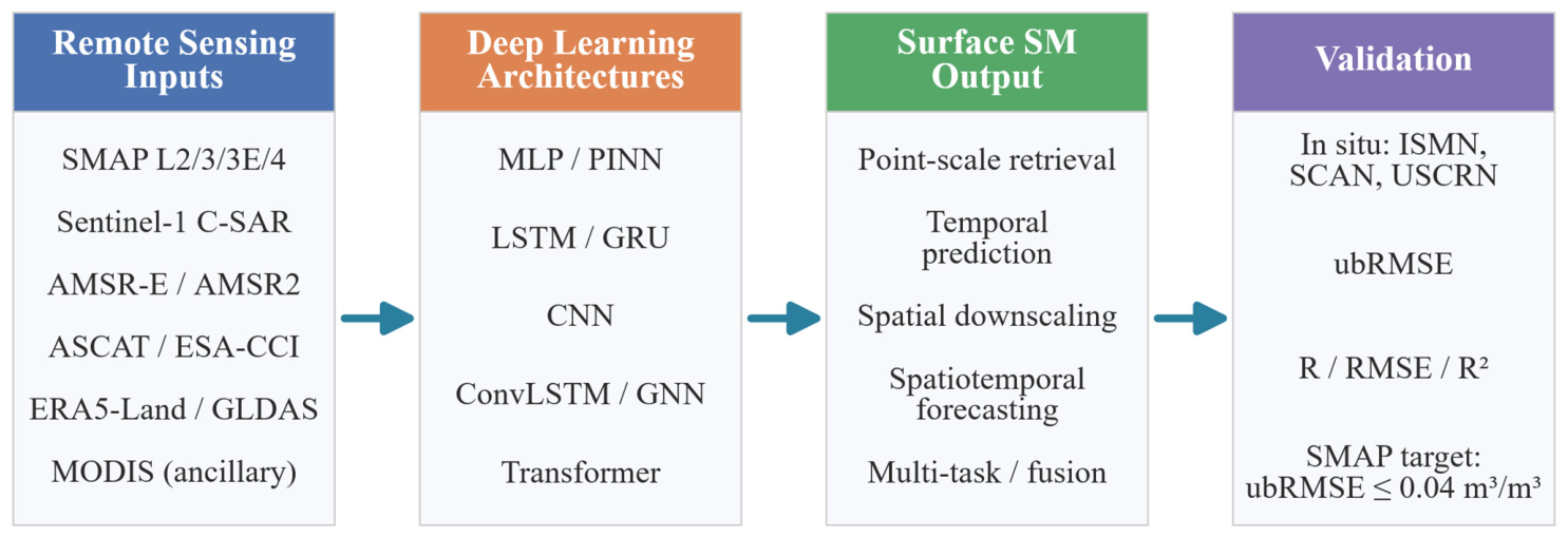Figure 1 illustrates this integrated research workflow, from multi-sensor satellite inputs through each architecture family to validated surface SM outputs.

3. Deep Learning Applications to Soil Moisture Remote Sensing

This section surveys how each deep learning family has been applied to remote sensing-based SM monitoring and prediction. Studies are grouped by dominant architecture: MLP and physics-informed neural networks (Section 3.1), LSTM- and GRU-based temporal models (Section 3.2), CNN-based SMAP downscaling (Section 3.3), spatiotemporal ConvLSTM and graph neural networks (Section 3.4), and Transformer-based multi-source fusion (Section 3.5). All reviewed studies adopt volumetric water content as the target variable and use ubRMSE, RMSE, R, or R² as primary metrics (Table 1). 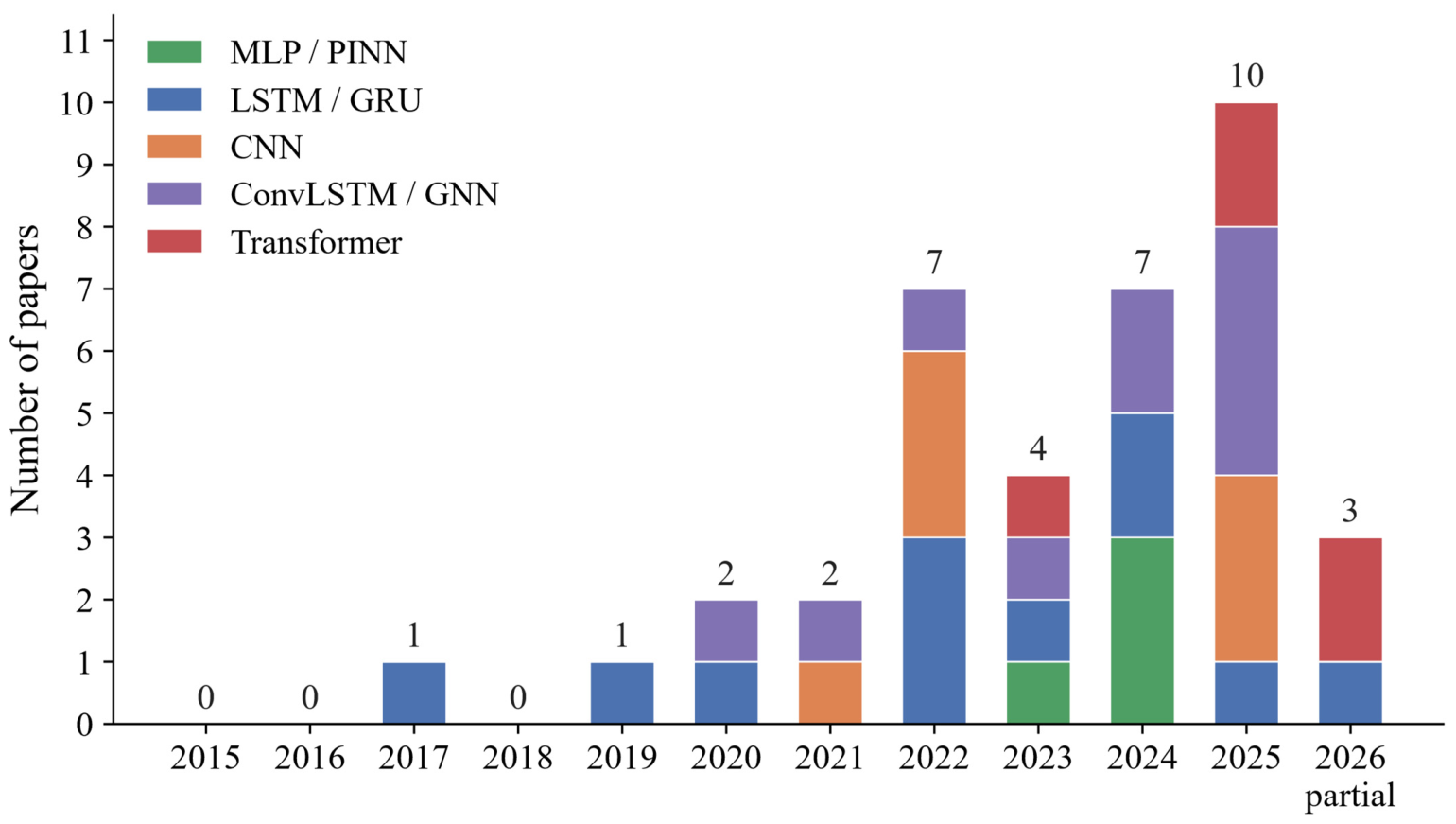Figure 2 summarizes the annual distribution of these studies across architecture families. It includes the single eligible 2017 study [5], indicates that no eligible core studies were identified for 2015–2016 or 2018, and marks 2026 as partial.

3.1. MLP and PINN for Surface Soil Moisture Retrieval

Among MLP-family architectures for surface soil moisture retrieval, this section surveys four studies spanning a spectrum from purely data-driven to physics-constrained approaches. Arab et al. [28] and Singh and Gaurav [29] demonstrate that shallow ANNs can achieve competitive accuracy over agricultural and alluvial landscapes using multi-source satellite inputs. Building on this data-driven foundation, Singh and Gaurav [30] incorporate SAR backscattering physics into the training objective of a feedforward network, while Li et al. [31] embed the water cloud model as a differentiable physical skeleton, enabling end-to-end physics-guided retrieval.

Singh and Gaurav [29] trained a fully connected ANN on nine satellite-derived features (dual-polarized Sentinel-1 SAR backscatter, Sentinel-2 red and near-infrared reflectance, and SRTM-derived elevation, slope, and fusion indices) to estimate surface SM across the 10,351 km² Kosi Fan alluvial system in northern Bihar, India. Validated against 224 TDR field measurements across two campaigns (December 2019 and March 2022), the model achieved R = 0.80 and RMSE = 0.040  ${\mathrm{m}}^3\hspace{0.17em}{\mathrm{m}}^{-3}$, outperforming all ten benchmark algorithms, including generalized regression neural networks, Gaussian process regression, random forests, support vector regression, and automated machine learning, with results stable across 30 independent data partitions. Feature importance analysis identified dual-polarization SAR backscatter and near-infrared reflectance as the dominant predictors; topographic slope contributed as an indirect moisture redistributor. The reported RMSE indicates competitive total-error performance, but because bias and ubRMSE were not reported separately, the result cannot be directly evaluated against the SMAP mission accuracy target.

Arab et al. [28] addressed the loss of high-resolution surface SM retrieval capability following the SMAP radar failure by integrating Sentinel-1A C-band SAR with the SMAP L-band radiometer. The coarse-resolution (9 km) SMAP Level-3 brightness-temperature data were first downscaled to 1 km using a Smoothing Filter-based Intensity Modulation (SFIM) algorithm that modulates SMAP brightness temperature by the ratio of the original and low-pass-filtered SAR backscatter coefficients. A multilayer perceptron (MLP) trained with the Levenberg–Marquardt algorithm then exploited the synergy between downscaled SMAP brightness temperatures, Sentinel-1A VH and VV backscatter, VIIRS land surface temperature, and the NDVI to retrieve surface SM at a 1 km resolution over agricultural fields in the Mississippi Delta during the 2016 growing season. Among the sensor combinations tested, VH-polarized Sentinel-1A provided the strongest complementary signal to the SMAP radiometer (R = 0.81), demonstrating that a passive-active multi-sensor MLP fusion strategy can partially restore the spatial resolution originally envisioned for the SMAP mission.

Singh and Gaurav [30] introduced PIML-SM, a physics-informed machine learning framework that incorporates SAR backscattering physics directly into the training objective of a shallow feedforward neural network. The architecture is a compact 9:3:1 feedforward neural network (nine satellite-derived inputs from Sentinel-1/2 and SRTM DEM, one hidden layer of three neurons, and one SM output). A physics term was added to the standard data-fitting loss by requiring the theoretically computed VV backscatter coefficient from the improved integral equation model (I²EM) to match the satellite-observed VV, simultaneously constraining predictions to remain physically consistent with surface roughness and soil dielectric properties. Parameters were optimized using particle swarm optimization (PSO). Trained on only 78 in situ measurements on the Kosi Fan—65% fewer than the data-driven ANN baseline [29]—PIML-SM achieved R = 0.94 and RMSE = 0.019  ${\mathrm{m}}^3\hspace{0.17em}{\mathrm{m}}^{-3}$, a 50% reduction in prediction error relative to the black-box ANN, while maintaining generalizability across contrasting climatic conditions (Bhopal, semi-arid: R = 0.97, RMSE = 0.010  ${\mathrm{m}}^3\hspace{0.17em}{\mathrm{m}}^{-3}$).

Li et al. [31] constructed a differentiable model (DM) for 10 m resolution surface SM retrieval by embedding the water cloud model (WCM) as a differentiable physical skeleton within PyTorch (https://pytorch.org). Two neural subnetworks parameterize the WCM: a fully connected network estimates static vegetation and soil parameters, while an LSTM estimates dynamic vegetation state variables; the analytically intractable bare-soil scattering component is replaced by a third fully connected network. The complete system is trained end-to-end via gradient descent without requiring separate supervised labels for intermediate outputs. Evaluated across four climatically diverse study areas—the Luan River Basin, Shandian River Basin, Maqu (Tibetan Plateau), and Lake Tahoe—the DM achieved a site-based R of 0.747–0.853 and an ubRMSE of 0.04539–0.05455  ${\mathrm{m}}^3\hspace{0.17em}{\mathrm{m}}^{-3}$, broadly comparable to random forest. In a stricter spatial extrapolation test using quadrats entirely withheld from training, DM outperformed all purely data-driven baselines with a median R = 0.786 and an ubRMSE = 0.05523 ${\mathrm{m}}^3\hspace{0.17em}{\mathrm{m}}^{-3}$, confirming that physical embedding substantially improves generalization in unseen environments.

3.2. LSTM- and GRU-Based Temporal Soil Moisture Prediction

The gated memory architecture of LSTM is particularly well suited to SM time-series prediction: its cell states encode the multi-day hydrological memory of surface SM, capturing how precipitation impulses attenuate over timescales from hours to weeks. This section traces the development of LSTM- and GRU-based SM applications from their inception as SMAP gap-filling tools, through multiscale satellite–in situ fusion frameworks, to recent extensions addressing physics-guided loss design, hybrid physics-DL integration, training data imbalance, and interpretable transfer learning across climatic regimes.

3.2.1. Pioneer LSTM Applications for SMAP Temporal Extension

Fang et al. [5] first applied LSTM to continental-scale SMAP SM temporal gap-filling, training the network to predict the SMAP Level-3 passive surface SM product across CONUS using atmospheric forcing (NLDAS-2), static physiographic attributes, and Noah land surface model (LSM)-simulated moisture as inputs. The model achieved an RMSE < 0.035  ${\mathrm{m}}^3\hspace{0.17em}{\mathrm{m}}^{-3}$ and an R > 0.87 for more than 75% of the CONUS pixels, including the forested southeastern United States. Generalization was held across both temporal and regional holdout experiments spanning hydrologically distinct HUC-2 basins. A single weight set trained over one year generalized accurately to subsequent years.

Subsequently, Fang et al. [32] investigated whether LSTM-prolonged SMAP data provides added value beyond LSM simulations. To measure the value of independent remote-sensing information, they excluded Noah-simulated variables from the LSTM inputs. Although LSTM’s performance ceiling was constrained by SMAP’s shallow sensing depth, a simple ensemble average of LSTM and Noah outputs (denoted as “Comb”) frequently outperformed Noah alone, with the advantage more pronounced at sparsely instrumented sites. The LSTM successfully reproduced long-term interannual surface SM trends from SMAP observations across multi-year projection windows with negligible performance degradation, establishing temporal hindcasting as a core capability of recurrent SM architectures.

Fang and Shen [33] addressed the near-real-time operational constraint of producing SM nowcasts despite SMAP’s approximately 67% data missing rate by augmenting the standard LSTM with an adaptive data integration (DI) kernel. This DI kernel injects the most recently available SMAP observation as an additional input through a closed-loop procedure: when no observation is available, the network’s own previous prediction serves as the default data-injection term, enabling continuous gap-bridging without offline interpolation that would leak future information. Evaluated over CONUS, DI-LSTM outperformed prior near-real-time methods reported in the literature, with its comparative advantage becoming more pronounced at longer forecast latencies. The DI procedure also removed autocorrelated forcing errors, preventing them from accumulating or persisting due to unrepresented physical processes such as irrigation, floodplain inundation, and lake dynamics. This adaptive framework, insensitive to irregular observational schedules, established an automated template for sequential deep learning in near-real-time satellite SM forecasting.

3.2.2. Multiscale and Multi-Source LSTM for Large-Scale SM Mapping

Liu et al. [34] proposed a multiscale LSTM framework to reconcile SMAP’s coarse 36 km footprint with 9 km in situ station networks. Sixteen fine-resolution (9 km) LSTM models operate in parallel within each 36 km SMAP grid cell, sharing a uniform set of weights while receiving location-specific NLDAS-2 meteorological forcing and terrain attributes. The loss function jointly penalizes discrepancies between aggregated fine-scale predictions and SMAP L3 retrievals, and between individual fine-scale predictions and ground observations (from USCRN, SCAN, and CVS). The resulting daily 9 km CONUS product achieved a median RMSE = 0.034  ${\mathrm{m}}^3\hspace{0.17em}{\mathrm{m}}^{-3}$ and R = 0.901 against USCRN, outperforming standalone SMAP products, single-scale DL models, and land surface models.

Utilizing globally distributed stations, Celik et al. [35] trained a two-hidden-layer LSTM framework tailored for field-scale SM prediction. The model ingested a multi-source dataset comprising Sentinel-1 backscatter (VV, VH, VH/VV), SMAP surface and subsurface SM, climate variables, soil texture fractions, and four topographic attributes, validated against active ISMN stations after 2017. On the daily test set, the model achieved RMSE = 0.046  ${\mathrm{m}}^3\hspace{0.17em}{\mathrm{m}}^{-3}$, ubRMSE = 0.045  ${\mathrm{m}}^3\hspace{0.17em}{\mathrm{m}}^{-3}$, and R² = 0.87. Performance was optimal under arid (Bw) climate conditions but deteriorated under high vegetation cover (high NDVI) due to biomass-induced signal scattering.

O et al. [36] developed a high-resolution European daily SM dataset (SoMo.ml-EU, 2003–2020) using an LSTM-based framework, producing a 0.1° daily product across three vertical layers. The higher-resolution product agreed more closely with independent in situ measurements than its 0.25° predecessor. The improvement is particularly pronounced in capturing SM variability, including drought conditions. Jointly processing in situ observations with high-resolution meteorological forcings allows the model to better mirror the fine-scale spatial footprint of field data and resolve sub-grid hydroclimatic variations.

3.2.3. Physically Guided, Hybrid, and Transfer Learning Extensions

Geng et al. [37] addressed the absence of physical priors in data-driven SM modeling by introducing two physically guided loss functions into the standard LSTM training objective. PHY-LSTM encodes a penalty term enforcing the monotonic relationship between the surface water balance budget (inflow minus outflow) and shallow SM; PHYS-LSTM extends this constraint to deep soil water. Both architectures were trained on the global ERA5-Land dataset for next-day surface SM forecasting without changing the underlying recurrent network structure. Compared to the conventional data-driven LSTM, both models achieved substantial and closely comparable performance gains. PHYS-LSTM improved over the standard LSTM by KGE +13.6%, R² +20.7%, and RMSE −8.2%, confirming that embedding soft physical constraints as regularized loss terms enhances both predictive accuracy and geographical generalization across diverse global climate conditions.

Li et al. [38] developed a hybrid prognostic framework for 1–16-day SM forecasting over China by adaptively integrating outputs from the physics-based Global Forecasting System (GFS/Noah LSM) into a ConvLSTM encoder–decoder model. An attention block computed channel-wise weights from the GFS forecast tensors at each prediction time step, routing selectively weighted physical priors into the recurrent decoder to reduce spatial and temporal systematic errors. To improve generalization, the authors built an ensemble scheme combining the average, condition, and attention-based hybrid variants. Trained on SMAP L4 daily estimates (9 km resolution) with embedded GEOS climate forcings, the ensemble model broke the default training data ceiling, outperforming the pure DL baseline across more than 79.5% of in situ verification stations for 16-day long-term forecasts. The attention variant also showed higher predictability during extreme drought events, exploiting the physics-based background to capture slowly evolving SM deficits that purely data-driven networks typically underweight.

Li et al. [39] identified a structural training problem in global LSTM-based SM prediction: the distribution of SM values is highly imbalanced, making moderate moisture states orders of magnitude more common than extreme dry or wet conditions and causing standard training to be poorly calibrated at the climatological tails. The authors corrected this imbalance with a Sampling-Weighted Sensitive Learning Strategy, using Gaussian kernel density estimation to quantify the global SM distribution and up-weighting rare extreme samples during back-propagation. Applied to LSTM, BiLSTM, and GRU architectures trained on ERA5-Land, the strategy improved BiLSTM performance by ubRMSE −7.38%, Bias −11.64%, and KGE +2.73%, with KGE gains exceeding 20% in North Africa and West Asia, where extreme moisture anomalies dominate hydrological variability.

Ye et al. [40] examined how pre-trained Bi-LSTM knowledge transfers across contrasting hydrological regimes for subsurface SM prediction (7–28 cm depth), training on the semi-arid Yellow River Basin (YRB) and transferring to Jianpinggou (JPG), a humid headwater catchment in southwestern China with limited in situ data. The transferred model outperformed a model trained exclusively on local JPG data and improved further after lightweight fine-tuning with a small in situ set. SHapley Additive exPlanations (SHAP) analysis revealed a mechanistic regime shift: evapotranspiration dominated subsurface SM prediction in the dry YRB, whereas soil matrix flux signals (surface SM and precipitation lags) dominated in the humid JPG. The contrast suggests that fine-tuning adapts the learned feature-relevance hierarchy to the target regime rather than merely recalibrating numerical outputs. Although the target depth extends below the surface layer, this study is included for its demonstration of explainable BiLSTM transfer learning methodology, which is directly applicable to surface SM estimation under data-sparse conditions.

Nijaguna et al. [41] targeted SM retrieval in vegetated areas by coupling an improved physics-based water cloud model (WCM) with a hybrid architecture consisting of a Bidirectional GRU (Bi-GRU) and a Deep Maxout Network (DMN). Four distinct vegetation indices (NDVI, GLAI, GNDVI, and WDRVI) derived from satellite data were utilized to parameterize the WCM vegetation impact rectification scheme. Both the extracted vegetation features and the vegetation-corrected radar backscatter coefficients were fed in parallel into the Bi-GRU and DMN streams, with their respective outputs combined via an enhanced score-level fusion mechanism. This integrated framework reduced retrieval errors relative to conventional methods and traditional WCM variants, with the largest gains in densely vegetated pixels where canopy scattering most severely contaminates the SAR signal.

Yu et al. [42] integrated physical WCM constraints into an LSTM model for field-scale SM retrieval from Sentinel-1 SAR in the Yanco agricultural region of southeastern Australia. WCM-decomposed soil backscatter coefficients, derived by separating the Sentinel-1 signal into vegetation and soil contributions using NDVI-derived vegetation water content, were fed into an LSTM alongside Landsat surface characteristics; a dual-component loss function combined a WCM-based semi-physical term with the standard data-fitting MSE. Four-fold spatial cross-validation against OzNet in situ measurements showed that the WCM-guided LSTM achieved an RMSE of 0.06–0.08 ${\mathrm{m}}^3\hspace{0.17em}{\mathrm{m}}^{-3}$ and an R of 0.40–0.64, improving on standalone WCM (RMSE 0.08–0.10 ${\mathrm{m}}^3\hspace{0.17em}{\mathrm{m}}^{-3}$, R 0.26–0.34) and reducing retrieval uncertainty by 0.02. As a preliminary six-page IGARSS 2025 conference study, the approach warrants further validation at broader scales and across diverse agricultural landscapes before operational deployment.

Across these studies, LSTM- and GRU-based approaches demonstrate a clear capability progression: from SMAP temporal gap-filling and nowcasting at the CONUS scale [5,32,33], through multiscale satellite–in situ fusion at 9 km resolution [34] and multi-source field-scale mapping [35,36], to physics-embedded loss functions [37], hybrid physics-DL integration for extended forecast horizons [38], sampling-weighted training to improve predictions at moisture extremes [39], interpretable cross-regime transfer learning [40], vegetation-corrected radar retrieval [41], and WCM-guided LSTM for field-scale SAR SM retrieval [42]. Recurrent architectures provide strong total-error references under favorable multiscale constraints [34] (RMSE = 0.034  ${\mathrm{m}}^3\hspace{0.17em}{\mathrm{m}}^{-3}$) while remaining separate from the SMAP ubRMSE mission benchmark unless ubRMSE is explicitly reported. These models also consistently outperform non-temporal feedforward models at extended prediction horizons. These spatial resolution constraints motivate the CNN-based downscaling strategies in Section 3.3.

3.3. CNN-Based SMAP Spatial Downscaling

The coarse spatial resolution of SMAP Level-3 products (36 km) limits their utility for sub-field and watershed-scale applications, motivating CNN-based downscaling research that uses high-resolution auxiliary observations (land surface temperature, surface reflectance, topography, and soil texture) to disaggregate passive microwave SM to 1–3 km daily products. This section reviews the progression from foundational pixel-neighborhood CNN approaches through multi-source deep neural network (DNN) fusion and physically informed DenseNet architectures, tracing how each generation addresses scale mismatch, interpretability, and accuracy degradation that constrain purely statistical downscaling.

3.3.1. Convolutional and Wide-Deep Architectures for SMAP Downscaling

Xu et al. [43] proposed a map-to-pixel CNN downscaling framework for SMAP, replacing the conventional pixel-to-pixel strategy with spatially aware convolutions that exploit information from adjacent pixels. The model accepted stacked MODIS surface reflectance (seven bands, MOD09GA at 500 m) and land surface temperature (MOD11A1 at 1 km) as inputs, incorporated a dedicated weight layer for input channels to mitigate padding errors, and predicted residual SM to ensure spatial consistency. Applied to a regional subset of the South-Central United States containing 109 Oklahoma Mesonet stations as ground truth for 2018, the optimal network version (CNN_N) generated 3 km and 1 km downscaled products from the 9 km SMAP L3_SM_P_E Enhanced product. The 3 km product achieved a mean RMSE = 8.34% and an ubRMSE = 4.97%, tightly matching the accuracy of the original 9 km product (RMSE = 8.35%, ubRMSE = 4.95%), whereas the accuracy at 1 km degraded markedly (RMSE = 8.40%, ubRMSE = 5.18%), establishing 3 km as the effective resolution ceiling for this input feature set. Pixel-neighborhood convolution added significant value over single-pixel regression, but the available auxiliary features were insufficient to sustain high accuracy beyond the 3 km threshold.

Xu et al. [44] extended satellite spatial downscaling to the 36 km → 1 km scale by adopting a Wide-and-Deep Learning (WDL) architecture over the Continental United States (CONUS) for the April-to-November unfrozen season. To balance memorization and generalization, the deep component captures complex, non-linear feature interactions from 14 high-dimensional environmental covariates via successive hidden dense layers. Meanwhile, the wide linear component places explicit training emphasis on the three most highly correlated driving factors (Soil pH, TBv, and TVMDI) by assigning them higher regional weights. The unified architecture is trained directly against the coarse-resolution 36 km SMAP L3_SM_P product. When cross-validated against independent in situ ground truth from 211 ISMN stations, the downscaled 1 km composite map achieved an average ubRMSE of 0.041 ${\mathrm{m}}^3\hspace{0.17em}{\mathrm{m}}^{-3}$. This reported ubRMSE is close to the SMAP mission accuracy target (~0.04 ${\mathrm{m}}^3\hspace{0.17em}{\mathrm{m}}^{-3}$) while preserving the spatial macro-trends of the original passive microwave asset.

3.3.2. Deep Belief Networks and Architecture Comparison for Complex Terrain

Zhao et al. [45] benchmarked three DL configurations (Deep Belief Network, neighborhood-constrained DBN, and ResNet) against two conventional methods (BPNN and Random Forest) for 36 km → 1 km SMAP downscaling on the Tibetan Plateau, a region of intense elevation gradients, frozen soil, and sparse in situ networks. ResNet achieved the highest stability across validation networks, while all DL methods produced more spatially coherent patterns and finer texture detail than BPNN and RF, particularly in high-uncertainty areas associated with elevation-driven SM gradients. The neighborhood-constrained DBN, which incorporates spatial adjacency information into the DBN feature extraction, improved over the standard DBN in rugged sub-regions, indicating that receptive-field size is a critical design parameter in mountainous terrain where SM heterogeneity is strongest.

Dastbala et al. [46] applied a Deep Belief Network (DBN) for 36 km → 3 km spatial downscaling of SMAP soil moisture over the western United States. The model utilized resampled auxiliary factors, including SMAP brightness temperatures (TBh and TBv), MODIS LST, NDVI, albedo, CHIRPS precipitation, and GTOPO30 DEM, as soil moisture proxies. During the testing phase, the DBN achieved the best performance (R = 0.96), outperforming random forest (R = 0.93), ANN (R = 0.82), and linear regression (R = 0.65). Permutation Feature Importance (PFI) identified TBv as the most critical predictor, whereas the NDVI exhibited the lowest significance, potentially due to scaling-induced non-linear errors or topographic-ecological trade-offs in complex networks. Ablation analysis confirmed that sequentially removing the five least significant proxies optimizes the balance between accuracy and model simplicity. Finally, land-cover-stratified evaluation against SNOTEL in situ measurements revealed marked performance variations, with grasslands showing the highest correlation (R = 0.75) and tree cover the lowest (R = 0.30), reinforcing the necessity of stratified validation for downscaled remote sensing products.

3.3.3. Multi-Source DNN Fusion and Physics-Guided DL for High-Fidelity SM Products

Gao et al. [47] addressed the underperformance of SMAP L-band retrievals over densely vegetated land covers (vegetation water content exceeding 5 kg m⁻²) by training a DNN to integrate the complementary strengths of three SMAP L3 SM products (SCA-V, SCA-H, and DCA) and ERA5 reanalysis. Satellite SM provides lower absolute bias than reanalysis but insufficient temporal co-variability with in situ measurements, particularly over non-cropland, whereas ERA5 offers better temporal variability but spatially varying systematic errors. ERA5 SM, alongside SMAP products, was used to construct a bias-adjusted target benchmark stratified by land cover rather than acting as a direct network input. Supplied with 10 physical predictors, including SMAP polarized brightness temperatures, effective soil temperature, vegetation scattering albedo, surface roughness, soil attributes, and vegetation optical depth (VOD) climatology, the DNN was trained on 2015–2017 data. When evaluated on a four-year independent testing period (2017–2021) against global ISMN stations, the framework achieved a cross-validation RMSE = 0.036  ${\mathrm{m}}^3\hspace{0.17em}{\mathrm{m}}^{-3}$, outperforming individual SMAP algorithms and ERA5 across most land cover and climate strata.

Coupling DenseNet with thermal inertia (TI) theory, Xu et al. [48] improved interpretability in a Wide-and-Deep downscaling framework. Thermal inertia (TI) quantifies a soil’s resistance to diurnal temperature change; wet soils exhibit larger TI and smaller diurnal land surface temperature differences (ΔT), providing a physically grounded indirect proxy for SM. Daily gap-free LST and its derived ΔT were reconstructed using a CFSv2-SG approach that fills MODIS cloud gaps via CFSv2 model temperatures followed by Savitzky–Golay smoothing. In the joint network, ΔT acts as a physically explicit input for a wide linear regression to constrain the outputs, while also feeding into the Deep DenseNet branch alongside SMAP brightness temperatures, MODIS EVI, topography, and soil attributes. Categorical attributes (land cover and climate type) were processed via one-hot encoding. While the model was trained on 36 km EASE-grid data from 2015 to 2018, it was independently validated against 264 point-scale ISMN stations for the April–November 2015 season. The downscaled 1 km daily SM achieved a mean ubRMSE of 0.048 ${\mathrm{m}}^3\hspace{0.17em}{\mathrm{m}}^{-3}$, enabling non-linear feature reuse while maintaining physical accountability.

Sub-pixel SM heterogeneity was the target of Moosavi et al. [49], who partitioned the study region into homogeneous clusters and trained separate deep learning models within each through the Cluster-Based Local Modeling (CBLM) framework. Applied over the Maragheh Basin in Iran using Sentinel-2 imagery, in situ TDR measurements, and topographic environmental ancillary data, the CBLM approach outperformed global modeling baselines. A hybrid CNN-LSTM trained within this cluster-local scheme achieved the highest estimation accuracy (R² = 0.98). The cluster-local structure captures localized SM dynamics that global networks average out; using separate models for distinct soil and environmental units further improves physical consistency and interpretability.

CNN-based downscaling has advanced SMAP SM from the 36 km mission grid to 1 km daily fields, but reported accuracy must be interpreted by metric type. Xu et al. [44] reported an ubRMSE = 0.041  ${\mathrm{m}}^3\hspace{0.17em}{\mathrm{m}}^{-3}$, close to the SMAP ubRMSE target, whereas Gao et al. [47] reported an RMSE = 0.036  ${\mathrm{m}}^3\hspace{0.17em}{\mathrm{m}}^{-3}$ as a total-error metric. Key architectural choices determine where accuracy limits fall. Pixel-neighborhood convolution sets the recoverable spatial ceiling at approximately 3 km, given standard MODIS auxiliary inputs [43]; Wide-Deep joint training handles mixed memorization and generalization across diverse CONUS conditions [44]; ResNet provides the most stable 1 km products on complex terrain [45]; DBN, with physical brightness-temperature inputs, reveals high sensitivity to land cover stratification [46]; multi-source DNN fusion reduces systematic vegetation-cover bias over multiple unseen test years [47]; and TI-guided DenseNet offers the clearest physical interpretability while maintaining competitive accuracy [48]. Hybrid CNN-LSTM architectures trained under cluster-local schemes also capture watershed-scale heterogeneity more accurately [49]. Persistent limitations include near-universal accuracy degradation at the 1 km scale without additional sub-pixel physical constraints, seasonal data gaps during frozen periods, and restricted geographical transferability for globally uniform models, all of which motivate the spatiotemporal and graph-based architectures reviewed in Section 3.4.

3.4. Spatiotemporal Deep Learning: ConvLSTM and Graph Neural Networks

ConvLSTM substitutes spatial convolutions for the fully connected operations in standard LSTM gates, so each recurrent step processes a location in the context of its spatial neighborhood. This makes the architecture well suited to gridded SM fields, where moisture patterns evolve with some spatial coherence across time steps. GNNs take a different approach: rather than operating on a regular grid, a GNN defines connectivity through an explicit adjacency matrix, routing information between any pair of stations regardless of their distance in grid space. Section 3.4 reviews ConvLSTM applications to SM prediction and gap-filling, physics-prior and data integration extensions, and GNN architectures for sensor-network SM estimation.

3.4.1. ConvLSTM for Spatiotemporal SM Prediction and Gap-Filling

ElSaadani et al. [50] first applied ConvLSTM to hourly SM predictions and temporal gap-filling in south Louisiana, a flood-prone region where rapid SM dynamics are safety-critical. Using the National Water Model Noah-MP LSM outputs as the reference target, the models utilized static land cover data, radar rainfall, and up to five dynamic hydrometeorological predictors (longwave/shortwave radiation fluxes, moisture availability, storm surface runoff, and baseflow runoff). ConvLSTM outperformed the standalone CNN baseline; incorporating temporal memory improved hydrologic predictions beyond what the spatial-only CNN achieved. Sensitivity experiments revealed that a shorter antecedent sequence (3 h) in an exclusive setup yielded the best performance, achieving a mean areal correlation coefficient of 0.9 and a mean areal RMSE of 2.5%. The approach also generated continuous hourly predictions between the 3-hourly reference observations, filling temporal gaps in satellite coverage.

Foley et al. [51] proposed the SMArtCast pipeline, combining a sequence-to-sequence LSTM encoder–decoder framework with standard Gaussian kriging interpolation to predict spatially dense SM maps at multiple depths up to 14 days into the future. A separate seq2seq LSTM encoder–decoder forecasts future pixel-wise NDVI and NDWI imagery from five historical satellite acquisitions, with temporal encoding (days to target date) handling the irregular revisit cycles of satellite observations. Independently, a separate LSTM model ingested dynamic meteorological variables and salinity data to predict future daily SM values at sparse in situ sensor locations across 10–120 cm depths, achieving a 14-day testing RMSE range of 0.4–2.4% (mean 1.23%) against a baseline soil moisture variability of 15–60%. These future point predictions and distance-based vectors were then mapped across the predicted satellite imagery background using Gaussian kriging, yielding high interpolation scores of 0.82–0.97 across all depths. While this framework successfully fills temporal gaps in remote sensing and extends projections into future weeks, its operational implementation relies on traditional spatial interpolation algorithms rather than an end-to-end spatiotemporal deep learning model.

Zhu et al. [52] benchmarked four spatiotemporal architectures for SM prediction on the North China Plain, China’s most agriculturally productive region, training and evaluating ConvLSTM, Memory in Memory (MIM), PredRNN, and CubicRNN on ERA5 reanalysis and CN05.1 meteorological data. ConvLSTM achieved the lowest prediction errors on both single-time-step and multi-step spatiotemporal metrics. However, all four architectures showed markedly increased errors when SM values exceeded the 75% percentile interval. This elevated error reflects a shared difficulty in predicting extreme wet events, consistent with the training data imbalance problem documented for LSTM-based methods (Section 3.2).

For a safety-critical downstream application, Hosseinizadeh et al. [53] generated high-resolution spatiotemporal SM maps for Prince George’s County, Maryland, to improve infiltration modeling for landslide risk assessment. Self-calibrated Sentinel-1 change-detection products served as training labels, providing dense, high-resolution SM labels without relying on sparse in situ measurements. The ConvLSTM integrated static spatial features (elevation, slope, and soil type) with multi-temporal meteorological inputs (precipitation, temperature, humidity, wind speed, and evapotranspiration) and temporal vegetation coverage to capture both topographically mediated redistribution infiltration and storm-event dynamics. Validated against Sentinel-1-derived SM, the model achieved R² = 0.72 and R = 0.85, which are sufficient for slope stability assessments but at a spatial resolution unavailable from passive microwave missions.

3.4.2. Spatiotemporal DL with Data Integration and Physical Priors

Zhang et al. [54] advanced real-time SM forecasting by incorporating a ConvGRU backbone into a data integration framework, developing the DI_ConvGRU model to supplant point-to-point temporal models like DI_LSTM. This architecture captures both the spatial distribution of SM across the target domain and its temporal persistence via gated recurrence. Formulated over China (18–54° N, 73–135° E), the model utilizes 1-day lagged SMAP L3 SM, 1-day lagged ERA5-L and meteorological forcing, and static physiographic attributes as predictors to forecast future SM. To address prevalent satellite data gaps, the DI scheme recursively substitutes missing lagged observations with the model’s prior predictions during training. DI_ConvGRU achieved an ubRMSE of 0.022 ${\mathrm{m}}^3\hspace{0.17em}{\mathrm{m}}^{-3}$ on the test set, outperforming interp_ConvGRU and DI_LSTM across 74.88% and 68.99% of the study region, respectively. The performance advantage over both interpolation-based ConvGRU and DI-LSTM demonstrates the contribution of spatial convolution to the data integration framework.

Sivaprasad et al. [55] produced a seamless continental-scale AMSR-E/2 surface soil moisture time series spanning 2003–2023 over Europe using a hybrid ConvLSTM2D-Conv2D model and transfer learning. The framework was first trained to predict AMSR-2 SM by utilizing ASCAT SM alongside land mask and cyclical day-of-the-year encodings as input features, deliberately excluding meteorological variables like precipitation to maintain independence for subsequent land surface model assimilation. Transfer learning then adapted this pre-trained model to gap-fill the older AMSR-E data, establishing a consistent sensor-bridging target. Validated against 137 ISMN stations across Europe, the enhanced product demonstrated a 26% improvement in correlation with in situ measurements compared with the original products, providing a gap-free, reanalysis-ready dataset.

3.4.3. Graph Neural Networks for SM Spatial Prediction

Pan et al. [56] addressed the limitations of ConvLSTM in capturing heterogeneous dependencies from spatially remote locations by proposing GCCL, a deep learning model that integrates a Graph Convolutional LSTM (GConvLSTM) and a convolutional LSTM (ConvLSTM) branch through a layered memory-flow architecture. Instead of a simple parallel structure, GConvLSTM passes its hidden states vertically to ConvLSTM, while ConvLSTM feeds its temporal information back to guide GConvLSTM. GConvLSTM constructs a connectivity matrix based on Pearson correlation coefficients to identify the top seven nodes with the highest temporal correlation, routing long-range spatial information through a normalized k-hop graph convolution. In parallel, the ConvLSTM branch captures localized spatiotemporal patterns. Trained on historical 3-day sequences of SMAP L4 SM (9 km, daily) and five selected ERA5-Land predictors retained after multi-collinearity screening, GCCL achieved a Lead-1 Day RMSE of 0.018 ${\mathrm{m}}^3\hspace{0.17em}{\mathrm{m}}^{-3}$. It outperformed the standalone ConvLSTM in 98% of the region, achieving a 14.3% RMSE reduction.

Wang et al. [57] proposed a spatiotemporal graph convolutional network, designated as SMF4WSN, for SM forecasting within the SMN-SDR, a wireless sensor network comprising 34 stations and covering approximately 10,000 km² in the ShanDian River basin. Although the raw telemetry was sampled at 10–15 min intervals, the data were temporally aggregated and resampled to a 4 h resolution for model input, capturing SM at a 3 cm depth, as well as soil temperature and precipitation. The SMF4WSN architecture uses graph convolutions to encode spatial topology and gated convolutional neural networks to capture temporal dynamics. Compared to two baseline models (LSTM and random forest), SMF4WSN improved prediction accuracy by 49.53%, 34.86%, and 29.73% at the 12-step (48 h), 36-step (144 h), and 48-step (192 h) forecast horizons, respectively, with an overall correlation coefficient of 0.94. The performance advantage holds as the forecast horizon extends, indicating that graph-encoded spatial context reduces long-term error accumulation.

Vyas and Bandyopadhyay [58] formulated SM prediction as a semi-supervised learning problem on dynamic graphs, proposing DGLR, a dynamic GNN framework that jointly learns graph structures and SM values in an end-to-end fashion. Recognizing that geographic proximity does not guarantee SM co-variability due to abrupt soil-type or landscape transitions, DGLR optimizes a reconstructed adjacency matrix driven by node embedding similarities rather than relying purely on static spatial heuristics. Spatial and temporal dependencies are captured through stacked self-attention GNN and GRU layers, utilizing separate GRU parameters per location to preserve highly localized temporal trends. This semi-supervised framework uses data from both monitored and unmonitored locations via message passing. Evaluated on datasets integrating remote sensing (MODIS NDVI, Sentinel-1 SAR) and IBM weather data, DGLR achieved state-of-the-art forecasting performance over conventional ML baselines, offering an effective approach for precision agriculture.

ConvLSTM and GNN architectures extend SM prediction capabilities in complementary directions. ConvLSTM directly encodes the spatiotemporal co-evolution of gridded SM fields, enabling high-frequency temporal gap-filling [50] and gap-free multi-sensor time-series production via transfer learning [55]. GNNs explicitly represent inter-node dependencies through adjacency matrices, recovering the long-range spatial correlations missed by local convolutions, with data-driven Pearson adjacency [56] and learnable dynamic topology [58] both outperforming purely local baselines. One low-ubRMSE example in this section is DI_ConvGRU [54] (ubRMSE = 0.022  ${\mathrm{m}}^3\hspace{0.17em}{\mathrm{m}}^{-3}$). Whether graph adjacency learned from correlation generalizes across climate regimes remains an open question; the computational cost of global-scale ConvLSTM motivates the Transformer-based approaches reviewed in Section 3.5.

3.5. Transformer, Attention-Based, and Multi-Source Fusion Architectures for SM Estimation

Transformer architectures are built on multi-head self-attention, which establishes direct connections between arbitrary positions in the input sequence, enabling simultaneous modeling of long-range inter-variable correlations across irregular temporal sampling and multiscale spatial structures. This section reviews SM estimation methods that employ Transformer self-attention [59,60], cross-attention multi-source fusion [61,62], and convolutional regression multi-source integration [63].

3.5.1. Transformer Networks for Global SM Simulation and SMAP Enhancement

Liu et al. [59] applied a Transformer-based SM Simulation Network (TSMSNet) to simulate future global surface SM (0–10 cm) from 2016 to 2099 under three CMIP6 Shared Socioeconomic Pathway (SSP) scenarios. To resolve the blurred variations inherent in traditional multi-model ensemble averages, TSMSNet was trained on 2015–2024 data using nine selected Earth System Models alongside their spatial error characteristics that were derived from extended triple collocation. The model learning target combined the strengths of the SMAP radiometer and ERA5-Land SM datasets. Validated against 670 global ISMN stations, TSMSNet achieved an ubRMSE of 0.045 ${\mathrm{m}}^3\hspace{0.17em}{\mathrm{m}}^{-3}$ and an R of 0.68, outperforming both its ConvLSTM counterpart (CSMSNet: R = 0.65, ubRMSE = 0.047  ${\mathrm{m}}^3\hspace{0.17em}{\mathrm{m}}^{-3}$) and simple ensemble means. The resulting projections revealed a consistent global drying trend across all SSPs, with habitable areas, croplands, and forests exhibiting the most severe moisture deficits, supporting century-scale agricultural drought assessment.

Liu et al. [60] developed SMSNet, a Transformer-based network that separates temporal and spatial self-attention into dedicated encoder modules, designed for both SMAP gap-filling at 9 km and spatial downscaling to 1 km. The dynamic feature extraction module processes 8 × 8-pixel spatiotemporal patch sequences (segmented into 4 × 4 patches and linearly embedded into a 256-dimensional space with spatiotemporal position encoding) across a five-day input window; a separate static feature encoder processes time-invariant attributes (DEM, soil properties, and land cover) through an independent Transformer, and the two representations are merged in a non-linear fusion module that outputs SM at the target resolution. Validated at SCAN and USCRN stations across CONUS (with LST filtering to exclude frozen conditions), SMSNet achieved RMSE = 0.086  ${\mathrm{m}}^3\hspace{0.17em}{\mathrm{m}}^{-3}$ and R = 0.639 on SCAN and RMSE = 0.097  ${\mathrm{m}}^3\hspace{0.17em}{\mathrm{m}}^{-3}$ and R = 0.665 on USCRN for the 9 km reconstruction product while exploiting scale consistency by directly applying the 9 km-trained model to 1 km inputs without additional fine-tuning. Because SMSNet reported the RMSE rather than ubRMSE, these errors are best interpreted as total-error reconstruction metrics rather than direct tests against the SMAP ubRMSE mission target. SMSNet’s primary contribution lies in its unified architecture for simultaneous SMAP gap-filling and spatial downscaling within a single Transformer framework, eliminating the need for scale-specific fine-tuning.

3.5.2. Cross-Attention and Multimodal Fusion for Multi-Source SM Reconstruction

Wang et al. [61] proposed a multi-source SM fusion framework combining a CNN-LSTM backbone with climate-zoning and auxiliary-guided cross-attention to reconstruct a continuous 72-year (1950–2021) daily SM dataset at 0.1° resolution over the Yellow River Basin. The study period was segmented into three chronological windows based on product availability (ERA5-L from 1950, ESA CCI from 1978, and SMAP from 2015) to maximize data utilization. Within this framework, a separate CNN first extracts hierarchical spatial features from individual soil moisture and auxiliary grids (precipitation, skin temperature, and elevation). A cross-attention module then dynamically reweights the SM product features by conditioning queries on the auxiliary environmental features to automatically capture the relative strengths of each source. These weighted features are concatenated with auxiliary features and fed into a bidirectional LSTM to model long-range temporal dependencies. Validated against 274 in situ stations across the basin (752,443 km²), the framework achieved an ubRMSE of 0.043 ${\mathrm{m}}^3\hspace{0.17em}{\mathrm{m}}^{-3}$, outperforming both the source products and the random-forest-based SMCI1.0 dataset (2000–2020).

Xu et al. [62] presented MMNet, a multimodal deep learning model that explicitly separates same-day snapshot observations from preceding 10-day environmental time series into two parallel encoding streams, addressing the limitation of methods that rely solely on instantaneous spectral snapshots. The snapshot encoder, a three-layer MLP, integrates coarse SMAP L4 surface SM with Landsat-8 indices (NDVI, EVI, NDWI, and LSWI), Sentinel-1 SAR metrics (CR, DPSVIm, Pol), and time-invariant soil and terrain properties to capture location-specific controls. A separate temporal encoder uses a Transformer to process a 10-day sequence of daily gridMet weather variables (including precipitation, radiation, humidity, and evapotranspiration) and MODIS LST, encoding the antecedent moisture state driven by weather history. A fusion layer combines both representations before a regression network outputs downscaled 100 m SM estimates. Three evaluation scenarios across SCAN and USCRN stations over CONUS showed that this snapshot–time-series integration was necessary for maintaining accuracy and generalizability in data-scarce regions, establishing MMNet as a generalizable framework for high-resolution agricultural and hydrological applications.

3.5.3. High-Resolution Global SM Retrieval via Multi-Source Deep Learning Fusion

Batchu et al. [63] developed a convolutional regression model that fuses inputs spanning three orders of spatial resolution (Sentinel-1 VV/VH SAR at 10 m, Sentinel-2 multispectral bands, SoilGrids soil texture at 250 m, coarse SMAP SM at 10 km, and GLDAS modeled SM) to produce a global SM map at approximately 320 m nominal resolution, the finest spatial scale of any method reviewed here. Trained on approximately 1000 globally distributed ISMN sensors over 2015–2021, the model achieved a per-sensor mean correlation of 0.707 and ubRMSE = 0.055  ${\mathrm{m}}^3\hspace{0.17em}{\mathrm{m}}^{-3}$, benchmarked against 14 prior SM evaluation studies. An ablation study identified SoilGrids soil texture as the most informative predictor group, confirming the dominant role of pore-size distribution in controlling water retention capacity at the local scale. The architecture required no location-specific calibration, producing a globally applicable model that sidesteps the scale-mismatch challenge by learning the mapping from fine-resolution inputs directly to point-scale in situ observations.

Transformer- and attention-based architectures extend the temporal and spatial reach of SM modeling in complementary directions. Pure Transformer networks deliver global SM projections [59] and multiscale SMAP enhancement [60] by using long-range attention across spatiotemporal patch sequences. Cross-attention and multimodal encoders enable principled multi-source data fusion, adaptively weighting heterogeneous SM products by climate zone [61] or by combining instantaneous and preceding-day meteorological modalities [62]. At the finest spatial scales, convolutional regression DL fusion of Sentinel-1/2, SoilGrids, and SMAP achieves a globally applicable approximate 320 m SM retrieval with ubRMSE = 0.055  ${\mathrm{m}}^3\hspace{0.17em}{\mathrm{m}}^{-3}$ [63]. The dominant limitation across this paradigm is that ubRMSE rarely reaches the SMAP target of 0.04 ${\mathrm{m}}^3\hspace{0.17em}{\mathrm{m}}^{-3}$ [1] at the global scale; the best result in this section is 0.043 ${\mathrm{m}}^3\hspace{0.17em}{\mathrm{m}}^{-3}$ [61], achieved in a constrained basin context. Progress is likely to come from integrating physical water balance constraints into Transformer training objectives and from exploiting the growing archive of multi-temporal Sentinel-1 C-band and upcoming NISAR L-band observations for high-resolution SM estimation.

4. Discussion

The five reviewed architecture families (MLP/PINN, LSTM/GRU, CNN, ConvLSTM/GNN, and Transformer) have collectively expanded the achievable accuracy, spatial resolution, and temporal coverage of remote sensing-based SM estimation beyond what any single paradigm could deliver. This discussion synthesizes the architecture–task relationships exposed in Section 3, traces the physics-guided DL integration trajectory that runs across all families, identifies persistent performance ceilings and their physical origins, and connects the reviewed advances with the ecohydrological monitoring and prediction goals. Across the reviewed literature, successful demonstrations remain concentrated in CONUS, China, Europe, and India, while Africa and South America remain underrepresented because of sparse validation networks; this limits direct transfer and motivates transfer learning, domain adaptation, self-supervision, and uncertainty-aware validation. A contextual synthesis of reported performance metrics across representative studies is summarized in Table 2.

Table 2. Contextual guide to reported performance metrics in representative deep learning studies reviewed in Section 3.1, Section 3.2, Section 3.3, Section 3.4 and Section 3.5.

Reference	Section	Architecture	Region	Resolution	ubRMSE (${\mathbf{m}}^3\hspace{0.17em}{\mathbf{m}}^{-3}$)	R/R2	Notes
[29]	Section 3.1	ANN	India, Kosi Fan	10 m	—	R = 0.80	$\mathrm{RMSE}=0.040 \hspace{0.17em}{\mathrm{m}}^3\hspace{0.17em}{\mathrm{m}}^{-3}$
[28]	Section 3.1	ANN (MLP)	Mississippi Delta	1 km	—	R = 0.81	Sentinel-1 + SMAP fusion
[30]	Section 3.1	PIML (I2EM)	India, Kosi Fan	60 m	—	R = 0.94	$\mathrm{RMSE}=0.019 \hspace{0.17em}{\mathrm{m}}^3\hspace{0.17em}{\mathrm{m}}^{-3}$
[31]	Section 3.1	DM (WCM)	China/USA	10 m	0.055	R = 0.786	spatial extrapolation; 4-area study
[5]	Section 3.2	LSTM	CONUS	36 km	—	R > 0.87	$\mathrm{RMSE} < 0.035 {\mathrm{m}}^3\hspace{0.17em}{\mathrm{m}}^{-3}$; pioneer LSTM for SMAP
[34]	Section 3.2	LSTM (multiscale)	CONUS	9 km	—	R = 0.901	$\mathrm{RMSE}=0.034 \hspace{0.17em}{\mathrm{m}}^3\hspace{0.17em}{\mathrm{m}}^{-3}$
[35]	Section 3.2	LSTM	Global (ISMN)	10 km	0.045	R2 = 0.87	—
[44]	Section 3.3	Wide-and-Deep CNN	CONUS	36 → 1 km	0.041	—	—
[48]	Section 3.3	DenseNet	CONUS	36 → 1 km	0.048	—	Thermal inertia physics constraint
[47]	Section 3.3	DNN (multi-source)	Global (ISMN)	36 km	—	—	$\mathrm{RMSE} = 0.036 {\mathrm{m}}^3\hspace{0.17em}{\mathrm{m}}^{-3}$; vegetated land cover
[50]	Section 3.4	ConvLSTM	Louisiana, USA	hourly	—	R = 0.9	RMSE = 2.5%; pioneer ConvLSTM for SM
[54]	Section 3.4	DI_ConvGRU	China	36 km	0.022	—	Low reported ubRMSE in a regional gap-filling setting
[57]	Section 3.4	STGCN (SMF4WSN)	ShanDian River	4 h	—	R = 0.94	49.5% error reduction at 48 h horizon
[56]	Section 3.4	GCCL	China	9 km	—	—	$\mathrm{RMSE} = 0.018 \hspace{0.17em}{\mathrm{m}}^3\hspace{0.17em}{\mathrm{m}}^{-3}$; reported as total error
[59]	Section 3.5	TSMSNet	Global	36 km	0.045	R = 0.68	Climate projection to 2099
[61]	Section 3.5	cross-attention	Yellow River	0.1°	0.043	—	72-year reconstruction
[63]	Section 3.5	Conv-regression DL	Global	320 m	0.055	R = 0.71	1000 in situ sensors

Notes: Values are reported as presented in the original studies and are shown to indicate study context, metric type, and order of magnitude. They should not be interpreted as a direct ranking because studies differ in task definition, spatial resolution, validation data, geographic domain, temporal aggregation, and whether the RMSE or ubRMSE was reported.

Table 2. Contextual guide to reported performance metrics in representative deep learning studies reviewed in Section 3.1, Section 3.2, Section 3.3, Section 3.4 and Section 3.5.

Reference	Section	Architecture	Region	Resolution	ubRMSE (${\mathbf{m}}^3\hspace{0.17em}{\mathbf{m}}^{-3}$)	R/R2	Notes
[29]	Section 3.1	ANN	India, Kosi Fan	10 m	—	R = 0.80	$\mathrm{RMSE}=0.040 \hspace{0.17em}{\mathrm{m}}^3\hspace{0.17em}{\mathrm{m}}^{-3}$
[28]	Section 3.1	ANN (MLP)	Mississippi Delta	1 km	—	R = 0.81	Sentinel-1 + SMAP fusion
[30]	Section 3.1	PIML (I2EM)	India, Kosi Fan	60 m	—	R = 0.94	$\mathrm{RMSE}=0.019 \hspace{0.17em}{\mathrm{m}}^3\hspace{0.17em}{\mathrm{m}}^{-3}$
[31]	Section 3.1	DM (WCM)	China/USA	10 m	0.055	R = 0.786	spatial extrapolation; 4-area study
[5]	Section 3.2	LSTM	CONUS	36 km	—	R > 0.87	$\mathrm{RMSE} < 0.035 {\mathrm{m}}^3\hspace{0.17em}{\mathrm{m}}^{-3}$; pioneer LSTM for SMAP
[34]	Section 3.2	LSTM (multiscale)	CONUS	9 km	—	R = 0.901	$\mathrm{RMSE}=0.034 \hspace{0.17em}{\mathrm{m}}^3\hspace{0.17em}{\mathrm{m}}^{-3}$
[35]	Section 3.2	LSTM	Global (ISMN)	10 km	0.045	R2 = 0.87	—
[44]	Section 3.3	Wide-and-Deep CNN	CONUS	36 → 1 km	0.041	—	—
[48]	Section 3.3	DenseNet	CONUS	36 → 1 km	0.048	—	Thermal inertia physics constraint
[47]	Section 3.3	DNN (multi-source)	Global (ISMN)	36 km	—	—	$\mathrm{RMSE} = 0.036 {\mathrm{m}}^3\hspace{0.17em}{\mathrm{m}}^{-3}$; vegetated land cover
[50]	Section 3.4	ConvLSTM	Louisiana, USA	hourly	—	R = 0.9	RMSE = 2.5%; pioneer ConvLSTM for SM
[54]	Section 3.4	DI_ConvGRU	China	36 km	0.022	—	Low reported ubRMSE in a regional gap-filling setting
[57]	Section 3.4	STGCN (SMF4WSN)	ShanDian River	4 h	—	R = 0.94	49.5% error reduction at 48 h horizon
[56]	Section 3.4	GCCL	China	9 km	—	—	$\mathrm{RMSE} = 0.018 \hspace{0.17em}{\mathrm{m}}^3\hspace{0.17em}{\mathrm{m}}^{-3}$; reported as total error
[59]	Section 3.5	TSMSNet	Global	36 km	0.045	R = 0.68	Climate projection to 2099
[61]	Section 3.5	cross-attention	Yellow River	0.1°	0.043	—	72-year reconstruction
[63]	Section 3.5	Conv-regression DL	Global	320 m	0.055	R = 0.71	1000 in situ sensors

Notes: Values are reported as presented in the original studies and are shown to indicate study context, metric type, and order of magnitude. They should not be interpreted as a direct ranking because studies differ in task definition, spatial resolution, validation data, geographic domain, temporal aggregation, and whether the RMSE or ubRMSE was reported.

4.1. Architecture–Task Matching

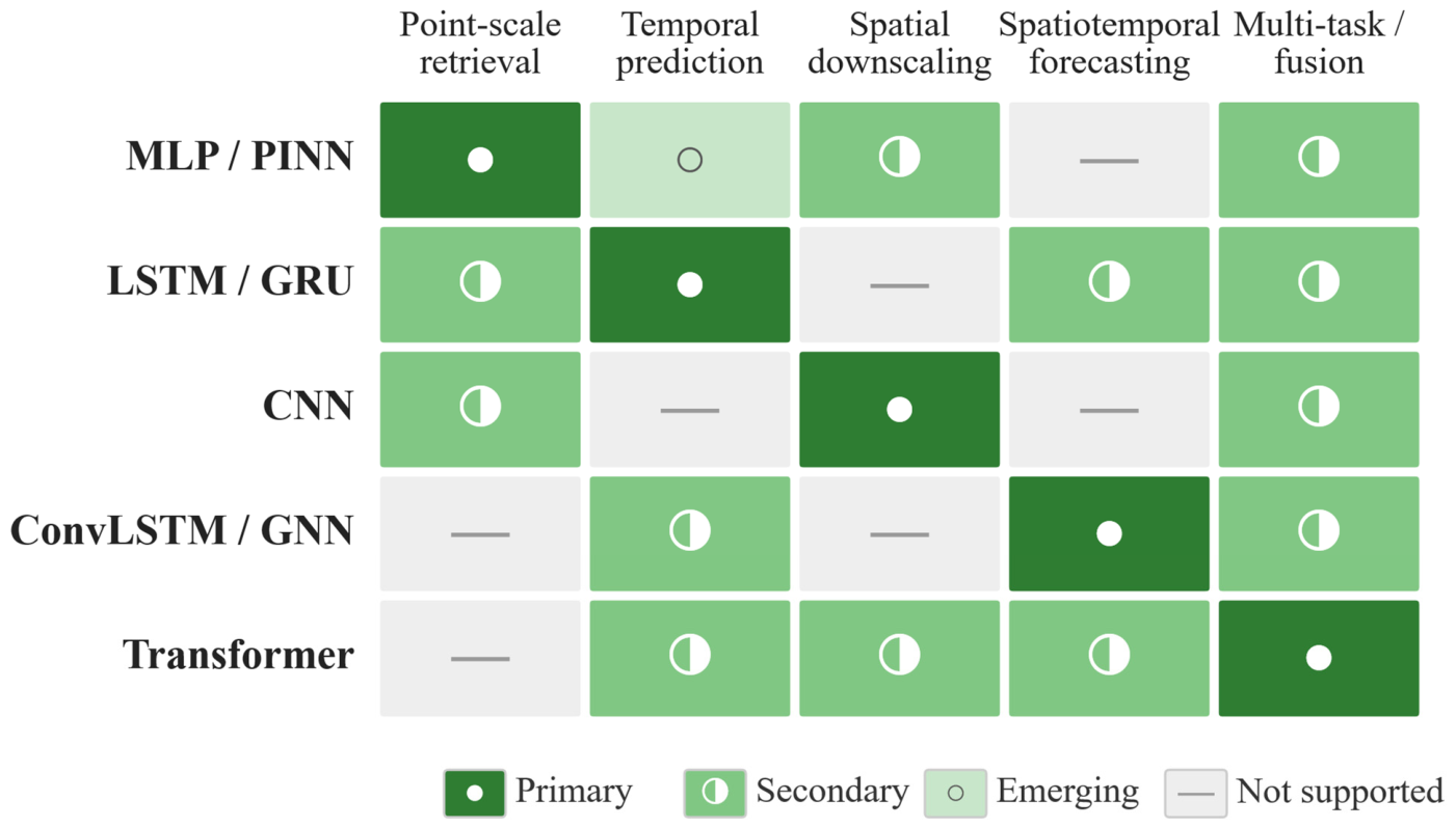
The survey in Section 3 reveals a consistent pattern: each deep learning architecture occupies a distinct niche defined by the target variable’s spatial and temporal structures, the dominant data source, and the physical complexity of the estimation problem (Table 2). MLP-based ANNs and PINNs are suited to point-scale surface SM retrieval tasks where the physics of microwave-soil and canopy interactions can be directly embedded. Figure 3 maps this architecture–task capability matrix across five principal task types.

LSTM and GRU architectures dominate temporal SM prediction across spatial scales: from CONUS-scale SMAP gap-filling and hindcasting [5,32,33] through multiscale satellite-in situ fusion at 9 km [34] and globally distributed field-scale retrieval [35]. Their common strength is gated memory, which captures the multi-day hydrological memory of soil moisture more effectively than non-recurrent architectures at comparable temporal resolutions. The two recurrent families differ in complexity and deployment trade-offs. LSTM uses separate input, forget, and output gates, together with an explicit cell state, making it well suited to longer or multi-timescale memory but generally increasing the parameter count and training/inference costs. GRU combines gating into a simpler recurrent unit, making it lighter and often more attractive when training data, compute budgets, or near-real-time latency is limiting. The practical choice is therefore task-dependent rather than a universal preference for one recurrent architecture.

ConvLSTM and GNN architectures address different spatial assumptions. ConvLSTM fills the spatiotemporal gap-filling niche for continuous gridded products at the SMAP revisit interval [50,54] because convolutional gates assume a regular grid and local neighborhood dependence. GNNs extend the same general goal to irregular sensor-network or graph-structured settings, where node-edge topology, heterogeneous connectivity, and nonlocal dependencies matter more than local convolution [56,57]. Hybrid graph-recurrent designs are therefore a natural direction when both temporal memory and irregular spatial dependence must be represented. Transformer networks are best suited to tasks with multi-source heterogeneity, very long sequences, or global scales, as demonstrated across climate projection, multi-decadal reconstruction, and high-resolution retrieval [59,60,61,62,63]. This architecture–task hierarchy enables evidence-based model selection for new SM estimation problems, reducing dependence on exhaustive trial-and-error benchmarking.

4.2. Physics-Guided Deep Learning

A unifying theme across all five architecture families is the consistent integration of physical knowledge, progressing from purely empirical data fitting through four distinct modes. Hard architectural constraints embed physical laws directly into the network structure, preventing physically inadmissible predictions [64,65]. Physics-as-input strategies embed physical models at the feature engineering stage, supplying physically meaningful inputs that pure satellite observables cannot provide [41,42,48,66]. Soft loss-function penalties add physical-consistency residuals as penalty terms alongside the data-fitting loss, training the network to honor physics without modifying its architecture [37,67]. Physics-ML hybrid output fusion averages independent physics-based and data-driven estimates, remaining the most operationally accessible mode [32,38].

The quantified benefits of physical integration are substantial and consistent across architecture families. At the parameter-sparse end, PIML-SM [30] achieved R = 0.94 and RMSE = 0.019 ${\mathrm{m}}^3\hspace{0.17em}{\mathrm{m}}^{-3}$ across 78 stations through physics-constrained training, and PLF-PINN [67] markedly reduced the sensitivity of loss-weight initialization and random seed variation in RRE-solving PINNs—both critical for practical deployment. For grid-scale SM estimation, PGDL-CNN-LSTM reduced physical inconsistency by 92% and cut the RMSE by 9.6% relative to an unconstrained CNN-LSTM, maintaining a correlation coefficient of 0.70 with only 50% of the training data [65]. For temporal SM prediction, physically guided LSTM loss functions improved KGE by 13.6% and R² by 20.7%, while reducing the RMSE by 8.2% globally [37].

4.3. Persistent Challenges

Despite substantial progress, three persistent performance constraints emerge across the reviewed literature. First, reported ubRMSE values remain strongly context-dependent. One low reported ubRMSE value is 0.022 ${\mathrm{m}}^3\hspace{0.17em}{\mathrm{m}}^{-3}$ for DI_ConvGRU over China [54], while many global or CONUS-wide products report values around 0.040–0.055 ${\mathrm{m}}^3\hspace{0.17em}{\mathrm{m}}^{-3}$ (Table 2). The SMAP mission accuracy target of ≤0.04 ${\mathrm{m}}^3\hspace{0.17em}{\mathrm{m}}^{-3}$ [1] is discussed here only for studies that explicitly report the ubRMSE; on that basis, the Wide-and-Deep CNN [44] reports 0.041 ${\mathrm{m}}^3\hspace{0.17em}{\mathrm{m}}^{-3}$, whereas the multiscale LSTM [34] is listed separately as a total-error reference because the ubRMSE was not reported. The Transformer-adjacent examples include ubRMSE = 0.043 ${\mathrm{m}}^3\hspace{0.17em}{\mathrm{m}}^{-3}$ [61]. These values indicate the order of magnitude achieved under specific validation settings, not a universal ordering of model families. Second, regarding dense vegetation opacity, the C-band SAR signal saturates above typical crop-canopy VWC thresholds, and passive L-band retrievals degrade when the vegetation water content exceeds approximately 5 kg m⁻² [47]; WCM preprocessing [41,42] and SMAP–ERA5 fusion [47] offer partial mitigation, as independently reported across LSTM [35], CNN [46], and Transformer [60] studies conducted under contrasting conditions, which is a consistent pattern seen across architecture families.

Third, regarding extreme SM events, one systematic regional comparison observed elevated errors when SM exceeded the 75th percentile of the SM distribution across four spatiotemporal architectures on the North China Plain [52], directly reflecting training data imbalance; whether this threshold generalizes across climate regimes and architectures remains untested. Physical constraints that bound outputs within residual-to-saturated limits [65] provide additional mitigation but remain insufficient for the full range of extreme events. Rigorous uncertainty quantification, beyond the isolated MC-dropout and SHAP explainability [40] applications reviewed here, is needed before DL SM products can be confidently assimilated into operational early drought or flood warning systems.

Computational and deployment constraints form a fourth practical challenge. MLP and shallow PIML models are relatively lightweight and suitable for small in situ datasets or fast retrieval. CNN downscaling introduces a moderate cost because memory and training time increase with spatial resolution and auxiliary-input stacks. LSTM and GRU models add sequence-length-dependent training costs, with GRU generally offering a lighter alternative when latency or the parameter count is limiting. ConvLSTM and GNN models are more demanding because they maintain spatial hidden states or graph-topology operations, while Transformer-based fusion is likely to impose the highest training burden for long sequences and global multi-source archives. Because most reviewed studies do not report the training time, GPU type, parameter count, or inference latency consistently, these computational costs can only be compared qualitatively here. For operational early drought or flood warnings, model selection therefore needs to consider not only the predictive skills but also the sequence length, parameter count, memory use, inference latency, data latency, hardware budget, and the reliability of near-real-time data pipelines.

Beyond predictive skill alone, non-linear complexity indicators such as permutation entropy, sample entropy, or multiscale entropy may provide complementary information for interpretable monitoring and early warnings. For example, Qin et al. [68] recently used a permutation-entropy-based framework to detect subtle transient fluctuations in monitored seawall settlement data, illustrating how entropy measures can support interpretable anomaly detection in water-related infrastructure monitoring. These measures are not part of the core DL application sample reviewed here, but they do offer useful cross-domain diagnostic ideas when the objective is not only point estimation but also detecting regime shifts, transient disorders, and changes in temporal organization.

This review also has several limitations. First, the scope is restricted to remote sensing-based surface SM; therefore, root-zone and deeper-profile estimations are treated only as adjacent future directions rather than as a systematic review target. Second, the evidence base is geographically uneven: successful demonstrations are concentrated in CONUS, China, Europe, and India, whereas Africa and South America remain underrepresented because of sparse in situ validation networks and limited benchmark datasets. Third, reported performance values are not always directly comparable because studies differ in depth, scale, temporal aggregation, validation networks, and whether the RMSE or ubRMSE is reported.

4.4. Ecohydrological Relevance and Future Directions

The connections drawn in this section represent demonstrated accuracy capabilities rather than deployed ecohydrological monitoring systems; translating these DL products into routine ecological forecasting remains an open integration challenge. Satellite-observed surface SM is directly relevant to vegetation water uptake: Feldman et al. [69] showed that grasslands and croplands—covering more than one-third of global vegetated surfaces—draw water predominantly from the upper soil layer, making them closely trackable by L-band SM observations. Konings et al. [70] demonstrated that anisohydric grassland productivity is strongly sensitive to vapor pressure deficits, which are tightly coupled to near-surface SM through land–atmosphere exchange. Therefore, improved DL-derived SM products directly strengthen ecosystem-scale evapotranspiration estimates. Humphrey et al. [71] further showed that SM variability drives the dominant fraction of interannual global land carbon uptake variability, making advances in SM retrieval accuracy consequential for constraining carbon cycle projections.

The operational value of accurate SM extends to agricultural drought monitoring and early flood warnings. Bolten et al. [72] demonstrated that assimilating satellite SM retrievals into a two-layer water balance model improved continental SM estimates and supported USDA crop yield monitoring, making SM accuracy directly consequential for food security assessments. Massari et al. [73] showed that H-SAF SM products reproduced 593 flood events across 35 Italian catchments with a median Nash–Sutcliffe efficiency of 0.64. DL architectures that deliver spatially continuous, near-real-time SM therefore directly strengthen these operational systems. The SoMo.ml 18-year continuous European SM dataset [36] provides the temporal continuity needed to resolve SM-driven controls on grassland productivity of the type that is documented by Konings et al. [70].

Two frontier research directions emerge from the ecohydrological requirements identified above and the performance ceilings detailed in Section 4.3. Dense vegetation opacity at C-band (Sentinel-1) and L-band SMAP wavelengths persistently degrades SM retrieval accuracy under forest canopies and high-biomass cropland, motivating the adoption of the upcoming NISAR L-band SAR mission (which employs deeper canopy penetration and broader temporal coverage) as the next-generation sensor for physics-informed DL frameworks that link surface moisture to plant water stress in structurally complex vegetation. Extending temporal and geographic generalizations beyond the SMAP training period, as well as CONUS and Europe, requires geospatial foundation model pre-training on diverse multi-sensor archives or stronger physical regularization. Integrating physics-embedded uncertainty quantification for operational data assimilation into these frameworks would complete the journey from DL-derived SM estimates to operational ecohydrological monitoring and prediction infrastructure.

Root-zone and deeper-profile soil moisture, including profiles extending toward 2 m, represents an adjacent but important future extension for ecohydrological applications because plant water uptake, agricultural drought, and land–atmosphere coupling are often controlled by moisture availability below the satellite sensing depth. Several adjacent studies indicate possible pathways for linking surface remote-sensing retrievals to deeper soil layers: SMAP Level-4 provides a surface and root-zone soil moisture product that is evaluated against in situ observations [10]; explainable transfer learning has been tested for subsurface SM prediction at 7–28 cm depth [40]; physics-constrained spatiotemporal DL has been extended to multi-layer grid-scale SM estimations [65]; Hydrus-1D simulations have been coupled with ConvLSTM for root-zone SM estimations [66]; and RRE/PINN-based studies show how soil–water physics can constrain vertical water-flow or profile estimations [64,67]. These studies are treated here as boundary cases rather than as a separate review corpus because the present review is focused on remote sensing-based surface soil moisture monitoring and prediction.

5. Conclusions

The reviewed evidence shows that deep learning has reshaped remote sensing-based SM estimation over the SMAP era (2015–2026), with the field advancing from isolated ANN applications to five architecture families (MLP/PINN, LSTM/GRU, CNN, ConvLSTM/GNN, and Transformer), each suited to a distinct combination of spatial scale, data modality, and physical complexity. Across all five families, embedding physical knowledge into the DL training process has become the dominant design strategy: physical constraints improve accuracy, reduce reliance on large training datasets, and make outputs physically consistent, outcomes that neither data-only nor physics-only approaches reliably deliver in combination. The examples below are interpreted within their original task and validation contexts, not as a formal cross-study leaderboard.

Three bodies of evidence support these conclusions. First, architecture–task matching is supported by context-specific performance reports: multi-source ANN retrieval achieves RMSE = 0.040 ${\mathrm{m}}^3\hspace{0.17em}{\mathrm{m}}^{-3}$ over topographically complex alluvial terrain, which is a useful total-error reference but not directly comparable to the SMAP ubRMSE target because ubRMSE was not separately reported; LSTM achieves RMSE < 0.035  ${\mathrm{m}}^3\hspace{0.17em}{\mathrm{m}}^{-3}$ for CONUS-wide SMAP temporal extension; DI_ConvGRU reaches ubRMSE = 0.022  ${\mathrm{m}}^3\hspace{0.17em}{\mathrm{m}}^{-3}$ for real-time spatiotemporal gap-filling over China; CNN-based Wide-and-Deep learning reports ubRMSE = 0.041  ${\mathrm{m}}^3\hspace{0.17em}{\mathrm{m}}^{-3}$ at 1 km over CONUS; and TSMSNet extends SM estimation to 2099 under three CMIP6 SSP scenarios at global scale. Second, physics-DL integration consistently improves accuracy across all five architecture families, with relative RMSE improvements ranging from −8.2% for PHYS-LSTM to −50% for PIML-SM relative to a data-driven ANN baseline; in the most rigorously controlled ablation, the physics-regularized spatiotemporal model additionally reduced physical inconsistency by 92% and maintained accuracy with only half the training observations. Third, multi-source satellite fusion (combining SMAP L3/L4, Sentinel-1/2, ERA5-Land, and in situ ISMN/SCAN/USCRN observations) is the convergent input paradigm across all architectures, enabling surface SM products spanning three spatial-temporal scales: 1 km daily fields over CONUS [44], globally applicable ≈ 320 m retrievals [63], and 72-year historical reconstruction over the Yellow River Basin [61].

Taken together, these results show that DL-based tools are increasingly capable of delivering ecohydrologically meaningful SM information for vegetation water-stress monitoring, early agricultural drought warning, early flood warning, and land–atmosphere coupling quantification. This information is becoming spatially explicit at sub-kilometer resolutions, temporally continuous across multi-decadal periods, and physically consistent. These capabilities position DL-based SM estimation as a promising layer for ecohydrological modeling, linking satellite-observed surface moisture to evapotranspiration partitioning, water-mediated biogeochemical cycles, and the resilience of terrestrial and aquatic ecosystems under climate variability and anthropogenic pressures.

Resolving the two core surface SM challenges identified—vegetation-penetrating SM retrieval via NISAR and temporal-geographic generalization via foundation model pre-training, together with physics-embedded uncertainty quantification for operational data assimilation—would help transform DL-based SM estimation from a research capability into operational ecohydrological monitoring infrastructure. Root-zone and deeper-profile predictions toward 2 m should be treated as adjacent extensions that can build on these surface SM advances through data assimilation, transfer learning, and physics-guided vertical constraints.