Evolution of Hydraulic Conductivity and Identification of Apparent Seepage-Transition Hydraulic Gradients in Graded Sandy Soils Under Staged Upward Seepage

Abstract

Staged upward seepage can trigger particle migration and pore-structure adjustment in graded sandy soils, but the resulting transition behavior remains difficult to identify quantitatively. In this study, three representative sandy soils from a deep overburden deposit in southeastern Tibet were tested using a laboratory vertical upward seepage apparatus. Eight specimens with different nominal preparation states were subjected to stepwise increases in hydraulic head difference. Local hydraulic gradient, seepage velocity, hydraulic conductivity, and macroscopic outflow phenomena were monitored. Apparent seepage-transition hydraulic gradients were identified by combining abrupt changes in k–i curves, conductivity ratios between eligible staged records, and observed seepage responses. The clearest transition occurred in the nominal loose specimen of Soil 2, where the temperature-corrected hydraulic conductivity k₂₀ increased from 1.76 × 10⁻³ to 2.25 × 10⁻² cm s⁻¹ as i increased from 0.20 to 0.25, giving k_20,2/k_20,1 = 12.80 and i_c = 0.225. A clear transition was also identified for the nominal dense specimen of Soil 3, with k_20,2/k_20,1 = 6.61 and i_c = 0.583. Clear transitions were identified in the tested specimens only for Groups D and H, whereas the remaining specimens showed weak or phenomenon-assisted responses, local high-gradient fluctuations, or anomalous loading-path records rather than uniformly identifiable transition points. These results show that apparent transition gradients are path-dependent and should be evaluated together with loading history, seepage-velocity evolution, conductivity ratios, and macroscopic observations.

1. Introduction

Changes in groundwater seepage conditions are an important factor inducing seepage-stability problems in granular soils. In embankments, dam-foundation overburden layers, foundation-pit dewatering zones, and deep overburden deposits in high-mountain valleys, water-level fluctuation, increased local head difference, and upward seepage can modify the internal hydraulic-gradient distribution of soil masses. As the hydraulic gradient increases, fine particles may migrate, be lost, or rearrange under seepage forces, leading to pore-structure adjustment and the formation of preferential seepage channels. These processes can further increase hydraulic conductivity and reduce seepage stability. Therefore, identifying seepage-state transitions in graded sandy soils from the perspective of seepage-parameter evolution is important for evaluating the seepage stability of overburden layers, embankments, and dam foundations [1,2,3,4].

Previous studies have shown that internal erosion, suffusion, and piping in granular soils are jointly controlled by gradation, fines content, density state, stress state, and hydraulic loading path. Classical internal-stability criteria generally evaluate whether fine particles can migrate through the pore channels of a coarse-particle skeleton on the basis of particle-size distribution and pore-channel conditions [5,6,7,8,9,10,11]. Seepage tests have further demonstrated that changes in hydraulic conductivity, eroded-particle mass, and local pore structure during increasing hydraulic gradients can reflect the development stages of internal erosion [12,13,14,15,16]. In recent years, fine-particle migration and changes in critical hydraulic gradient under upward seepage, cyclic hydraulic loading, horizontal seepage, and rainfall infiltration have also received increasing attention [17,18,19,20,21]. These studies provide a basis for understanding the seepage evolution of graded sandy soils under hydraulic loading. However, the evolution of k–i curves, identification of apparent transitions, and influence of the loading path under staged upward seepage remain insufficiently discussed.

Based on these considerations, three representative graded sandy soils collected from a deep overburden deposit in a high-mountain valley in southeastern Tibet were tested using laboratory vertical upward seepage experiments under staged hydraulic loading. The objective of this study was not to determine a universal theoretical critical hydraulic gradient but to identify apparent seepage-state transitions under specific experimental boundaries and loading paths. The specific aims were to: (1) examine the evolution of seepage velocity and hydraulic conductivity for soils with different gradations and nominal preparation states; (2) develop an identification approach based on abrupt changes in k–i curves, conductivity ratios between eligible staged records, and macroscopic outflow observations; and (3) evaluate the effects of non-monotonic loading, post-disturbance seepage, and experimental boundary conditions on the identified transition values. The apparent seepage-transition hydraulic gradient defined here differs from the classical critical hydraulic gradient for global hydraulic heave and from initiation gradients determined using direct evidence of suffusion. It is an operational, specimen- and loading-path-dependent indicator inferred from discrete changes in local hydraulic response; it does not represent a unique force-balance threshold or a direct measurement of the onset of particle loss.

2. Materials and Methods

2.1. Test Materials and Gradation

The test soils were collected from a deep overburden deposit in a high-mountain valley in southeastern Tibet. The field overburden deposit is thick and shows pronounced differences in particle composition, with sand, gravel, and a small amount of fines. Pore-structure adjustment may occur under seepage action. Sieve analysis, grain-size distribution curve plotting, and gradation-index calculation were conducted with reference to the Standard for Geotechnical Testing Method [22]. Based on field investigation data and sieve-analysis results, three representative graded soils were reconstituted and denoted as Soil 1, Soil 2, and Soil 3.

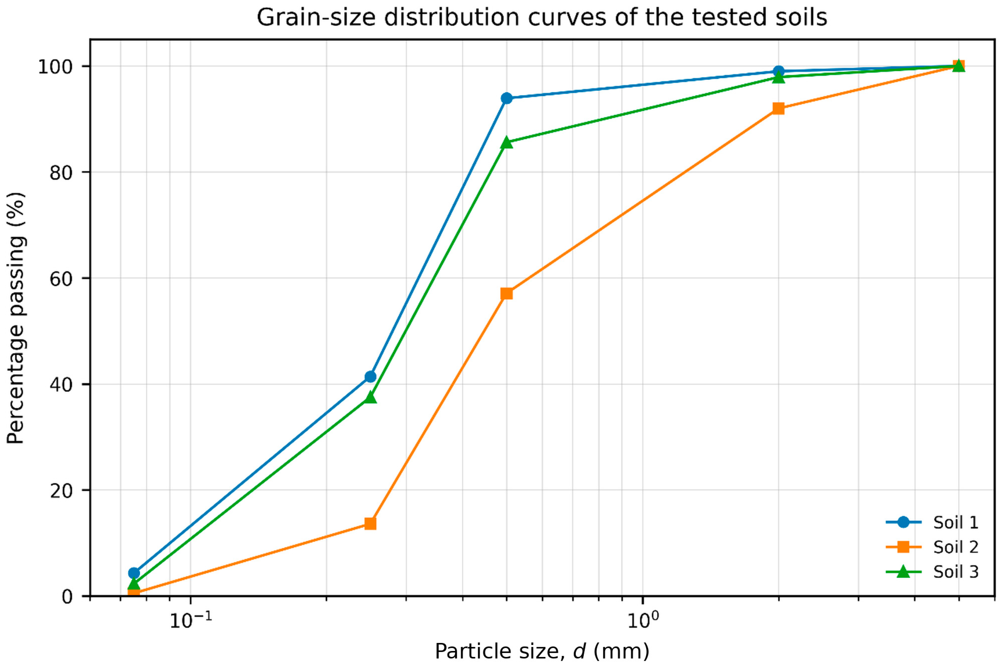
Figure 1 shows that the gradation curve of Soil 2 is generally lower than those of Soils 1 and 3, and its d₁₀, d₃₀, and d₆₀ values are all larger, indicating that Soil 2 is coarser overall. Soils 1 and 3 have higher percentages passing in the small-particle-size range. The proportion of particles smaller than 0.25 mm is 41.4% and 37.5%, respectively, which are much higher than the 13.6% of Soil 2. The fines contents, calculated as particles smaller than 0.075 mm, are 4.3%, 0.5%, and 2.3%, respectively. The characteristic particle sizes and gradation indices of the three soils are listed in

Table 1. Particle-size indices of the tested soils.

Soil ID	d10/mm	d30/mm	d60/mm	Cu	Cc	Fines Content (%)
Soil 1	0.0902	0.1727	0.3196	3.54	1.03	4.3
Soil 2	0.1796	0.3247	0.5610	3.12	1.05	0.5
Soil 3	0.0976	0.1934	0.3457	3.54	1.11	2.3

.

2.2. Test Groups and Specimen Preparation

Eight groups of specimens were prepared based on the three soil gradations. For Soil 1, three nominal preparation states were prepared and denoted as Groups A, B, and C, respectively. Group A was prepared under a nominal loose condition, Group B under a nominal in situ-density condition, and Group C under a nominal higher-density condition. For Soil 2, because of the relatively high proportion of coarse particles, the target nominal higher-density condition was difficult to prepare repeatedly and stably under the current permeameter size and layered filling conditions. Therefore, only nominal loose and nominal in situ-density conditions were prepared and denoted as Groups D and E. For Soil 3, nominal loose, nominal in situ-density, and nominal dense conditions were prepared and denoted as Groups F, G, and H. Because the void ratio and relative density were not further measured at this stage, the nominal preparation state was mainly determined from the specimen mass and volume. Future work should combine the void ratio, relative density, and repeated tests to further quantify the effect of nominal preparation state on the apparent seepage-transition hydraulic gradient. The basic parameters of each group are listed in

Table 2. Test groups and basic parameters.

Soil ID	Group	Nominal Preparation State	Specimen Mass (g)	Specimen Length (cm)	Nominal Preparation Density, ρ (g cm−3)
Soil 1	A	Nominal loose	1600	21.5	1.481
Soil 1	B	Nominal in situ density	1647	21.0	1.561
Soil 1	C	Nominal higher density	1900	21.5	1.759
Soil 2	D	Nominal loose	1600	21.0	1.517
Soil 2	E	Nominal in situ density	1836	21.5	1.700
Soil 3	F	Nominal loose	1600	21.5	1.481
Soil 3	G	Nominal in situ density	1584	21.0	1.501
Soil 3	H	Nominal dense	1800	20.0	1.791

. The terms “nominal loose”, “nominal in situ density”, “nominal higher density”, and “nominal dense” were used to describe the preparation conditions controlled by specimen mass, specimen volume, layered filling, and compaction effort. Because the maximum and minimum dry densities were not determined using an independent standard procedure, and because the void ratio and relative density were not measured, these terms should not be interpreted as rigorously defined relative-density states. During specimen preparation, each particle-size fraction was weighed according to the designed gradation and thoroughly mixed. The mixed soil was then placed into the permeameter by layered filling. Loose specimens were prepared mainly by natural filling and slight leveling. Nominal in situ-density specimens were prepared by controlling specimen mass, layer thickness, and slight compaction, whereas nominal dense specimens were compacted appropriately during layered filling. The filling thickness and treatment method of each layer were kept consistent, and local concentration of coarse particles and preferential flow along the cylinder wall were avoided as much as possible. After specimen placement, water was introduced slowly for saturation. The formal test began after continuous outflow and stable flow rate were achieved.

2.3. Seepage Apparatus and Test Procedure

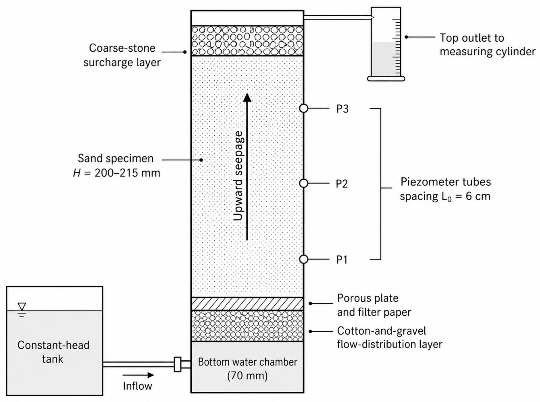
A custom-fabricated acrylic vertical seepage apparatus, fabricated by Xi’an Shuanghang Advertising Co., Ltd. (Xi’an, China), was used, as shown schematically in Figure 2. The inner diameter of the permeameter was D = 80 mm. Taking π = 3.14, the effective specimen cross-sectional area was A = 50.24 cm². The wall thickness was approximately 10 mm. The specimen height was determined according to specimen mass and nominal preparation state and ranged from 200 to 215 mm. The top of the permeameter was open, and the upper side outlet was connected to a measuring cylinder to collect and measure the outflow. During testing, a coarse-gravel surcharge layer was placed above the specimen to reduce surface disturbance caused by upward seepage.

The bottom of the permeameter was connected to a 70 mm high water-storage chamber. A filter-cotton and gravel flow-distribution layer was placed in the chamber. Water flowed from a constant-head tank into the bottom chamber and then entered the permeameter from bottom to top after being dispersed by the distribution layer. A porous plate and filter paper were placed at the bottom of the specimen to improve inflow uniformity and prevent particles from entering the bottom pipeline. The vertical seepage apparatus and staged loading method were designed with reference to constant-head permeability tests and internal erosion tests [14,15,23]. Because the permeameter used a rigid acrylic wall and no flexible membrane or perimeter sealing system was installed, possible wall effects could not be completely eliminated. In particular, preferential seepage may develop along the soil–wall interface in loose specimens or after local particle rearrangement. Such preferential seepage could increase the measured outflow at a given local head difference and may therefore lead to underestimation of the apparent transition gradient, although the magnitude of this effect could not be quantified with the present apparatus. During specimen preparation and saturation, layered filling, slow water introduction, and a coarse-gravel surcharge layer were used to reduce local disturbance and side-wall flow as much as possible. Nevertheless, the measured hydraulic gradients and apparent transition values should be interpreted as apparatus-dependent values under the present boundary conditions.

Three 10 mm diameter piezometer taps, denoted as P1, P2, and P3 from bottom to top, were installed along the side wall of the permeameter. The upper surface of the bottom flange plate coincided with the bottom of the specimen. The lower edges of P1, P2, and P3 were located 50, 110, and 170 mm above the bottom of the specimen, corresponding to center elevations of 55, 115, and 175 mm, respectively. The center-to-center distance between adjacent taps was therefore L₀ = 60 mm. Because the specimen height ranged from 200 to 215 mm, the center of P3 was located 25–40 mm below the specimen free surface. During testing, P3 was used only for an on-site qualitative comparison of the head differences over the upper interval (P2–P3) and the lower interval (P1–P2). No obvious difference between the two intervals was noted on site; however, the P3 readings were not included in the formal dataset, and no quantitative comparison between the two intervals is reported. Therefore, the local hydraulic gradient reported in this study was calculated only from the systematically retained P1–P2 head difference, rather than from P2–P3 or from the total head loss over the full specimen height. The P1–P2 interval was selected to reduce the influence of potentially non-uniform head losses near the bottom porous plate, filter layer, surcharge layer, and free surface, thereby providing a more direct representation of the seepage response within the monitored local section. Therefore, the reported i_c values represent local apparent transition gradients rather than average gradients over the full specimen height. The other i_rep values likewise refer to the monitored P1–P2 section but should be interpreted according to their respective qualitative, fluctuating, or non-monotonic classifications. Before the formal test, water was introduced slowly to fully saturate the specimen and to remove air bubbles from the pipeline and specimen as much as possible. After continuous outflow and stable piezometer readings were obtained, the head difference was increased stepwise.

The formal test was conducted by gradually increasing the head difference. A fixed holding time or fixed outflow-measurement duration was not prescribed for each head level because the seepage rate differed substantially among specimens and loading stages. At each head level, the specimen was allowed to approach a stable seepage condition, indicated by no obvious fluctuation in the piezometer readings. The outflow was then measured twice on site over a suitable time interval selected according to the prevailing flow rate. A head level was accepted for formal recording when the relative difference between the two calculated outflow rates (Q/t) was less than 5% and the piezometer readings remained stable. The first measurement was retained as the representative record for calculating v and k. The second measurement was used only for the on-site stability check and was not systematically retained; therefore, a stage-by-stage statistical repeatability analysis was not performed. The head difference between P1 and P2 (Δh), measurement time (t), outflow volume (Q), and observed phenomena corresponding to the retained record were then recorded.

2.4. Calculation of Seepage Parameters and Identification of the Apparent Seepage-Transition Hydraulic Gradient

Based on the stable-stage records obtained following the procedure described in Section 2.3, the test records included the head difference between P1 and P2 (Δh), measurement time (t), outflow volume (Q), and specimen length (L). The specimen length L was used only for density calculation and was not used in the calculation of hydraulic gradient or hydraulic conductivity. The seepage-parameter calculation was based on Darcy seepage theory [24]. Water temperature was recorded for the formal records of Groups B–H. During data checking, the water temperature of record E12 was noted in the authors’ laboratory record and added to the dataset. For records with available water-temperature measurements, the hydraulic conductivity calculated under the measured water-temperature condition was corrected to the standard value at 20 °C using the viscosity correction k₂₀ = k_T × (μ_T/μ₂₀), where k_T is the hydraulic conductivity at the measured water temperature T, μ_T is the dynamic viscosity of water at temperature T, and μ₂₀ is the dynamic viscosity of water at 20 °C. The dynamic viscosity of water was calculated as μ(T) = 2.414 × 10⁻⁵ × 10^{247.8/(T+133.15)} Pa·s, where T is the recorded water temperature in °C. The temperature-correction factor was then calculated as μ_T/μ₂₀ [25]. Because water-temperature records were not available for Group A, its hydraulic-conductivity values were retained as measured values and used only for qualitative, phenomenon-assisted interpretation rather than temperature-standardized quantitative ranking. The apparent seepage-transition hydraulic gradient was identified by combining abrupt changes in hydraulic conductivity, local hydraulic-gradient variation, and macroscopic outflow phenomena [13,14,15,16].

The main parameters were calculated using Equations (1)–(3):

$$i={\displaystyle \frac{\Delta h}{L_0}}$$

(1)

$$v={\displaystyle \frac{Q}{At}}$$

(2)

$$k={\displaystyle \frac{v}{i}}={\displaystyle \frac{Q{L}_0}{At\Delta h}}$$

(3)

where i is the local hydraulic gradient; v is the seepage velocity in cm s⁻¹; k is the hydraulic conductivity in cm s⁻¹; Q is the outflow volume in cm³; A is the effective specimen cross-sectional area, taken as 50.24 cm² in this test; t is the measurement time in s; Δh is the head difference between P1 and P2 in cm; and L₀ is the center-to-center distance between P1 and P2, taken as 6 cm in this test.

The apparent seepage-transition hydraulic gradient in this study refers to the seepage-state transition point indicated jointly by abrupt changes in hydraulic conductivity, changes in seepage velocity, and macroscopic outflow phenomena under the staged upward seepage loading path used in this test. This value reflects the apparent response associated with pore-structure adjustment, fine-particle migration, or preferential seepage-channel development under specific experimental boundaries and loading paths. It is not equivalent to a unique theoretical critical hydraulic gradient corresponding to particle suspension, global heave, or complete seepage failure.

When hydraulic conductivity changed from a relatively stable or slightly fluctuating state to a pronounced increase between two adjacent eligible hydraulic-gradient records after excluding records marked as non-monotonic or post-disturbance, and when the subsequent seepage velocity continued to increase or was accompanied by outflow turbidity, fine-particle discharge, or specimen-surface disturbance, the interval was identified as a seepage-state transition interval. To reduce subjective judgment, the conductivity ratio between such eligible staged records, k₂/k₁, was further used as an auxiliary criterion. For temperature-corrected records, this ratio was calculated as k_20,2/k_20,1, whereas for Group A, it was calculated using the measured hydraulic conductivity because water-temperature records were not available. It should be noted that the conductivity-ratio thresholds of 2.0 and 1.5 were not intended as universal theoretical criteria. They were adopted as empirical classification thresholds for the present staged-loading dataset. A conductivity ratio of 2.0 or greater indicates that the hydraulic conductivity at the subsequent eligible record at least doubled. When the ratio was ≥2.0 and the subsequent seepage velocity continued to increase or an obvious macroscopic phenomenon was observed, the transition was regarded as relatively clear. When 1.5 ≤ k₂/k₁ < 2.0, the response was classified as a weak transition only when it was supported by the subsequent seepage trend and/or a clear macroscopic observation; otherwise, it was treated as an unconfirmed weak response. When k₂/k₁ < 1.5 and no clear outflow turbidity, particle discharge, specimen failure, or sustained seepage-velocity increase was observed, the response was described as a local fluctuation rather than a confirmed transition. When k₂/k₁ < 1.5 but a clear macroscopic failure or disturbance was observed, the response was retained only as phenomenon-assisted qualitative evidence. Abrupt increases occurring during the first or second loading stage were not used independently as evidence of a seepage-state transition unless they were followed by sustained increases in hydraulic conductivity and seepage velocity or were accompanied by clear macroscopic phenomena, because these early-stage changes may reflect initial stabilization, residual-air removal, or local seating adjustment. Because these empirical classifications depend on the hydraulic-gradient increment and measurement resolution, the same specimen could be assigned differently under a finer or coarser loading schedule. No analytical or statistical calibration of the thresholds was performed; they are used only as descriptive rules for the present dataset. For monotonic intervals that satisfied the clear- or weak-transition criteria, the apparent seepage-transition hydraulic gradient was estimated as follows:

$$i_c={\displaystyle \frac{i_1+i_2}{2}}$$

(4)

where i₁ and i₂ are the local hydraulic gradients before and after the transition, respectively. For presentation in

Table 3. Representative hydraulic-gradient levels, conductivity ratios, and response classifications.

Soil ID	Group	Nominal Preparation State	ρ (g cm−3)	i1	i2	irep	Conductivity Ratio	Classification
Soil 1	A	Nominal loose	1.481	0.6667	0.8500	0.758	1.225 †	Phenomenon-assisted/qualitative only
Soil 1	B	Nominal in situ density	1.561	0.6667	0.7833	0.725	1.638	Weak transition
Soil 1	C	Nominal higher density	1.759	0.9333	1.0000	0.967	1.471	High-gradient fluctuation/weak response
Soil 2	D	Nominal loose	1.517	0.2000	0.2500	0.225	12.803	Clear transition
Soil 2	E	Nominal in situ density	1.700	1.3833	1.4000	1.392	1.324	High-gradient fluctuation
Soil 3	F	Nominal loose	1.481	1.0333	0.8167	0.925 *	9.724	Anomalous loading path
Soil 3	G	Nominal in situ density	1.501	1.3167	0.4500	0.883 *	16.094	Anomalous loading path
Soil 3	H	Nominal dense	1.791	0.4500	0.7167	0.583	6.605	Clear transition

Notes: For Groups B–H, the conductivity ratios were calculated using temperature-corrected hydraulic conductivity k₂₀. For Group A, water-temperature records were unavailable; the ratio marked by † was calculated using the measured hydraulic conductivity, and Group A was used only for qualitative, phenomenon-assisted interpretation. The E12 water-temperature entry was noted from the authors’ laboratory record. The value i_rep is the arithmetic midpoint of the listed point pair. For Groups B, D, and H, i_rep corresponds to i_c. For Groups A, C, and E, it is only a representative hydraulic-gradient level consistent with the classification in the final column. For Groups F and G, the values marked by an asterisk are i_m, the arithmetic midpoints of non-monotonic pairs with i₂ < i₁; they are not i_c values and are excluded from the monotonic ranking. Classification criteria: A conductivity ratio ≥ 2.0 was classified as a clear transition when supported by the subsequent seepage response or a clear macroscopic observation. A ratio satisfying 1.5 ≤ k₂/k₁ < 2.0 was classified as a weak transition only when supported by the subsequent trend and/or a clear macroscopic observation; otherwise, it was treated as an unconfirmed weak response. A ratio < 1.5 without supporting macroscopic evidence was treated as a local fluctuation, whereas a ratio < 1.5 accompanied by a clear failure phenomenon was retained only for phenomenon-assisted qualitative interpretation. Non-monotonic records were classified separately. For Group B, visible specimen failure was noted in the authors’ laboratory record at the second stage of the identified interval; this observation was used only as qualitative macroscopic supporting evidence for the weak-transition classification.

, i_rep denotes the arithmetic midpoint associated with each listed point pair. For monotonic intervals classified as clear or weak transitions, i_rep is interpreted as i_c = (i₁ + i₂)/2. For phenomenon-assisted, fluctuating, or unconfirmed monotonic responses, i_rep is only a representative hydraulic-gradient level and should not be interpreted as a confirmed i_c. For non-monotonic pairs with i₂ < i₁, i_rep = i_m = (i₁ + i₂)/2 is retained only as a descriptive midpoint and is not used in the monotonic ranking. The resolution-related half-width Δi_c = (i₂ − i₁)/2 applies only to monotonic transition intervals. Because only discrete staged records are available, segmented regression or exact change-point estimation was not performed. Figure 1, Figure 3, Figure 4 and Figure 5 were prepared using MATLAB R2025b (The MathWorks, Inc., Natick, MA, USA).

3. Results

3.1. Implications of Gradation Characteristics for Pore Structure

Table 1 shows that the coefficients of uniformity C_u of the three soils range from 3.12 to 3.54 and the coefficients of curvature C_c range from 1.03 to 1.11, indicating relatively continuous gradation within the dominant particle-size range. However, the particle proportions in different size ranges differ markedly. Soil 2 has the largest d₁₀, d₃₀, and d₆₀ values, suggesting a more pronounced coarse-particle framework. Soils 1 and 3 contain more particles smaller than 0.25 mm, which may increase the possibility of fine-particle filling within pore spaces. Their seepage process is therefore more susceptible to fine-particle migration and pore-channel reorganization. Previous studies have also shown that hydraulic conductivity and seepage-deformation behavior in sandy or coarse-grained soils are affected by effective particle size, void ratio, stress state, and internal erosion processes [5,9,10,11,26,27,28]. Accordingly, Soil 2 in the nominal loose state may have relatively stronger pore connectivity and may be more prone to preferential seepage-path development under enhanced hydraulic action, whereas Soils 1 and 3 may be more susceptible to fine-particle rearrangement, local migration, and pore-structure reorganization.

3.2. Seepage Velocity–Hydraulic Gradient Relationships

During the staged increase in hydraulic gradient, the seepage velocity–hydraulic gradient relationship can reflect the response of seepage velocity to hydraulic-gradient variation. If the pore structure of the specimen remains basically stable, seepage velocity changes continuously with increasing hydraulic gradient, and the conventional v–i curve is approximately linear or gently curved. After possible local fine-particle migration, pore-channel expansion, or preferential seepage-channel development, seepage velocity increases markedly and the curve slope may also change.

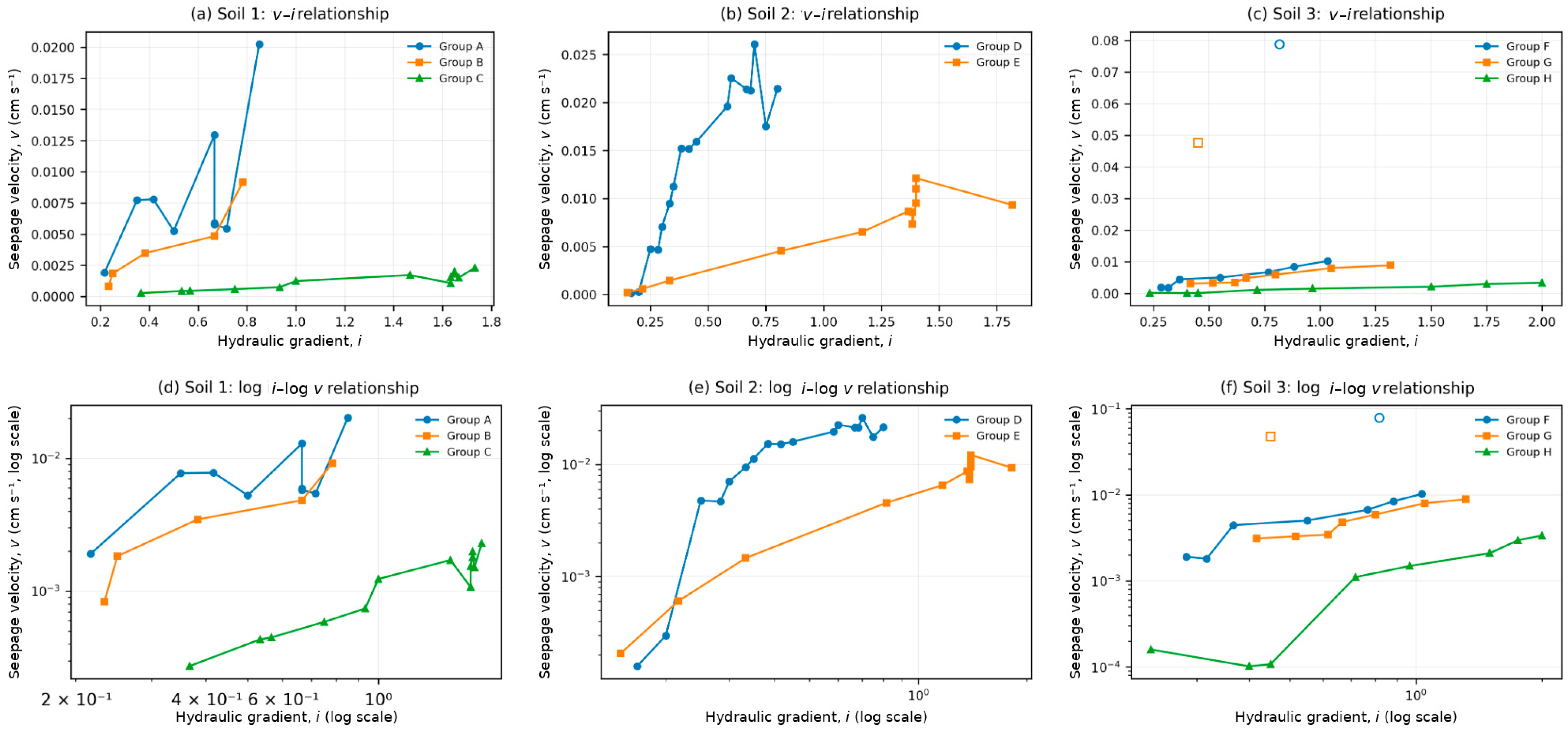
As shown in Figure 3, the three soils exhibited different seepage velocity–hydraulic gradient relationships under staged upward seepage. For Soil 1, Groups A and B changed relatively gently at low hydraulic gradients, and their seepage velocities increased more obviously in the later stage. Group C had a higher nominal preparation density and a lower overall seepage velocity; however, only a local high-gradient fluctuation or weak seepage response was observed near the high-gradient range. For Soil 2, Group D showed the most pronounced increase in seepage velocity at a relatively low hydraulic-gradient range. This response is consistent with a rapid increase in seepage velocity in the loose coarse-particle skeleton, possibly related to local pore-channel adjustment. Group E was prepared at a higher nominal density and showed a gentler overall response, with only local fluctuations at high hydraulic gradients. For Soil 3, Groups F and G showed high seepage-velocity points in the later stage, but these final points were associated with non-monotonic loading or post-disturbance seepage and were therefore plotted as isolated open markers rather than connected to the normal staged-loading curves. Group H had a low initial seepage velocity but still showed a pronounced increase in the later stage, suggesting that local pore-structure adjustment may also occur in the nominal dense specimen.

Overall, the v–i curves and the log i–log v plots can reflect staged changes in seepage velocity with increasing hydraulic gradient, but identifying transition points from these velocity-based curves alone remains partly subjective. Therefore, k–i curve changes, conductivity ratios between eligible staged records, loading-path characteristics, and macroscopic test phenomena were further combined for comprehensive judgment.

3.3. Evolution of k–i Curves

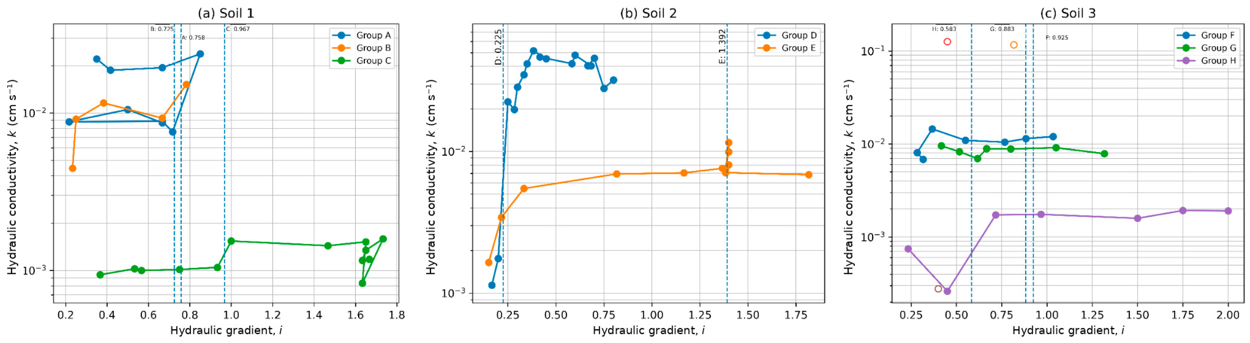
Compared with the seepage velocity–hydraulic gradient relationships, the k–i curve more directly reflects changes in hydraulic response that may be associated with internal structural adjustment. Figure 4 shows that the specimens generally experienced a relatively stable stage, a local fluctuation stage, and, for some groups, a sudden-increase stage. The relatively stable stage is consistent with the absence of obvious hydraulic evidence for structural adjustment. Local fluctuations may be related to fine-particle rearrangement or local pore-channel adjustment. A sudden-increase stage may indicate pore-structure adjustment, preferential seepage-path development, or intensified particle migration, but this interpretation remains qualitative because eroded-particle mass, turbidity, and post-test grain-size distributions were not continuously quantified.

For Soil 1, Group C showed an overall low hydraulic conductivity under the nominal higher-density preparation condition. After temperature correction, k₂₀ increased from approximately 1.05 × 10⁻³ to 1.54 × 10⁻³ cm s⁻¹ as i increased from 0.9333 to 1.0000, giving k_20,2/k_20,1 = 1.471. This response indicates a local high-gradient fluctuation or weak seepage response, but it does not satisfy the k_20,2/k_20,1 ≥ 1.5 threshold adopted in this study for a weak transition. For Soil 2, Group D showed the most pronounced abrupt change. When i increased from 0.20 to 0.25, k₂₀ increased sharply from 1.76 × 10⁻³ to 2.25 × 10⁻² cm s⁻¹, an increase of more than one order of magnitude. This response is consistent with possible local pore-channel adjustment or preferential seepage-path development in the loose coarse-particle specimen at a relatively low hydraulic gradient. Group E showed only local high-gradient fluctuations after temperature correction, and no confirmed transition was identified. For Soil 3, Groups F and G showed high k₂₀-value points, but these points were affected by non-monotonic loading or post-disturbance seepage. Group H showed a pronounced increase from 2.61 × 10⁻⁴ to 1.73 × 10⁻³ cm s⁻¹ between i = 0.4500 and 0.7167.

These results show that a low initial hydraulic conductivity does not necessarily correspond to a high apparent seepage-transition hydraulic gradient. Under the present preparation procedure, specimens with higher nominal preparation density generally showed lower hydraulic conductivity. However, local fine-particle redistribution or pore-channel adjustment may still cause a marked change in the k–i curve under increasing hydraulic gradient.

Representative post-test photographs are provided in Figure S1 as qualitative macroscopic evidence of local disturbance after seepage loading. These photographs were not used as quantitative measurements of internal particle migration.

3.4. Identification of Apparent Seepage-Transition Hydraulic Gradients

The raw staged-loading data for all specimen groups, including Δh, Q, t, i, v, k, water temperature, observed phenomena, and loading-path notes, are provided in Supplementary Table S1. According to the identification method proposed in Section 2.4, Table 3 lists the hydraulic-gradient point pairs before and after the identified conductivity changes, the representative hydraulic-gradient levels i_rep, the corresponding conductivity ratios, and the response classifications. For Group H, the record at i = 0.400 was classified as a non-monotonic/post-disturbance record and excluded from transition identification. The nearest eligible stages in the retained loading sequence, i = 0.450 and 0.7167, were then used, yielding i_c = 0.583 and k_20,2/k_20,1 = 6.61.

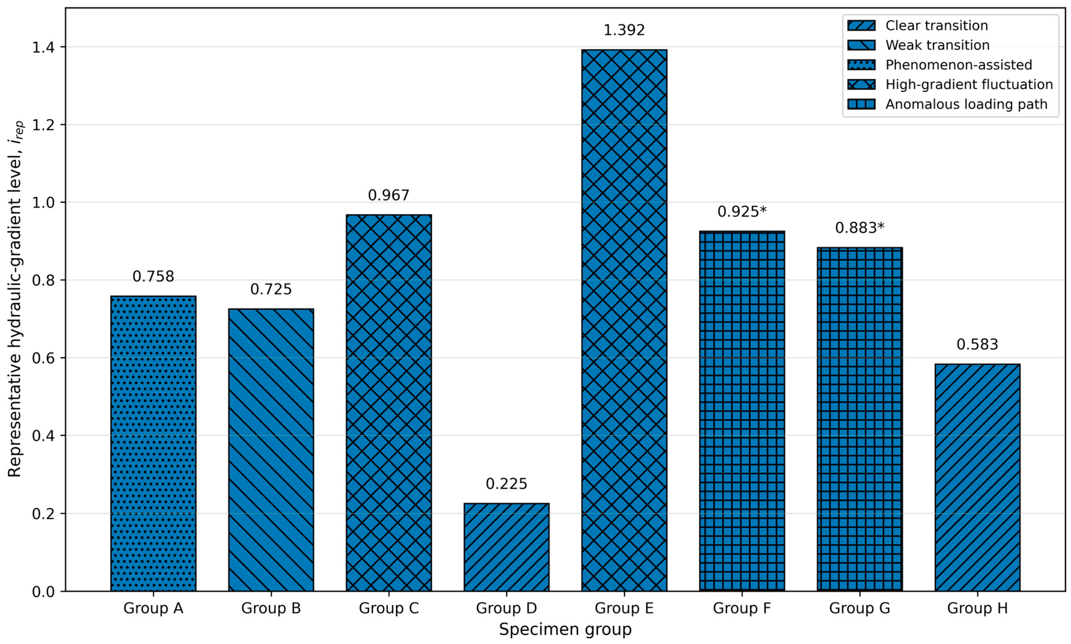
Table 3 and Figure 5 show that the magnitude and classification of the identified k–i responses differed markedly among the specimens. Group D of Soil 2 had the clearest seepage-state transition. When the hydraulic gradient increased from 0.20 to 0.25, the temperature-corrected hydraulic conductivity k₂₀ increased from 1.76 × 10⁻³ to 2.25 × 10⁻² cm s⁻¹, and k_20,2/k_20,1 reached 12.80, corresponding to i_c = 0.225. This response is consistent with possible local pore-channel adjustment or preferential seepage-path development in a loose coarse-particle skeleton at a relatively low hydraulic gradient. After excluding the H3 non-monotonic/post-disturbance record, Group H of Soil 3 showed a pronounced increase in hydraulic conductivity between the nearest eligible normal retained records at i = 0.4500 and 0.7167, with k_20,2/k_20,1 = 6.61 and i_c = 0.583, also indicating a relatively clear seepage-state transition.

In contrast, Group B of Soil 1 had k_20,2/k_20,1 = 1.638, which falls within the empirical range adopted for a weak transition. Visible specimen failure was noted in the authors’ laboratory record at the second stage of the identified interval and was used only as qualitative macroscopic supporting evidence. Therefore, this response was classified as a weak transition based mainly on the hydraulic-conductivity change, with macroscopic observation used as supporting evidence. Group C had k_20,2/k_20,1 = 1.471 after temperature correction, which is below the 1.5 threshold. Therefore, Group C was classified as a high-gradient local fluctuation or weak seepage response rather than a confirmed weak transition. Group A had a measured conductivity ratio of 1.225, and because water-temperature records were not available, it was retained only for qualitative, phenomenon-assisted interpretation. Group E of Soil 2 showed local hydraulic-conductivity fluctuations at high hydraulic gradients, but no sustained and well-defined increase was observed between adjacent normal loading stages. Some records also involved repeated hydraulic gradients or head readjustment. For Group E, the listed representative level, i_rep = 1.392, was calculated from the E8–E9 high-gradient pair. Because E8 is marked as a head-readjustment/non-monotonic record in Supplementary Table S1, this value is retained only as a descriptive fluctuation level and is not interpreted as i_c. Therefore, Group E should not be assigned a confirmed apparent seepage-transition hydraulic gradient.

Although Groups F and G of Soil 3 showed large conductivity ratios, the hydraulic gradient after the abrupt change was lower than that before the abrupt change. The values of 0.925 and 0.883 presented in Table 3 and Figure 5 are only the arithmetic midpoints i_m of the corresponding non-monotonic point pairs and should not be interpreted as i_c. This suggests that the records may have been influenced by head-control adjustment or specimen disturbance; however, the retained records do not allow the specific cause of the gradient decrease to be distinguished. Therefore, Groups F and G were not included in the ranking of apparent seepage-transition hydraulic gradients under normal monotonic staged loading and were used only as qualitative evidence of hydraulic-conductivity increase under non-monotonic loading paths. This classification shows that abrupt k–i curve changes and conductivity ratios improve the traceability of the identification process, but the judgment must be combined with the loading path and macroscopic test phenomena.

4. Discussion

4.1. Applicability of the k–i Criterion

The purpose of the k–i curve abrupt-change criterion is to identify hydraulic-response change points that may be associated with pore-structure adjustment. Compared with macroscopic phenomena such as turbid outflow, particle movement, or fine-particle discharge alone, combining hydraulic conductivity with local hydraulic-gradient changes can provide more traceable evidence of seepage-response evolution [12,13,14,15,16]. When k changes from a relatively stable state to a pronounced increase between selected eligible staged records, the response may indicate particle migration, pore expansion, or seepage-channel breakthrough inside the specimen. However, such an interpretation should be regarded as a qualitative inference unless it is supported by quantitative measurements of eroded-particle mass, turbidity, or post-test grain-size redistribution.

An abrupt change in the k–i curve does not necessarily represent a universal theoretical critical condition or complete seepage failure. Groups D and H both had conductivity ratios greater than 2.0 and clear sudden-increase characteristics, so the identification evidence was relatively strong. Group B showed a weak transition, Group C showed only a high-gradient local fluctuation or weak seepage response after temperature correction, Group A relied mainly on macroscopic phenomena for auxiliary interpretation, and Group E was closer to a local fluctuation at high hydraulic gradients. For Groups F and G, if the loading path was not checked, relying only on the conductivity ratio would incorrectly interpret the results of non-monotonic loading or post-disturbance seepage as normal critical states. Therefore, when using k–i curves to identify apparent seepage-transition hydraulic gradients, the loading path should first be checked for monotonic increase. Non-monotonic loading, post-failure seepage, and head-readjustment records should be labeled separately and discussed qualitatively. In contrast to studies combining hydraulic measurements with quantitative eroded-particle analysis or transparent-soil and microstructural observations [19,21], the present study relies mainly on hydraulic-response curves and qualitative post-test photographs. Therefore, it can identify apparent hydraulic-response transitions but cannot directly resolve or quantitatively verify the particle-scale suffusion mechanism. Compared with the classical Terzaghi-type hydraulic heave criterion, which evaluates the force balance of a soil mass under an average upward hydraulic gradient, the apparent seepage-transition hydraulic gradient identified in this study has a different physical meaning. The values reported here were obtained from the local P1–P2 hydraulic response and were inferred from abrupt changes in hydraulic conductivity under staged loading. Therefore, a lower apparent transition value does not necessarily indicate the onset of global heave or complete boiling. It more likely represents the hydraulic-gradient range in which local pore-channel adjustment, fine-particle rearrangement, or preferential seepage-path development became detectable in the measured k–i response. This distinction also explains why the reported values should be interpreted as local, apparatus- and loading-path-dependent indicators rather than classical design critical gradients.

4.2. Gradation, Nominal Preparation State, and Seepage-Channel Formation

Under the present preparation procedure, specimens with higher nominal preparation density generally showed lower hydraulic conductivity, suggesting reduced pore connectivity. However, because the void ratio and relative density were not directly measured, the influence of preparation state should be interpreted qualitatively rather than as a rigorously quantified density effect. The results for Soils 1 and 2 generally support this understanding. In particular, the difference between Groups D and E of Soil 2 suggests that coarse-particle-skeleton sandy soil may be more prone to local pore-channel adjustment or preferential seepage-path development in the nominal loose condition, whereas the nominal in situ-density condition was associated with a more stable seepage response under the present loading path. Previous studies have also shown that fines content, relative density, stress state, and hydraulic loading path all affect the initiation and development of internal erosion, hydraulic-conductivity evolution, and critical hydraulic gradient [16,17,18,19,20,21,29,30,31,32,33].

Among the three soils, Soil 2 had the largest d₁₀ value (0.1796 mm) and the lowest fines content (0.5%), whereas Soils 1 and 3 had smaller d₁₀ values of 0.0902 mm and 0.0976 mm and higher fines contents of 4.3% and 2.3%, respectively. The C_u values of the three soils were relatively close, ranging from 3.12 to 3.54, indicating that the different seepage-transition responses cannot be attributed to C_u alone. Instead, the larger effective particle size and lower fines content of Soil 2 may have favored relatively higher pore connectivity or local seepage-path development in the nominal loose specimen, which is consistent with the pronounced response observed in Group D.

The nominal preparation state is not the only controlling factor. For sandy soils with high contents of small particles, fine particles may initially fill pores and produce a low hydraulic conductivity. When the hydraulic gradient increases, local fine-particle migration may reopen pore channels and cause a sudden increase in hydraulic conductivity. Therefore, a low initial hydraulic conductivity should not be directly interpreted as high seepage stability. In engineering evaluation, density or initial hydraulic conductivity alone should not be used as the sole basis for judgment. Instead, the gradation curve, fines content, nominal preparation state, k–i curve transition, and outflow phenomena should be considered together.

4.3. Limitations and Future Work

This study still has several limitations. First, each specimen group was mainly based on a single preparation result, and repeated tests under the same nominal preparation state were not conducted. Therefore, the reported values should be interpreted as specimen-specific apparent transition indicators under the present preparation procedure; they should not be used to isolate or quantitatively compare the effect of nominal preparation state across different soil gradations. In addition, although two on-site outflow measurements were used to check stability at each accepted head level, the second record was not systematically retained. Accordingly, stage-by-stage measurement variability could not be quantified statistically. Second, the eroded-particle mass, turbidity, and process images were not continuously and quantitatively measured. Therefore, the internal erosion mechanism inferred from hydraulic-conductivity changes and post-test observations remains qualitative. Third, although hydraulic conductivity was corrected to k₂₀ for Groups B–H using the available water-temperature records, water-temperature records were not available for Group A. Therefore, Group A was retained only for qualitative and phenomenon-assisted interpretation and was not used for temperature-standardized quantitative ranking. Fourth, the void ratio and relative density were not directly measured, so the influence of nominal preparation state on i_c still lacks stricter quantitative support. Fifth, because the test was conducted in a rigid acrylic permeameter without a flexible membrane or perimeter sealing system, possible wall seepage and apparatus-dependent boundary effects could not be fully eliminated. Future research should use repeated tests, eroded-particle mass measurements, outflow-turbidity monitoring, void-ratio measurement, complete water-temperature recording for all groups, standardized temperature correction, and local structural observations to further verify the stability and applicability of the proposed criterion. The observed abrupt increases in hydraulic conductivity should be interpreted as hydraulic evidence consistent with possible particle migration or pore-structure adjustment, rather than as direct quantitative proof of internal erosion.

5. Conclusions

(1)

The three graded sandy soils showed different seepage-evolution characteristics under staged upward seepage. Soil 2 was coarser overall, and the response of its nominal loose specimen was consistent with relatively stronger pore connectivity, local pore-channel adjustment, or preferential seepage-path development at relatively low hydraulic gradients. Soils 1 and 3 contained more small particles, and their seepage processes may be more susceptible to fine-particle filling, migration, and local pore reorganization.

(2)

Under the present preparation procedure, specimens with higher nominal preparation density generally showed lower hydraulic conductivity. However, the representative hydraulic-gradient levels and response classifications were not controlled by nominal preparation density alone, but also appeared to be associated with gradation, possible fine-particle redistribution, and loading path. For Soil 1, the representative high-gradient level i_rep of Group C was higher than those of Groups A and B, but Group C did not satisfy the k_20,2/k_20,1 ≥ 1.5 threshold after temperature correction and should not be interpreted as a confirmed weak transition. For Soil 3, Group H was prepared under a nominal dense condition but still showed a clear abrupt change in the k–i curve, suggesting that, under the present apparatus and loading path, nominal density or initial hydraulic conductivity alone is insufficient for evaluating the apparent seepage-transition response.

(3)

Abrupt changes in k–i curves can serve as an important basis for identifying apparent seepage-state transitions under staged hydraulic loading. However, the identified results should be understood as apparent seepage-transition hydraulic gradients under specific loading paths and experimental boundary conditions, rather than universal theoretical critical values. In Group D, k₂₀ increased sharply between i = 0.20 and 0.25, with k_20,2/k_20,1 = 12.80 and i_c = 0.225, providing the strongest identification evidence. In Group H, k_20,2/k_20,1 = 6.61 and i_c = 0.583, indicating a clear seepage-state transition under the present loading path. Group B showed a weak transition based mainly on the temperature-corrected hydraulic-conductivity ratio, with the visible specimen failure noted in the authors’ laboratory record used only as qualitative macroscopic supporting evidence. Group C showed only a local high-gradient fluctuation or weak seepage response after temperature correction and should not be interpreted as a confirmed weak transition. Group A was retained only for qualitative, phenomenon-assisted interpretation because water-temperature records were not available, and Group E showed only local fluctuations at high hydraulic gradients and should not be interpreted as having undergone a confirmed seepage-state transition.

(4)

Although Groups F and G showed large increases in hydraulic conductivity, the hydraulic gradient after the abrupt change was lower than that before the abrupt change. These records represent non-monotonic responses that may have been associated with head adjustment or specimen disturbance and should not be included in the monotonic ranking of apparent seepage-transition hydraulic gradients. In engineering applications, gradation, nominal preparation state, hydraulic-conductivity evolution curves, and macroscopic test phenomena should be considered together when evaluating sandy-soil seepage stability. For soils with low i_c values or pronounced k-value increases, measures such as compaction control, filter protection, and local hydraulic-gradient control should be considered.

References

1. Skempton, A.W.; Brogan, J.M. Experiments on piping in sandy gravels. Géotechnique 1994, 44, 449–460. [Google Scholar] [CrossRef]
2. Wan, C.F.; Fell, R. Investigation of rate of erosion of soils in embankment dams. J. Geotech. Geoenviron. Eng. 2004, 130, 373–380. [Google Scholar] [CrossRef]
3. Richards, K.S.; Reddy, K.R. Critical appraisal of piping phenomena in earth dams. Bull. Eng. Geol. Environ. 2007, 66, 381–402. [Google Scholar] [CrossRef]
4. Bendahmane, F.; Marot, D.; Alexis, A. Experimental parametric study of suffusion and backward erosion. J. Geotech. Geoenviron. Eng. 2008, 134, 57–67. [Google Scholar] [CrossRef]
5. Kenney, T.C.; Lau, D. Internal stability of granular filters. Can. Geotech. J. 1985, 22, 215–225. [Google Scholar] [CrossRef]
6. Sherard, J.L.; Dunnigan, L.P.; Talbot, J.R. Filters for silts and clays. J. Geotech. Eng. 1984, 110, 701–718. [Google Scholar] [CrossRef]
7. Sherard, J.L.; Dunnigan, L.P. Critical filters for impervious soils. J. Geotech. Eng. 1989, 115, 927–947. [Google Scholar] [CrossRef]
8. Honjo, Y.; Veneziano, D. Improved filter criterion for cohesionless soils. J. Geotech. Eng. 1989, 115, 75–94. [Google Scholar] [CrossRef]
9. Fannin, R.J.; Moffat, R. Observations on internal stability of cohesionless soils. Géotechnique 2006, 56, 497–500. [Google Scholar] [CrossRef]
10. Wan, C.F.; Fell, R. Assessing the potential of internal instability and suffusion in embankment dams and their foundations. J. Geotech. Geoenviron. Eng. 2008, 134, 401–407. [Google Scholar] [CrossRef]
11. Li, M.; Fannin, R.J. Comparison of two criteria for internal stability of granular soil. Can. Geotech. J. 2008, 45, 1303–1309. [Google Scholar] [CrossRef]
12. Moffat, R.; Fannin, R.J.; Garner, S.J. Spatial and temporal progression of internal erosion in cohesionless soil. Can. Geotech. J. 2011, 48, 399–412. [Google Scholar] [CrossRef]
13. Moffat, R.; Fannin, R.J. A hydromechanical relation governing internal stability of cohesionless soil. Can. Geotech. J. 2011, 48, 413–424. [Google Scholar] [CrossRef]
14. Chang, D.S.; Zhang, L.M. A stress-controlled erosion apparatus for studying internal erosion in soils. Geotech. Test. J. 2011, 34, 579–589. [Google Scholar] [CrossRef]
15. Chang, D.S.; Zhang, L.M. Critical hydraulic gradients of internal erosion under complex stress states. J. Geotech. Geoenviron. Eng. 2013, 139, 1454–1467. [Google Scholar] [CrossRef]
16. Rochim, A.; Marot, D.; Sibille, L.; Le, V.T. Effects of hydraulic loading history on suffusion susceptibility of cohesionless soils. J. Geotech. Geoenviron. Eng. 2017, 143, 04017025. [Google Scholar] [CrossRef]
17. Wang, B.; Chen, L.; Niu, Z. Critical hydraulic gradient and fine particle migration of sand under upward seepage flow. Sci. Rep. 2022, 12, 14440. [Google Scholar] [CrossRef] [PubMed]
18. Jin, W.; Deng, Z.; Wang, G.; Zhang, D.; Wei, L. Internal erosion experiments on sandy gravel alluvium in an embankment dam foundation emphasizing horizontal seepage and high surcharge pressure. Water 2022, 14, 3285. [Google Scholar] [CrossRef]
19. Dai, S.H.; He, X.Z.; Tong, C.X.; Gao, F.; Zhang, S.; Sheng, D.C. Stability of sandy soils against internal erosion under cyclic loading and quantitatively examination of the composition and origin of eroded particles. Can. Geotech. J. 2024, 61, 732–747. [Google Scholar] [CrossRef]
20. Liang, L.; Tian, D.-L.; Li, Z.-C. Internal erosion process and its influence factors in widely graded loose soils due to rainfall infiltration. Front. Earth Sci. 2024, 12, 1418293. [Google Scholar] [CrossRef]
21. Huang, B.; Zhao, X.; Guo, C.; Cao, L. Macro- and micro-behavior of suffusion under cyclic hydraulic loading: Transparent soil experiments and DEM simulation. Water 2025, 17, 1894. [Google Scholar] [CrossRef]
22. GB/T 50123-2019; Ministry of Housing and Urban-Rural Development of the People’s Republic of China; Standard for Geotechnical Testing Method. China Planning Press: Beijing, China, 2019. (In Chinese)
23. Moffat, R.A.; Fannin, R.J. A large permeameter for study of internal stability in cohesionless soils. Geotech. Test. J. 2006, 29, 273–279. [Google Scholar] [CrossRef]
24. Bear, J. Dynamics of Fluids in Porous Media; Courier Corporation: North Chelmsford, MA, USA, 2013; reprint of the original 1972 edition. [Google Scholar]
25. Chin, D.A. Fluid Mechanics for Engineers: In SI Units; Pearson India Education Services Pvt. Ltd.: Uttar Pradesh, India, 2023. [Google Scholar]
26. Chapuis, R.P. Predicting the saturated hydraulic conductivity of sand and gravel using effective diameter and void ratio. Can. Geotech. J. 2004, 41, 787–795. [Google Scholar] [CrossRef]
27. Jiang, Z.M.; Wang, W.; Feng, S.R.; Zhong, H.Y.; Zhao, H.B. Experimental study on seepage deformation characteristics of coarse-grained soil with cohesive particles under stress states. Chin. J. Geotech. Eng. 2014, 36, 98–104. (In Chinese) [Google Scholar] [CrossRef]
28. Zhang, L.L.; Deng, G.; Chen, R.; Zhang, Y.Q.; Luo, Z.Y. Experimental investigation on evolution process of suffusion in gap-graded cohesionless soil. Chin. J. Geotech. Eng. 2023, 45, 1412–1420. (In Chinese) [Google Scholar] [CrossRef]
29. Ke, L.; Takahashi, A. Strength reduction of cohesionless soil due to internal erosion induced by one-dimensional upward seepage flow. Soils Found. 2012, 52, 698–711. [Google Scholar] [CrossRef]
30. Ke, L.; Takahashi, A. Experimental investigations on suffusion characteristics and its mechanical consequences on saturated cohesionless soil. Soils Found. 2014, 54, 713–730. [Google Scholar] [CrossRef]
31. Deng, G.; Zhang, L.-L.; Chen, R.; Liu, L.-L.; Shu, K.-X.; Zhou, Z.-L. Experimental investigation on suffusion characteristics of cohesionless soils along horizontal seepage flow under controlled vertical stress. Front. Earth Sci. 2020, 8, 195. [Google Scholar] [CrossRef]
32. Dassanayake, S.M.; Mousa, A.A.; Ilankoon, I.M.S.K.; Fowmes, G.J. Internal instability in soils: A critical review of the fundamentals and ramifications. Transp. Res. Rec. 2022, 2676, 1–26. [Google Scholar]
33. Liang, Y.; Gong, S.Y.; Yang, Y.M.; Xu, B.; Zhang, B.; Yu, J.T. Study on erosion process and strength evolution mechanism of gap-graded cohesionless soil. Chin. J. Geotech. Eng. 2024, 46, 632–639. (In Chinese) [Google Scholar] [CrossRef]
Figure 1. Grain-size distribution curves of the tested soils.
Water 18 01689 g001
Figure 2. Schematic diagram of the vertical upward seepage apparatus.
Water 18 01689 g002
Figure 3. Seepage velocity–hydraulic gradient relationships: (ac) conventional vi relationships for Soils 1–3; (df) log i–log v relationships for Soils 1–3. Open markers in Soil 3 represent the non-monotonic final points of Groups F and G and were not connected to the normal staged-loading curves.
Water 18 01689 g003
Figure 4. Evolution of hydraulic conductivity with hydraulic gradient: (a) Soil 1; (b) Soil 2; (c) Soil 3. For Groups B–H, hydraulic conductivity values were corrected to k20 using the recorded water temperature. For Group A, water-temperature records were not available, and the measured hydraulic conductivity values were retained only for qualitative interpretation. Records treated as non-monotonic or post-disturbance are identified in Supplementary Table S1 and Table 3. Open circles in panel (c) denote the non-monotonic/post-disturbance records of Groups F and G; these points were excluded from transition identification and were not connected to the normal staged-loading curves. Dashed vertical lines indicate the representative hydraulic-gradient levels irep listed in Table 3. For Groups F and G, the dashed lines denote the descriptive non-monotonic-pair midpoints im, rather than ic.
Water 18 01689 g004
Figure 5. Comparison of representative hydraulic-gradient levels among different specimens. Different hatch patterns indicate clear transitions, weak transitions, phenomenon-assisted interpretation, high-gradient fluctuations, and anomalous loading-path records. For Groups B, D, and H, the plotted values correspond to ic. For Groups A, C, and E, they represent only the hydraulic-gradient levels associated with the listed qualitative or fluctuating responses. For Groups F and G, the asterisked values are the arithmetic midpoints im of non-monotonic point pairs; they are not ic values and are excluded from the monotonic ranking. Group C indicates a local high-gradient fluctuation or weak seepage response after temperature correction and is not classified as a confirmed weak transition. Group E indicates only a local high-gradient fluctuation and should not be interpreted as a confirmed transition. Classification criteria: a conductivity ratio ≥ 2.0 was classified as a clear transition when supported by the subsequent seepage response or a clear macroscopic observation. A ratio satisfying 1.5 ≤ k2/k1 < 2.0 was classified as a weak transition only when supported by the subsequent trend and/or a clear macroscopic observation; otherwise, it was treated as an unconfirmed weak response. A ratio < 1.5 without supporting macroscopic evidence was treated as a local fluctuation, whereas a ratio < 1.5 accompanied by a clear failure phenomenon was retained only for phenomenon-assisted qualitative interpretation.
Water 18 01689 g005