A Multi-Objective Hydraulic Optimization Framework for the Rehabilitation of Urban Stormwater Drainage Networks

Abstract

Urban stormwater drainage networks in old urban districts often suffer from insufficient drainage capacity, adverse pipe slopes, and outdated design standards, which increase the risk of urban waterlogging during heavy rainfall events. To address these issues, this study proposes a multi-objective hydraulic optimization framework for the rehabilitation of urban stormwater drainage networks by coupling SWMM hydrodynamic simulation, an improved bottleneck index method, and the NSGA-III algorithm. The proposed bottleneck index integrates the ratio of actual hydraulic gradient to pipe slope with pipe filling ratio (h/D), enabling the identification of pipes with insufficient drainage capacity and unreasonable construction conditions. The Sanjie River catchment in Fuzhou, China, was selected as the study area. The results indicated that the maximum proportion of bottleneck pipes increased from 33.28% to 41.62% as the design storm return period increased from 1 to 30 years, while the rate of increase gradually diminished under larger return periods. Multi-objective optimization results showed that increasing the maximum allowable rehabilitated pipe diameter from 1.2 m to 1.5 m yielded only limited additional improvement in drainage performance, ranging from 2.06% to 4.11%, whereas the rehabilitation cost increased by 3.10% to 4.41%. Therefore, 1.2 m was identified as the more cost-effective maximum allowable diameter. Under this condition, the rehabilitation schemes for the 3-, 5-, 10-, and 20-year design storms reduced nodal overflow volume by 36.56%, 33.67%, 31.24%, and 27.24%, respectively. The proposed framework provides a systematic and practical approach for diagnosing and rehabilitating existing urban stormwater drainage networks.

1. Introduction

As a critical component of municipal infrastructure, urban stormwater drainage networks play an essential role in the rapid conveyance and regulation of surface runoff, thereby helping cities mitigate the threats posed by heavy rainfall events [1,2,3]. With the acceleration of urbanization and the increasing frequency of extreme precipitation events [4], many existing stormwater drainage systems have gradually exhibited problems such as outdated design standards, insufficient drainage capacity, pipe sedimentation, and adverse slopes, resulting in frequent occurrences of urban waterlogging. These issues not only cause substantial economic losses but also seriously disrupt normal urban operations [1,5,6]. The rate of urban renewal remains relatively slow in many regions worldwide, while drainage system construction has lagged behind urban development. As a result, most urban drainage systems are subject to severe overloading and inefficient operation and maintenance management [7]. Although green infrastructure has been widely implemented in recent years, it cannot fully replace gray infrastructure, particularly when public safety during extreme storm events is taken into account [3]. In old urban districts, where development density is typically very high, the effectiveness of green infrastructure in mitigating waterlogging risk is often limited, and its implementation cost can be substantial. Therefore, the scientific diagnosis and optimized rehabilitation of existing stormwater drainage networks have become key tasks in current urban flood prevention and waterlogging mitigation infrastructure development.

In old urban districts, where street space is constrained and available green areas are limited, the large-scale implementation of Low Impact Development (LID) facilities is often impractical. Consequently, the rehabilitation of drainage networks has become the primary engineering measure for mitigating urban waterlogging. Research on the rehabilitation of drainage networks remains relatively limited. Most existing studies are based on hydrodynamic models, in which the operational processes of drainage systems under rainfall conditions are simulated, and optimization algorithms are employed to determine rehabilitation schemes, thereby enhancing system drainage capacity and reducing flood risk.

For example, some studies employ hydrodynamic models such as SWMM to simulate drainage systems and utilize multi-objective optimization algorithms to determine rehabilitation schemes, in which pipe diameters are adjusted or additional storage facilities are introduced to reduce flood risk while minimizing rehabilitation costs [8,9,10,11,12,13,14]. Relevant studies typically consider pipe diameter, storage tank capacity, and their locations as decision variables, and employ genetic algorithms or multi-objective evolutionary algorithms to search for optimal rehabilitation schemes. For example, Iglesias-Rey et al. [13] coupled a Pseudo Genetic Algorithm (PGA) with the SWMM to jointly optimize pipe diameter expansion and storage tank placement, thereby obtaining an optimal rehabilitation scheme that balances drainage capacity and investment cost. In addition, some studies have evaluated the applicability and computational efficiency of different algorithms in complex drainage system optimization by comparing the performance of various multi-objective evolutionary algorithms in solving drainage network rehabilitation problems [9,10]. To further improve computational efficiency, several studies have proposed reducing the number of decision variables or shrinking the search space to lower the complexity of the optimization problem. For instance, Ngamalieu-Nengoue et al. [11] combined a Search Space Reduction (SSR) method with the NSGA-II algorithm, thereby enhancing optimization efficiency while maintaining solution quality.

From the perspective of drainage network rehabilitation strategies, existing studies can generally be classified into three categories. The first category typically predefines the pipes to be rehabilitated and, on this basis, determines the optimal rehabilitation scheme through optimization algorithms [8,10,14]. The second category treats all pipes within the study area as decision variables and seeks an overall optimal rehabilitation scheme by adjusting pipe diameters or introducing additional facilities [9,10,11]. The third category identifies problematic areas based on hydraulic indicators such as node overflow and flood volume, and subsequently rehabilitates the associated pipes. In addition, some studies have approached the problem from the perspective of drainage system reliability or resilience by using a Poisson distribution to randomly generate pipe blockage events and applying Monte Carlo methods to stochastically generate rainfall processes. Under multiple random scenarios, multi-objective optimization algorithms are then employed to determine the optimal rehabilitation scheme for the drainage system, thereby enhancing its adaptability under extreme rainfall or unexpected blockage conditions [15]. Meanwhile, other studies have focused on sustainable drainage by simultaneously optimizing the configuration of LID facilities and drainage network rehabilitation to improve the overall performance of urban drainage systems [16].

However, the aforementioned studies generally share a common limitation: they lack a systematic method for identifying defective pipes that require rehabilitation within existing drainage systems. As a result, they are not well suited for large-scale urban drainage networks, exhibit limited engineering feasibility, and fail to effectively integrate with diagnostic results of network operation. The diagnosis of defective pipes is crucial for identifying problematic components and implementing targeted rehabilitation measures. By diagnosing the drainage system, the operational conditions of stormwater manholes and pipelines can be assessed, and potential design or construction deficiencies—such as node overflow, adverse pipe slopes, sedimentation, insufficient conveyance capacity, or substandard design criteria—can be identified. These diagnostic results provide a scientific basis for the rehabilitation and expansion of drainage systems, enabling more targeted interventions on problematic pipe segments, thereby reducing unnecessary investment and mitigating damage caused by heavy rainfall events. In this study, the identification of such defective pipes is referred to as bottleneck pipe analysis.

At present, one of the methods for diagnosing drainage networks is bottleneck pipe analysis, which involves simulating the performance of the drainage system under a design storm with a specified return period. Based on the simulation results, indicators such as node water levels, pipe slopes, and pipe conveyance capacities are analyzed to calculate evaluation indices that reflect the drainage capacity of pipes, thereby identifying the locations of bottleneck pipe segments. The evaluation metric used for identifying such bottlenecks is referred to in this study as the bottleneck index.

Existing calculation methods, such as that proposed by Dong et al. [17], constructed a hydraulic performance index based on the upstream surcharge depth and burial depth of pipes, which can accurately identify bottleneck pipe sections. Tang et al. [18] evaluated whether the designed drainage capacity of a pipe met the required standard based on the ratio of water depth to pipe diameter, namely pipe filling ratio (h/D), and defined pipe sections with a filling degree equal to 1 as bottleneck sections. However, this definition is inappropriate, because when pipe filling ratio reaches 1, overflow does not necessarily occur at the nodes connected to the pipe. Existing studies still suffer from the following deficiencies:

(1) The identification of adverse-sloped pipes is inappropriate. For example, when stormwater flows along a pipe section in the direction opposite to the designed flow direction, the pipe slope calculated based on the flow direction may be negative, even though the pipe itself does not actually have an adverse slope. Such a situation may instead be caused by blockage at the downstream outlet or the presence of bottleneck pipe sections downstream.

(2) Even when the pipe filling degree is less than 1, the ratio of the actual hydraulic gradient to the pipe slope may still exceed 1 during the simulation period. This phenomenon is primarily caused by turbulent and unstable flow conditions during the initial stage of rainfall.

(3) For pipes with unreasonable construction slopes, if they remain under non-full-flow conditions under a given rainfall return period while the bottleneck index is greater than 1, such pipes should not be identified as bottleneck sections, as they are still capable of meeting drainage demands during the rainy season. Retrofitting these pipes would instead incur unnecessary excavation costs. Therefore, existing bottleneck index calculation methods tend to overestimate bottleneck pipe sections.

(4) In flat terrain areas, the bottleneck index fails to identify pipes that have already experienced overflow, while the identification and rehabilitation of non-full-flow pipes are of limited practical significance. In contrast, relatively little attention has been paid to the identification of pipes in an intermediate state, namely those operating under full-flow conditions without causing overflow. Such pipes may eventually lead to node overflow. Therefore, identifying these pipe sections at different time steps during the simulation period is of critical importance for the maintenance and rehabilitation of drainage networks.

The objective of this study is to propose a multi-objective optimization design method for the rehabilitation of urban stormwater drainage networks. By coupling hydrodynamic model simulation, an improved bottleneck index identification method, and a multi-objective optimization algorithm, the proposed approach enables the analysis and selection of rehabilitation schemes, thereby achieving a coordinated balance between drainage performance and rehabilitation cost. The main contributions of this study are threefold. First, an improved bottleneck index is proposed to better identify pipes with insufficient drainage capacity and unreasonable construction and hydraulic conditions. Second, a diagnosis-driven strategy is developed to select candidate pipes for rehabilitation, thereby reducing the optimization search space. Third, a multi-objective rehabilitation framework coupling SWMM, NSGA-III, and TOPSIS is established to support cost-effective engineering decision-making.

2. Methodology

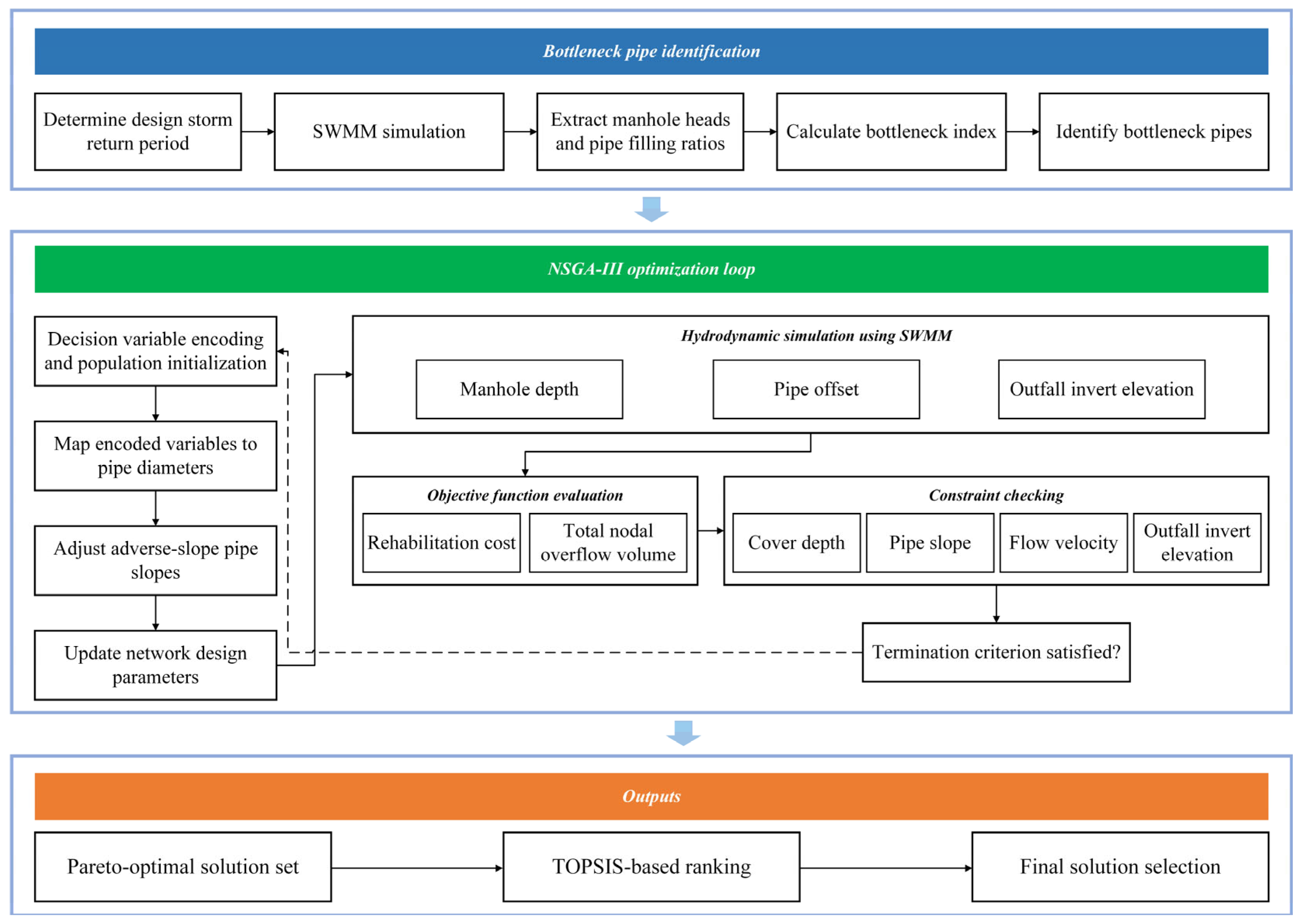
The overall optimization framework is illustrated in Figure 1. As shown in the figure, the process begins with input data preparation, followed by the construction and calibration of the hydrodynamic model of the existing drainage network. Then, bottleneck pipes are identified and the multi-objective optimization model is established. Based on the decision variables generated by the NSGA-III algorithm, the corresponding pipe diameters are updated according to the predefined commercial diameter set, and the modified drainage network is simulated in SWMM under the design rainfall conditions. The simulation results are used to calculate the objective function values, which are then returned to the optimization algorithm for population updating through non-dominated sorting, reference-point-based selection, crossover, and mutation. This iterative simulation–optimization process continues until the termination criterion is satisfied, yielding a set of Pareto-optimal solutions for the subsequent selection of the optimal rehabilitation scheme.

2.1. Study Area

Fuzhou, located on the southeastern coast of China, is the capital city of Fujian Province. Its urban area mainly consists of two parts: the northern urban district and Nantai Island. In this study, the Sanjie River catchment, located in the northern urban district, was selected as the study area. This area is a typical coastal intermontane basin.

The northern urban district is situated in the center of Fuzhou, with terrain generally characterized by higher elevations in the west and north and lower elevations in the south. It is surrounded by mountains on the east, west, and north sides, while the southern side is adjacent to the Minjiang River. Fuzhou has a maritime subtropical monsoon climate, with an annual average precipitation ranging from 900 to 2100 mm and is affected by approximately four typhoons each year on average.

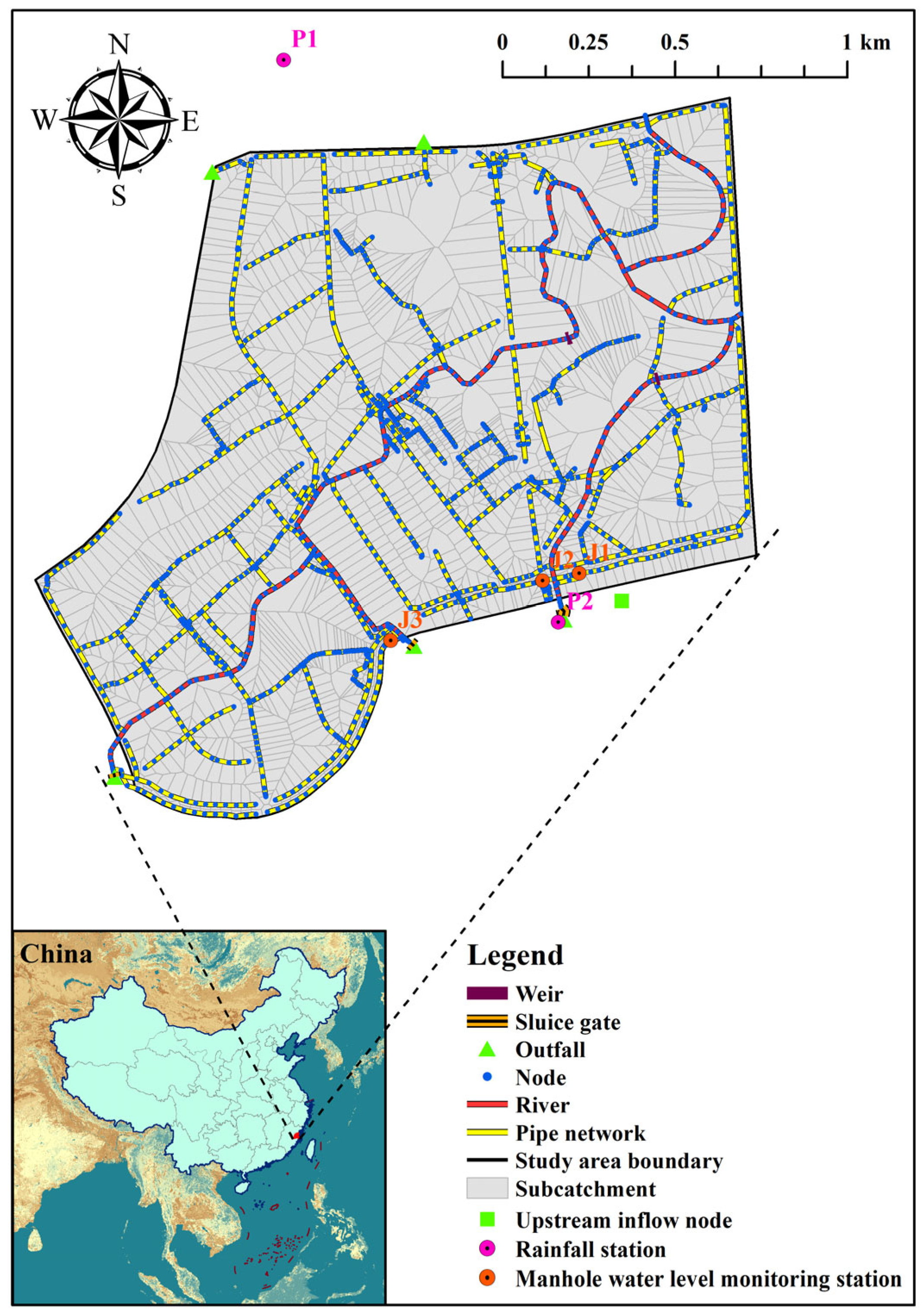
The distribution of the drainage network model in the study area is shown in Figure 2. The study area covers 273.8 ha. During model development, the original drainage network was reasonably generalized by removing some branch pipes and merging drainage pipes located on both sides of main roads with the same flow direction through cross-sectional area superposition. The final drainage network model consisted of 1501 pipes, including 278 river channels, 1464 nodes, 3668 subcatchments, 5 outfalls, and 3 sluice gates. The DEM used in this study had a spatial resolution of 2 m, and the river network model was constructed using channel cross-sectional data with a spacing of 2 m.

2.2. Hydrodynamic Modeling of the Drainage Network

2.2.1. SWMM

The Storm Water Management Model (SWMM) is a dynamic rainfall–runoff model developed by the United States Environmental Protection Agency (EPA). It was first released in 1971 and has since undergone several version upgrades. At present, it has been widely applied in urban stormwater flooding research as well as in the planning, analysis, and design of drainage systems [19]. In this study, the dynamic wave method was adopted as the routing method because it can account for channel storage, backwater effects, flow reversal, and pressurized flow [20]. SWMM solves the water levels and flow rates in nodes and conduits simultaneously by coupling the Saint-Venant equations, which are expressed as follows [21]:

(1) 

Continuity Equation

$${\displaystyle \frac{\partial A}{\partial t}}+{\displaystyle \frac{\partial Q}{\partial x}}=0$$

(1)

(2) 

Momentum Equation

$${\displaystyle \frac{\partial Q}{\partial t}}+{\displaystyle \frac{\partial \left(Q^2/A\right)}{\partial x}}+gA{\displaystyle \frac{\partial H}{\partial x}}+gA{S}_f=0$$

(2)

where x is the distance [m]; t is the time [s]; A is flow cross-sectional area [m²]; Q is flow rate [m³/s]; H is hydraulic head of water in the conduit [m]; S_f is the friction slope (head loss per unit length); g is acceleration of gravity [m/s²].

In the present study, the EPA’s SWMM version 5.2 software was used for hydrological and hydraulic simulation of the pipeline network. The Sanjie River catchment includes two sluice gates along the inner river network and three sluice gates along the outer river. In this study, control rules for these sluice gates were incorporated into the model, and tidal boundary conditions were assigned to the outfalls connected to the sluice gates.

2.2.2. Evaluation Metrics

The performance of the SWMM during parameter calibration was evaluated using several statistical metrics, including the correlation coefficient (CC), percent bias (PBIAS), mean absolute error (MAE), root mean square error (RMSE), and Nash–Sutcliffe efficiency coefficient (NSE) [22].

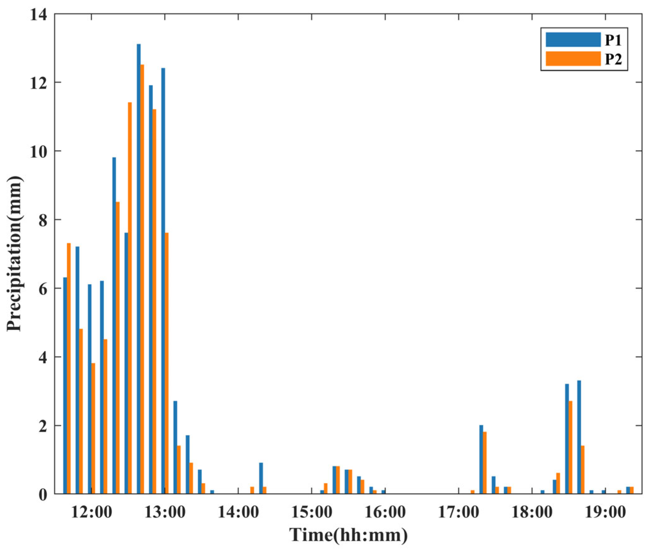
Two rainfall gauges (

Table 1. Information of rainfall gauges.

No.	Station No.	Station ID	X	Y
1	350103020004	P1	430,103.61	2,884,741.1
2	350103020005	P2	430,901.09	2,883,105.8

) and three manhole water level monitoring stations (

Table 2. Information on water level monitoring stations in rainwater wells.

No.	Station No.	Station ID	X	Y
1	350103130242	J1	430,961.08	2,883,247.92
2	350103130238	J2	430,854.89	2,883,226.32
3	350102130248	J3	430,414.65	2,883,052.49

) were established in the study area. Because the monitoring data quality in the study area was relatively poor, only limited observations were suitable for model calibration. Therefore, the data from the rainfall event occurring between 11:40 and 19:20 on 5 August 2021, were selected to calibrate the drainage network model parameters.

As shown in Figure 3, this rainfall event exhibited relatively high intensity during the initial stage and then gradually weakened, showing an overall multi-peak distribution pattern. The rainfall duration was 460 min, with a temporal resolution of 10 min. The cumulative rainfall amounts recorded at rainfall gauges P1 and P2 were 99.2 mm and 84.2 mm, respectively, while the corresponding maximum rainfall intensities were 1.31 mm/min and 1.25 mm/min, respectively.

2.3. Design Rainfall Estimation

2.3.1. Rainfall Intensity Formula

The urban design rainfall intensity formula adopted for the main urban area of Fuzhou was derived from the Rainfall Intensity Formulas for Cities and Selected County Towns in Fujian Province (Draft for Comments). This formula was developed based on minute-level rainfall observations collected at the Jin’an Meteorological Station during 1982–2012, using the annual maximum method, and the rainfall intensity formulas expressed as follows:

$$q={\displaystyle \frac{A_1\left(1+CLgP\right)}{{\left(t+b\right)}^n}}$$

(3)

where q is the rainfall intensity [L/(s·hm²)]; t is the rainfall duration [min]; P is the design return period [years], and A₁, C, b, and n are parameters determined using statistical methods.

If q needs to be converted to mm/min, the right-hand side of the above equation should be divided by 167. The adopted parameter values for Fuzhou were (A₁ = 2457.435), (C = 0.633), (b = 11.951), and (n = 0.724).

2.3.2. Design Storm Pattern

The rainfall hyetograph input to the SWMM was designed using the Chicago rainfall pattern [23], with the peak coefficient set to 0.4. The calculation formula is as follows:

$$R_T=q_t\times t$$

(4)

$$\left\{\begin{array}{ll}{i}_b=R_T\times \left(r-\left(r-{\displaystyle \frac{t}{T}}\right){\left(1-{\displaystyle \frac{t}{r\left(T+b\right)}}\right)}^{-n}\right)& ,0\le t\le rT\\ i_a=R_T\times \left(r+\left({\displaystyle \frac{t}{T}}-r\right){\left(1+{\displaystyle \frac{t-T}{\left(1-r\right)\left(T+b\right)}}\right)}^{-n}\right)& ,rT<t\le T\end{array}\right.$$

(5)

where i_a and i_b are the rainfall intensities before and after the rainfall peak, respectively [mm/min]; r is the ratio of pre-peak duration to total duration; T is the storm duration [min]; b and n are constants of storm intensity formula; t is the time in minutes from start of storm [min]; R is the total precipitation [mm].

The 3-, 5-, 10-, and 20-year return periods were selected for rehabilitation optimization because they are commonly used in the planning and design of urban stormwater drainage systems and represent progressively increasing levels of design rainfall severity.

2.4. Bottleneck Pipe Identification Method

This study proposes an improved method for calculating the bottleneck index. The method first uses the hydraulic heads at the upstream and downstream nodes of a full-flow pipe to calculate the actual hydraulic gradient of the pipe, and then determines the absolute value of the ratio between the actual hydraulic gradient and the pipe slope. Subsequently, the final bottleneck index is obtained by incorporating the pipe filling degree. This index is mainly used to identify pipe sections with insufficient drainage capacity and unreasonable construction conditions. The calculation formula is as follows:

$${\phi }_{\mathrm{i}}=\left\{\begin{array}{l}{\gamma }_{\mathrm{i}}, {\beta }_i=1\\ 0, {\gamma }_{\mathrm{i}}>1 and {\beta }_i<1\\ {\gamma }_{\mathrm{i}}, {\gamma }_{\mathrm{i}}<1 and {\beta }_i<1\end{array}\right.$$

(6)

$${\gamma }_{\mathrm{i}}=\left|{\displaystyle \frac{\left(H_{up}-H_{dowm}\right)/l_i}{i_i}}\right|$$

(7)

$${\beta }_{\mathrm{i}}={\displaystyle \frac{h}{D}}$$

(8)

where ${\phi }_{\mathrm{i}}$ is the bottleneck index of the ith pipe; ${\gamma }_{\mathrm{i}}$ is the absolute value of the ratio between the actual hydraulic gradient and the pipe slope of the ith pipe; ${\beta }_i$ is pipe filling ratio of the ith pipe; $H_{up}$ is the hydraulic head of the stormwater manhole connected to the upstream end of the ith pipe [m]; $H_{dowm}$ is the hydraulic head of the stormwater manhole connected to the downstream end of the ith pipe [m]; $l_i$ is the horizontal length of the ith pipe [m]; $i_i$ is the slope of the ith pipe; h is the water depth in the ith pipe [m]; and D is the diameter of the ith pipe [m].

For the horizontal length of a pipe, because the design slope is usually small, engineering practice commonly approximates the actual pipe length as its horizontal projected length. However, owing to unreasonable factors arising during pipe network construction and operation, such as local construction deviations and structural deformation, pipe displacement may occur at certain locations, thereby increasing the actual pipe slope. Therefore, in this study, the horizontal length of each pipe was calculated using the coordinates of its upstream and downstream nodes. For pipes whose upstream and downstream crown elevations are equal, to avoid a zero slope that would cause the bottleneck index to approach infinity, the pipe slope was uniformly assigned as the minimum slope specified by the design standard, i.e., 0.003.

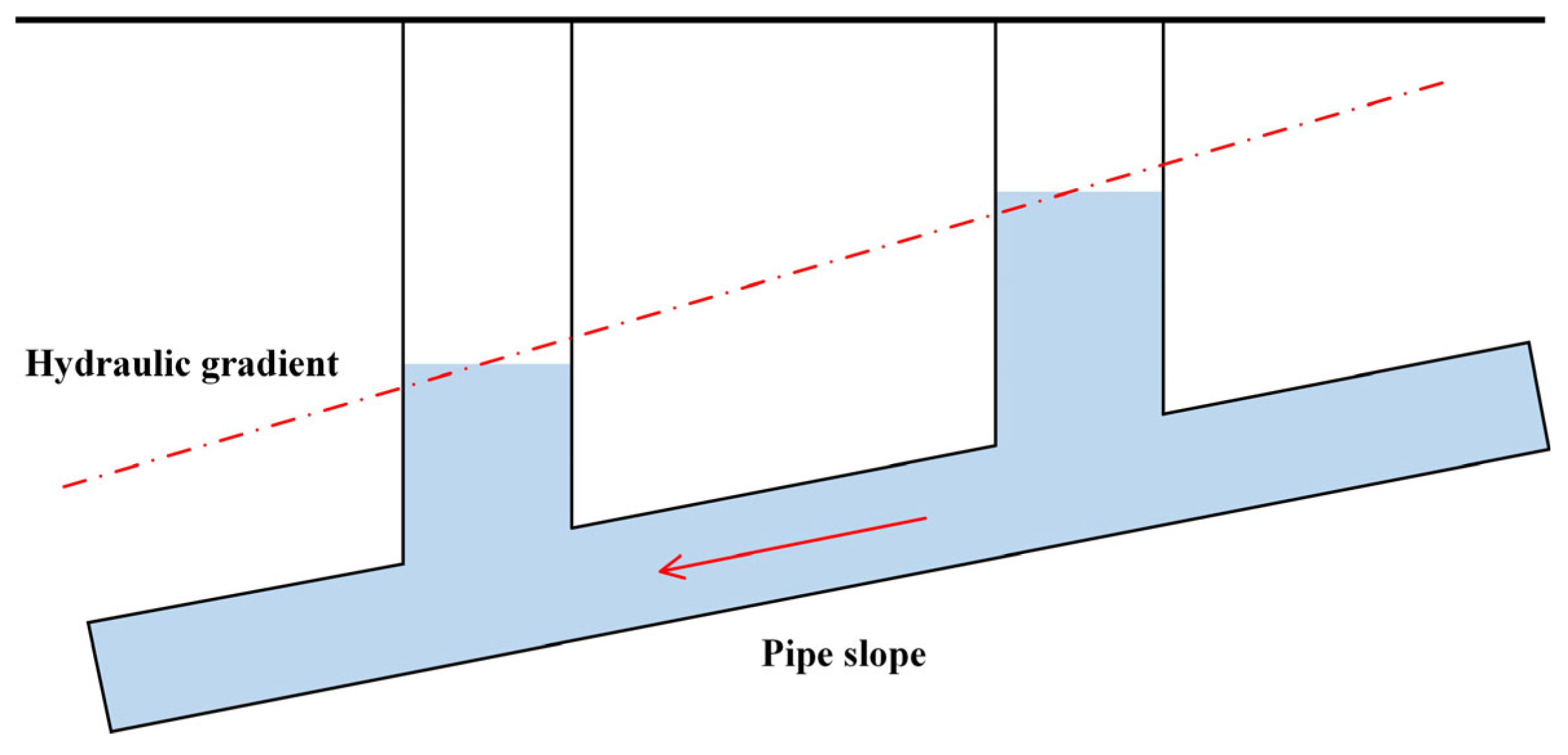
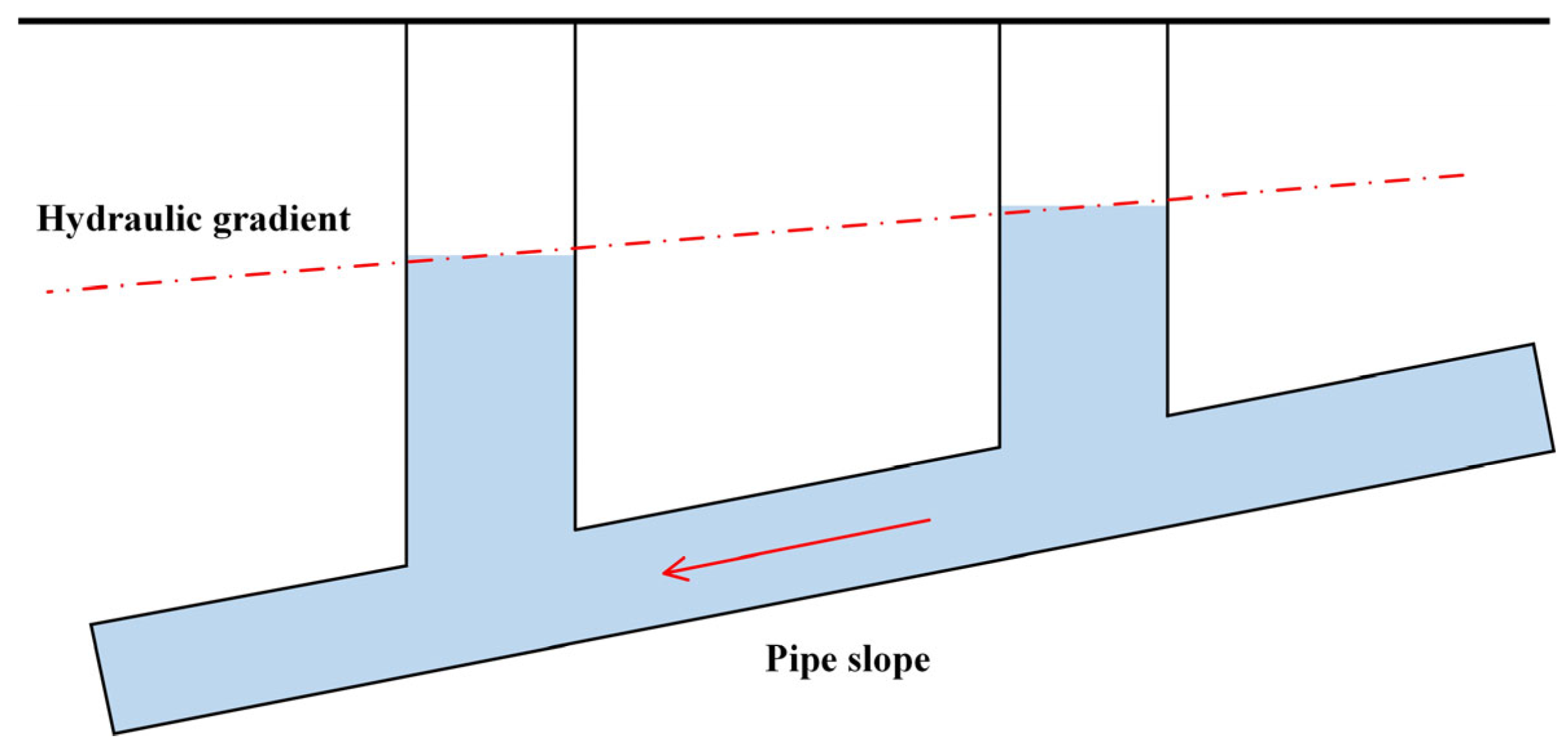
The slope relationship of bottleneck pipes is illustrated in Figure 4 and Figure 5. When ${\phi }_{\mathrm{i}}$ > 1, the actual pipe flow exceeds the design flow, indicating that the design standard of the pipe is insufficient; therefore, the pipe can be identified as a bottleneck pipe. When ${\phi }_{\mathrm{i}}$ < 1, the actual pipe flow is lower than the design flow, indicating that the pipe still has surplus drainage capacity and retains a certain degree of internal storage potential. The threshold (BI = 1) was adopted as the critical value for bottleneck pipe identification. This threshold (${\phi }_{\mathrm{i}}$ = 1) was derived from the physical meaning of the proposed bottleneck index and further verified using the hydrodynamic simulation results under different design rainfall conditions. Specifically, the pipe filling ratio and the hydraulic heads of the upstream and downstream stormwater manholes were extracted from the SWMM simulation results and used to calculate the bottleneck index for a large number of pipe. The verification results indicated that (${\phi }_{\mathrm{i}}$ = 1) provides a physically meaningful boundary between bottleneck and non-bottleneck pipes. For an individual pipe, the upstream and downstream nodal heads simulated by SWMM are time series. Accordingly, bottleneck pipes can be identified either based on the results at a specific time step or by analyzing the maximum bottleneck index over all time steps, that is, by adopting the bottleneck index corresponding to the most unfavorable moment as the final criterion for identification.

2.5. Multi-Objective Optimization Model

2.5.1. Decision Variables

Based on the evaluation results of the improved bottleneck index (BI), the candidate pipes for rehabilitation include both bottleneck pipes (BI > 1) and pipes directly connected to the river, so as to prevent downstream overflow caused by insufficient downstream conveyance capacity after upstream capacity expansion. Other non-bottleneck pipes retain their original dimensions. The set of pipes to be optimized, denoted as ${\mathrm{\Omega }}_{opt}$, is defined as:

$${\mathrm{\Omega }}_{opt}=\left\{i\in \mathrm{\Omega }|B{I}_i>1\right\}\cup \left\{i\in {\mathrm{\Omega }}_{river}\right\}$$

(9)

where $\mathrm{\Omega }$ is the set of all pipelines in the network, BI_i is the bottleneck index of pipe i, and ${\mathrm{\Omega }}_{river}$ is the set of pipes discharging into the river.

The decision variables for the optimization model are the enlargement levels of the pipe diameters, denoted as x_i. To avoid over-design and ensure that the diameters of the replaced pipes do not exceed the maximum allowable diameter for post-retrofitting pipes within the range of commercially available sizes, an upper bound on pipe diameter is imposed. Let C denote the ordered set of commercially available pipe diameters, and let k_max denote the index of the maximum allowable diameter for post-retrofitting pipes. If the original diameter $D_i^{old}$ corresponds to the k-th index in set C, the upgraded diameter $D_i^{new}$ is determined by:

$$D_i^{new}=\left\{\begin{array}{l}{C}_{\min \left(k+x_i,k_{\max }\right)}, if i \in {\mathrm{\Omega }}_{opt}\\ D_i^{old} , if i \notin {\mathrm{\Omega }}_{opt}\end{array}\right.$$

(10)

This constraint guarantees that any decision variable yielding a diameter larger than the predefined maximum limit is capped at the maximum allowable commercial diameter.

2.5.2. Objective Functions

(1) Rehabilitation cost

The total cost of pipe network rehabilitation consists of both the construction cost and the demolition cost of stormwater facilities, and is calculated as follows:

$$f_1=\min \left(\left(1+k\right)\left({\displaystyle {\displaystyle \sum _{i=1}^m}{C}_{i,pipe}{L}_{i,pipe}}+{\displaystyle {\displaystyle \sum _{j=1}^n}{C}_{j,junc}}\right)+{\displaystyle \sum _{k=1}^p{C}_{k,pump}}\right)$$

(11)

where f denotes the total cost of pipe network rehabilitation [CNY]; k is the proportional coefficient for the demolition cost of stormwater facilities, which was set to 0.2 in this study; C_i,pipe denotes the unit cost per unit length of the i-th pipe [CNY]; L_i,pipe denotes the length of the i-th pipe [m]; and C_k,pump denotes the construction cost of the k-th stormwater pumping station [CNY].

(2) Total nodal overflow volume

The total overflow volume of stormwater manholes was used as the evaluation indicator to characterize the drainage performance after pipe network rehabilitation. A smaller value of this indicator indicates better drainage performance of the pipe network, and it was calculated as follows:

$$f_2=\min \left(V_{overflow}\right)$$

(12)

$$V_{overflow}=60\times {\displaystyle \sum _{i=1}^n{\displaystyle \sum _{j=1}^t{Q}_{i,t,overflow}}}$$

(13)

where $V_{overflow}$ is the total overflow volume at all nodes [m³]; n is the total number of nodes; t is the simulation duration [min]; and $Q_{i,t,overflow}$ is the overflow discharge at node i at time t [m³/s].

2.5.3. Constraints

The model constraints include pipe slope, flow velocity, burial depth, and outlet invert elevation, as follows:

(1) pipe slope

$$I_{\min }\le I_i\le I_{\max }$$

(14)

where I_i is the design slope of pipe i; I_min is the minimum allowable design slope, set to 0.003; I_max is the maximum allowable design slope, set to 0.05.

(2) flow velocity

The allowable range of design flow velocity for drainage pipe networks is specified as follows. For the maximum design flow velocity, the limits are 10 m/s for metal pipes and 5 m/s for non-metal pipes. For the minimum design flow velocity, the limits are 0.6 m/s for sanitary sewers, 0.75 m/s for stormwater pipes, and 0.4 m/s for open channels. For stormwater open channels, the corresponding design flow velocity and conversion coefficient should be selected according to the flow depth and channel type. Since all drainage facilities considered for rehabilitation in this study are circular pipes and do not involve open channels, calculations related to open channels were not considered.

$$v_{\min }\le v_i\le v_{\max }$$

(15)

where v_i is the design flow velocity of pipe i [m/s]; v_min is the minimum allowable design flow velocity [m/s]; v_max is the maximum allowable design flow velocity [m/s].

(3) burial depth

The minimum cover depth above the pipe crown is specified as 0.6 m beneath sidewalks and 0.7 m beneath roadways. Since the study area is located in Fuzhou, where the average winter temperature is above 0 °C, frost heave does not occur in the soil; therefore, the effects of the frost line and thermal insulation measures on pipe burial depth were not considered. The burial depth of a pipe is defined as the sum of the cover depth and the pipe diameter. To reduce construction costs, the maximum burial depth was set to 5 m in this study.

$$H_{\min }\le H_{i,up}\le H_{\max }$$

(16)

$$H_{\min }\le H_{i,down}\le H_{\max }$$

(17)

where H_i,up denotes the burial depth at the upstream end of pipe i [m]; H_i,down denotes the burial depth at the downstream end of pipe i [m]; H_min denotes the minimum allowable burial depth [m]; and H_max denotes the maximum allowable burial depth [m].

(4) outlet invert elevation

The downstream end of each pipe to be optimized is connected to an outlet, and the outlet invert elevation is taken as the pipe invert elevation at the downstream end. This elevation should fall within the elevation range of the river cross-section and satisfy the burial depth constraints. In general, the outlet invert elevation should be higher than the normal river water level or the multi-year average flood level. In this study, the constraints only restrict its allowable range, i.e., requiring it to lie within the river cross-sectional elevation range. Meanwhile, the objective function calculates the average cover depth from the top of the river outlet to the ground surface and minimizes this value through optimization. This treatment enables the flow within the pipe to be discharged, as far as possible, under conditions higher than the normal river water level, thereby improving the operational capacity of the drainage system during flood events and reducing the possibility of river floodwater backflowing into the drainage system and causing urban waterlogging during heavy rainfall.

$$Z{R}_{\min }\le Z_{out}\le Z{R}_{\max }-D_{end}$$

(18)

where Z_out denotes the outlet invert elevation [m]; ZR_min denotes the bottom elevation of the river cross-section where the downstream pipe end is located [m]; ZR_max denotes the top elevation of the river cross-section where the downstream pipe end is located [m]; and D_end denotes the diameter of the downstream terminal pipe [m].

2.5.4. Optimization Algorithm (NSGA-III)

This study employed the NSGA-III algorithm proposed by Deb et al. [24] in 2014, which is capable of solving multi-objective optimization problems involving 2 to 15 objective functions. The core idea of the NSGA series algorithms is to perform individual selection through non-dominated sorting and population diversity control. Unlike NSGA-II, which relies on a crowding-distance-based selection strategy, NSGA-III guides population distribution by introducing uniformly distributed reference points on a normalized hyperplane, thereby maintaining the diversity of the solution set more effectively.

For the NSGA-III optimization, the population size was set to 200. The crossover probability was set to 1.0, and the mutation probability for each decision variable was set to 1/D, where D is the number of decision variables. The termination criterion was defined as a maximum of 10,000 function evaluations, calculated as the product of the population size and the number of generations, corresponding to 50 generations. Parallel computing with 48 CPU cores was adopted to improve computational efficiency. Under these settings, the optimization time was approximately 2.4 h for each return-period scenario.

2.5.5. Optimization Method

Step 1:

Preprocess the calibrated model. For tree-structured drainage networks, the pipe flow directions are uniformly corrected according to the outlet locations so that all pipes discharge toward the outlets. For looped drainage networks, the pipe flow directions are corrected based on the contributing catchment areas, following the principle of uniformly distributing the converging flow.

Step 2:

Based on the specified design return period, SWMM is used to simulate the corrected pipe network model. Bottleneck pipes under the design return period are identified, and their IDs are extracted. Meanwhile, the IDs of non-bottleneck pipes connected to the river are also extracted. The IDs of these two categories of pipes are then combined to determine the pipes to be rehabilitated.

Step 3:

The pipe slope is calculated according to the pipe flow direction, and adverse-slope pipes are identified and corrected. During the correction process, when the invert elevation of the downstream manhole is higher than that of the upstream manhole, and both the upstream and downstream pipe invert elevations are assigned as the corresponding manhole invert elevations, the pipe may still exhibit an adverse slope. To address this issue, the upstream pipe offset is increased, and the downstream end of the pipe is connected to the downstream manhole invert according to the design slope, thereby correcting the adverse slope. Considering that excavation and backfilling should be minimized during rehabilitation and that the original burial depth conditions of the existing pipe network and manholes should be utilized as much as possible, the crown-to-crown alignment constraint between upstream and downstream pipes was neglected in the rehabilitation design.

Step 4:

The corresponding commercial discrete pipe diameter is determined according to the value of the decision variable. If the resulting diameter exceeds the maximum allowable diameter for post-retrofitting pipes, the maximum allowable diameter is adopted. The slope of the rehabilitated pipe is then determined based on the slope calculation method used in the optimization design. When the flow velocity is lower than the minimum design flow velocity specified by the design standard, the design slope is increased accordingly. The design slope of the rehabilitated pipe is calculated as follows:

(1)

Based on the rehabilitated pipe diameter D and the minimum and maximum allowable design flow velocities specified in the constraint conditions, the allowable range of the pipe slope $I^{\prime }$ can be back-calculated.

$$I^{\prime }\in \left[I_{\min }^{\prime },I_{\max }^{\prime }\right]$$

(19)

$$I_{\min }^{\prime }={\left({\displaystyle \frac{v_{\min }n}{\sqrt[3]{R^2}}}\right)}^2$$

(20)

$$I_{\max }^{\prime }={\left({\displaystyle \frac{v_{\max }n}{\sqrt[3]{R^2}}}\right)}^2$$

(21)

For stormwater pipes:

$$R={\displaystyle \frac{D}{4}}$$

(22)

For sewer pipes:

$$R={\displaystyle \frac{D}{4}}\left({\displaystyle \frac{\theta -\sin \theta }{\theta }}\right)$$

(23)

$$\theta =2\arccos \left(1-2{\left({\displaystyle \frac{h}{D}}\right)}_{\max }\right)$$

(24)

where $I_{\min }^{\prime }$ denotes the minimum design slope of the pipe; $I_{\max }^{\prime }$ denotes the maximum design slope of the pipe; v_min denotes the minimum allowable design flow velocity [m/s]; v_max denotes the maximum allowable design flow velocity [m/s]; n denotes the Manning roughness coefficient of the pipe, which was set to 0.013 in this study; D denotes the pipe diameter [m]; R denotes the hydraulic radius [m]; $\theta$ denotes the central angle corresponding to the water surface relative to the center of the pipe cross-section [rad]; ${\left({\displaystyle \frac{h}{D}}\right)}_{\max }$ denotes the maximum allowable design flow depth ratio of the pipe.

According to the Chinese design standard for outdoor drainage, the minimum design flow velocity for stormwater pipes and combined sewers under full-flow conditions should not be less than 0.75 m/s. The maximum design flow velocity for non-metallic drainage pipes is generally specified as 5 m/s and may be appropriately increased when justified by experimental verification. Therefore, in this study, the minimum allowable design flow velocity v_min was set to 0.75 m/s, and the maximum allowable design flow velocity v_max was set to 5 m/s.

(2)

Based on the calculated values of $I_{\min }^{\prime }$ and $I_{\max }^{\prime }$, together with the relative relationship among the design-standard-specified I_min and I_max and the ground slope I_g, the design slope of the pipe is determined as follows:

$$I_{pipe}=\left\{\begin{array}{cc}{I}_{\min }& I_{\max }^{\prime }\le I_{\min }\\ I_{\min }& I_{\min }^{\prime }\le I_{\min },I_{\max }^{\prime }\ge I_{\min } and I_{\mathrm{g}}\notin \left[I_{\min },\min \left(I_{\max }^{\prime },I_{\max }\right)\right]\\ I_g& I_{\min }^{\prime }\le I_{\min },I_{\max }^{\prime }\ge I_{\min } and I_{\mathrm{g}}\in \left[I_{\min },\min \left(I_{\max }^{\prime },I_{\max }\right)\right]\\ I_{\min }^{\prime }& I_{\min }\le I_{\min }^{\prime }\le I_{\max } and I_{\mathrm{g}}\notin \left[I_{\min }^{\prime },\min \left(I_{\max }^{\prime },I_{\max }\right)\right]\\ I_g& I_{\min }\le I_{\min }^{\prime }\le I_{\max } and I_{\mathrm{g}}\in \left[I_{\min }^{\prime },\min \left(I_{\max }^{\prime },I_{\max }\right)\right]\\ I_{\max }& I_{\max }^{\prime }\ge I_{\min }\end{array}\right.$$

(25)

When the ground slope falls within the overlapping allowable range of $[I_{\min }^{\prime },I_{\max }^{\prime }]$ and $[I_{\min },I_{\max }]$, it is preferentially adopted as the pipe slope. When the pipe slope is consistent with the ground slope, both construction difficulty and subsequent operation and maintenance costs can be reduced. In addition, when the upstream ground slope is relatively steep while the downstream ground slope is relatively gentle, adopting the ground slope as the pipe slope can prevent the cover depth of the downstream pipe from being less than 0.7 m.

After the design slope is calculated, if the design flow velocity of the pipe is still lower than the minimum value required by the design standard, the design slope is further increased.

Step 5:

The SWMM INP file is updated and hydrodynamic simulations are performed. The time series of nodal overflow discharge are then extracted to calculate the rehabilitation cost of the pipe network and the total nodal overflow volume.

Step 6:

Examine whether the design parameters of all pipes in the updated optimization scheme satisfy the constraint conditions.

Step 7:

After the iteration is completed, Pareto-optimal solutions are screened from the feasible solutions satisfying all constraint conditions. The Pareto-optimal solutions are then further evaluated using the TOPSIS [25] method, and the final optimal rehabilitation scheme that meets the engineering design requirements is determined.

3. Results

3.1. Parameter Calibration of the Drainage Network Model

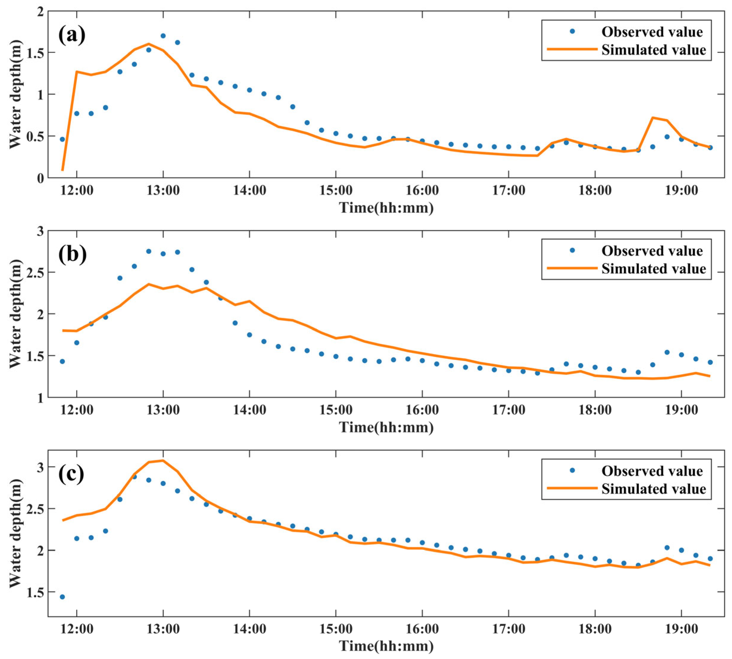
The simulation results of water depth in stormwater manholes are shown in Figure 6. Overall, the simulated values at each monitoring site are generally consistent with the observed values in terms of temporal variation, indicating that the established drainage network model can effectively capture the dynamic process of manhole water depth. At station J3, the observed initial water depth was relatively small, being less than 1.5 m, whereas the corresponding simulated value was comparatively higher. Given that rainfall was mainly concentrated in the early stage of the simulation and that no rainfall occurred during 14:00–15:00, the drainage network should have had relatively favorable drainage conditions during this period. However, the water depth remained at approximately 2 m, which was significantly higher than the initial observed value. Therefore, it is inferred that the observed initial water depth data at this station may contain anomalies. At station J2, the simulation error for the peak water depth was relatively large, with the peak occurring at 12:50 and an error of 0.39 m. In contrast, the simulated peak water depth at station J1 was in closer agreement with the observed value, with a peak error of 0.18 m.

As shown in

Table 3. Accuracy evaluation of simulated water depths in stormwater manholes.

Station ID	PBIAS	CC	MAE	NSE	RMSE
J1	0.85%	0.88	0.10	0.66	0.18
J2	0.86%	0.86	0.18	0.74	0.22
J3	−5.46%	0.88	0.14	0.74	0.20

, the CC values at all monitoring sites are close to 0.9, and the NSE values remain around 0.7. Specifically, the PBIAS values at stations J3 and J2 are both less than 1%, while that at station J1 is less than 6%. In addition, the MAE and RMSE values at all sites are relatively low. Overall, the established drainage network model exhibits good simulation accuracy and applicability, and can realistically reproduce the variation process of stormwater manhole water levels in the study area. It should be noted that the model calibration was conducted using a single rainfall event because of limited high-quality monitoring data in the study area. Further validation using additional rainfall events would help improve the robustness of the proposed framework.

3.2. Temporal Evolution and Spatial Distribution of Bottleneck Pipes

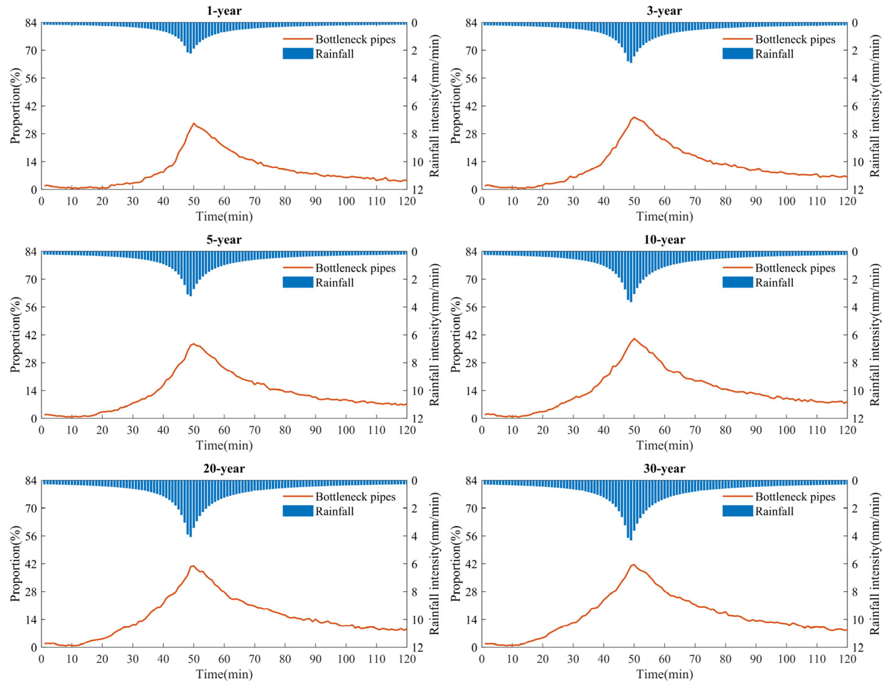
Figure 7 presents the proportion of bottleneck pipes at each simulation time step, as calculated using the improved bottleneck index method under different return-period conditions. It can be observed that the temporal variation in the proportion of bottleneck pipes is generally consistent with the rainfall process. At the early stage of rainfall, the proportion of bottleneck pipes is very low, being less than 2% and close to zero. For design storms with return periods of 1, 3, 5, 10, 20, and 30-year, the maximum proportions of bottleneck pipes are 33.28%, 36.30%, 37.53%, 40.07%, 40.96%, and 41.62%, respectively. As the storm return period increases, the maximum proportion of bottleneck pipes gradually rises. However, under larger return-period conditions, the rate of increase becomes significantly smaller and exhibits a saturation trend, with the results for the 10-, 20-, and 30-year design storms being relatively similar.

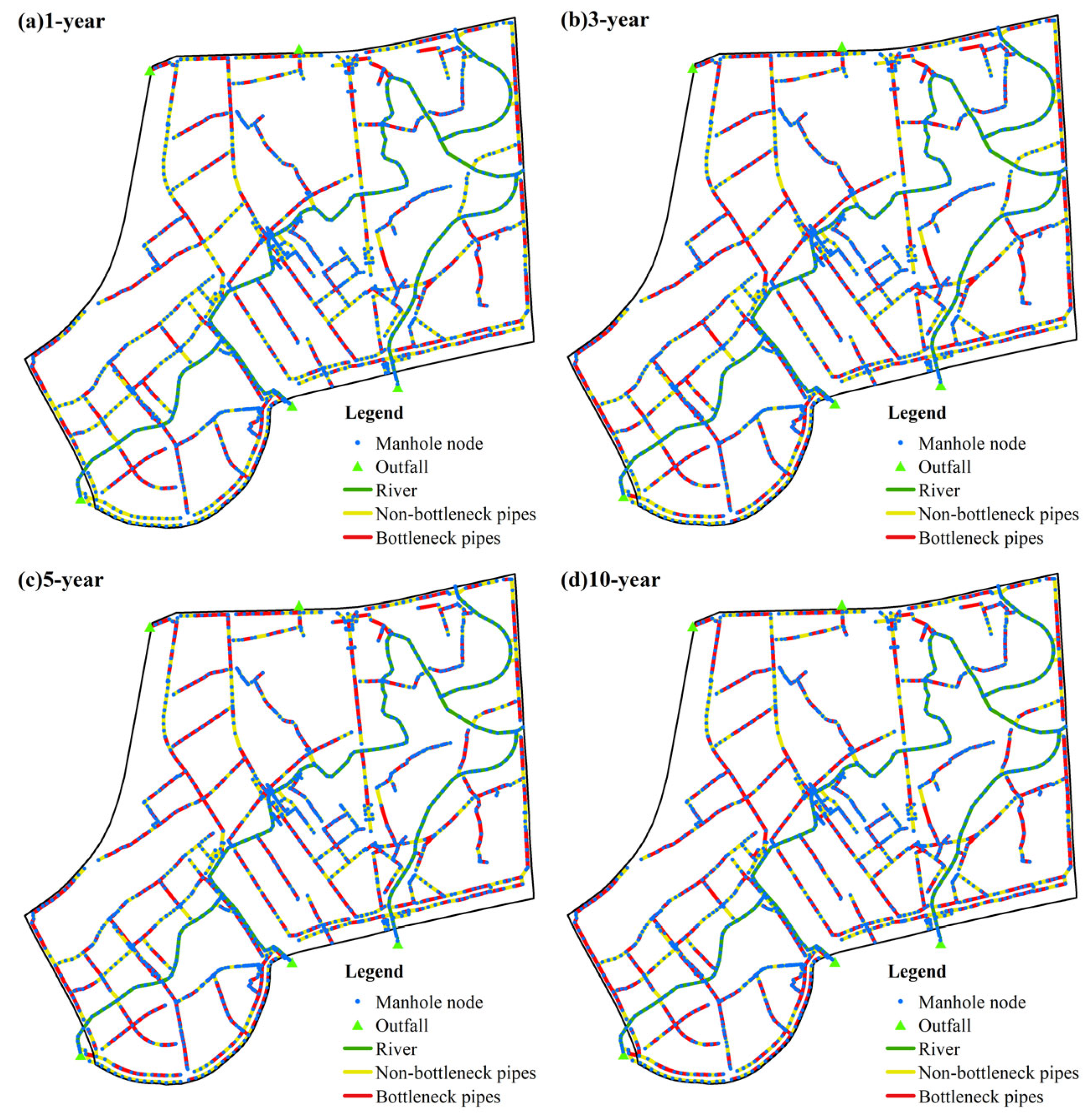
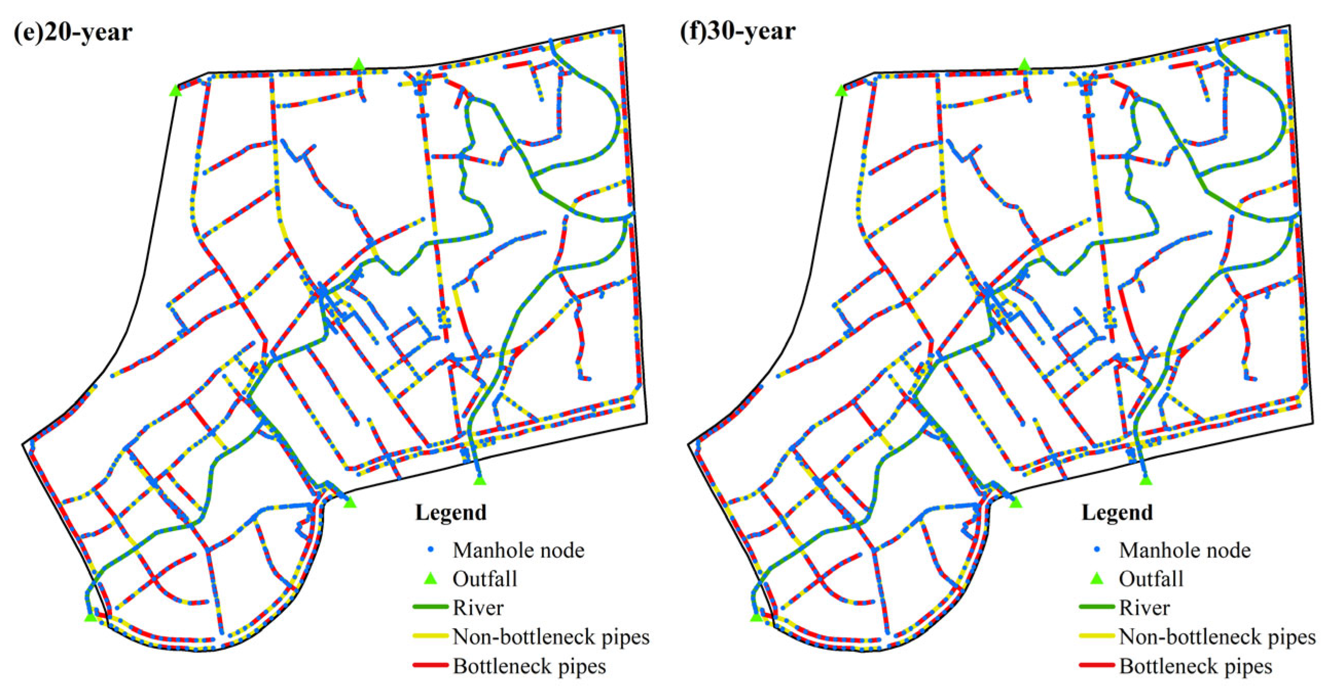
The spatial distribution of bottleneck pipes under different return-period conditions is shown in Figure 8. It can be seen that a certain number of bottleneck pipes are present in all areas of the Sanjie River Basin, and the bottleneck pipes identified under small return-period design storms are generally included within those identified under larger return-period conditions. Overall, the spatial distribution of bottleneck pipes is relatively scattered, indicating that their adverse impacts on the drainage system are widespread and may increase the likelihood of large-scale urban waterlogging. Therefore, future rehabilitation and expansion efforts should focus on these bottleneck pipes to enhance the overall drainage capacity of the pipe network. In addition, the identification results of these bottleneck pipes can also provide a basis for selecting decision variables in the multi-objective optimization design model for pipe network rehabilitation.

3.3. Multi-Objective Optimization Results and Decision Analysis

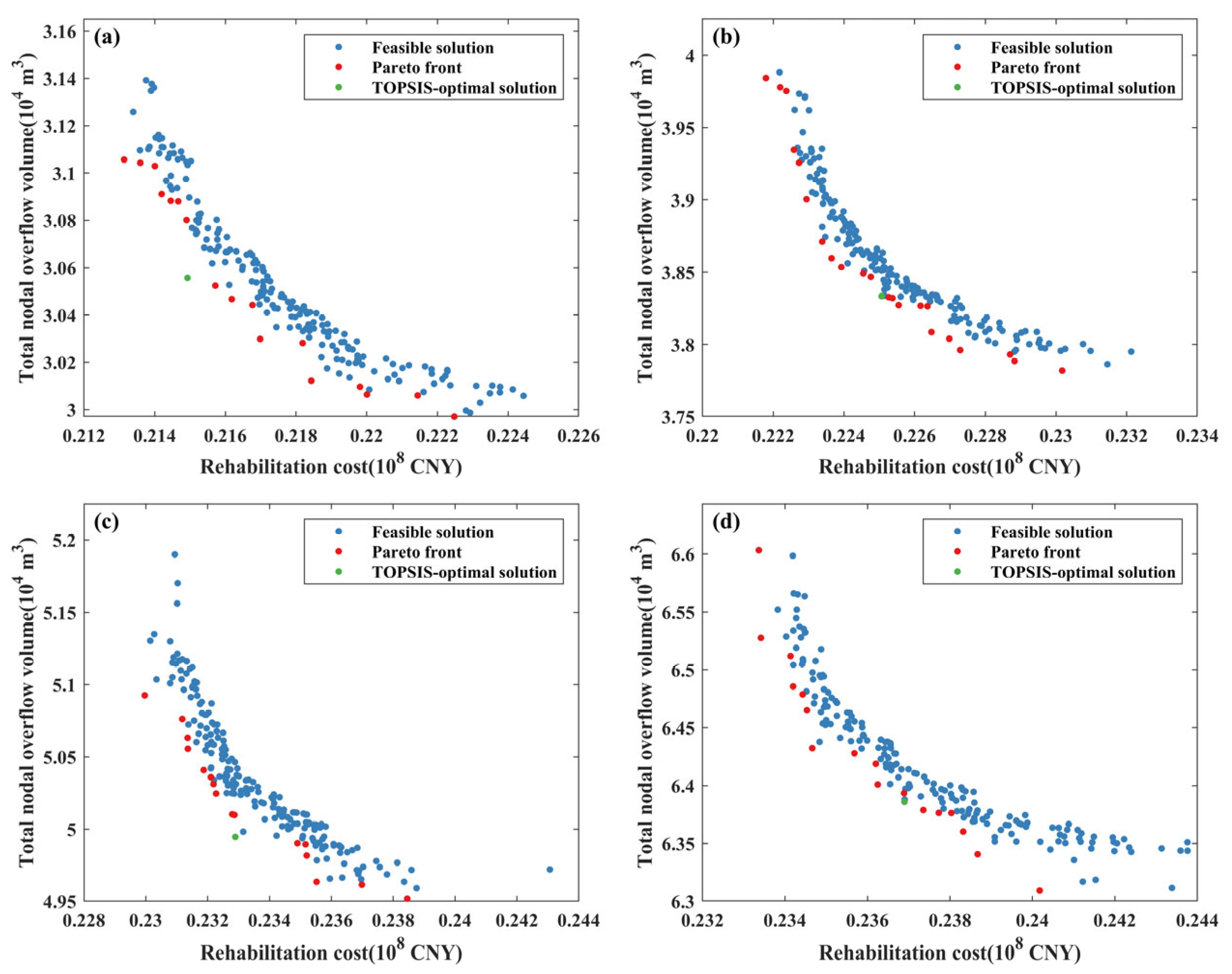
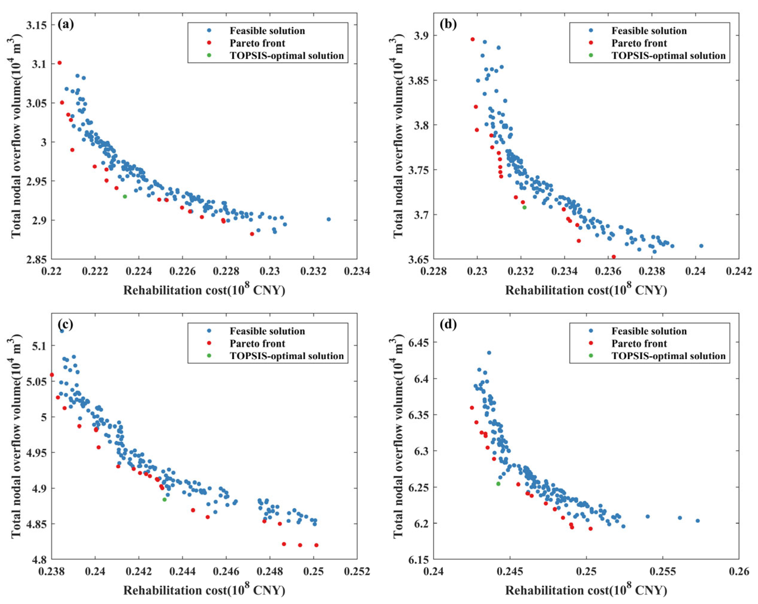
In this study, the maximum allowable pipe diameters after rehabilitation were set to 1.2 m and 1.5 m, respectively. The maximum expansion level of the pipe diameter was set to 4. Under different return-period conditions, the multi-objective optimization results are shown in Figure 9 and Figure 10. The results indicate that the total nodal overflow volume generally decreases as the rehabilitation cost increases. The TOPSIS ranking results are presented in

Table 4. TOPSIS-optimal solutions for different return periods and maximum allowable diameters for post-retrofitting pipes.

Maximum Allowable Pipe Diameter After Rehabilitation	Rehabilitation Cost (108 CNY)				Total Nodal Overflow Volume (104 m3)
	3-Year	5-Year	10-Year	20-Year	3-Year	5-Year	10-Year	20-Year
1.2 m	0.215	0.225	0.233	0.237	3.056	3.833	4.995	6.386
1.5 m	0.223	0.232	0.243	0.244	2.930	3.708	4.884	6.255
Percentage change of 1.5 m relative to 1.2 m	3.92%	3.15%	4.41%	3.10%	−4.11%	−3.28%	−2.22%	−2.06%

. For the selection of the optimal solution, when calculating the weighted normalized decision matrix in the TOPSIS method, the weight of each objective was set to 1/k, where k is the number of objective functions, indicating that all objective functions were assigned equal weights. Meanwhile, as the storm return period increases, the rehabilitation cost of the pipe network also shows an increasing trend.

Compared with the 1.2 m rehabilitation scheme, the 1.5 m scheme further reduced the total nodal overflow volume by 4.11%, 3.28%, 2.22%, and 2.06% under different return-period conditions, respectively. As the return period increased, the magnitude of improvement gradually decreased, indicating that increasing the maximum allowable pipe diameter did not significantly enhance the system drainage performance. This result suggests that the hydraulic performance of the drainage system is not controlled solely by pipe diameter enlargement, but is also constrained by downstream boundary conditions, local topographic features, and the spatial distribution of bottleneck pipes. Once the major bottleneck sections have been alleviated, further increasing the allowable pipe diameter yields only limited additional benefit in reducing nodal overflow volume. Therefore, 1.2 m was selected in this study as the maximum allowable pipe diameter after rehabilitation.

Under the condition that the maximum allowable pipe diameter was 1.2 m, the reduction rates of nodal overflow volume for the rehabilitation schemes corresponding to different return periods were 36.56%, 33.67%, 31.24%, and 27.24%, respectively. Taking the 5-year design storm as an example, the total rehabilitation cost of the 1.2 m scheme was CNY 22.5 million, of which the pipe construction cost and demolition cost were CNY 14.277 million and CNY 2.855 million, respectively, while the manhole construction cost and demolition cost were CNY 4.478 million and CNY 0.896 million, respectively. The corresponding total nodal overflow volume was 3.833 × 10⁴ m³, representing a reduction of 33.67% compared with the original pipe network.

In addition, an optimization design model for the stormwater pipe network in the study area was further developed, and the pipe network system was redesigned. Compared with the redesigned optimization scheme, the rehabilitation scheme reduced the total cost by 31.76%, but the total nodal overflow volume increased by 37.28%. This indicates that although pipe network rehabilitation can significantly improve the system drainage performance, its effectiveness is still inferior to that of the complete redesign optimization scheme.

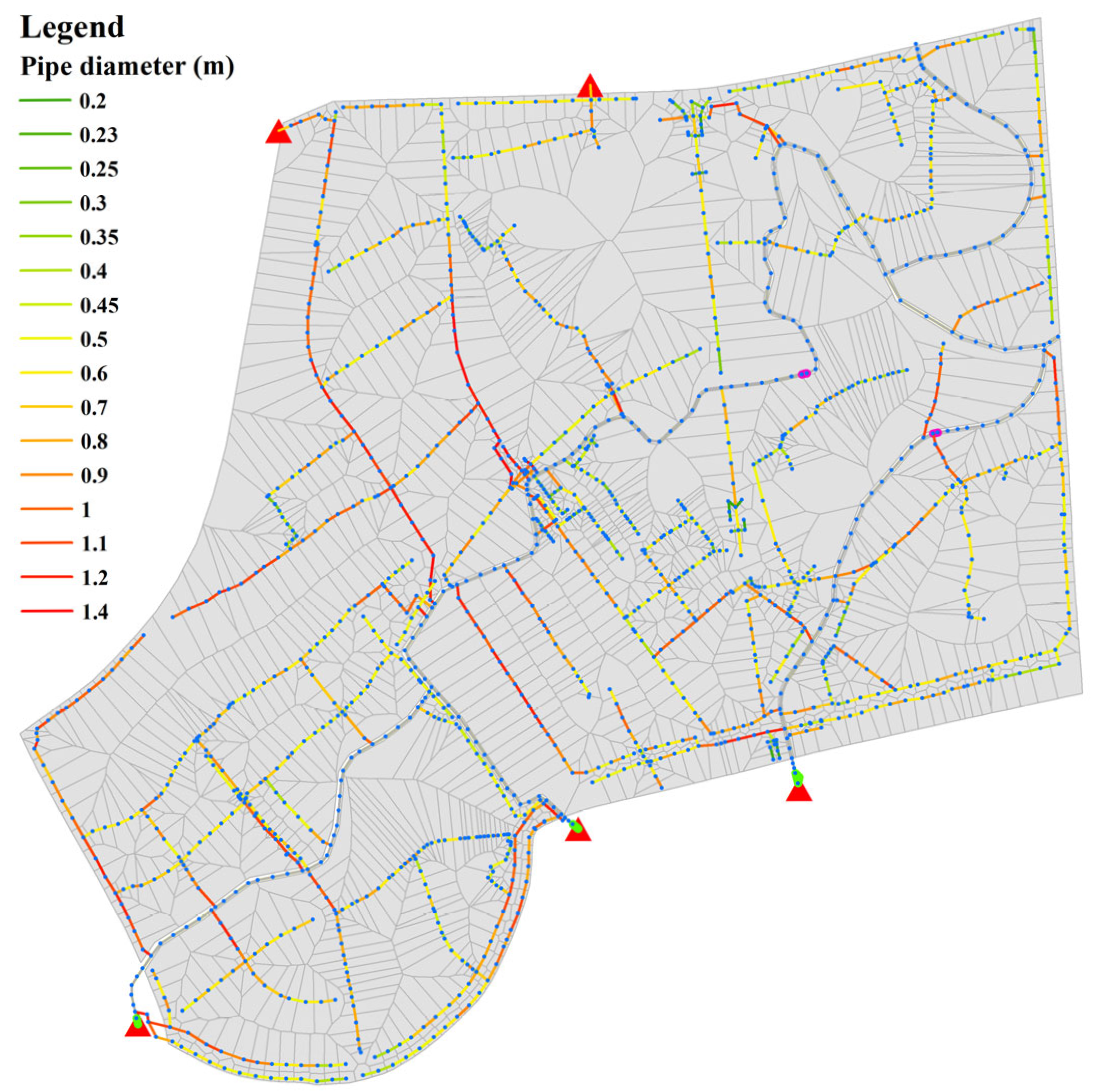
Taking the 5-year design storm as an example, among the 644 bottleneck pipes, 161 exhibited adverse slopes, all of which were corrected during the rehabilitation process. The spatial distribution of pipe diameters under the TOPSIS-optimal solution is shown in Figure 11. For the non-bottleneck pipes, some pipe diameters in the original network still did not conform to the standard commercial diameter series, such as 0.20 m and 0.23 m. After rehabilitation, the proportions of pipe diameters in the ranges of D ≤ 600 mm, 600 < D ≤ 1000 mm, and D ≥ 1000 mm were 59.2%, 31.5%, and 9.3%, respectively. Compared with the original pipe diameter distribution, the proportion of pipes with diameters greater than 600 mm increased significantly after rehabilitation.

This study further calculated the number of bottleneck pipes in the TOPSIS-optimal solutions under different return-period conditions (3-year, 5-year, 10-year, and 20-year). After rehabilitation, the proportions of bottleneck pipes were 23.63%, 25.35%, 24.94%, and 26.41%, respectively. Compared with the pre-rehabilitation condition, the numbers of bottleneck pipes were reduced by 34.91%, 32.46%, 37.76%, and 35.53%, respectively. These results indicate that the proposed optimization design model for stormwater pipe network rehabilitation can effectively reduce the number of pipes with insufficient drainage capacity.

4. Discussion

The results of this study demonstrate that integrating hydraulic diagnosis with multi-objective optimization provides a practical and physically interpretable framework for drainage network rehabilitation. In contrast to many previous studies, which either directly optimized pipe substitution and storage facilities or evaluated alternative algorithms without a prior hydraulic diagnosis of candidate pipes [9,10,12,13], the present study first identified bottleneck pipes through an improved bottleneck index and then used the diagnosed results to define the decision set for optimization. This diagnosis-driven strategy is more consistent with engineering practice, because rehabilitation is directed toward hydraulically critical pipes rather than being determined solely by an algorithmic search over a large decision space. It therefore provides a more targeted basis for rehabilitation design in old urban districts, where large-scale reconstruction is often constrained by cost, traffic disturbance, and limited construction space.

Another important finding is that the proportion of bottleneck pipes increased with storm return period but gradually approached saturation under larger return periods. This pattern suggests that the hydraulic behavior of the system is controlled by a relatively limited number of structurally and hydraulically critical conduits. Once these major bottlenecks become activated, further increases in rainfall intensity mainly aggravate surcharge and overflow at the already critical locations, rather than causing a proportional expansion in the number of newly critical pipes. A similar implication can be drawn from previous rehabilitation studies, which emphasized that system performance should be evaluated using drainage-network response variables such as overflow or flood consequences rather than rainfall input alone [8]. In this sense, the present results further support the argument that rehabilitation should focus on decisive hydraulic controls within the network rather than uniformly enlarging all pipes.

The optimization results also showed a clear trade-off between rehabilitation cost and drainage performance, which is consistent with earlier SWMM-based rehabilitation studies [9,10,12]. However, the comparison between the 1.2 m and 1.5 m maximum allowable rehabilitated pipe diameters revealed that further enlarging the upper pipe-diameter limit produced only limited reductions in total nodal overflow volume, while the rehabilitation cost increased in all tested scenarios. This indicates that system performance was not controlled solely by pipe diameter enlargement, but was also influenced by downstream boundary conditions, local topography, and the spatial distribution of bottleneck pipes. Once the dominant bottleneck sections had been relieved, additional increases in allowable diameter yielded only marginal hydraulic benefit. Similar findings have been reported in studies where pipe substitution alone did not necessarily result in proportional flood reduction, especially when system response was constrained by other structural or hydraulic factors [10,12,13]. Therefore, the superiority of the 1.2 m scheme in this study should be interpreted not simply as a result of lower cost, but also as evidence of diminishing marginal returns in pipe enlargement-based rehabilitation.

From the perspective of optimization efficiency, the proposed framework can also be interpreted as a hydraulically informed reduction in the search space. The difficulty of large decision spaces has been recognized as a major challenge in drainage rehabilitation optimization, and search-space reduction has recently been proposed as a way to improve computational efficiency and solution quality [11]. Compared with purely algorithmic reduction strategies, the present approach achieves a similar objective through hydraulic diagnosis by restricting the decision variables to bottleneck pipes and pipes directly connected to the river. This not only reduces the number of candidate variables but also preserves a clear engineering rationale for why these pipes are included in the optimization. Such an approach is particularly useful for large existing drainage networks, where full-network optimization may become computationally burdensome and difficult to interpret from a practical decision-making perspective.

The present framework should also be understood in the context of other rehabilitation strategies reported in the literature. Several studies have shown that integrating pipe replacement with storm tanks, storage facilities, or LID/BMP measures can further enhance flood mitigation performance [12,13,16]. Other studies have demonstrated that risk-based or resilience-based rehabilitation frameworks may provide more robust solutions when rainfall uncertainty, blockage scenarios, or flood damage are explicitly incorporated into the optimization process. In comparison, the current study focused on deterministic design-storm conditions and pipe-network rehabilitation only. This simplification is reasonable for the target application, namely old urban districts where large-scale implementation of storm tanks or green infrastructure is often impractical because of limited land availability and high retrofitting costs. Therefore, the proposed method does not replace integrated gray–green or uncertainty-based approaches, but rather complements them by offering a more directly implementable diagnosis-driven solution for densely built urban areas.

The calibration of the hydrodynamic model using a single rainfall event represents an important source of uncertainty in this study. Because the available high-quality monitoring data were limited, the calibrated parameter set could not be further validated against rainfall events with different magnitudes, durations, and temporal patterns. Consequently, uncertainties in the hydrological and hydraulic parameters may propagate to the simulated nodal hydraulic heads and pipe filling ratios, thereby affecting the identified number and spatial distribution of bottleneck pipes. These uncertainties may further influence the selection of candidate pipes for rehabilitation and the quantitative optimization results, including rehabilitation cost and total nodal overflow volume.

The generalizability of the case-study findings may also be affected by catchment topography and downstream boundary conditions. The Sanjie River catchment is a coastal intermontane basin, where local topographic variation, river water levels, tidal effects, and backwater conditions can strongly influence drainage system performance. Therefore, the conclusion that further pipe enlargement provides only limited additional hydraulic benefits should be interpreted primarily in the context of the present study area. In flat urban catchments, limited hydraulic gradients and downstream backwater effects may play a more dominant role, whereas in steep catchments, pipe slope and flow velocity constraints may become more important. As a result, the relative effectiveness of pipe enlargement and the spatial distribution of bottleneck pipes may differ among regions.

These limitations mainly affect the quantitative results obtained for the present case study rather than the general formulation of the proposed diagnosis-driven rehabilitation framework. Nevertheless, the engineering reliability and transferability of the results depend on the accuracy of the underlying hydrodynamic model and the local topographic, rainfall, and boundary conditions. In addition, the current framework was established under deterministic design-storm conditions and did not explicitly consider rainfall uncertainty, blockage scenarios, or climate-change-driven variability, all of which may influence rehabilitation decisions [15,26,27]. Only pipe-based rehabilitation was considered in the optimization. In other urban contexts, especially where land is available or where source-control measures can be effectively implemented, combined strategies involving pipe replacement, storage facilities, and LID/BMP measures may achieve better long-term performance [12,16]. Moreover, sewer rehabilitation may interact with surrounding hydrological conditions in complex ways, and previous studies have shown that rehabilitation can alter groundwater behavior in low-lying coastal urban areas [14]. Future studies should therefore use multiple rainfall events covering different storm magnitudes and temporal patterns for model calibration and validation, and further test the proposed framework in drainage networks with different terrain characteristics, hydrological conditions, and rehabilitation strategies.

5. Conclusions

This study proposed a multi-objective hydraulic optimization framework for the rehabilitation of urban stormwater drainage networks by coupling SWMM simulation, an improved bottleneck index method, and the NSGA-III algorithm. The proposed framework enables the effective identification of bottleneck pipes and provides a practical basis for selecting rehabilitation schemes for existing drainage systems.

The results showed that the proportion of bottleneck pipes increased with the design storm return period, while the rate of increase gradually diminished under larger return periods. The optimization results also demonstrated a clear trade-off between rehabilitation cost and drainage performance. Simply increasing the maximum allowable rehabilitated pipe diameter did not lead to substantial additional improvement in system performance.

Overall, the proposed framework provides a systematic and engineering-oriented approach for diagnosing and rehabilitating existing urban stormwater drainage networks, and can support decision-making for cost-effective rehabilitation design. The proposed framework is particularly suitable for old urban districts where complete network reconstruction is difficult to implement and cost-effective rehabilitation is required.

In practical applications, the proposed framework can be further developed into a GIS- or SWMM-based decision-support tool for municipal engineers, providing bottleneck pipe maps, candidate rehabilitation pipe lists, and cost–performance comparison tables to support rapid screening and comparison of drainage network rehabilitation schemes.

References

1. Zhang, Y.; Wang, E.; Gong, Y. A structural optimization of urban drainage systems: An optimization approach for mitigating urban floods. Water 2024, 16, 1696. [Google Scholar] [CrossRef]
2. Heydari Mofrad, H.; Yazdi, J. An enhanced multi-objective evolutionary algorithm for the rehabilitation of urban drainage systems. Eng. Optim. 2022, 54, 349–367. [Google Scholar]
3. Xu, C.; Tang, T.; Jia, H.; Xu, M.; Xu, T.; Liu, Z.; Long, Y.; Zhang, R. Benefits of coupled green and grey infrastructure systems: Evidence based on analytic hierarchy process and life cycle costing. Resour. Conserv. Recycl. 2019, 151, 104478. [Google Scholar] [CrossRef]
4. Gao, Z.; Zhang, Q.H.; Xie, Y.D.; Wang, Q.; Dzakpasu, M.; Xiong, J.Q.; Wang, X.C. A novel multi-objective optimization framework for urban green-gray infrastructure implementation under impacts of climate change. Sci. Total Environ. 2022, 825, 153954. [Google Scholar] [CrossRef] [PubMed]
5. Zhang, W.; Li, J.; Chen, Y.; Li, Y. A surrogate-based optimization design and uncertainty analysis for urban flood mitigation. Water Resour. Manag. 2019, 33, 4201–4214. [Google Scholar] [CrossRef]
6. Shu, X.; Ye, C.; Xu, Z.; Liao, R.; Song, P.; Zhang, S. An enhanced framework for assessing pluvial flooding risk with integrated dynamic population vulnerability at urban scale. Remote Sens. 2025, 17, 654. [Google Scholar] [CrossRef]
7. Wang, F.Z.; Xu, B.H.; Li, C.M.; Qiu, J.L.; Liu, C.; Xu, L.Z. Design of large closed loop control structure for urban drainage systems in the whole optimizing running process. Appl. Mech. Mater. 2013, 409, 1012–1016. [Google Scholar] [CrossRef]
8. Gaudio, R.; Penna, N.; Viteritti, V. A combined methodology for the hydraulic rehabilitation of urban drainage networks. Urban Water J. 2016, 13, 644–656. [Google Scholar]
9. Yazdi, J.; Mohammadiun, S.; Sadiq, R.; Neyshabouri, S.S.; Gharahbagh, A.A. Assessment of different moeas for rehabilitation evaluation of urban stormwater drainage systems–case study: Eastern catchment of tehran. J. Hydro-Environ. Res. 2018, 21, 76–85. [Google Scholar] [CrossRef]
10. Yazdi, J.; Yoo, D.G.; Kim, J.H. Comparative study of multi-objective evolutionary algorithms for hydraulic rehabilitation of urban drainage networks. Urban Water J. 2017, 14, 483–492. [Google Scholar] [CrossRef]
11. Ngamalieu-Nengoue, U.A.; Iglesias-Rey, P.L.; Martínez-Solano, F.J.; Mora-Meliá, D. Iterative search space reduction (issr) for optimal flood control in urban drainage networks. Water 2024, 16, 458. [Google Scholar] [CrossRef]
12. Ngamalieu-Nengoue, U.A.; Martínez-Solano, F.J.; Iglesias-Rey, P.L.; Mora-Meliá, D. Multi-objective optimization for urban drainage or sewer networks rehabilitation through pipes substitution and storage tanks installation. Water 2019, 11, 935. [Google Scholar] [CrossRef]
13. Iglesias-Rey, P.L.; Martínez-Solano, F.J.; Saldarriaga, J.G.; Navarro-Planas, V.R. Pseudo-genetic model optimization for rehabilitation of urban storm-water drainage networks. Procedia Eng. 2017, 186, 617–625. [Google Scholar] [CrossRef]
14. Su, X.; Liu, T.; Beheshti, M.; Prigiobbe, V. Relationship between infiltration, sewer rehabilitation, and groundwater flooding in coastal urban areas. Environ. Sci. Pollut. Res. Int. 2020, 27, 14288–14298. [Google Scholar] [PubMed]
15. Yazdi, J. Improving urban drainage systems resiliency against unexpected blockages: A probabilistic approach. Water Resour. Manag. 2018, 32, 4561–4573. [Google Scholar] [CrossRef]
16. Azari, B.; Tabesh, M. Urban storm water drainage system optimization using a sustainability index and lid/bmps. Sustain. Cities Soc. 2022, 76, 103500. [Google Scholar] [CrossRef]
17. Dong, L.; Li, T.; Qian, J. Application of hydraulic performance index in up-to-standard reconstruction of drainage system. China Water Wastewater 2011, 27, 96–100. [Google Scholar]
18. Tang, L.L.; Hu, J.C.; Liu, Z.; Yang, Z.G.; Li, Q.Q. Bottleneck analysis and reform evaluation of urban underground drainage pipe network based on swmm. China Water Wastewater 2018, 34, 112–117. [Google Scholar]
19. Rossman, L.A.; Simon, M.A. Storm Water Management Model User’s Manual Version 5.2; Center for Environmental Solutions and Emergency Response Office of Research and Development, United States Environmental Protection Agency: Washington, DC, USA, 2022. [Google Scholar]
20. Bakhshipour, A.E.; Dittmer, U.; Haghighi, A.; Nowak, W. Hybrid green-blue-gray decentralized urban drainage systems design, a simulation-optimization framework. J. Environ. Manag. 2019, 249, 109364. [Google Scholar] [CrossRef]
21. Rossman, L.A. Storm Water Management Model Reference Manual Volume II—Hydraulics; US Environmental Protection Agency: Washington, DC, USA, 2017. [Google Scholar]
22. Feng, Y.; Huang, X.; Ma, D. A comparative analysis of auto-calibration strategies for the urban hydrologic model. Hydrol. Res. 2025, 56, 636–654. [Google Scholar] [CrossRef]
23. Ding, X.; Liao, W.; Lei, X.; Wang, H.; Yang, J.; Wang, H. Assessment of the impact of climate change on urban flooding: A case study of Beijing, China. J. Water Clim. Change 2022, 13, 3692–3715. [Google Scholar] [CrossRef]
24. Deb, K.; Jain, H. An evolutionary many-objective optimization algorithm using reference-point-based nondominated sorting approach, part i: Solving problems with box constraints. IEEE Trans. Evol. Comput. 2014, 18, 577–601. [Google Scholar] [CrossRef]
25. Hwang, C.; Yoon, K. Methods for multiple attribute decision making. In Multiple Attribute Decision Making: Methods and Applications a State-of-the-Art Survey; Springer: Berlin/Heidelberg, Germany, 1981; pp. 58–191. [Google Scholar]
26. Yazdi, J.; Heydari Mofrad, H.; Heydari Mofrad, M. Development of a risk-based optimization approach to improve the performance of urban drainage systems. Hydrol. Sci. J. 2022, 67, 689–702. [Google Scholar] [CrossRef]
27. Yazdi, J. Rehabilitation of urban drainage systems using a resilience-based approach. Water Resour. Manag. 2018, 32, 721–734. [Google Scholar] [CrossRef]
Figure 1. The proposed framework.
Water 18 01683 g001
Figure 2. Distribution map of the model in Sanjie River Basin.
Water 18 01683 g002
Figure 3. Observed rainfall hyetograph.
Water 18 01683 g003
Figure 4. Schematic diagram of the slope relationship for a bottleneck pipe (hydraulic gradient greater than pipe slope).
Water 18 01683 g004
Figure 5. Schematic diagram of the slope relationship for a bottleneck pipe (hydraulic gradient less than pipe slope).
Water 18 01683 g005
Figure 6. Simulated water depths of stormwater manholes: (a) J1; (b) J2; (c) J3.
Water 18 01683 g006
Figure 7. Variation in the proportion of bottleneck pipes under different return periods.
Water 18 01683 g007
Figure 8. Distribution map of bottleneck pipes under different return periods.
Water 18 01683 g008aWater 18 01683 g008b
Figure 9. Multi-objective optimization results under a maximum allowable diameter of 1.2 m for post-retrofitting pipes: (a) 3-year; (b) 5-year; (c) 10-year; (d) 20-year.
Water 18 01683 g009
Figure 10. Multi-objective optimization results under a maximum allowable diameter of 1.5 m for post-retrofitting pipes: (a) 3-year; (b) 5-year; (c) 10-year; (d) 20-year.
Water 18 01683 g010
Figure 11. Spatial distribution of pipe diameters corresponding to the TOPSIS-optimal solution.
Water 18 01683 g011