High-Frequency Dissolved Oxygen Dynamics Reveal a Site-Specific Threshold for Hypoxia-Related Oxygen Stress in a Shallow Eutrophic Lake

Abstract

High-frequency monitoring provides a practical approach for detecting short-term oxygen instability and pre-transition stress accumulation in eutrophic shallow lakes. In this study, dissolved oxygen (DO), pH, water temperature, and electrical conductivity (EC) were monitored at 5 min intervals in a restored shallow urban lake in Wuhan, China. A total of 112,896 synchronized observations from 392 complete daily profiles were analyzed to characterize diel physicochemical dynamics, identify a site-specific DO threshold, and evaluate process-based early-warning indicators. DO and pH showed pronounced synchronized diel oscillations; whereas, temperature mainly reflected seasonal background variation and EC showed weaker diel regularity. Correlation analysis and PCA indicated that DO and pH represented the dominant metabolic gradient, with DO serving as the most responsive indicator of oxygen instability. Piecewise logistic regression identified a site-specific DO threshold of 3.62 mg L⁻¹ associated with persistent hypoxia-related oxygen-stress states. During the August 2021 transition period, low-oxygen duration increased rapidly, oxygen-stress exposure intensified, and daytime recovery rate declined, indicating progressive oxygen-stress accumulation and weakened recovery capacity. These results show that high-frequency DO dynamics can provide early-warning information on persistent hypoxia-related oxygen stress, although the identified threshold should be interpreted as site-specific rather than universal.

1. Introduction

Eutrophic shallow lakes are increasingly affected by rapid metabolic fluctuations, nonlinear transitions toward persistent low-oxygen conditions, and short-lived ecological stress events under the combined influence of eutrophication and climate warming. However, most ecological assessment frameworks still rely on weekly or monthly observations and therefore implicitly assume gradual ecosystem change. Traditional water-quality assessment commonly relies on integrated water-quality indices derived from a limited set of physicochemical variables and infrequent observations, which may fail to capture rapid ecological processes and short-term ecosystem instability [1]. This mismatch limits the ability to detect statistical hypoxia thresholds and early instability in eutrophic shallow lakes. Conventional low-frequency monitoring often fails to capture diel fluctuations in dissolved oxygen (DO) and pH, thereby underestimating the intensity, duration, and recurrence of hypoxic stress events [2]. As a result, ecological deterioration may remain undetected until substantial degradation has already occurred, reducing opportunities for timely intervention to mitigate hypoxia-related oxygen stress [3,4,5].

High-frequency monitoring provides an opportunity to move beyond state-based assessments and to develop process-oriented indicators that resolve ecosystem metabolism and short-term instability [6,7]. Sensor-based high-frequency records can capture short-lived events, diel fluctuations, abrupt anomalies, and recovery processes that are often missed by conventional grab sampling, making them valuable for water-quality assessment and practical management applications [8]. Such datasets are particularly useful for dissolved oxygen analysis because DO responds rapidly to photosynthesis, respiration, temperature variation, hydrodynamic mixing, and short-term external forcing [9,10]. However, reliable interpretation of high-frequency datasets requires careful sensor deployment, calibration, maintenance, quality control, and data screening to avoid overinterpreting sensor artifacts as ecological signals [11]. In the context of early warning, indicator performance depends strongly on sampling frequency and data continuity, because pre-transition signals may occur over short temporal windows before persistent deterioration becomes evident [12]. Therefore, integrating high-frequency monitoring with process-based indicators provides a practical pathway for detecting oxygen-stress accumulation in shallow eutrophic lakes.

In eutrophic shallow lakes, DO and pH exhibit pronounced diel oscillations driven by the balance between photosynthesis and community respiration [13,14]. These cycles repeatedly generate alternating periods of nocturnal oxygen depletion and daytime recovery, suggesting that oxygen-stress exposure may accumulate through recurrent daily metabolic interruptions rather than through isolated disturbance events [15,16]. In this study, DO, pH, water temperature, and electrical conductivity (EC) were selected as core high-frequency physicochemical variables because they provide complementary information on short-term lake metabolism and oxygen instability. DO directly reflects ecosystem metabolic balance and oxygen stress; whereas, pH serves as an indicator of biological production and carbon dynamics. Water temperature regulates metabolic intensity and oxygen demand, while EC reflects hydrochemical background conditions and potential external influences. Together, these variables characterize different aspects of ecosystem functioning and instability. When monitored at high frequency, they enable the quantification of nocturnal oxygen depletion, daytime recovery capacity, diel amplitude, and threshold-approaching trajectories that are typically overlooked by conventional monitoring programs.

Ecological deterioration in eutrophic shallow lakes may therefore emerge not from a single abrupt disturbance but from the cumulative effect of many small daily metabolic interruptions, including recurrent nocturnal oxygen depletion, incomplete daytime recovery, and repeated metabolic imbalances. Ignoring these accumulation processes may reduce the ability of conventional assessment and prediction frameworks to detect early warning signals of a transition toward persistent low-oxygen conditions. Recent studies have emphasized the importance of identifying early-warning signals prior to regime shifts in aquatic ecosystems, although translating theoretical indicators into practical monitoring tools remains challenging [17]. To address this gap, this study developed a high-frequency ecological indicator framework for identifying metabolic instability, site-specific statistical hypoxia thresholds, and an approaching transition toward persistent low-oxygen conditions in a eutrophic shallow lake. Using 112,896 observations collected at 5 min intervals over 392 monitoring days, we integrated diel metabolic analysis, nonlinear threshold detection, principal component analysis (PCA), and partial least squares structural equation modeling (PLS-SEM) to investigate the ecological roles of DO, pH, temperature, and EC in describing ecosystem metabolism and instability. Monthly total phosphorus measurements were additionally incorporated into the exploratory PLS-SEM analysis as a trophic-pressure background variable to link nutrient conditions with high-frequency DO-derived oxygen-stress indicators. Specifically, this study aimed to (i) characterize the diel and seasonal dynamics of DO, pH, temperature, and EC using high-frequency monitoring data; (ii) identify a site-specific DO threshold associated with persistent hypoxia-related oxygen-stress states; and (iii) evaluate low-oxygen duration, cumulative oxygen deficit, and daytime recovery rate as process-based early-warning indicators of oxygen-stress accumulation in a shallow eutrophic lake.

2. Materials and Methods

2.1. Study Area

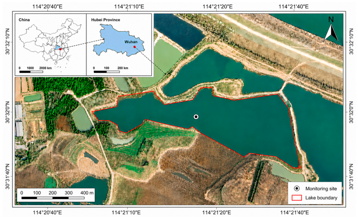
This study was conducted in a shallow lake, Lijiajiao Lake, located in Wuhan City, Hubei Province, China (Figure 1), centered at approximately 30°37′ N, 114°04′ E. The lake is a typical shallow freshwater lake on the Jianghan Plain of Hubei Province, with a surface area of about 0.5 km² and an average depth of 1.5–2.0 m. The lake lacks major natural inflow or outflow rivers. It therefore functions as a relatively enclosed hydrological system with low water-exchange capacity, a typical feature of small urban and peri-urban lakes that increases their vulnerability to eutrophication [18]. However, this hydrological setting does not imply that external inputs or short-term external forcing were negligible. Rainfall, urban runoff, wind-driven mixing, water-level changes, and episodic hydrological disturbances were not explicitly quantified in this study and were therefore considered as potential sources of uncertainty. Due to its long history of eutrophication, it is a pilot site under China’s one-lake-one-policy restoration framework during this research, which aims to improve lake water quality through ecosystem restoration.

2.2. Data Collection

2.2.1. Automatic Monitoring of High-Frequency Physicochemical Variables

A floating-platform automatic monitoring station was self-assembled and equipped with multi-parameter sensors for continuous observation in Lijiajiao Lake. The monitoring system included pH sensors, dissolved oxygen sensors with temperature measurement, electrical conductivity sensors, a 3 m support pole with sensor-fixing brackets and submerged pipes, sensor floats, and protective boxes for the data-acquisition and power-supply systems. The sensors were fixed in submerged pipes attached to the 3 m support pole and installed at approximately 0.5 m below the water surface, consistent with the depth used for manual TP sampling. Given the average lake depth of 1.5–2.0 m, this fixed monitoring depth represented near-surface water conditions at the monitoring site rather than vertically integrated whole-lake oxygen conditions. The monitoring system continuously measured dissolved oxygen (DO), pH, water temperature, and electrical conductivity (EC) at approximately 5 min intervals from 1 August 2020 to 31 December 2021. The main components and available sensor characteristics recorded in the equipment documentation are summarized in Supplementary Table S1. Complete records of sensor brand, model, manufacturer address, resolution, and routine calibration frequency were not available from the archived equipment documentation; therefore, only documented sensor characteristics are reported.

During the monitoring period, the sensors were inspected and maintained according to field-operation records. Maintenance included sensor cleaning, removal of attached particles or biofilms, inspection of probe surfaces, and functional checks when abnormal readings, power interruption, or sensor instability were detected. Potential sensor drift or biofouling was assessed by examining abrupt shifts, prolonged flat-line values, progressive divergence among the three parallel channels, and inconsistencies with adjacent 5 min observations. Because complete routine calibration-frequency records were unavailable, potential sensor drift and biofouling effects were controlled using maintenance-log screening, multi-channel consistency checks, temporal-continuity inspection, and complete-day filtering. Records collected during identifiable cleaning, calibration, repair, power interruption, or platform maintenance were excluded before daily profile construction. The detailed data-screening rules are described in Section 2.3, and the excluded periods are summarized in Supplementary Table S2.

2.2.2. Manual Sampling of Total Phosphorus (TP) and Treatment

Total phosphorus (TP) was monitored via monthly manual sampling at the same location as the automatic monitoring station to ensure comparability of results. TP was included as a representative monthly nutrient-pressure indicator rather than as a high-frequency variable. It was used to provide a trophic-pressure background for the exploratory PLS-SEM analysis and to examine whether monthly nutrient conditions were associated with DO-related oxygen-stress indicators. Surface water was collected at a depth of 0.5 m into pre-acid-washed polyethylene bottles (500 mL). Samples were acidified to pH < 2, stored at 4 °C, and analyzed in the laboratory. TP concentrations were determined using the molybdate spectrophotometric method (GB/T 11893-1989), consistent with widely used colorimetric methods [19]. Quality control procedures included field duplicates (relative deviation ≤10%), field blanks, and laboratory control samples (error ≤±5%), in accordance with QA/QC guidelines for nutrient analysis in freshwater systems [20].

2.3. Data Preprocessing and Quality Control

Raw high-frequency monitoring records were screened and reorganized before analysis. The original dataset was recorded by a multi-parameter sensor at approximately 5 min intervals and contained three parallel channels for each variable, including water temperature, pH, electrical conductivity (EC), and dissolved oxygen (DO). For each timestamp, channel-specific readings were first checked and then averaged to obtain one representative value for each variable.

The QA/QC procedure included range checks, timestamp checks, sensor-artifact screening, maintenance-related data exclusion, and complete-day screening. Values were treated as invalid if they were missing, non-numeric, negative, or outside physically plausible and instrument-consistent ranges: water temperature, 0–45 °C; pH, 0–14; EC, 0–5 mS cm⁻¹; and DO, 0–25 mg L⁻¹. Logical errors, including duplicated timestamps, non-chronological timestamps, and irregular timestamp intervals, were also removed [21].

Potential sensor-related artifacts and maintenance-related records were further screened before daily profile construction. Because complete routine calibration-frequency records were unavailable, potential sensor drift and biofouling effects were evaluated using maintenance-log screening, internal consistency checks among the three parallel channels, and temporal-continuity inspection. Records obtained during identifiable maintenance operations, such as sensor cleaning, calibration, power interruption, probe replacement, or platform maintenance, were treated as invalid and removed. Abnormal sensor segments were flagged when they showed long flat-line values, abrupt step changes inconsistent with adjacent observations, progressive divergence among parallel channels, or isolated spikes that were inconsistent with neighboring 5 min observations and physically plausible short-term variability. Flagged records were manually reviewed according to the above criteria and removed only when they could not be reasonably interpreted as natural short-term variability.

Because the monitoring interval was 5 min, a complete 24 h daily profile was expected to contain 288 observations per variable. To minimize bias caused by missing values or maintenance-related interruptions in high-frequency sensor records, strict filtering and temporal alignment procedures were applied before daily scale analysis [22]. This complete-day criterion was required because the main indicators used in this study, including daily minimum DO, day–night DO difference, below-threshold duration, cumulative oxygen deficit, and diel variation patterns, depend on full daytime and nighttime coverage. Therefore, no gap filling or interpolation was applied. If the removal of maintenance-related or abnormal records caused any variable to have fewer than 288 valid observations within a 24 h period, the entire daily profile was excluded from daily scale analyses. The excluded periods and reasons for exclusion are summarized in Supplementary Table S2.

After QA/QC filtering, the daily matrices of DO, pH, temperature, and EC were synchronized by date. Only dates with complete 288-point daily profiles for all four variables were retained for subsequent four-parameter analyses. The final synchronized dataset contained 392 complete daily profiles, corresponding to 112,896 synchronized 5 min observations for each variable.

2.4. Analytical Methods

2.4.1. Analysis of Diel and Seasonal Variations in High-Frequency Physicochemical Variables

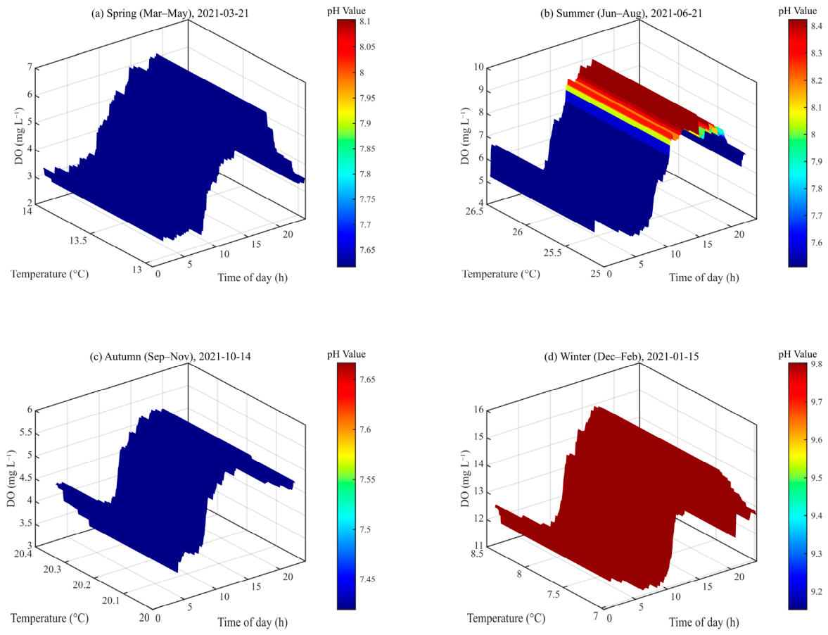
The diel fluctuations and seasonal variability in the four high-frequency physicochemical variables, i.e., DO, pH, temperature, and EC, were characterized using high-frequency data analysis, which provides essential insights into diel ecological processes that traditional low-frequency sampling cannot capture [9,23]. The four parameters were categorized by day and plotted as long-term diel fluctuation diagrams to identify short-term ecological stress events [24,25]. A DO heatmap (“time × date”) was constructed to capture seasonal drift and low-oxygen zone formation. For each season, a representative day was selected to generate a 3D surface diagram illustrating the diel coupling among Temp, pH, and DO. Similar approaches have been widely used in studies of lake metabolism and hypoxia [14,26].

2.4.2. Identification of Key Ecological Indicators

Relationships among DO, pH, temperature, and EC were evaluated using Spearman’s rank correlation, with Pearson’s correlation applied as a robustness check. In addition, the dataset was divided into four seasons, and diel variation curves were compared across seasons to assess each parameter’s responsiveness to short-term ecosystem processes. Seasonal diel patterns provide insight into how temperature, primary productivity, and ecosystem metabolism influence environmental dynamics [27,28]. Parameters exhibiting strong associations with other environmental variables, together with pronounced diel and seasonal variability, were considered more suitable indicators of ecosystem-state fluctuations and oxygen-stress escalations.

2.4.3. Definition of Hypoxia-Related Oxygen-Stress State and DO Threshold Detection

A hypoxia-related oxygen-stress state was defined to characterize persistent low-oxygen conditions in the high-frequency dissolved oxygen (DO) record. This definition was intended to identify periods during which DO dynamics indicated sustained oxygen stress, as reflected by prolonged low DO, cumulative oxygen deficit, and insufficient daytime recovery. Such process-based indicators are useful for detecting early changes in aquatic systems before visible ecological consequences become apparent. Accordingly, the binary response variable was used to distinguish hypoxia-related oxygen-stress conditions from non-stress conditions in the DO record.

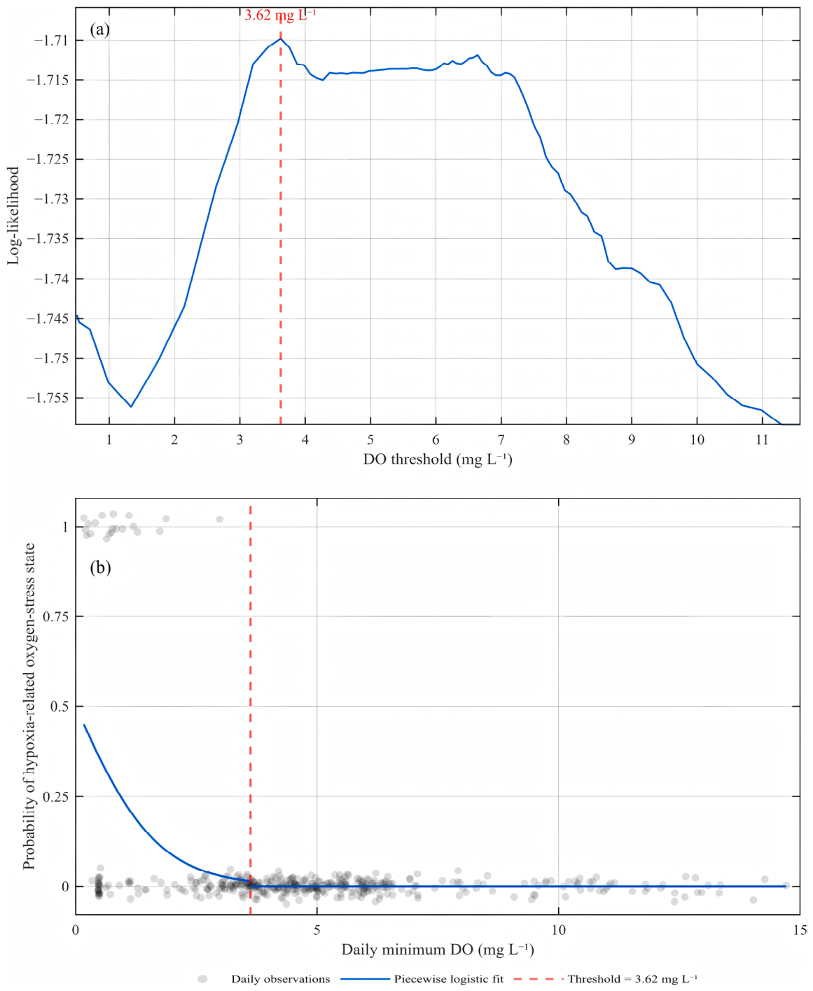
A threshold analysis based on piecewise logistic regression was then applied to the high-frequency DO dataset to identify the DO level at which oxygen-related system states showed a marked statistical transition. Candidate thresholds were generated from the empirical distribution of observed DO values. For each candidate threshold, the dataset was divided into two subsets according to whether DO values were below or above the candidate value, and logistic regression models were fitted separately for the two subsets. The total log-likelihood of the two fitted models was calculated, and the optimal threshold was defined as the candidate value that maximized the total log-likelihood. This value represented the most pronounced statistical transition in the relationship between DO and hypoxia-related oxygen-stress conditions. To ensure model stability, candidate thresholds were excluded when they resulted in insufficient sample size, single-category outcomes within either subset, or non-convergent model fits. The remaining valid thresholds were used to construct a threshold–log-likelihood curve, from which the DO-based transition point was identified. Threshold-based and likelihood-based approaches have been widely applied to detect nonlinear ecological transitions, regime shifts, and oxygen-related stress responses in aquatic ecosystems [3,29,30,31]. In the present study, this approach was used specifically to identify a site-specific DO threshold associated with persistent hypoxia-related oxygen stress.

To evaluate the stability of the identified DO threshold, a sensitivity analysis was conducted using alternative definitions of the hypoxia-related oxygen-stress state. In addition to the baseline definition used in the main analysis, oxygen-stress states were reclassified using alternative criteria based on daily low-oxygen duration and cumulative oxygen deficit. Specifically, low-oxygen duration criteria of >1, >2, and >4 h d⁻¹ below the identified DO threshold were tested, and OSEI-based criteria using the 75th and 80th percentiles were also applied. For each alternative classification, the same threshold–log-likelihood search procedure was repeated, and the resulting threshold was compared with the baseline threshold of 3.62 mg L⁻¹. The results of the sensitivity analysis are presented in Table S3.

The identified DO threshold was further used to quantify oxygen-stress accumulation and recovery dynamics during the transition period. Three threshold-based indicators were calculated: low-oxygen duration, oxygen-stress exposure index (OSEI), and daytime recovery rate. Low-oxygen duration was calculated as the cumulative daily duration during which DO remained below the identified threshold. OSEI was calculated as the cumulative oxygen deficit below the threshold:

OSEI = Σ(DO_th − DO_i) × Δt, for DO_i < DO_th,

where DO_th represents the identified DO threshold, DO_i represents each 5 min DO observation, and Δt is the sampling interval expressed in hours. This metric integrates both the intensity and duration of oxygen stress. Daytime recovery rate was calculated as the mean positive 5 min DO increment during daytime periods (06:00–18:00), converted to an hourly rate (mg L⁻¹ h⁻¹). Temporal changes in these indicators were used to evaluate the progression of oxygen stress and recovery capacity before and after the onset of persistent low-oxygen conditions. All analyses were performed in MATLAB R2024a.

Because independent biological-response observations were not available at the same temporal resolution, the identified threshold was interpreted as a site-specific DO-based early-warning threshold for persistent hypoxia-related oxygen stress, rather than as a universal ecological threshold or a threshold of confirmed biological damage.

2.4.4. PCA Composite Evaluation Model

PCA was used to identify the dominant environmental gradients underlying high-frequency variability in DO, pH, temperature, and EC. Loading structures of retained components were used to evaluate the relative contributions of environmental indicators to lake metabolic dynamics and ecological variability. Composite indicator weights were subsequently calculated based on absolute loadings weighted by the variance explained by each principal component. PCA and composite weighting were conducted in MATLAB R2024a.

2.4.5. Exploratory PLS-SEM Analysis Based on PCA-Identified Latent Structure

To further examine whether the observed variables were consistent with the hypothesized pathway linking nutrient pressure, DO Condition, and persistent hypoxia-related oxygen-stress states, an exploratory partial least squares structural equation modeling (PLS-SEM) analysis was conducted. This analysis was not intended to establish strict causal relationships, but rather to evaluate the association structure among monthly nutrient conditions, DO dynamics, and oxygen-stress states [32,33].

The PLS-SEM model included three latent variables: Water_Quality, DO_Condition, and oxygen-stress state. Water_Quality was represented by TP and pH_above8_ratio. In this construct, TP was used to represent monthly nutrient-pressure background; whereas, pH_above8_ratio represented pH-related metabolic conditions aggregated from high-frequency observations. DO_Condition was represented by DO_mean, DO_below3.62_ratio, DO_std, and DO_daynight_diff, reflecting overall oxygen level, below-threshold oxygen exposure, oxygen variability, and diel oxygen recovery amplitude. Oxygen_Stress_State was represented by the binary indicator of persistent hypoxia-related oxygen-stress state. Reflective measurement models were specified for all constructs, and path coefficients and indicator loadings were used to evaluate relationships among variables. High-frequency DO and pH observations were aggregated into monthly metrics to match the monthly TP measurements. The definitions and ecological interpretations of the variables used in the exploratory PLS-SEM model are summarized in

Table 1. Definitions of variables used in the exploratory PLS-SEM model.

Variable	Calculation/Coding	Ecological Interpretation
TP	Monthly total phosphorus concentration	Monthly nutrient pressure indicator
pH_above8_ratio	Proportion of 5 min pH observations > 8 within each month	Proxy for enhanced photosynthetic activity and carbonate-related pH elevation
DO_mean	Monthly Mean DO concentration	Overall monthly oxygen condition
DO_below3.62_ratio	Proportion of 5 min DO observations < 3.62 mg L−1 within each month	Frequency of low-oxygen exposure below the identified site-specific DO threshold
DO_std	Monthly standard deviation of DO	Monthly oxygen variability
DO_daynight_diff	Monthly mean difference between daytime DO and nighttime DO	Diel oxygen recovery amplitude
Oxygen_Stress_State	0 = non-stress condition; 1 = persistent hypoxia-related oxygen-stress state	Process-based early-warning indicator of persistent oxygen stress, not confirmed biological damage

. Given the limited sample size (n = 12), the analysis was intended primarily to examine hypothesized ecological pathways rather than provide strict inferential tests [34,35]. The model was estimated using MATLAB R2024a. To assess the reliability and convergent validity of the exploratory measurement model, Cronbach’s α, composite reliability (CR), and average variance extracted (AVE) were calculated for the multi-indicator constructs. Because some indicators had opposite ecological directions, standardized indicators and outer loadings were direction-adjusted before calculating these diagnostics. Oxygen-stress state was specified as a single-indicator construct; therefore, Cronbach’s α, CR, and AVE were not applicable to this construct. Given the limited monthly sample size, these diagnostics were interpreted as exploratory rather than confirmatory evidence.

3. Results

3.1. Diel and Seasonal Variations in High-Frequency Physicochemical Variables

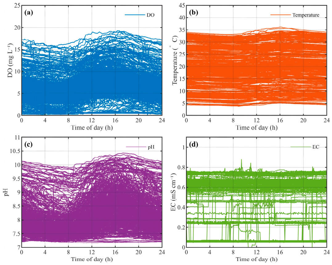
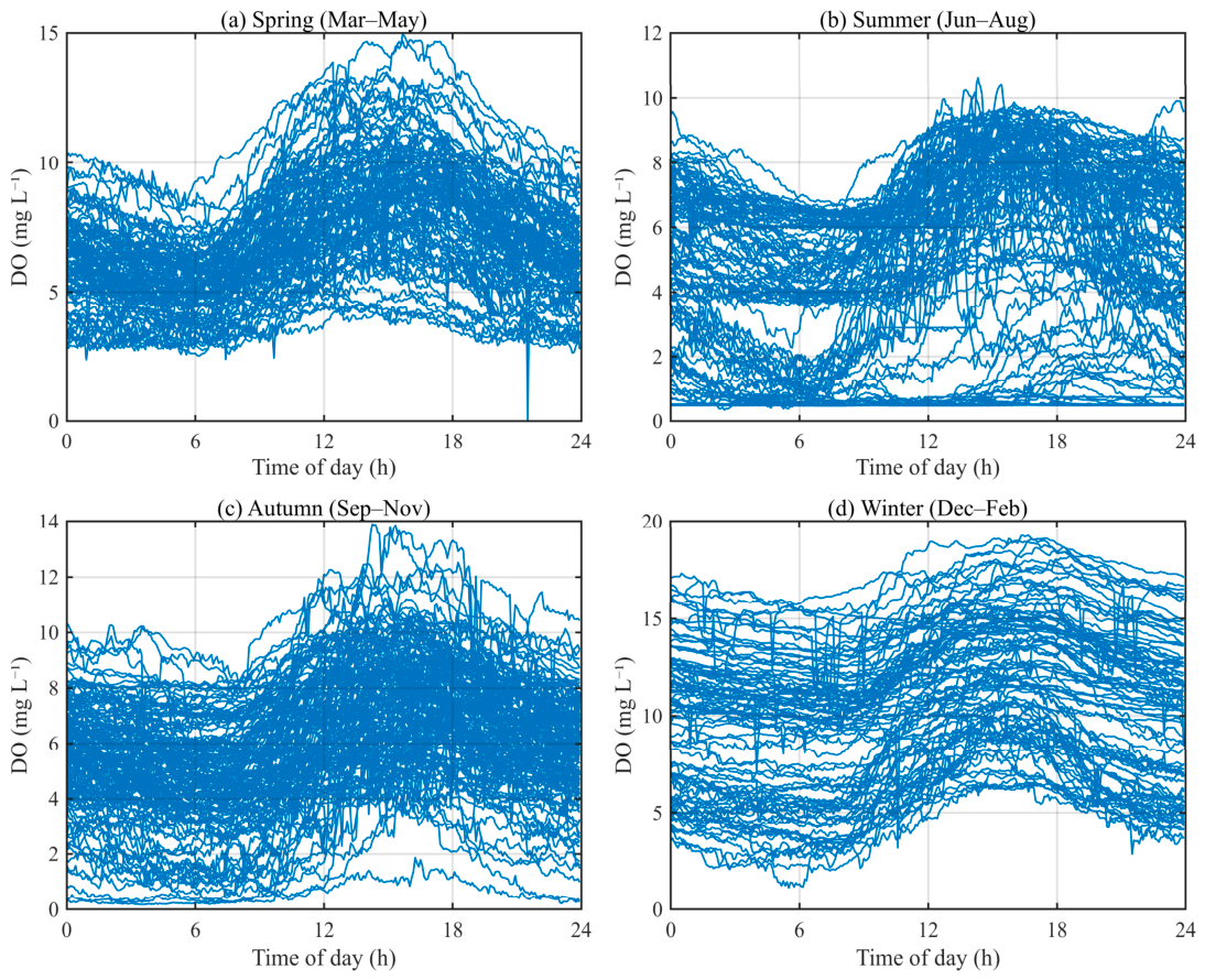
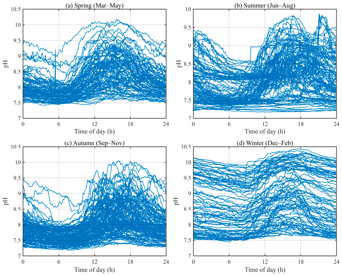
High-frequency monitoring revealed distinct diel and seasonal differences among the four physicochemical variables (Figure 2). DO and pH exhibited the most pronounced diel oscillations, with generally lower values during nighttime and early morning and repeated increases during daytime (Figure 2a,c). Water temperature showed smoother within-day variation but a wide seasonal range, reflecting strong seasonal thermal differences (Figure 2b). In contrast, EC showed no consistent diel pattern and remained mostly within a relatively narrow range, although occasional abrupt fluctuations were observed (Figure 2d). These abrupt EC excursions may have been associated with short-term external or operational influences, such as rainfall dilution, shallow-water mixing, local hydrodynamic disturbance, sensor noise, or maintenance-related effects. However, because EC showed weak diel regularity and limited coupling with DO and pH, it was not used as a core indicator for subsequent oxygen-stress threshold analysis. Overall, DO and pH were the most responsive variables at the diel scale; whereas, temperature mainly reflected seasonal background variation and EC showed comparatively weak short-term regularity.

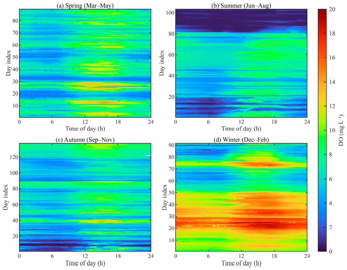
The seasonal DO heatmaps showed pronounced seasonal and diel variation in oxygen conditions (Figure 3). In spring, DO concentrations were generally moderate, with repeated daytime increases and relatively limited low-DO zones. Summer exhibited the most extensive low-DO conditions, particularly during the early and late parts of the season, when low DO persisted over much of the diel cycle. Autumn also showed low-DO zones, especially during the early seasonal period, but these conditions became less persistent later in the season. In contrast, winter was characterized by generally higher DO concentrations, with broad high-DO bands occurring mainly during daytime and afternoon periods. Overall, low-oxygen conditions occurred repeatedly rather than as isolated observations, and were most pronounced in summer, followed by early autumn.

The 3D surface plots showed a clear positive coupling between DO and pH across representative seasonal periods (Figure 4). Higher DO concentrations generally corresponded to higher pH values, especially during daytime; whereas, lower DO levels were associated with reduced pH. This pattern indicates that DO and pH varied synchronously at the diel scale, while temperature mainly reflected seasonal background conditions.

3.2. Selection of Key Ecological Indicators

The diel dynamics and seasonal variability of DO and pH are shown in Figure 5 and Figure 6, while the corresponding seasonal patterns of water temperature and EC are provided in Supplementary Figures S2 and S3. DO and pH exhibited pronounced and synchronized diel oscillations across seasons, with daytime increases and nighttime declines. The magnitude of diel fluctuations was greater during warm seasons, particularly in summer, when extended nighttime low-DO conditions were observed. In contrast, temperature mainly reflected seasonal differences and showed relatively smooth within-day variation; whereas, EC exhibited no obvious diel pattern and showed the smallest within-day fluctuation during the monitoring period.

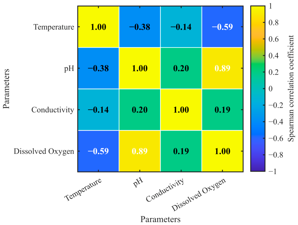
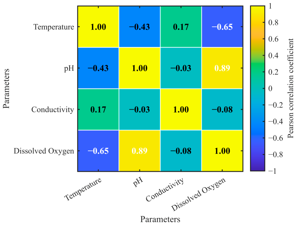
Correlation analysis further confirmed the close coupling between DO and pH. Spearman correlation showed a strong positive relationship between DO and pH (ρ = 0.89), which was consistent with the Pearson correlation result (r = 0.89). The consistency between Spearman and Pearson correlations indicated that the DO–pH coupling was robust across different correlation assumptions, reflecting both a strong monotonic association and a strong linear relationship. Temperature was negatively correlated with both DO (ρ = −0.59; r = −0.65) and pH (ρ = −0.38; r = −0.43), indicating that warmer conditions were generally associated with lower oxygen concentrations and lower pH. In contrast, electrical conductivity showed relatively weak correlations with the other variables, and the correlation direction was not fully consistent between Spearman and Pearson analyses, suggesting that EC mainly reflected hydrochemical background conditions and possible short-term disturbance signals rather than diel metabolic variability.

Overall, the correlation matrices showed that DO had the closest association with pH among the monitored variables, while both variables were negatively associated with temperature (Figure 7 and Figure 8). Because DO directly represents oxygen availability and low-oxygen stress, it was selected for subsequent threshold detection and oxygen-stress accumulation analysis.

3.3. Threshold Dynamics and Progressive Deterioration of Oxygen Recovery

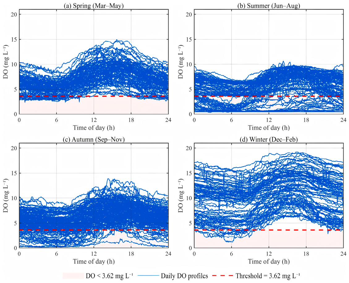
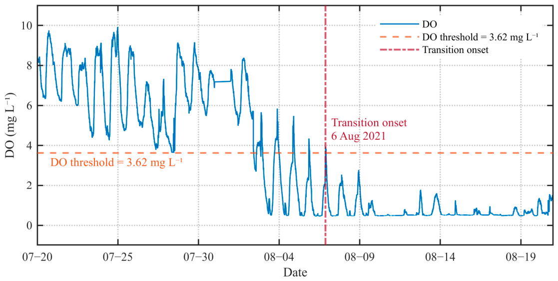
Since DO was identified as the most informative parameter for describing short-term ecosystem instability and oxygen-related stress based on the indicator-screening results (Section 3.2), it was selected for threshold detection and for analyzing the transition toward persistent low-oxygen conditions. The threshold–log-likelihood analysis identified an optimal DO threshold of 3.62 mg L⁻¹ (Figure 9a). The sensitivity analysis showed that alternative definitions of the hypoxia-related oxygen-stress state produced similar threshold estimates, ranging from 3.51 to 3.77 mg L⁻¹ (Table S3). Thresholds based on low-oxygen duration criteria of >2 and >4 h d⁻¹ were 3.63 and 3.58 mg L⁻¹, respectively; whereas, OSEI-based criteria using the 75th and 80th percentiles yielded thresholds of 3.64 and 3.51 mg L⁻¹, respectively. These results indicate that the identified threshold was not determined by a single operational definition of oxygen stress. This threshold corresponded to the maximum log-likelihood and therefore represented the most pronounced DO-based transition point toward persistent low-oxygen conditions. Piecewise logistic regression further revealed a nonlinear relationship between daily minimum DO and the probability of persistent hypoxia-related oxygen-stress states (Figure 9b). Seasonal diel DO variations further showed that DO generally remained above 3.62 mg L⁻¹ during spring and winter; whereas, below-threshold conditions occurred more frequently and persisted for longer durations during summer and autumn (Figure 10). This seasonal pattern coincided with periods of increased oxygen-stress exposure and greater DO instability. In August 2021, diel DO fluctuations declined rapidly after 4 August, accompanied by reduced diel amplitude, intensified nocturnal oxygen depletion, and increasingly frequent below-threshold episodes. Although several low-DO events occurred before the transition toward persistent low-oxygen conditions, the system initially retained the capacity to recover above the threshold during daytime. As oxygen-stress events accumulated, daytime recovery progressively weakened, and the duration of low-oxygen exposure increased. By 6 August, DO peaks had declined to levels close to the identified threshold, indicating that daytime recovery was no longer sufficient to offset nocturnal oxygen losses. Consequently, the system entered a persistent low-oxygen state after 6 August (Figure 11).

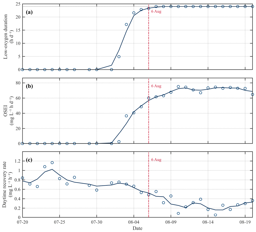
Quantitative indicators further revealed substantial changes in oxygen-stress exposure and recovery dynamics during the transition period (Figure 12). Low-oxygen duration remained close to zero before 2 August but increased rapidly thereafter, reaching more than 20 h d⁻¹ by 4 August and approaching continuous exposure (24 h d⁻¹) after 6 August (Figure 12a). Concurrently, the oxygen-stress exposure index (OSEI) increased sharply from 2.36 mg L⁻¹ h d⁻¹ on 2 August to more than 60 mg L⁻¹ h d⁻¹ after 6 August, indicating a rapid increase in cumulative oxygen deficit (Figure 12b). In contrast, daytime recovery rate declined progressively throughout the transition period, decreasing from approximately 0.75 mg L⁻¹ h⁻¹ in early August to below 0.50 mg L⁻¹ h⁻¹ after 6 August (Figure 12c). These temporal changes marked the transition from transient low-oxygen episodes to persistent low-oxygen conditions after 6 August.

3.4. PCA of High-Frequency Physicochemical Variables

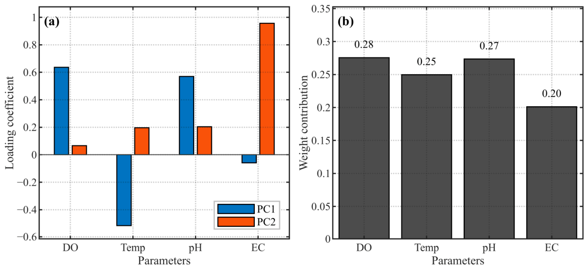
After Z-score standardization, PCA on DO, temperature, pH, and EC showed that PC1 and PC2 explained 83.7% of total variance (PC1: 57.9%; PC2: 25.8%). Loadings indicated PC1 was dominated by positive loadings of DO and pH and a negative loading of temperature (Figure 13a). PC2 was dominated by EC (Figure 13a). Composite weights based on absolute loadings and variance contributions yielded DO = 0.28, pH = 0.27, temperature = 0.25, and EC = 0.20 (Figure 13b).

3.5. PLS-SEM Path Analysis

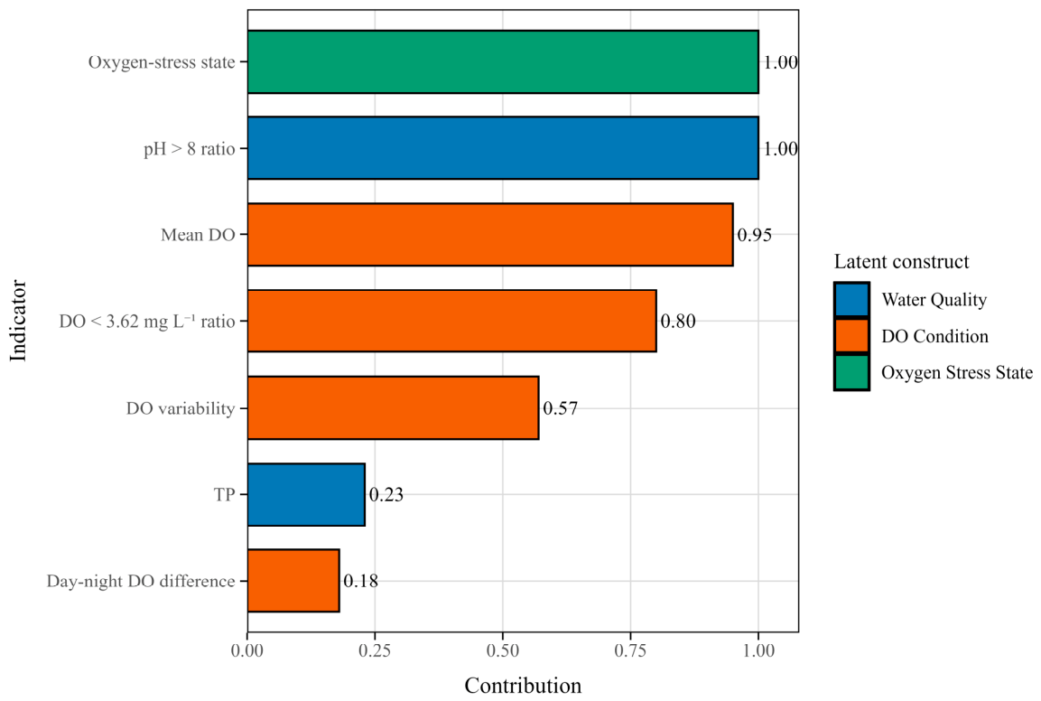
The indicator-importance results indicated that the pH > 8 ratio was the dominant indicator of water quality (Figure 14). Mean DO and the DO < 3.62 mg L⁻¹ ratio contributed most strongly to DO Condition; whereas, day–night DO difference showed the weakest contribution. Oxygen-stress state was specified as a single-indicator construct with a fixed contribution of 1.00.

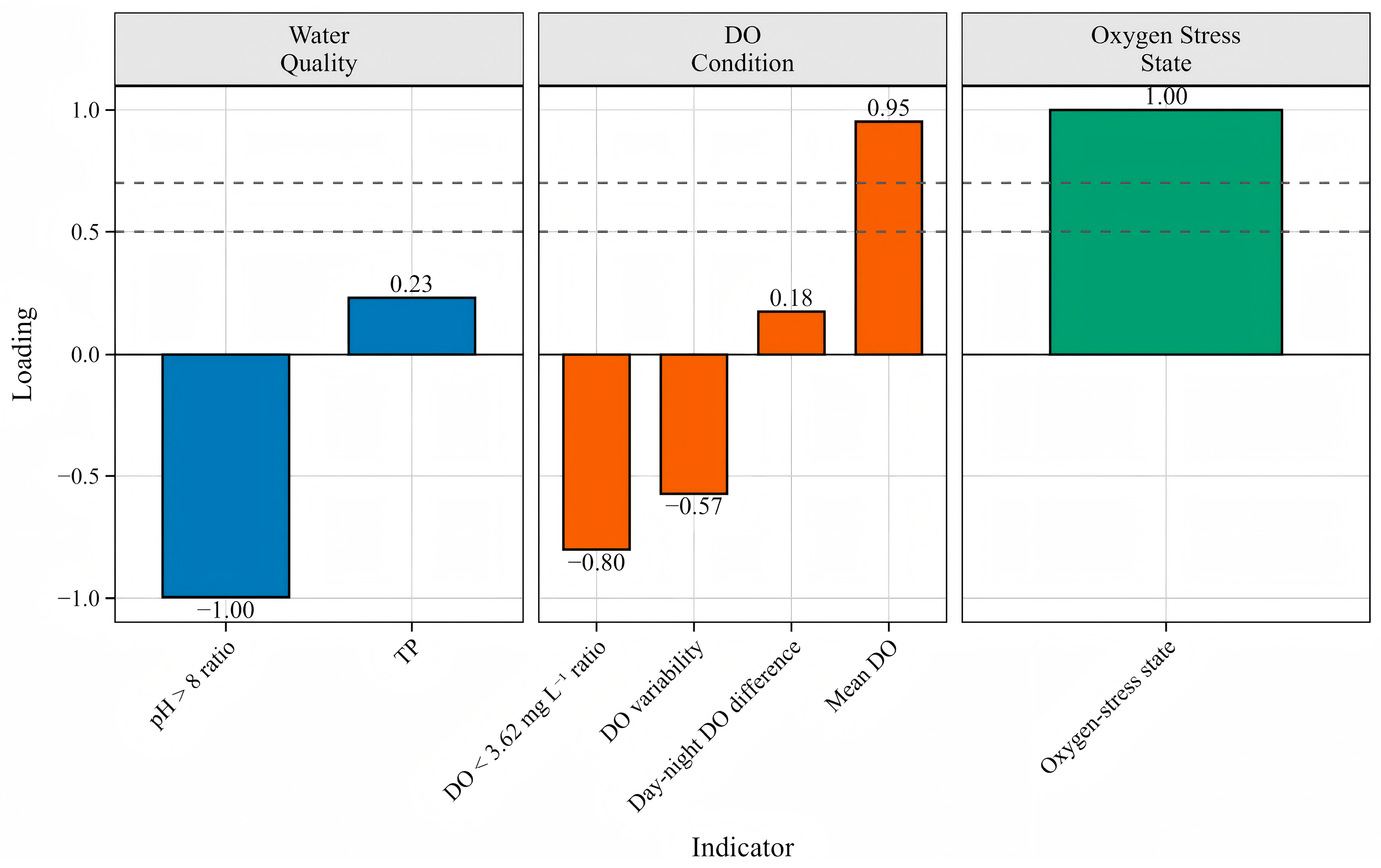
The indicator-loading results (Figure 15) showed that the water quality construct was mainly characterized by the pH > 8 ratio, with a strong negative loading of −1.00; whereas, TP showed a weak loading of 0.23. The DO Condition construct was primarily represented by Mean DO and the DO < 3.62 mg L⁻¹ ratio, with loadings of 0.95 and −0.80, respectively. DO variability showed a moderate loading of −0.57, while day–night DO difference showed a comparatively weak loading of 0.18. Oxygen-stress state was specified as a single-indicator construct and therefore had a fixed loading of 1.00.

Reliability and convergent-validity diagnostics were further calculated for the exploratory PLS-SEM measurement model (

Table 2. Reliability and convergent-validity diagnostics of the exploratory PLS-SEM measurement model.

Construct	Indicators	Cronbach’s α	CR	AVE	Interpretation
Water Quality	TP; pH > 8 ratio	0.48	0.61	0.53	AVE was acceptable, but internal consistency was relatively weak
DO Condition	Mean DO; DO < 3.62 mg L−1 ratio; DO variability; day–night DO difference	0.67	0.75	0.48	CR was acceptable; whereas, AVE was slightly below 0.50
Oxygen-Stress State	Oxygen-stress state	N/A	N/A	N/A	Single-indicator construct

Note: CR, composite reliability; AVE, average variance extracted. Cronbach’s α was calculated using direction-adjusted standardized indicators, and CR and AVE were calculated using direction-adjusted standardized outer loadings. Oxygen-stress state was specified as a single-indicator construct; therefore, Cronbach’s α, CR, and AVE were not applicable. Given the limited monthly sample size, these diagnostics were interpreted as exploratory rather than confirmatory evidence.

). For water quality, Cronbach’s α, CR, and AVE were 0.48, 0.61, and 0.53, respectively. These results indicated acceptable convergent validity but relatively weak internal consistency, mainly because TP showed a weak loading compared with the pH > 8 ratio. For DO Condition, Cronbach’s α, CR, and AVE were 0.67, 0.75, and 0.48, respectively, indicating acceptable composite reliability but slightly weak convergent validity. The slightly low AVE was mainly associated with the weak loading of day–night DO difference. Oxygen-stress state was specified as a single-indicator construct, so Cronbach’s α, CR, and AVE were not applicable.

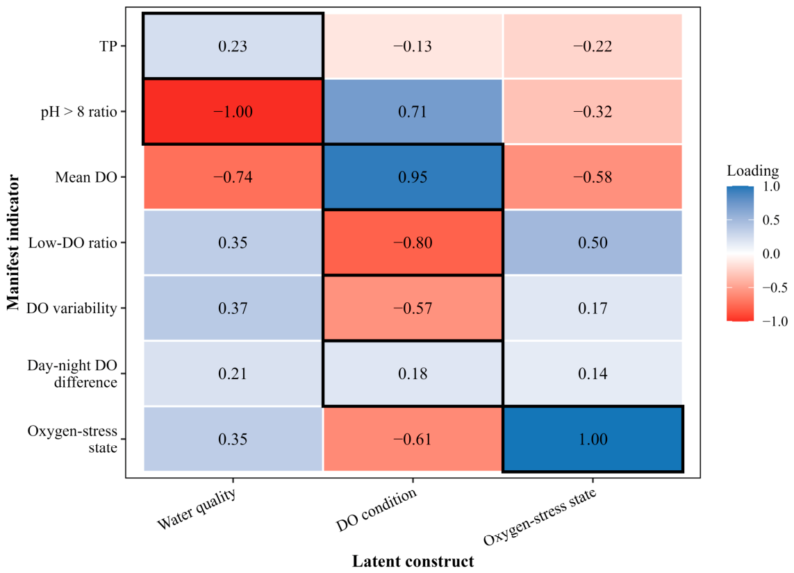
The cross-loading matrix generally supported the measurement structure of the PLS-SEM model according to commonly used PLS-SEM criteria [32,36], as most manifest indicators showed their highest absolute loadings on their predefined latent constructs (Figure 16).

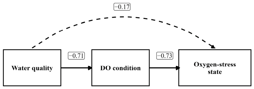
The PLS-SEM structural path diagram showed that water quality was negatively associated with DO Condition, with a standardized path coefficient of −0.71 (Figure 17). DO Condition was further negatively associated with the oxygen-stress state, with a path coefficient of −0.73. In contrast, the direct path from water quality to the oxygen-stress state was relatively weak (−0.17), indicating that the influence of water-quality variation on oxygen-stress development was mainly mediated through DO Condition. The complete PLS-SEM structural path diagram is provided in Supplementary Figure S1.

Taken together, these results suggest that the observed monthly patterns were consistent with a water quality → DO Condition → Oxygen-stress state pathway, in which the effect of water-quality variation on oxygen-stress development was mainly transmitted through changes in DO Condition. However, because the PLS-SEM analysis was exploratory and based on monthly scale observations, this pathway should be interpreted as an associative mechanism rather than evidence of strict causality.

4. Discussion

4.1. Ecological Roles of Four High-Frequency Environmental Parameters

The four monitored high-frequency physicochemical variables exhibited distinct ecological functions and together provided complementary information for describing short-term ecosystem dynamics. Unlike conventional water-quality indicators that are often measured at low temporal frequency, dissolved oxygen (DO), pH, temperature, and electrical conductivity (EC) can be continuously monitored and respond rapidly to environmental change. Their high-frequency observations therefore provide direct insight into ecosystem processes operating at diel timescales [2,6,22].

Among the four parameters, DO showed the strongest ecological responsiveness. Seasonal diel curves revealed pronounced fluctuations between daytime oxygen production and nighttime oxygen depletion, while correlation analysis and PCA further identified DO as the most influential variable. Because DO integrates photosynthesis, respiration, organic matter decomposition, and atmospheric exchange, it reflects ecosystem metabolic balance and oxygen-related system conditions [9,13,14]. The threshold analysis further indicated that changes in DO were closely associated with the development of persistent low-oxygen conditions, thereby supporting the role of DO as a key indicator of short-term oxygen instability.

The pH exhibited diel dynamics closely coupled with DO and showed the strongest positive correlation among all parameter pairs. This relationship reflects the shared influence of photosynthesis and respiration on oxygen and carbon cycling within the lake ecosystem [37]. In contrast, temperature primarily acted as a metabolic driver, regulating biological activity, oxygen demand, and oxygen solubility [38,39,40]. EC exhibited comparatively weak diel variability and weaker coupling with other variables, suggesting that it mainly reflected hydrochemical background conditions and potential short-term external disturbance signals rather than direct metabolic variability [41,42]. Therefore, the occasional EC spikes observed in the high-frequency record were interpreted cautiously as possible short-term disturbance or measurement-related signals rather than as evidence of persistent metabolic change.

Collectively, the four parameters represent complementary dimensions of ecosystem functioning, with DO serving as the core response indicator of oxygen instability, pH indicating metabolic coupling, temperature regulating metabolic intensity, and EC providing a background hydrochemical reference. However, the results consistently indicated that DO occupied a central position linking environmental variability to the development of persistent hypoxia-related oxygen-stress conditions. This finding provides process-based support for interpreting the threshold analysis and highlights the value of high-frequency DO monitoring for early detection of oxygen instability in eutrophic shallow lakes.

4.2. Threshold Dynamics and Daily Accumulation of Oxygen Stress

Threshold analysis identified a site-specific dissolved oxygen threshold of 3.62 mg L⁻¹, below which the probability of persistent hypoxia-related oxygen-stress states increased markedly. The ecological relevance of this threshold is supported by previous studies. A global synthesis of 872 experiments involving 206 species demonstrated that many aquatic organisms exhibit lethal or sublethal responses when dissolved oxygen concentrations decline to 2–5 mg L⁻¹ [43]. Importantly, high-frequency observations showed that threshold exceedance was not instantaneous. Instead, it was preceded by a sequence of recurrent daily metabolic interruptions: intensified nocturnal oxygen depletion, reduced diel amplitude, and incomplete daytime oxygen recovery. These patterns developed progressively over multiple days rather than emerging abruptly when DO fell below the threshold.

Ecologically, each nocturnal hypoxia episode can be interpreted as a small-scale interruption of normal metabolic functioning. While any single interruption may appear transient, repeated occurrences can increase physiological stress, reduce recovery efficiency, and weaken ecosystem resilience. Similar resilience-based assessment frameworks have emphasized that ecosystem vulnerability is often determined not only by disturbance intensity but also by the capacity for recovery following repeated stress events [44,45]. As these interruptions accumulate, the system becomes increasingly vulnerable to threshold transitions and subsequent ecological deterioration [44,46,47,48]. This daily accumulation perspective also reframes management targets: preventing large-scale transitions requires reducing the mechanism that permits repeated daily oxygen-stress buildup, rather than focusing only on static nutrient or biomass snapshots.

The transition-period analysis provides quantitative support for this accumulation process. Following the initial threshold exceedances, low-oxygen duration increased rapidly from near-zero to near-continuous exposure, while oxygen-stress exposure increased more than 20-fold within several days. At the same time, daytime recovery rate declined progressively, indicating a reduced capacity for daytime oxygen replenishment. These changes occurred concurrently with the establishment of persistent low-oxygen conditions after 6 August. Rather than reflecting a single threshold-crossing event, the transition from transient low-oxygen episodes to persistent low-oxygen conditions was preceded by increasing oxygen-stress exposure and progressively weakened daytime recovery. Similar patterns have been reported in ecosystems approaching ecological deterioration, where repeated stress events and reduced recovery capacity contribute to declining resilience and increased vulnerability to regime shifts [49].

In this sense, DO-based prediction gains reliability not only from statistical threshold detection, but also from the concordance between threshold timing and the observed trajectory of oxygen-stress accumulation and recovery deterioration. The progressive increase in low-oxygen duration and oxygen-stress exposure, together with declining daytime recovery rates, provides a process-based interpretation of oxygen instability before the transition toward persistent low-oxygen conditions. Such temporal shifts are broadly consistent with previous observations that increasing instability and altered ecosystem dynamics may precede ecological deterioration [45]. The sensitivity analysis further supported the relative stability of the identified DO threshold under alternative oxygen-stress definitions (Table S3). Nevertheless, because all threshold estimates were derived from site-specific high-frequency DO dynamics and operational stress-state definitions, the threshold should be interpreted as an early-warning threshold for persistent hypoxia-related oxygen stress rather than as a universal ecological threshold.

Although the threshold and early-warning indicators were derived from high-frequency DO dynamics, meteorological and hydrological forcing may have modulated the observed diel oxygen patterns. Wind can affect shallow-lake mixing and alter the balance between surface reaeration and oxygen redistribution and localized oxygen depletion. Rainfall and urban runoff may introduce short-term dilution, nutrient inputs, organic matter, and suspended particles, thereby changing light availability, primary production, respiration, and oxygen demand. Water-level fluctuations may further influence water exchange, residence time, and sediment–water interactions. In addition, high temperature can reduce oxygen solubility while enhancing biological respiration and organic-matter decomposition, thereby increasing the likelihood of nighttime oxygen depletion [28,38,39,40]. These external drivers were not explicitly quantified in the present study; therefore, the observed oxygen-stress accumulation should be interpreted as the combined result of internal metabolic processes and potential short-term external forcing. Future studies should integrate high-frequency DO monitoring with meteorological, hydrological, and runoff observations to better distinguish internally driven metabolic instability from externally forced oxygen fluctuations.

4.3. Ecological Mechanisms Underlying the Central Role of Dissolved Oxygen

PCA indicated that DO and pH form the dominant environmental gradient, while temperature and EC contribute as additional axes with different functional roles. The dominance of DO and pH suggests that short-term ecosystem variability in this eutrophic shallow lake was primarily governed by metabolic processes. DO reflects the metabolic balance between photosynthesis and respiration and therefore captures the ecosystem’s recovery capacity and trajectory of instability. pH responds sensitively to photosynthetic carbon uptake and serves as an indicator of biological production and algal activity [37]. Temperature primarily modulates metabolic intensity and thus the propensity for oxygen instability [38,39]; whereas, EC largely represents background hydrochemical conditions and external influences with weaker short-term coupling to metabolic dynamics [41,42].

The exploratory PLS-SEM analysis further suggested that changes in DO conditions may serve as an important process-based indicator linking water-quality pressure with persistent hypoxia-related oxygen-stress states. The strong path coefficient from Water_Quality to DO_Condition and the dominant direct path coefficient from DO_Condition to oxygen-stress state indicate that oxygen dynamics may play a potential mediating role between environmental variability and persistent hypoxia-related oxygen-stress states. This exploratory pathway is consistent with the PCA results, which identified a dominant environmental gradient characterized by coupled variation in DO- and pH-related parameters.

The central role of DO is ecologically reasonable because dissolved oxygen integrates multiple fast-responding ecosystem processes, including primary production, community respiration, and oxygen consumption associated with the decomposition of organic matter [9,14,37,39]. In eutrophic shallow lakes, enhanced primary productivity can simultaneously elevate pH and increase daytime oxygen concentrations; whereas, nighttime respiration may result in substantial oxygen depletion before sunrise. Such coupled fluctuations in pH and DO are widely recognized as characteristic features of metabolically active shallow-lake ecosystems [50].

The strong contributions of DO_mean and DO_below3.62_ratio in the PLS-SEM model further suggest that overall oxygen status and below-threshold oxygen exposure may represent key process-based indicators through which water-quality pressure is reflected in persistent hypoxia-related oxygen-stress states. Previous studies have shown that prolonged hypoxia can affect fish, zooplankton, benthic organisms, and microbial communities, often reducing ecosystem resilience and increasing vulnerability to ecological disturbance [51,52,53,54]. These observations are consistent with the threshold analysis presented in this study, which identified a site-specific DO threshold of approximately 3.62 mgL⁻¹ associated with increased likelihood of persistent hypoxia-related oxygen-stress states.

Because DO integrates and responds rapidly to these ecosystem processes, changes in DO behavior can emerge earlier than substantial changes become detectable in many conventional low-frequency indicators. The cross-loading patterns observed in the measurement model further suggest that water-quality variation and oxygen dynamics were not fully independent. Similar coupling has been reported in eutrophic lakes, where nutrient enrichment alters ecosystem metabolism, amplifies diel oxygen fluctuations, and increases the occurrence of low-oxygen events [40,55]. Phosphorus plays a particularly important role in regulating primary productivity and metabolic responses in aquatic ecosystems, thereby influencing oxygen dynamics and ecosystem stability [56]. Consequently, ecological deterioration may develop through the cumulative effects of recurring oxygen stress rather than through abrupt changes in conventional water-quality variables.

This exploratory pathway is consistent with the daily accumulation interpretation: water-quality pressure may be reflected in altered DO dynamics, and repeated DO deterioration may increase the likelihood of transition toward persistent low-oxygen conditions. Rather than representing a single disturbance event, persistent hypoxia-related oxygen stress may develop through the accumulation of small metabolic disruptions during daily ecosystem processes.

Overall, the combined results from PCA and exploratory PLS-SEM suggest that DO dynamics provide a process-based pathway through which water-quality pressure can be reflected in threshold behavior, pre-transition patterns, and persistent hypoxia-related oxygen-stress states. This pathway is broadly consistent with the nutrient enrichment–oxygen depletion–ecological deterioration sequence reported in eutrophic lake ecosystems [18,46,47,48]. Together, these findings highlight the potential of high-frequency DO monitoring to support early warning of hypoxia-related oxygen stress and improve process-based ecosystem assessment in shallow eutrophic lakes.

4.4. Limitations and Future Validation

Several limitations should be acknowledged when interpreting the findings of this study. First, the analysis was based on high-frequency monitoring from a single shallow eutrophic lake and a single monitoring site. The sensors were deployed at a fixed depth of approximately 0.5 m below the water surface; therefore, the observed DO dynamics mainly represented near-surface conditions at the monitoring site rather than vertically integrated whole-lake oxygen conditions. Although this design allowed detailed characterization of temporal oxygen dynamics at a fixed monitoring depth, it could not fully capture horizontal spatial heterogeneity or vertical differences between surface and near-bottom waters. Therefore, the identified DO threshold should be interpreted as site-specific and depth-specific, and should not be directly generalized to other lakes, monitoring depths, or whole-lake conditions without further validation.

Second, the binary oxygen-stress state used in this study was derived from high-frequency DO dynamics rather than from independent biological-response observations. The identified threshold therefore represents a process-based early-warning threshold for persistent hypoxia-related oxygen stress, not a threshold of confirmed biological damage. Future studies should integrate high-frequency DO monitoring with chlorophyll-a, water transparency, algal community composition, fish responses, zooplankton, and benthic-community observations to evaluate how oxygen-stress accumulation translates into biological and ecological consequences.

Third, TP was used as a monthly nutrient-pressure indicator in the exploratory PLS-SEM analysis, but other nutrient and biological variables, including total nitrogen, N:P ratio, chlorophyll-a, and algal biomass, were not available at comparable temporal resolution. This limitation restricts the ability to fully resolve nutrient limitation, algal dynamics, and their coupling with DO variability. Future work should combine high-frequency sensor observations with more complete nutrient and biological monitoring to strengthen the interpretation of nutrient–oxygen–stress pathways.

Finally, potential external drivers, including rainfall, urban runoff, wind-driven mixing, water-level changes, and episodic hydrological disturbances, were not explicitly quantified in the present analysis. These factors may influence diel oxygen dynamics and the timing of low-oxygen events. Multi-site, multi-depth, and multi-lake monitoring, combined with meteorological and hydrological observations, will be necessary to test the transferability of the proposed threshold and early-warning indicators.

5. Conclusions

The results of this study suggest that assessment of eutrophic shallow lakes should place greater emphasis on high-frequency monitoring of DO dynamics and the cumulative effects of repeated daily oxygen stress. Unlike conventional assessments that rely primarily on infrequent measurements of nutrient concentrations or algal biomass, high-frequency observations of DO, pH, temperature, and EC provide process-level information on short-term metabolic variability and oxygen instability.

By integrating diel fluctuation analysis, threshold detection, PCA, and exploratory PLS-SEM, this study showed that high-frequency physicochemical variables can be used to identify site-specific statistical hypoxia thresholds, quantify oxygen instability, and evaluate how DO dynamics reflect environmental variability and persistent hypoxia-related oxygen-stress states. The transition from transient low-oxygen episodes to persistent low-oxygen conditions was accompanied by progressive declines in daily minimum DO and daytime recovery capacity, together with increasing low-oxygen duration, indicating that persistent hypoxia emerged through the accumulation of repeated oxygen-stress events rather than from a single threshold-crossing event.

These findings demonstrate the potential of high-frequency DO monitoring to support early warning of hypoxia-related oxygen stress in shallow eutrophic lakes. The identified threshold of 3.62 mg L⁻¹ should be interpreted as a site-specific, process-based early-warning threshold for persistent hypoxia-related oxygen stress rather than as a universal ecological threshold or a threshold of confirmed biological damage.

References

1. Anastasopoulos, P.; Akratos, C.S. A Review on Water Quality Indices. Hydroecol. Eng. 2025, 2, 10003. [Google Scholar] [CrossRef]
2. Rozemeijer, J.; Jordan, P.; Hooijboer, A.; Kronvang, B.; Glendell, M.; Hensley, R.; Rinke, K.; Stutter, M.; Bieroza, M.; Turner, R.; et al. Best Practice in High-Frequency Water Quality Monitoring for Improved Management and Assessment; a Novel Decision Workflow. Environ. Monit. Assess. 2025, 197, 353. [Google Scholar] [CrossRef] [PubMed]
3. Carpenter, S.R.; Cole, J.J.; Pace, M.L.; Batt, R.; Brock, W.A.; Cline, T.; Coloso, J.; Hodgson, J.R.; Kitchell, J.F.; Seekell, D.A.; et al. Early Warnings of Regime Shifts: A Whole-Ecosystem Experiment. Science 2011, 332, 1079–1082. [Google Scholar] [CrossRef] [PubMed]
4. Rode, M.; Wade, A.J.; Cohen, M.J.; Hensley, R.T.; Bowes, M.J.; Kirchner, J.W.; Arhonditsis, G.B.; Jordan, P.; Kronvang, B.; Halliday, S.J.; et al. Sensors in the Stream: The High-Frequency Wave of the Present. Environ. Sci. Technol. 2016, 50, 10297–10307. [Google Scholar] [CrossRef] [PubMed]
5. Gsell, A.S.; Teurlincx, S.; Adrian, R.; Janssen, A.B.G. Timing Matters: Sampling Frequency for Early-Warning Indicators across Food Web Components in a Virtual Lake. Ecol. Indic. 2023, 153, 110424. [Google Scholar] [CrossRef]
6. Wilhelm, S.; Adrian, R. Impact of Summer Warming on the Thermal Characteristics of a Polymictic Lake and Consequences for Oxygen, Nutrients and Phytoplankton. Freshw. Biol. 2008, 53, 226–237. [Google Scholar] [CrossRef]
7. Coloso, J.J.; Cole, J.J.; Pace, M.L. Difficulty in Discerning Drivers of Lake Ecosystem Metabolism with High-Frequency Data. Ecosystems 2011, 14, 935–948. [Google Scholar] [CrossRef]
8. Obertegger, U.; Obrador, B.; Flaim, G. Dissolved Oxygen Dynamics under Ice: Three Winters of High-Frequency Data from Lake Tovel, Italy. Water Resour. Res. 2017, 53, 7234–7246. [Google Scholar] [CrossRef]
9. Staehr, P.A.; Bade, D.; Van De Bogert, M.C.; Koch, G.R.; Williamson, C.; Hanson, P.; Cole, J.J.; Kratz, T. Lake Metabolism and the Diel Oxygen Technique: State of the Science. Limnol. Oceanogr. Methods 2010, 8, 628–644. [Google Scholar] [CrossRef]
10. Istvánovics, V.; Honti, M. Coupled Simulation of High-frequency Dynamics of Dissolved Oxygen and Chlorophyll Widens the Scope of Lake Metabolism Studies. Limnol. Oceanogr. 2018, 63, 72–90. [Google Scholar] [CrossRef]
11. Rodriguez-Perez, J.; Leigh, C.; Liquet, B.; Kermorvant, C.; Peterson, E.; Sous, D.; Mengersen, K. Detecting Technical Anomalies in High-Frequency Water-Quality Data Using Artificial Neural Networks. Environ. Sci. Technol. 2020, 54, 13719–13730. [Google Scholar] [CrossRef] [PubMed]
12. O’Brien, D.A.; Deb, S.; Gal, G.; Thackeray, S.J.; Dutta, P.S.; Matsuzaki, S.S.; May, L.; Clements, C.F. Early Warning Signals Have Limited Applicability to Empirical Lake Data. Nat. Commun. 2023, 14, 7942. [Google Scholar] [CrossRef] [PubMed]
13. Odum, H.T. Primary Production in Flowing Waters1. Limnol. Oceanogr. 1956, 1, 102–117. [Google Scholar] [CrossRef]
14. Solomon, C.T.; Bruesewitz, D.A.; Richardson, D.C.; Rose, K.C.; Van De Bogert, M.C.; Hanson, P.C.; Kratz, T.K.; Larget, B.; Adrian, R.; Babin, B.L.; et al. Ecosystem Respiration: Drivers of Daily Variability and Background Respiration in Lakes around the Globe. Limnol. Oceanogr. 2013, 58, 849–866. [Google Scholar] [CrossRef]
15. Altieri, A.H.; Gedan, K.B. Climate Change and Dead Zones. Glob. Change Biol. 2015, 21, 1395–1406. [Google Scholar] [CrossRef] [PubMed]
16. Dugener, N.M.; Weinke, A.D.; Stone, I.P.; Biddanda, B.A. Recurringly Hypoxic: Bottom Water Oxygen Depletion Is Linked to Temperature and Precipitation in a Great Lakes Estuary. Hydrobiology 2023, 2, 410–430. [Google Scholar] [CrossRef]
17. Stelzer, J.A.A.; Mesman, J.P.; Adrian, R.; Ibelings, B.W. Early Warning Signals of Regime Shifts for Aquatic Systems: Can Experiments Help to Bridge the Gap between Theory and Real-World Application? Ecol. Complex. 2021, 47, 100944. [Google Scholar] [CrossRef]
18. Jeppesen, E.; Søndergaard, M.; Meerhoff, M.; Lauridsen, T.L.; Jensen, J.P. Shallow Lake Restoration by Nutrient Loading Reduction—Some Recent Findings and Challenges Ahead. Hydrobiologia 2007, 584, 239–252. [Google Scholar] [CrossRef]
19. Murphy, J.; Riley, J.P. A Modified Single Solution Method for the Determination of Phosphate in Natural Waters. Anal. Chim. Acta 1962, 27, 31–36. [Google Scholar] [CrossRef]
20. APHA; AWWA; WEF. Standard Methods for the Examination of Water and Wastewater, 23rd ed.; American Public Health Association: Washington, DC, USA, 2017. [Google Scholar]
21. Peeters, F.; Atamanchuk, D.; Tengberg, A.; Encinas-Fernández, J.; Hofmann, H. Lake Metabolism: Comparison of Lake Metabolic Rates Estimated from a Diel CO2- and the Common Diel O2-Technique. PLoS ONE 2016, 11, e0168393. [Google Scholar] [CrossRef] [PubMed]
22. Winslow, L.A.; Zwart, J.A.; Batt, R.D.; Dugan, H.A.; Woolway, R.I.; Corman, J.R.; Hanson, P.C.; Read, J.S. LakeMetabolizer: An R Package for Estimating Lake Metabolism from Free-Water Oxygen Using Diverse Statistical Models. Inland Waters 2016, 6, 622–636. [Google Scholar] [CrossRef]
23. Rose, K.C.; Weathers, K.C.; Hetherington, A.L.; Hamilton, D.P. Insights from the Global Lake Ecological Observatory Network (GLEON). Inland Waters 2016, 6, 476–482. [Google Scholar] [CrossRef]
24. Giling, D.P.; Staehr, P.A.; Grossart, H.P.; Andersen, M.R.; Boehrer, B.; Escot, C.; Evrendilek, F.; Gómez-Gener, L.; Honti, M.; Jones, I.D.; et al. Delving Deeper: Metabolic Processes in the Metalimnion of Stratified Lakes. Limnol. Oceanogr. 2017, 62, 1288–1306. [Google Scholar] [CrossRef]
25. Stefanidis, K.; Dimitriou, E. Differentiation in Aquatic Metabolism between Littoral Habitats with Floating-Leaved and Submerged Macrophyte Growth Forms in a Shallow Eutrophic Lake. Water 2019, 11, 287. [Google Scholar] [CrossRef]
26. Hu, Z.; Xiao, Q.; Yang, J.; Xiao, W.; Wang, W.; Liu, S.; Lee, X. Temporal Dynamics and Drivers of Ecosystem Metabolism in a Large Subtropical Shallow Lake (Lake Taihu). Int. J. Environ. Res. Public Health 2015, 12, 3691–3706. [Google Scholar] [CrossRef] [PubMed]
27. Martinsen, K.T.; Zak, N.B.; Baastrup-Spohr, L.; Kragh, T.; Sand-Jensen, K. Ecosystem Metabolism and Gradients of Temperature, Oxygen and Dissolved Inorganic Carbon in the Littoral Zone of a Macrophyte-Dominated Lake. JGR Biogeosci. 2022, 127, e2022JG007193. [Google Scholar] [CrossRef]
28. Kraemer, B.M.; Pilla, R.M.; Woolway, R.I.; Anneville, O.; Ban, S.; Colom-Montero, W.; Devlin, S.P.; Dokulil, M.T.; Gaiser, E.E.; Hambright, K.D.; et al. Climate Change Drives Widespread Shifts in Lake Thermal Habitat. Nat. Clim. Change 2021, 11, 521–529. [Google Scholar] [CrossRef]
29. Bestelmeyer, B.T.; Ellison, A.M.; Fraser, W.R.; Gorman, K.B.; Holbrook, S.J.; Laney, C.M.; Ohman, M.D.; Peters, D.P.C.; Pillsbury, F.C.; Rassweiler, A.; et al. Analysis of Abrupt Transitions in Ecological Systems. Ecosphere 2011, 2, art129. [Google Scholar] [CrossRef]
30. Andersen, T.; Carstensen, J.; Hernández-García, E.; Duarte, C.M. Ecological Thresholds and Regime Shifts: Approaches to Identification. Trends Ecol. Evol. 2009, 24, 49–57. [Google Scholar] [CrossRef] [PubMed]
31. Dakos, V.; Carpenter, S.R.; Brock, W.A.; Ellison, A.M.; Guttal, V.; Ives, A.R.; Kéfi, S.; Livina, V.; Seekell, D.A.; Van Nes, E.H.; et al. Methods for Detecting Early Warnings of Critical Transitions in Time Series Illustrated Using Simulated Ecological Data. PLoS ONE 2012, 7, e41010. [Google Scholar] [CrossRef] [PubMed]
32. Hair, J.F.; Ringle, C.M.; Sarstedt, M. PLS-SEM: Indeed a Silver Bullet. J. Mark. Theory Pract. 2011, 19, 139–152. [Google Scholar] [CrossRef]
33. Sánchez, G. PLS Path Modeling with R; Trowchez Editions: Berkeley, CA, USA, 2013. [Google Scholar]
34. Grace, J.B. Structural Equation Modeling and Natural Systems, 1st ed.; Cambridge University Press: Cambridge, UK, 2006; ISBN 978-0-521-83742-2. [Google Scholar]
35. Lee, J.-W.; Lee, S.-W.; An, K.-J.; Hwang, S.-J.; Kim, N.-Y. An Estimated Structural Equation Model to Assess the Effects of Land Use on Water Quality and Benthic Macroinvertebrates in Streams of the Nam-Han River System, South Korea. Int. J. Environ. Res. Public Health 2020, 17, 2116. [Google Scholar] [CrossRef] [PubMed]
36. Fornell, C.; Larcker, D.F. Evaluating Structural Equation Models with Unobservable Variables and Measurement Error. J. Mark. Res. 1981, 18, 39–50. [Google Scholar] [CrossRef]
37. Cole, J.J.; Pace, M.L.; Carpenter, S.R.; Kitchell, J.F. Persistence of Net Heterotrophy in Lakes during Nutrient Addition and Food Web Manipulations. Limnol. Oceanogr. 2000, 45, 1718–1730. [Google Scholar] [CrossRef]
38. Weiss, R.F. The Solubility of Nitrogen, Oxygen and Argon in Water and Seawater. Deep Sea Res. Oceanogr. Abstr. 1970, 17, 721–735. [Google Scholar] [CrossRef]
39. Hanson, P.C.; Carpenter, S.R.; Kimura, N.; Wu, C.; Cornelius, S.P.; Kratz, T.K. Evaluation of Metabolism Models for Free-water Dissolved Oxygen Methods in Lakes. Limnol. Oceanogr. Methods 2008, 6, 454–465. [Google Scholar] [CrossRef]
40. Woolway, R.I.; Kraemer, B.M.; Lenters, J.D.; Merchant, C.J.; O’Reilly, C.M.; Sharma, S. Global Lake Responses to Climate Change. Nat. Rev. Earth Environ. 2020, 1, 388–403. [Google Scholar] [CrossRef]
41. Wetzel, R.G. Limnology: Lake and River Ecosystems, 3rd ed.; Academic Press: San Diego, CA, USA, 2001. [Google Scholar]
42. Wang, W.; Li, W.; Xue, M.; Gu, X.; Ye, C.; Jiao, Y.; Liu, B.; Han, Y.; Tong, Y.; Zhang, X. Spatial-Temporal Characteristics and Influencing Factors of Lake Water and Groundwater Chemistry in Hulun Lake, Northeast China. Water 2023, 15, 937. [Google Scholar] [CrossRef]
43. Vaquer-Sunyer, R.; Duarte, C.M. Thresholds of Hypoxia for Marine Biodiversity. Proc. Natl. Acad. Sci. USA 2008, 105, 15452–15457. [Google Scholar] [CrossRef] [PubMed]
44. Ortiz, D.; Palmer, J.; Wilkinson, G. Detecting Changes in Statistical Indicators of Resilience Prior to Algal Blooms in Shallow Eutrophic Lakes. Ecosphere 2020, 11, e03200. [Google Scholar] [CrossRef]
45. Clements, C.F.; McCarthy, M.A.; Blanchard, J.L. Early Warning Signals of Recovery in Complex Systems. Nat. Commun. 2019, 10, 1681. [Google Scholar] [CrossRef] [PubMed]
46. Paerl, H.W.; Gardner, W.S.; Havens, K.E.; Joyner, A.R.; McCarthy, M.J.; Newell, S.E.; Qin, B.; Scott, J.T. Mitigating Cyanobacterial Harmful Algal Blooms in Aquatic Ecosystems Impacted by Climate Change and Anthropogenic Nutrients. Harmful Algae 2016, 54, 213–222. [Google Scholar] [CrossRef] [PubMed]
47. Jane, S.F.; Hansen, G.J.A.; Kraemer, B.M.; Leavitt, P.R.; Mincer, J.L.; North, R.L.; Pilla, R.M.; Stetler, J.T.; Williamson, C.E.; Woolway, R.I.; et al. Widespread Deoxygenation of Temperate Lakes. Nature 2021, 594, 66–70. [Google Scholar] [CrossRef] [PubMed]
48. Kong, X.; Determann, M.; Andersen, T.K.; Barbosa, C.C.; Dadi, T.; Janssen, A.B.G.; Paule-Mercado, M.C.; Pujoni, D.G.F.; Schultze, M.; Rinke, K. Synergistic Effects of Warming and Internal Nutrient Loading Interfere with the Long-Term Stability of Lake Restoration and Induce Sudden Re-Eutrophication. Environ. Sci. Technol. 2023, 57, 4003–4013. [Google Scholar] [CrossRef] [PubMed]
49. Carpenter, S.R.; Brock, W.A. Stochastic Dynamics of Phycocyanin in Years of Contrasting Phosphorus Load. Ecosphere 2024, 15, e4903. [Google Scholar] [CrossRef]
50. Khan, H.; Laas, A.; Marcé, R.; Obrador, B. Major Effects of Alkalinity on the Relationship Between Metabolism and Dissolved Inorganic Carbon Dynamics in Lakes. Ecosystems 2020, 23, 1566–1580. [Google Scholar] [CrossRef]
51. Diaz, R.J.; Rosenberg, R. Spreading Dead Zones and Consequences for Marine Ecosystems. Science 2008, 321, 926–929. [Google Scholar] [CrossRef] [PubMed]
52. Friedrich, J.; Janssen, F.; Aleynik, D.; Bange, H.W.; Boltacheva, N.; Çagatay, M.N.; Dale, A.W.; Etiope, G.; Erdem, Z.; Geraga, M.; et al. Investigating Hypoxia in Aquatic Environments: Diverse Approaches to Addressing a Complex Phenomenon. Biogeosciences 2014, 11, 1215–1259. [Google Scholar] [CrossRef]
53. Schindler, D.E.; Jankowski, K.; A’mar, Z.T.; Holtgrieve, G.W. Two-stage Metabolism Inferred from Diel Oxygen Dynamics in Aquatic Ecosystems. Ecosphere 2017, 8, e01867. [Google Scholar] [CrossRef]
54. Breitburg, D.; Levin, L.A.; Oschlies, A.; Grégoire, M.; Chavez, F.P.; Conley, D.J.; Garçon, V.; Gilbert, D.; Gutiérrez, D.; Isensee, K.; et al. Declining Oxygen in the Global Ocean and Coastal Waters. Science 2018, 359, eaam7240. [Google Scholar] [CrossRef] [PubMed]
55. Xu, Z.; Xu, Y.J. Determination of Trophic State Changes with Diel Dissolved Oxygen: A Case Study in a Shallow Lake. Water Environ. Res. 2015, 87, 1970–1979. [Google Scholar] [CrossRef] [PubMed]
56. Liu, J.; Yu, Y.; Liu, M.; Liu, X. A Review of Phosphorous in Fluvial Floodplains: Source or Sink? Hydroecol. Eng. 2025, 2, 10001. [Google Scholar] [CrossRef]
Figure 1. The Lijiajiao Lake. The main panel shows the delineated lake boundary and the high-frequency data sampling site used in this study. Insets indicate the geographical location of the study area within China and Hubei Province.
Water 18 01681 g001
Figure 2. Diel variation patterns of the four high-frequency physicochemical variables in Lijiajiao Lake are illustrated with high-frequency data at 5 min intervals representing one complete 24 h cycle. (a) DO, (b) temperature, (c) pH, and (d) EC.
Water 18 01681 g002
Figure 3. Seasonal diel heat maps of dissolved oxygen (DO) concentrations. Spring, summer, autumn, and winter correspond to March–May, June–August, September–November, and December–February, respectively. The x-axis represents time of day, and the y-axis represents the sequential day index within each season. Color indicates DO concentration in mg L−1.
Water 18 01681 g003
Figure 4. Coordinated diel variations among DO, pH, and temperature during representative periods of different seasons in Lijiajiao Lake. The x-axis represents water temperature (°C), the y-axis represents time of day (h), and the z-axis represents DO concentration (mg L−1). Colors correspond to pH values. The surfaces illustrate how diel timing relates to concurrent changes in DO and pH under different thermal conditions.
Water 18 01681 g004
Figure 5. Seasonal diel fluctuations of DO occur during spring, summer, autumn, and winter. The x-axis denotes time (5 min intervals), and the y-axis denotes DO concentration (mg L−1).
Water 18 01681 g005
Figure 6. Seasonal diel fluctuations of pH occur during spring, summer, autumn, and winter. The x-axis denotes time, and the y-axis denotes pH.
Water 18 01681 g006
Figure 7. Spearman correlation matrix among dissolved oxygen, pH, water temperature, and electrical conductivity. All displayed correlations were significant at p < 0.001.
Water 18 01681 g007
Figure 8. Pearson correlation matrix among dissolved oxygen, pH, water temperature, and electrical conductivity. All displayed correlations were significant at p < 0.001.
Water 18 01681 g008
Figure 9. Threshold detection and piecewise logistic regression for the hypoxia-related oxygen-stress state. (a) Threshold–log-likelihood curve used to identify the optimal DO threshold. The red dashed line indicates the threshold corresponding to the maximum log-likelihood. (b) Relationship between daily minimum DO and the probability of the hypoxia-related oxygen-stress state. Each point represents one daily observation, with y = 0 indicating a non-stress day and y = 1 indicating an oxygen-stress day. Points are shown with transparency and slight vertical jitter to improve the visualization of overlapping observations. The blue curve represents the fitted probability from the piecewise logistic regression model, and the red dashed line indicates the estimated DO threshold of 3.62 mg L−1.
Water 18 01681 g009
Figure 10. Seasonal diel DO dynamics relative to the site-specific oxygen-stress threshold. (a) Spring, (b) summer, (c) autumn, and (d) winter. Blue lines represent daily DO profiles, the red dashed line indicates the identified DO threshold of 3.62 mg L−1, and the shaded area denotes DO conditions below the threshold.
Water 18 01681 g010
Figure 11. Continuous dissolved oxygen dynamics from 20 July to 20 August 2021. The dashed horizontal line indicates the site-specific DO threshold of 3.62 mg L−1, and the vertical dash-dotted line marks 6 August 2021, when persistent low-oxygen conditions became established.
Water 18 01681 g011
Figure 12. Quantitative indicators of oxygen-stress accumulation and recovery dynamics during the transition toward persistent low-oxygen conditions. (a) Daily low-oxygen duration below the identified dissolved oxygen threshold of 3.62 mg L−1. (b) Oxygen-stress exposure index (OSEI), representing the cumulative oxygen deficit below the threshold. (c) Daytime recovery rate, representing the rate of daytime oxygen recovery. The vertical dashed line indicates 6 August, when persistent low-oxygen conditions became established.
Water 18 01681 g012
Figure 13. PCA loadings and relative contributions of DO, pH, temperature (Temp), and EC. (a) Loadings of PC1 and PC2. (b) Combined parameter weights derived from PCA loadings and explained variance.
Water 18 01681 g013
Figure 14. Indicator importance in the exploratory PLS-SEM model. Indicator importance was calculated as the absolute value of the standardized loading. Water quality, DO Condition, and oxygen-stress state represent the latent constructs used in the model. Oxygen-stress state was specified as a single-indicator construct.
Water 18 01681 g014
Figure 15. Indicator loadings of the PLS-SEM measurement model. Water quality was measured using TP and the pH > 8 ratio, DO Condition was measured using four dissolved-oxygen-related indicators, and oxygen-stress state was specified as a single-indicator construct. Dashed lines indicate commonly used loading reference values of 0.50 and 0.70.
Water 18 01681 g015
Figure 16. Cross-loading matrix of manifest indicators and latent constructs in the PLS-SEM model. Values represent signed cross-loadings between manifest indicators and latent construct scores. Black outlines indicate the intended construct for each manifest indicator.
Water 18 01681 g016
Figure 17. PLS-SEM structural path diagram showing the relationships among water quality, DO Condition, and oxygen-stress state. Numbers on arrows indicate standardized path coefficients.
Water 18 01681 g017