Ensemble Gap-Filling of Missing Daily Precipitation Data with CHIRPS, IMERG and Statistical Methods: A Case Study in Bolivia-Tarija

Abstract

Precipitation data are essential for hydrological modeling, water resource management, and climate risk assessment. However, meteorological time series frequently contain missing records due to equipment failures, maintenance issues, and logistical limitations, particularly in remote regions with sparse monitoring networks. This study evaluates three gap-filling approaches, Linear Regression (LR), Multiple Linear Regression (MLR), and Inverse Distance Weighting squared (IDW²), for reconstructing missing daily precipitation records at the Saykan Perulas station in southern Bolivia. CHIRPS and IMERG satellite-derived precipitation products were incorporated as complementary data sources to support reconstruction under data-scarce conditions. Model performance was assessed by introducing continuous multi-year gaps representing approximately 27% of the observed record to simulate a realistic worst-case reconstruction scenario. Statistical evaluation included RMSE, MAE, NSE, R², and intensity contingency matrices. The ensemble-based MLR approach, combining nearby station observations with CHIRPS data, achieved the best overall performance (RMSE = 43.0; NSE = 0.65), showing moderate improvements relative to the standalone approaches. CHIRPS generally outperformed IMERG, likely due to its finer spatial resolution (0.05° vs. 0.1°) and better representation of local precipitation variability. In contrast, IDW² exhibited the weakest overall performance, particularly in reproducing temporal precipitation variability and intermediate rainfall intensities. The results suggest that integrating satellite-derived precipitation products with ground-based observations can improve the continuity and reconstruction of precipitation series in regions characterized by sparse observational coverage, complex topography, and high spatial rainfall variability.

1. Introduction

Precipitation is a key element of the hydrological cycle and plays a vital role in a wide range of environmental applications, including flood forecasting, agricultural planning, and drought management [1,2]. Reliable estimation and monitoring of precipitation are essential to support hydrological modeling and water resources management, especially in the context of increasing climate variability [3,4,5]. The hydrological behavior of a given region is inherently linked to its topography, geological features, physical mechanisms, and climatic conditions, with precipitation acting as the most influential driving factor [6].

The main sources of precipitation data are gauges, radar, satellite imagery, and reanalysis products [7]. Although gauge data are considered the most accurate, their effectiveness is limited by sparse station coverage and short or discontinuous records, especially in remote regions. To address these constraints, satellite-based estimates have emerged as valuable alternatives, offering quasi-global coverage, frequent sampling, and consistent spatial resolution [8]. However, many operational satellite precipitation products still struggle to meet practical demands for both long historical records and low-latency availability.

On the other hand, the construction of robust models for water resource prediction depends heavily on the availability, continuity, and accuracy of both climatic and hydrological datasets [9,10]. However, meteorological datasets often present discontinuities due to various factors, such as equipment malfunctions, lack of proper maintenance, and calibration errors [11]. These interruptions hinder the creation of consistent time series and limit the applicability of hydrological models. Consequently, the gap-filling of missing values has become a standard preprocessing step to ensure data integrity and analytical reliability [12,13].

In response to this gap, researchers at the University of California-Santa Barbara and the U.S. Geological Survey (USGS) developed the Climate Hazards Group Infrared Precipitation (CHIRP) and its gauge-corrected version, CHIRPS (Climate Hazards Group Infrared Precipitation with Stations). These quasi-global products (extending from 50° S to 50° N) are based primarily on Cold Cloud Duration (CCD) infrared observations and offer high spatial resolution (0.05° × 0.05°) with daily, pentadal, and monthly time steps from 1981 to the present [14].

In addition to CHIRPS, recent advances in satellite precipitation estimation have been driven by the Global Precipitation Measurement (GPM) mission, which aims to improve the characterization of global precipitation as a key component of the Earth’s hydrological and climatological systems [15]. One of its main products, the Integrated Multi-satellite Retrievals for GPM (IMERG), combines observations from multiple satellite sensors to provide precipitation estimates with extended spatial coverage, available since 2014 [16]. These features make IMERG a valuable complementary dataset for evaluating precipitation gap-filling approaches, particularly at daily scales and in regions with sparse ground-based observations.

Furthermore, the estimation of missing meteorological data-commonly referred to as infilling, reconstruction [17], or missing weather data estimation [18] has been widely addressed in hydrological and environmental studies. Traditional deterministic approaches typically rely on observations from neighboring stations and include methods such as nearest-station substitution [19], arithmetic averaging [20], Thiessen polygons [21], nearest neighbour [22], and inverse distance weighting (IDW) [23,24]. These methods are commonly applied due to their simplicity and computational efficiency; however, they may be limited in representing complex precipitation dynamics in regions characterized by high spatial variability and rugged terrain.

More advanced statistical and geostatistical techniques have also been proposed, spatiotemporal interpolation [25], and regression-based estimation [26]. Additionally, correlation-based spatial interpolation methods have been developed, where temporal similarity between station time series is used to assign weights [27].

Despite the availability of multiple estimation techniques, precipitation remains one of the most challenging meteorological variables to reconstruct due to its inherently stochastic, localized, and highly variable nature—particularly at daily scales [28,29]. The effectiveness of gap-filling methods is constrained by the spatial distribution of the monitoring network, the quality of the observed data, and the selection of appropriate estimation techniques [11]. These challenges are particularly pronounced in large watersheds with sparse gauge networks and frequent data gaps, where the choice of infilling method can significantly influence downstream hydrological analyses.

Moreover, long and continuous daily precipitation time series are not always available, which limits their full exploitation for modeling, forecasting, and risk assessment purposes [30]. This limitation is particularly critical in Bolivia, where hydroclimatic monitoring networks often lack sufficient availability, reliability, and spatial representativeness due to the low density of stations, short record lengths, and inconsistencies in observational data across many regions [31]. In such cases, the application of mathematical and statistical techniques becomes essential to maximize the use of incomplete datasets and reduce information loss [32].

Precipitation time-series reconstruction is essential for hydrological analyses and disaster risk management [33]. This need is especially pronounced in Bolivia, where limited hydroclimatic data availability and strong geographic diversity lead to highly variable precipitation patterns.

The present study evaluates the integration of satellite-based precipitation products, including CHIRPS and IMERG, with traditional statistical gap-filling methods to improve reconstructed daily precipitation series in the Tarija region. Previous studies in Bolivia have generally relied either on station-based reconstruction methods or on the independent evaluation of satellite precipitation products [31,34]. In contrast, the proposed framework evaluates satellite products both as standalone precipitation datasets and as complementary predictors combined with neighboring meteorological stations within ensemble-based reconstruction approaches. Furthermore, the methodology was tested under extended multi-year missing periods representing a realistic worst-case scenario for sparse hydroclimatic monitoring networks. This approach provides a practical assessment of the potential and limitations of satellite-assisted gap filling in regions characterized by complex topography, high precipitation variability, and limited observational coverage.

2. Materials and Methods

2.1. Study Area and Station Selection

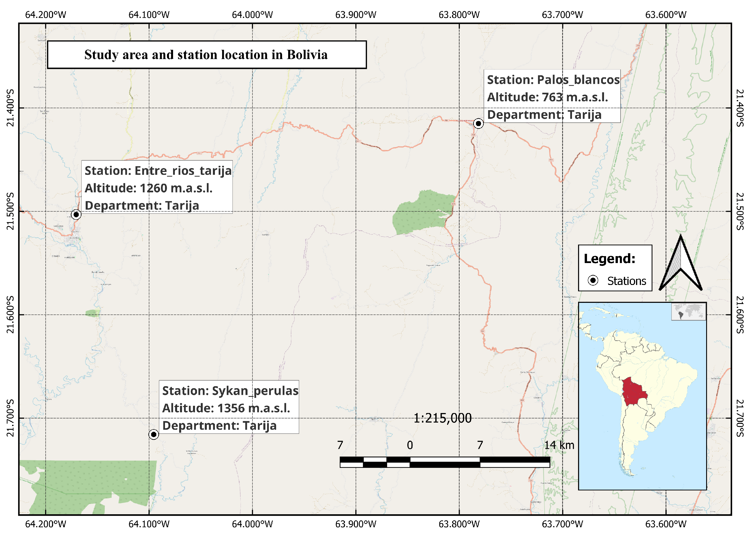
The study area is located in the valley region of Tarija, Bolivia, between latitudes 21.400° S and 21.700° S, and longitudes 64.200° W and 66.600° W, as shown in Figure 1.

Three nearby hydrological stations within the study area were selected based on data availability, with records ranging from 15 to 23 years within the period from 1 January 2001, to 30 November 2023.

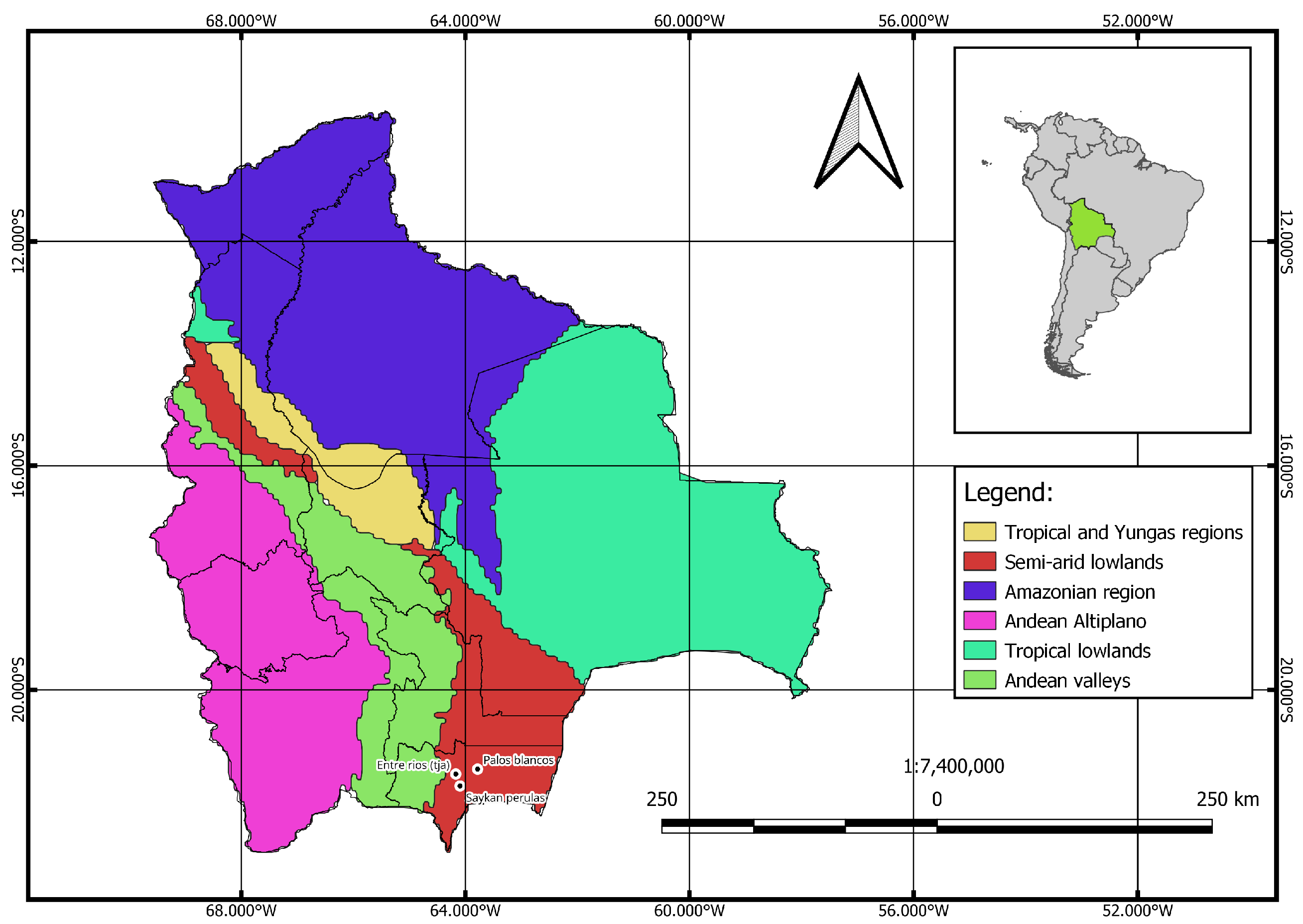
The stations are located within the semi-arid lowlands region, as shown in the classification presented in Figure 2. This area corresponds to the Tarija region. The classification is based on the approach proposed by Santos [35] and SENAMHI Bolivia, which defines clusters using precipitation, temperature, and elevation data from hydrometeorological stations across Bolivia.

For the preliminary assessment, the percentage of valid daily precipitation data (%) was calculated for each station over the selected period, following the approach of Kim [28].

The homogeneity test was performed using the double mass curve (DMC) method to verify the consistency of the data over time and to ensure that the stations did not undergo significant changes in their measurement behavior.

2.2. Methodology

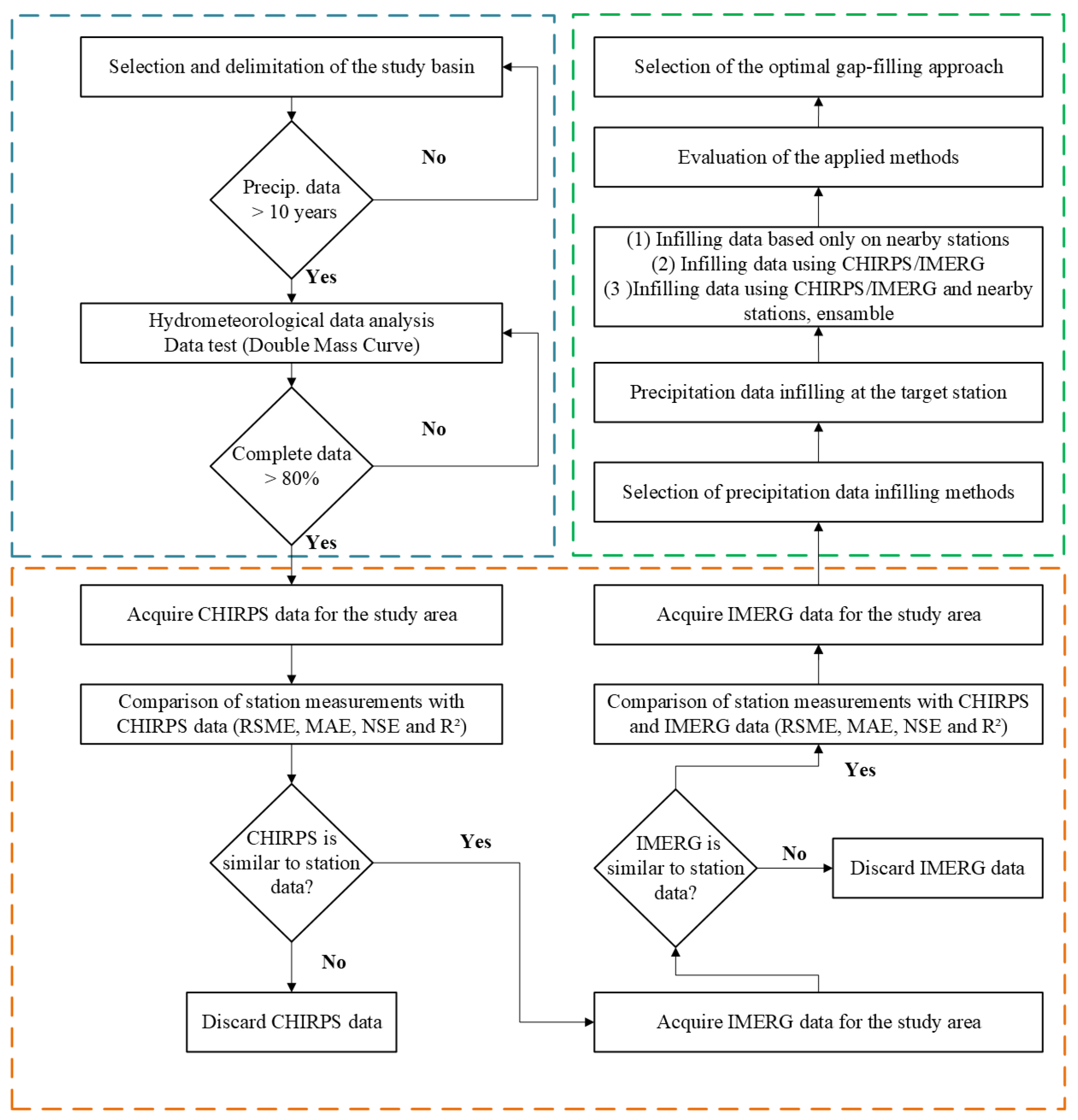
The methodology adopted follows the logic outlined in Figure 3. The first stage (indicated in blue) involves the selection of the study area, which includes hydrological stations located in close proximity to each other. These stations are required to have at least 10 years of available precipitation data and are validated through homogeneity tests.

The second stage (indicated in orange) involves acquiring CHIRPS and IMERG satellite-based precipitation data for the locations of these stations and validating them by comparing them with ground-based observations through statistical metrics.

The final stage (indicated in green) involves applying selected gap-filling methods to the station with the highest proportion of missing data. The methods utilize information from nearby stations, satellite data, and a combined ensemble of ground and satellite data, in order to evaluate which approach minimizes the uncertainty relative to the actual measured values.

2.3. CHIRPS and IMERG Data Acquisition and Validation

Daily CHIRPS precipitation data were obtained from the Climate Hazards Center at the University of California, Santa Barbara (https://www.chc.ucsb.edu, accessed on 18 February 2026) for the period spanning 1 January 2001, to 30 November 2023, with a spatial resolution of 0.05° × 0.05°. This period was selected to match the temporal coverage of the ground-based station observations used in the study.

For each meteorological station, the CHIRPS grid cell closest to the station coordinates was extracted and used as the representative satellite-derived precipitation series. As the CHIRPS product already incorporates gauge-adjustment, bias-correction, and spatial interpolation procedures [36], the dataset was used directly without further pre-processing prior to the statistical analyses.

NASA provides three main IMERG products: the Early near-real-time run, the Late run, and the Final run. All IMERG products provide global coverage between 60° N and 60° S, with a spatial resolution of 0.1° × 0.1° and a temporal resolution of 30 min [37]. In this study, the IMERG Final Run product was retrieved from the NASA Goddard Earth Sciences Data and Information Services Center (GES DISC) (https://disc.gsfc.nasa.gov/datasets/GPM_3IMERGDF_07, accessed on 28 February 2026).

Similarly, for the IMERG product, the grid cell closest to each meteorological station was extracted and used as the representative satellite-derived precipitation series. Since the Final Run product already incorporates gauge-adjustment and calibration procedures [38], the dataset was employed directly without further pre-processing prior to the statistical analyses.

To assess the reliability of satellite-based precipitation products for gap-filling purposes, a Taylor diagram based on normalized statistics was applied to both CHIRPS and IMERG datasets. This method provides a concise evaluation of agreement with ground-based observations by combining the correlation coefficient, normalized standard deviation, and centered RMSE in a single framework. The normalization allows for direct comparability by scaling variability relative to the reference data, facilitating a clear assessment of product performance.

Subsequently, a statistical comparison was conducted against ground-based station records. This validation employed key performance metrics, including the Root Mean Square Error (RMSE), the Mean Absolute Error (MAE), the Nash-Sutcliffe Efficiency coefficient (NSE) and the coefficient of determination (R²), enabling a robust evaluation of the consistency and agreement between satellite-derived and observed precipitation data.

The Root Mean Square Error (RMSE) is given by:

$$RMSE=\sqrt{{\displaystyle \frac{1}{n}}\sum _{i=1}^n{(P_i-O_i)}^2}$$

(1)

where: $P_i$ is the precipitation estimated by CHIRPS/IMERG, $O_i$ is the observed precipitation at ground stations and n is the total number of observations.

The Mean Absolute Error (MAE) is given by:

$$MAE={\displaystyle \frac{1}{n}}{\displaystyle \sum _{i=1}^n}|P_i-O_i|$$

(2)

where: $P_i$ is the precipitation estimated by CHIRPS/IMERG, $O_i$ is the observed precipitation at ground stations and n is the total number of observations.

The Nash-Sutcliffe Efficiency (NSE) coefficient is given by:

$$NSE={\displaystyle \frac{{\sum }_{i=1}^n{(P_i-O_i)}^2}{{\sum }_{i=1}^n{(O_i-{\overline{O}}_i)}^2}}$$

(3)

where: $P_i$ is the precipitation estimated by CHIRPS/IMERG, $O_i$ is the observed precipitation at ground stations, ${\overline{O}}_i$ is the mean of the observed precipitation values and n is the total number of observations.

The coefficient of determination ($R^2$) is given by:

$$R^2=1-{\displaystyle \frac{{\sum }_{i=1}^n{(O_i-P_i)}^2}{{\sum }_{i=1}^n{(O_i-\overline{O})}^2}}$$

(4)

where: $P_i$ is the precipitation estimated by CHIRPS/IMERG, $O_i$ is the observed precipitation at ground stations, $\overline{O}$ is the mean observed precipitation and n is the total number of observations.

To further evaluate the ability of the gap-filling methods to reproduce precipitation intensity patterns, contingency matrices were constructed using categorized daily precipitation values. Both observed and reconstructed precipitation series were classified into predefined intensity ranges, including no precipitation [0–1) mm, light [1–5) mm, moderate [5–20) mm, heavy [20–40) mm, and violent precipitation (≥ 40) mm events [39].

The contingency matrix allows the comparison between observed and reconstructed categories by quantifying the frequency of correctly and incorrectly classified events, providing additional insight into the performance of each method beyond continuous statistical metrics such as RMSE or NSE.

$$P_{ij}={\displaystyle \frac{n_{ij}}{{\sum }_{j=1}^k{n}_{ij}}}\times 100$$

(5)

where: $P_{ij}$ is the percentage of occurrences for category i classified as category j, $n_{ij}$ is the number of observations belonging to category i that were estimated as category j, and k is the total number of precipitation intensity categories.

2.4. Gap-Filling Precipitation Methods

The data gap-filling methods were selected based on their practicality and ease of application. These are deterministic approaches that can be applied across different contexts. The chosen methods include simple linear regression, inverse distance squared weighting, and multiple linear regression, the latter aiming to incorporate basic machine learning tools.

Linear regression ($LR$). Simple linear regression estimates the missing value based on a linear relationship with a predictor variable from a nearby station or related dataset. The model is expressed as:

$$\widehat{y}={\beta }_o+{\beta }_{1}x$$

(6)

where: $\widehat{y}$ is the estimated precipitation value for the target station, x is the observed precipitation value from the selected nearby reference station, ${\beta }_o$ is the intercept, and ${\beta }_1$ is the regression coefficient (slope), both calculated from the linear relationship between the target station and the nearest reference station using periods with concurrent observations.

Inverse Distance Squared Weighting ($ID{W}^2$). This spatial interpolation method estimates a missing value using a weighted average of neighboring stations, with weights inversely proportional to the square of the distance:

$$\widehat{y}={\displaystyle \frac{{\sum }_{i=1}^n\raisebox{1ex}{$y_i$}\!\left/ \!\raisebox{-1ex}{$d^2$}\right.}{{\sum }_{i=1}^n\raisebox{1ex}{$1$}\!\left/ \!\raisebox{-1ex}{$d_i^2$}\right.}}$$

(7)

where: $\widehat{y}$ is the estimated (filled) value, $y_i$ is the observed value at the ith neighboring station, $d_i$ is the distance between the target location, the ith station and n is the number of nearby stations used for interpolation.

Multiple Linear Regression ($MLR$). Multiple linear regression incorporates multiple predictor variables to estimate the missing value. It is defined as:

$$\widehat{y}=\beta +{\beta }_1{x}_1+{\beta }_2{x}_2+\dots +{\beta }_p{x}_p$$

(8)

where: $\widehat{y}$ is the estimated (filled) value, $x_1+x_2,\dots ,x_p$ are the predictor variables, ${\beta }_o$ is the intercept, ${\beta }_1+{\beta }_2+\dots +{\beta }_p$ are the regression coefficients estimated from historical periods with concurrent observations between the target station and the predictor datasets.

The gap-filling process for the target station was carried out using three application schemes: (i) using only nearby ground-based stations, ($ii$) using only CHIRPS or IMERG satellite data, and ($iii$) using an ensemble of both ground-based and CHIRPS or IMERG data.

These approaches were selected to evaluate how each data source contributes to reconstruction accuracy. The consistency and reliability of the reconstructed series were evaluated using RMSE and NSE to determine the most suitable approach for the conditions of the study area.

To ensure a more robust and conservative assessment, additional data gaps corresponding to the periods 2008–2010, 2015–2017, and 2021–2022 were intentionally introduced into the target station series. These continuous missing periods represent approximately 27% of the total record length, a value close to 30%.

The resulting percentage was determined by the removal of complete multi-year intervals rather than by imposing an exact proportion of missing data, thereby representing a worst-case scenario involving extended periods without available observations. Although this configuration was selected to simulate a realistic reconstruction scenario commonly encountered in sparse hydroclimatic monitoring networks, the performance of the evaluated methods may vary under different proportions or temporal distributions of missing data. Therefore, the sensitivity of the results to alternative gap patterns remains a topic for future investigation.

3. Results

3.1. Preliminary Precipitation Data Analysis

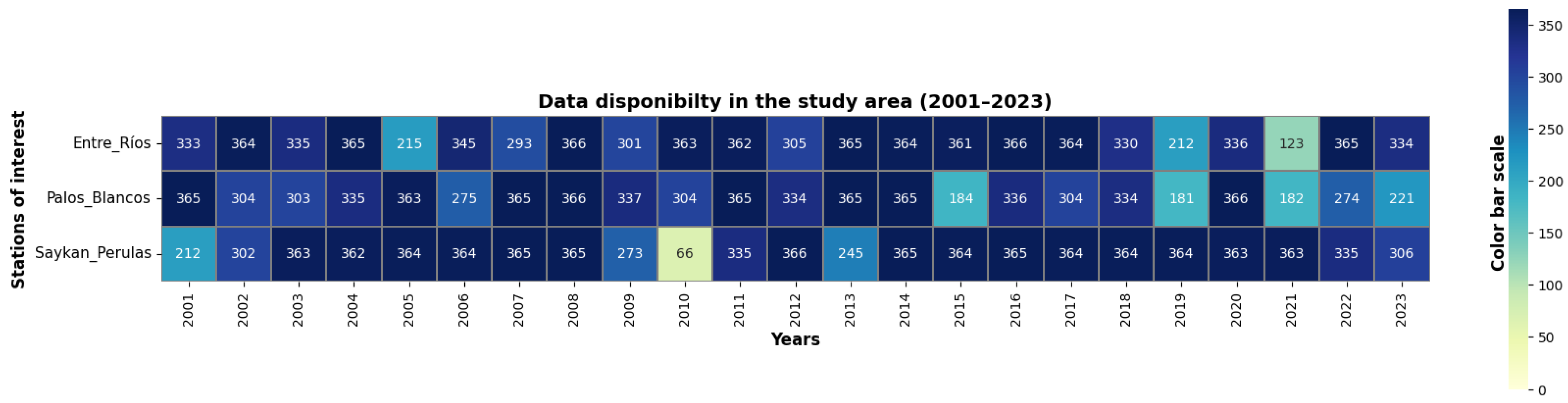
The information for this study were collected from the website of the National Service of Meteorology and Hydrology (SENAMHI accessed on 8 February 2026, https://senamhi.gob.bo). A data availability analysis was conducted, as shown in Figure 4, which displays the number of available records per station for each year. This provides a visual aid to identify the station with the least amount of available information, which will be the target station for gap-filling using data from the two closest neighboring stations as can be seen in Figure 1.

Saykan Perulas presents the longest uninterrupted gap and the highest amount of continuous missing data among the analyzed stations, with 10.3% of its records absent. Although Entre Ríos and Palos Blancos show slightly higher overall missing percentages (10.8% and 14.8%, respectively) the gaps in Saykan are more prolonged and concentrated. Due to this pattern and its strategic relevance, Saykan Perulas was selected as the target station for gap-filling, utilizing data from nearby ground stations and CHIRPS satellite estimates.

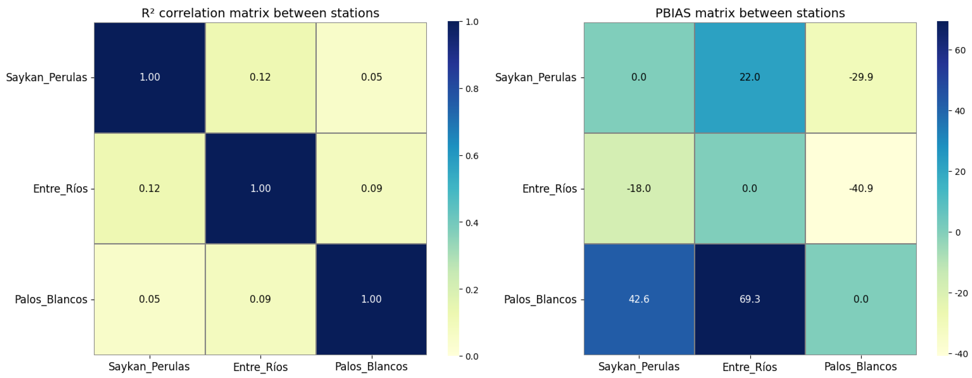
Entre Ríos was selected as the primary reference station for gap filling at Saykan Perulas due to its comparatively better statistical agreement with the target station, as can be observed in the correlation matrices shown in Figure 5. The $R^2$ value between Saykan Perulas and Entre Ríos was 0.12, higher than that obtained with Palos Blancos ($R^2=0.05$), while the PBIAS was lower (22.0% compared to $-29.9\%$). Although the stations are geographically close, the overall low correlation reflects the strong spatial variability of precipitation associated with the marked altitudinal differences in the study area, as shown in Figure 1.

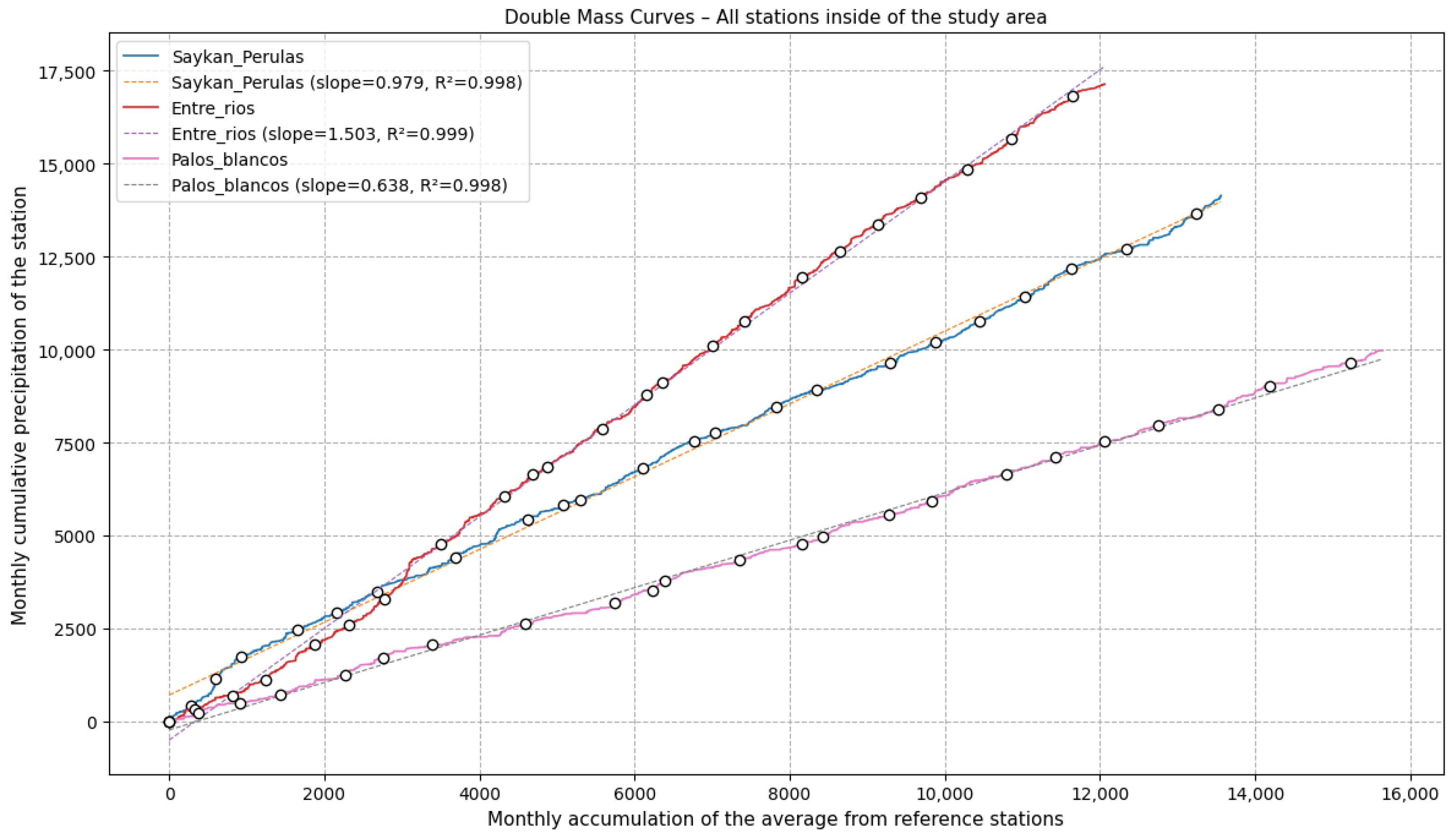
Additionally, a DMC analysis was performed for the three stations, as shown in Figure 6. The results indicate strong proportionality among the stations and high consistency, with R² values very close to 1. Therefore, the stations are considered suitable for this study, offering an extensive and consistent data record. Furthermore, no evident break-points or abrupt changes in the slope of the double mass curves were observed, suggesting the absence of major inconsistencies or long-term inhomogeneities in the precipitation records during the analyzed period.

3.2. CHIRPS and IMERG Precipitation Data Analysis

The CHIRPS and IMERG data were downloaded for the exact coordinates of the study stations using a custom Python V3.11.9 script, which is available in the GitHub repository (https://github.com/M1ch1-dev, accessed on 28 November 2025).

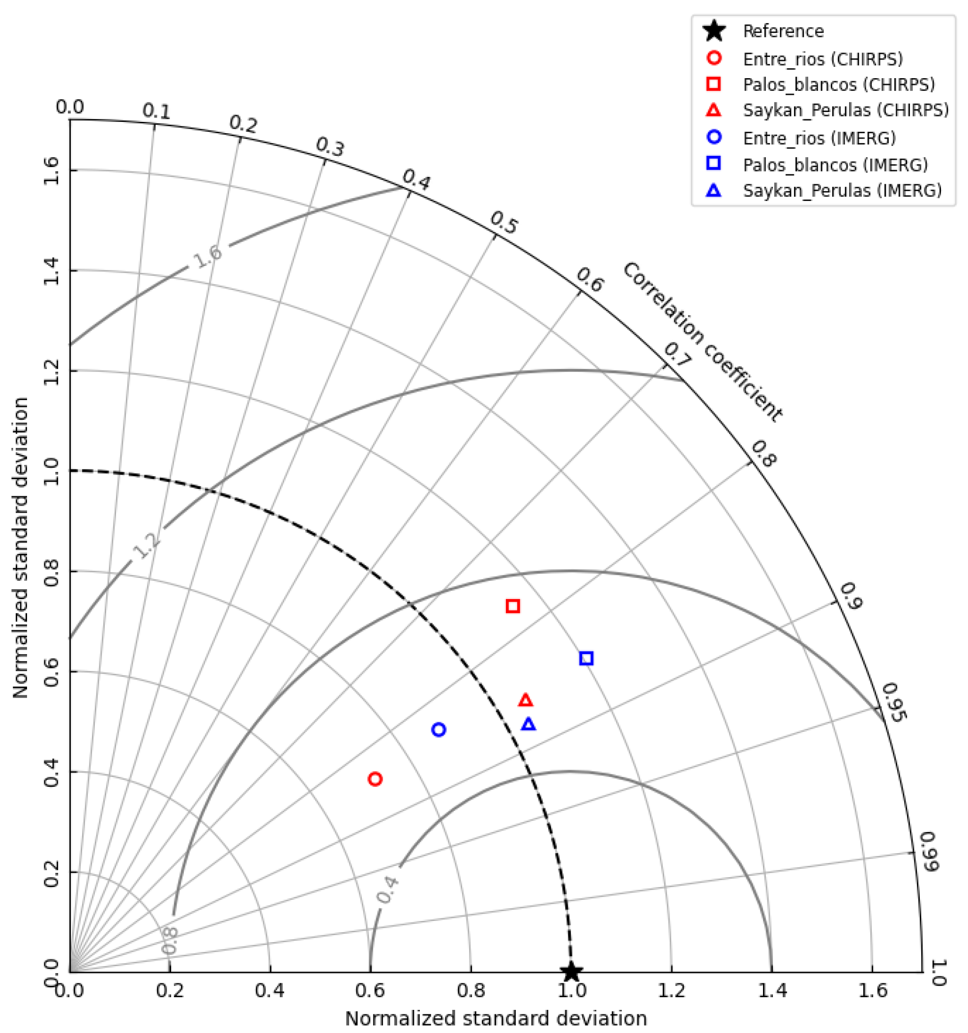
Subsequently, a comparative evaluation was conducted between the ground-based observations and the satellite-derived estimates using statistical performance metrics, including RMSE and NSE. Additionally, the Taylor diagram (Figure 7) provides a consolidated visualization of the agreement between datasets, indicating that, in general, IMERG exhibits a slightly closer correspondence to the station measurements compared to CHIRPS.

The correlation coefficients obtained for the evaluated stations (CHIRPS: 0.84, 0.77, and 0.86; IMERG: 0.83, 0.85, and 0.88) at Entre Ríos, Palos Blancos, and Saykan, respectively, are comparable, although slightly lower, than those reported by Santos [35] for GPM predecessor products (0.89, 0.83, and 0.82) at the same stations. It should be noted that Santos evaluated continuous monthly precipitation series, whereas the present study focuses on daily records, which exhibit substantially higher temporal variability. Nevertheless, the obtained correlations suggest that both satellite products are capable of reproducing the general temporal behavior of precipitation within the study area.

However, the NSE and RMSE values presented in

Table 1. Statistical performance of CHIRPS and IMERG products against raw gauge observations at daily scale within the study area.

Station Names	Dataset	R2	NSE	RMSE
Saykan Perulas	CHIRPS	0.86	−0.33	8.23
	IMERG	0.88	−0.50	8.65
Entre Rios	CHIRPS	0.84	−0.60	9.68
	IMERG	0.83	−0.65	8.77
Palos Blancos	CHIRPS	0.77	−0.01	8.66
	IMERG	0.85	−0.22	10.43

reveal important limitations in reproducing daily precipitation magnitudes and extreme rainfall events. Although both satellite products exhibited moderate-to-high correlation coefficients, the negative NSE values and RMSE ranging from 8.2 to 10.4 mm/day indicate considerable uncertainty in reproducing local precipitation dynamics. These results suggest that, under the complex topographic and climatic conditions of the study area, the satellite products are able to capture the general temporal behavior of precipitation but remain limited in accurately representing daily rainfall magnitudes and extremes.

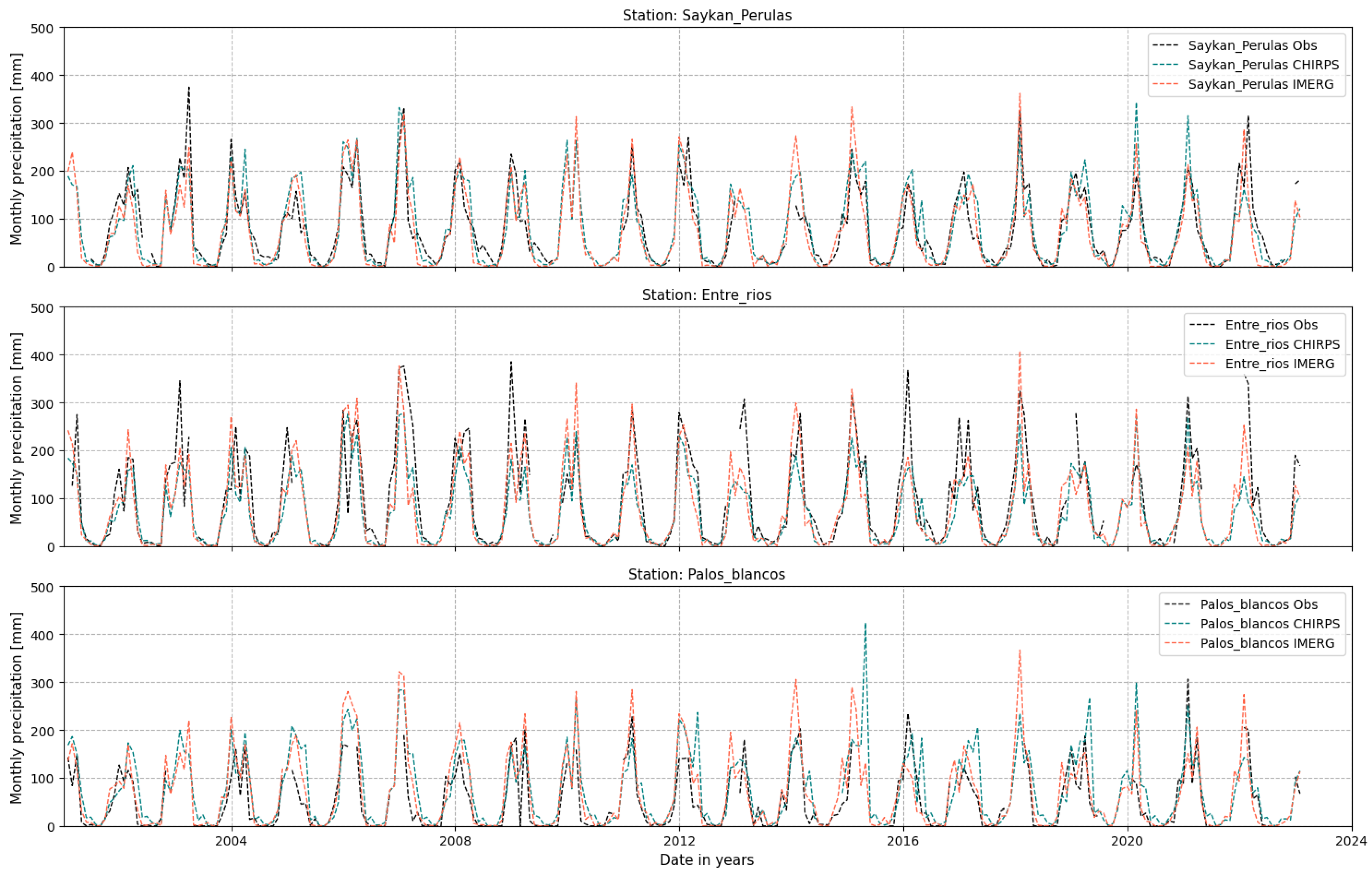
Figure 8 presents a monthly comparison between ground-based station observations and precipitation estimates derived from both CHIRPS and IMERG. The results suggest that CHIRPS tends to overestimate precipitation at two of the three stations, although it successfully reproduces the observed seasonal pattern and temporal variability. In contrast, IMERG displays a comparable seasonal behavior but yields slightly lower performance metrics at the evaluated stations.

These findings are consistent with previous studies. In Bolivia, Collarani [31] reported monthly coefficients of determination (R²) ranging from 0.42 to 0.91, which are considered acceptable at that temporal scale. Similarly, in neighboring Chile, Zambrano [40] described positive correlations, with most daily values falling between 0.2 and 0.6, and higher median values observed at monthly (0.60–0.95) timescales.

Consequently, although both datasets exhibit comparable seasonal behavior, IMERG demonstrated slightly superior performance relative to CHIRPS in terms of RMSE and Nash–Sutcliffe efficiency across the evaluated stations; therefore, both datasets were retained for subsequent analyses.

3.3. Gap-Filling Precipitation Data Analysis

3.3.1. Linear Regression (LR) Method

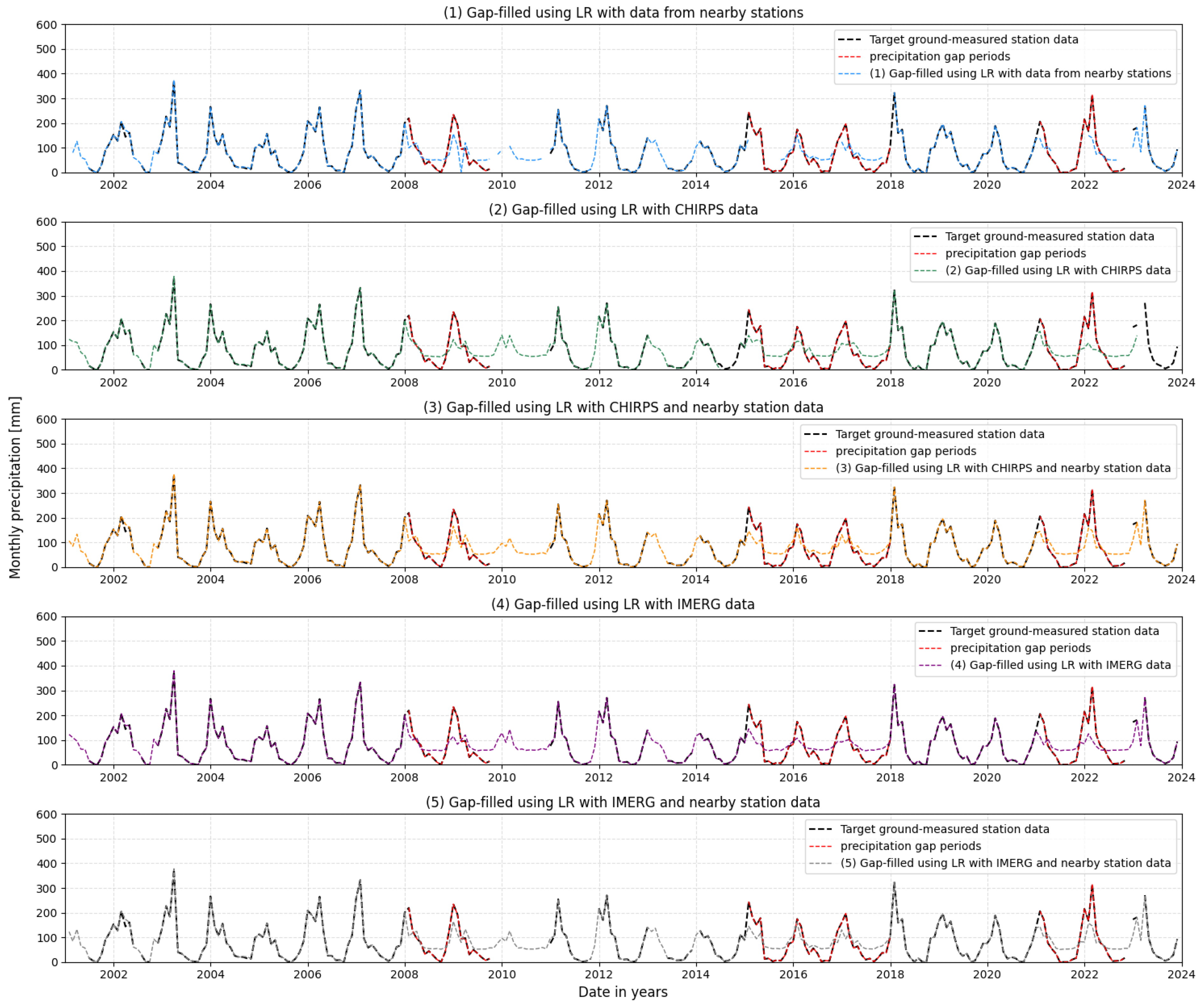
Figure 9 presents a comparison of five gap-filling approaches. (1) data from nearby stations; (2) satellite-based CHIRPS estimates in the absence of nearby stations; (3) a hybrid approach combining CHIRPS and station data; (4) satellite-based IMERG estimates in the absence of nearby stations; and (5) a hybrid approach combining IMERG and station data to construct more complete and reliable precipitation time series.

The Entre Ríos station was selected as the nearby station for simple linear regression due to its relatively higher correlation with the target station. As shown, the time series reconstructed using station-only data and the hybrid approach best reproduce the observed precipitation patterns.

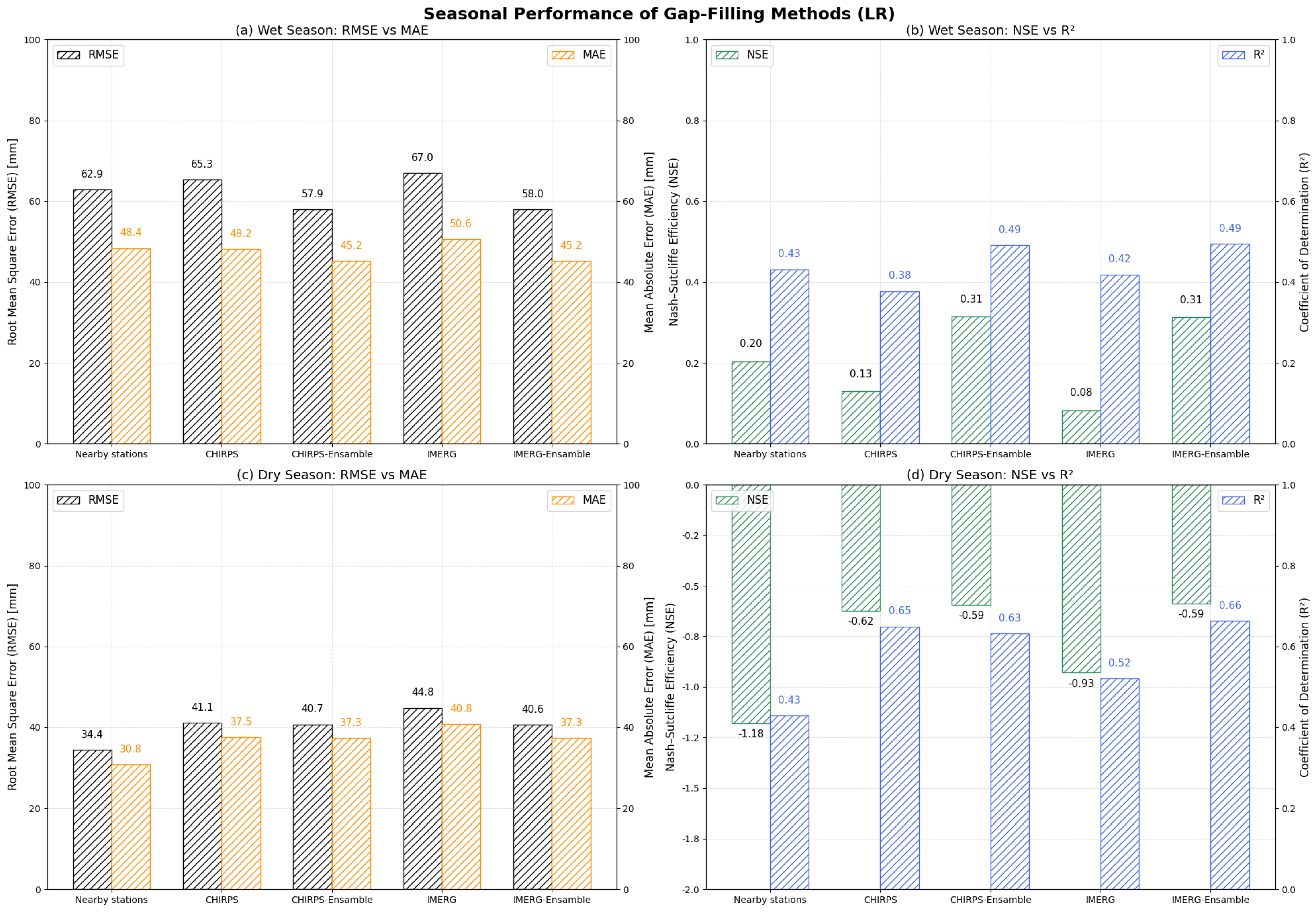
This is further supported by the seasonal statistical evaluation presented in Figure 10. During the wet season, all approaches achieved positive NSE values ranging from 0.08 to 0.31, indicating a moderate ability to reproduce the temporal variability of precipitation despite the higher rainfall magnitudes and greater event variability. The ensemble-based approaches (CHIRPS-Ensemble and IMERG-Ensemble) consistently produced the highest NSE and R² values, together with lower RMSE and MAE, demonstrating a modest but systematic improvement relative to the satellite-only implementations.

In contrast, the dry season exhibited substantially lower NSE values, which became negative for all evaluated approaches despite moderate-to-high R² coefficients (0.43–0.66). This behavior reflects the well-known sensitivity of NSE to low-variance conditions, where relatively small reconstruction errors can produce large reductions in efficiency scores. Nevertheless, the ensemble approaches maintained the highest R² values and among the lowest reconstruction errors, indicating a better representation of seasonal precipitation variability.

Overall, the performance gains obtained by incorporating satellite information remained moderate, generally improving goodness-of-fit metrics by approximately 5–15% relative to the standalone satellite approaches. Although these improvements were not dramatic, the results demonstrate that satellite-derived precipitation products can provide useful complementary information for precipitation reconstruction in regions with sparse observational networks and complex topographic conditions.

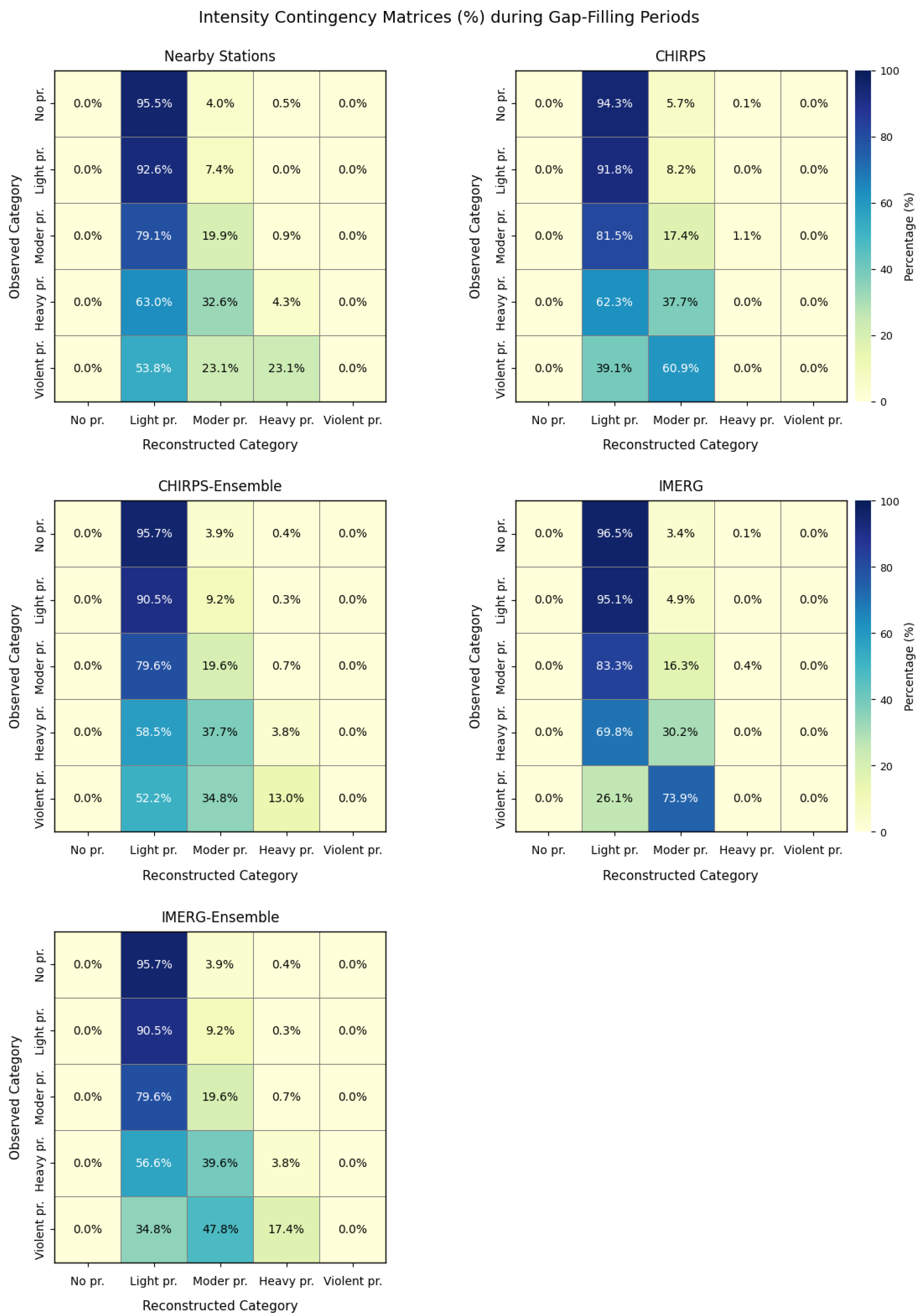
The intensity contingency matrices presented in Figure 11 reinforce the trends previously identified through the RMSE, NSE, MAE, and R² metrics. Overall, all reconstruction methods concentrated most precipitation events within the light-precipitation category, where agreement values generally exceeded 90%. This indicates that the evaluated approaches are capable of reproducing the general temporal occurrence of low-intensity rainfall events, which constitute a large proportion of the precipitation record in the study area.

However, performance decreased substantially as precipitation intensity increased. Moderate precipitation events were frequently underestimated and reclassified as light precipitation, while heavy and violent precipitation events were rarely reconstructed correctly. For instance, more than 60% of the observed heavy precipitation events were classified as light precipitation by the Nearby Stations, CHIRPS, and IMERG approaches. Similarly, violent precipitation events were predominantly reassigned to light or moderate precipitation categories, indicating limited capability in reproducing extreme daily rainfall magnitudes associated with convective rainfall processes.

These results are consistent with the seasonal performance analysis, which showed comparatively better agreement during wet-season conditions but persistent difficulties in reproducing high-intensity precipitation events. Consequently, although the evaluated methods can adequately represent the occurrence and seasonality of precipitation, substantial uncertainties remain in the reconstruction of extreme rainfall magnitudes.

Nevertheless, the matrices also reveal a systematic tendency in the LR-based approaches to smooth precipitation variability, concentrating reconstructed values within lower precipitation classes. This behavior may explain why the methods reproduce the general seasonal occurrence of precipitation reasonably well while still presenting limitations in representing the magnitude and intensity of extreme daily rainfall events during the wet season.

3.3.2. Multiple Linear Regression (MLR) Method

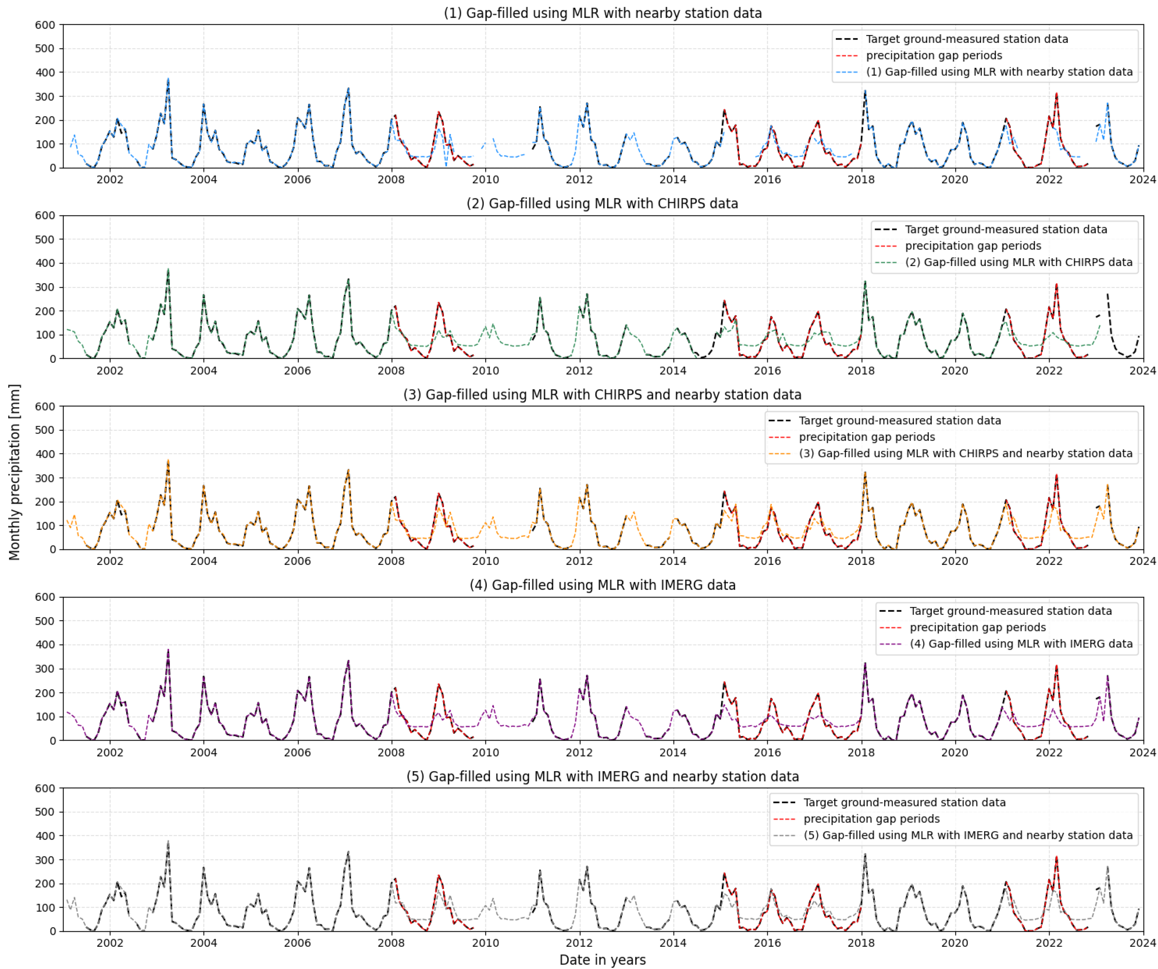
Figure 12 shows the precipitation time series reconstructed using the Multiple Linear Regression (MLR) method and the approaches (1) to (5). Although its overall temporal pattern closely resembles that obtained from simple linear regression, MLR demonstrates a slight enhancement in reconstruction accuracy, leading to a slightly better representation of the observed variability.

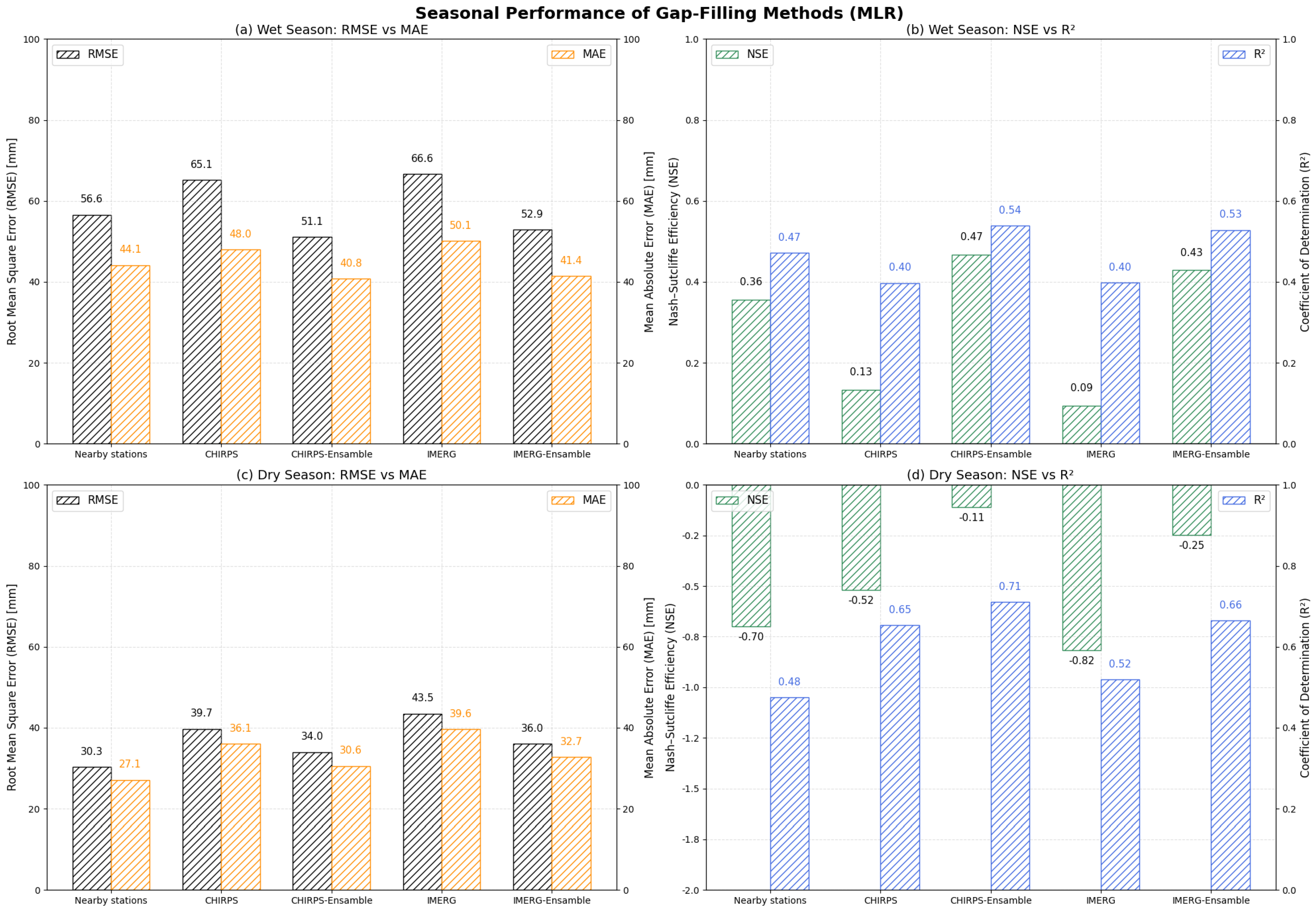
In this configuration (Figure 12), the Entre Ríos and Palos Blancos stations were incorporated as auxiliary predictors within the multiple linear regression framework. By combining information from multiple neighboring stations, the model aimed to better capture the spatial variability of precipitation across the study area, despite the relatively low inter-station correlations. As reflected by the statistical metrics shown in Figure 13, the inclusion of the additional predictor led to a slight reduction in RMSE and a modest increase in NSE compared with the simple linear regression (LR) approach, indicating a more consistent reconstruction of precipitation variability.

Overall, the MLR approach produced more consistent improvements than LR, particularly when satellite products were combined with neighboring station observations. The seasonal analysis revealed that the ensemble-based reconstructions achieved the best overall performance during both wet and dry-season conditions. During the wet season, the CHIRPS-Ensemble approach increased NSE by approximately 31% relative to the Nearby Stations method, while reducing RMSE by nearly 10%. Similarly, IMERG-Ensemble improved NSE by approximately 19% and reduced RMSE by about 7%. The ensemble approaches also increased the coefficient of determination by approximately 15–20% relative to the standalone satellite products, indicating an improved representation of precipitation variability.

Similar behavior was observed during the dry season. Although all methods produced negative NSE values, reflecting the greater difficulty of reconstructing precipitation under low-variance conditions, the ensemble approaches substantially reduced performance losses. In particular, CHIRPS-Ensemble improved NSE by approximately 79% relative to the standalone CHIRPS reconstruction and achieved the highest R² value (0.71), representing an increase of approximately 9% compared to CHIRPS alone. Likewise, IMERG-Ensemble improved NSE by approximately 70% relative to IMERG and increased R² by approximately 27%.

The standalone CHIRPS and IMERG products generally exhibited larger reconstruction errors and lower efficiency metrics than their ensemble counterparts. Nevertheless, CHIRPS consistently outperformed IMERG in most performance indicators, suggesting a better adaptation to the climatic and topographic conditions of the study area. Although the improvements obtained through the ensemble framework remained moderate overall, the results demonstrate that integrating satellite-derived precipitation products with ground-based observations provides a more reliable reconstruction strategy than using either information source independently.

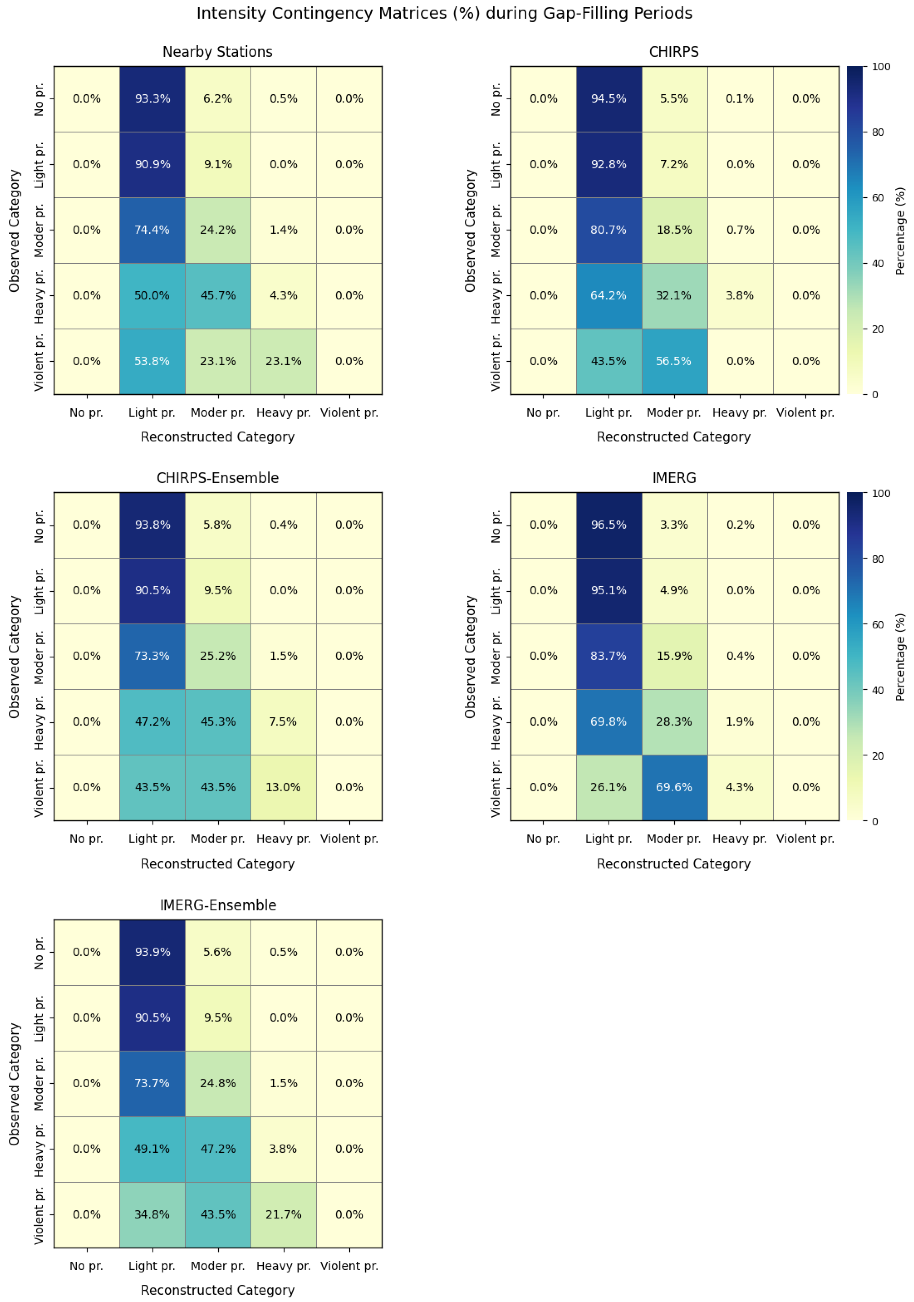
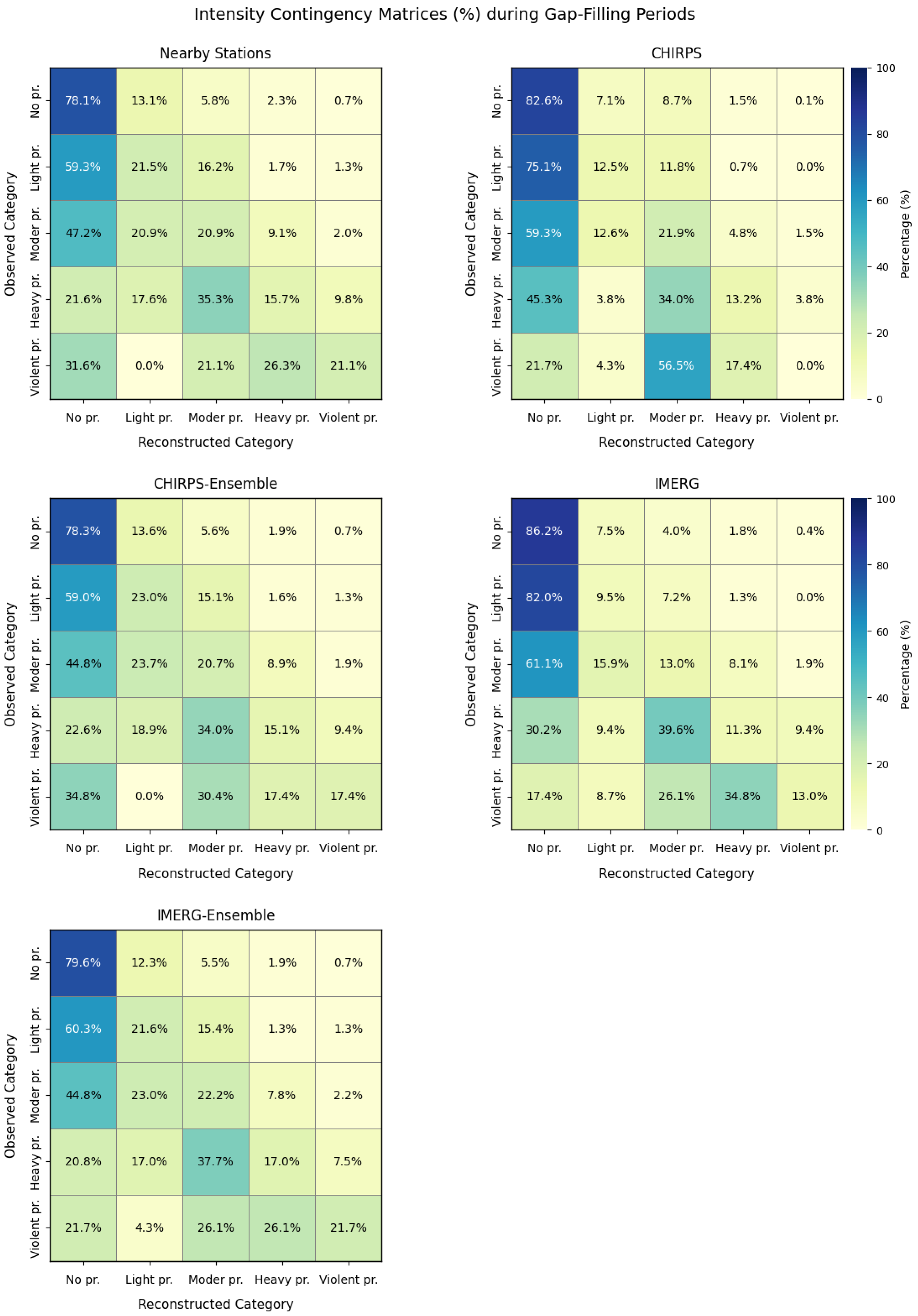
Figure 14 presents the intensity contingency matrices obtained for the evaluated MLR gap-filling approaches. Overall, all methods showed a strong concentration of reconstructed events within the light precipitation category, indicating a satisfactory representation of the general occurrence and seasonality of precipitation. This behavior is consistent with the seasonal statistical metrics, which showed better agreement for low- and moderate-intensity precipitation but persistent difficulties in reproducing extreme rainfall events.

The standalone satellite products, particularly IMERG, tended to smooth precipitation extremes by frequently classifying moderate-to-heavy precipitation as light or moderate rainfall. For example, more than 69% of the observed violent precipitation events were reconstructed as moderate precipitation by the standalone IMERG approach, whereas CHIRPS achieved a comparatively better representation of moderate precipitation categories, suggesting a stronger ability to capture local precipitation variability under the climatic and topographic conditions of the study area.

The ensemble-based approaches provided moderate improvements relative to the standalone satellite products by increasing the proportion of correctly reconstructed medium- and high-intensity precipitation events and reducing their misclassification into lower precipitation categories. Nevertheless, all methods continued to underestimate violent precipitation events, reflecting the difficulty of reproducing highly localized convective rainfall processes. Overall, the MLR-based reconstructions more closely approximated the observed precipitation patterns than the LR models, suggesting that the incorporation of multiple predictors partially mitigates the smoothing effect associated with simpler regression approaches. In particular, the superior performance of the CHIRPS–Ensemble method further highlights the potential value of CHIRPS data for precipitation reconstruction in regions with sparse observational networks.

3.3.3. Inverse Distance Weight Square (IDW²) Method

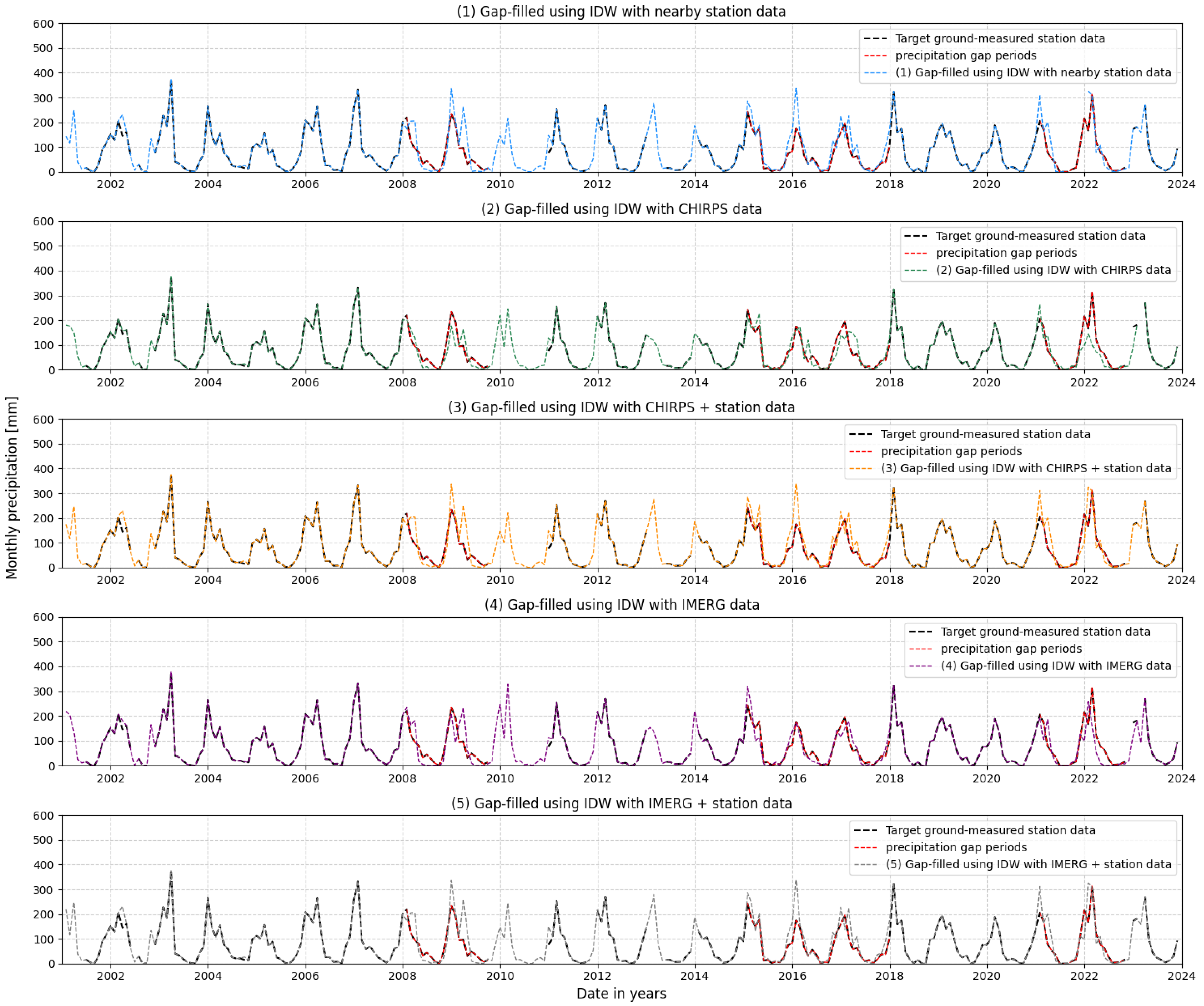
Figure 15 presents the comparison of approaches (1) to (5) using the IDW method. It can be observed that this technique performs the poorest in reproducing actual precipitation measurements from nearby ground stations.

The reconstructed series often diverges from the observed precipitation patterns, making IDW the least accurate and reliable method among those evaluated. Interestingly, when applied solely to CHIRPS and IMERG data, IDW appears to perform relatively better. This improvement does not imply that IDW more accurately represents the true precipitation, but rather that the spatially consistent and smoothed nature of CHIRPS data reduces the impact of local errors.

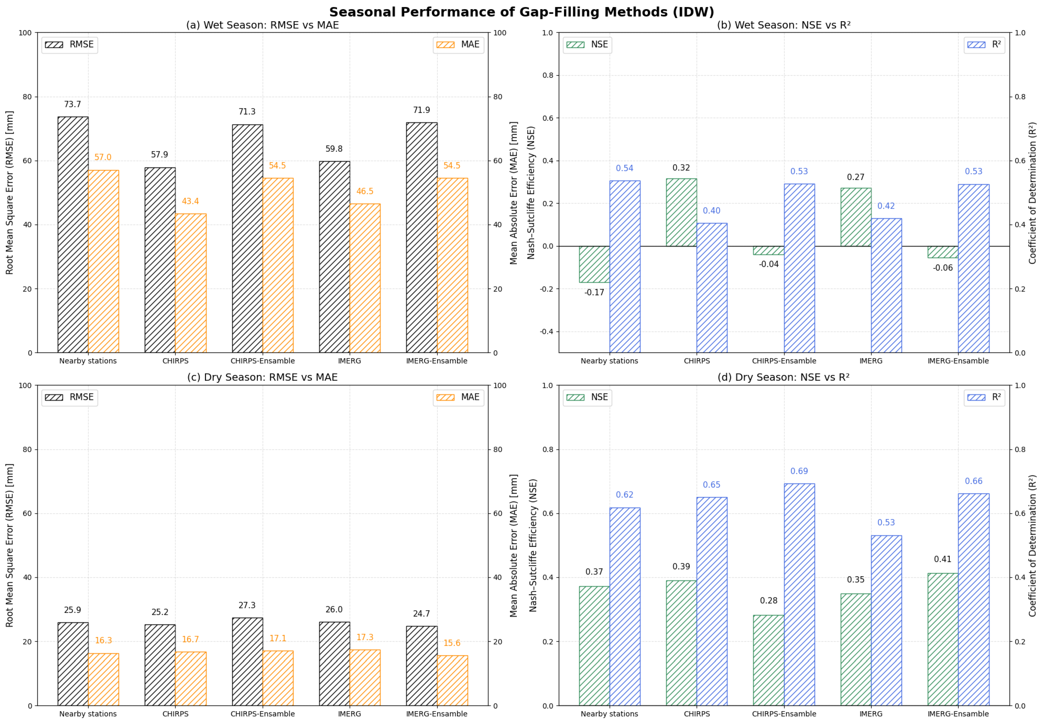
The seasonal statistical metrics presented in Figure 16 highlight the strong dependence of the IDW performance on precipitation regime. During the wet season, all approaches exhibited substantially larger reconstruction errors, with RMSE values ranging from 57.9 to 73.7 mm and MAE values between 43.4 and 57.0 mm. In contrast, dry-season errors were considerably lower, with RMSE values of approximately 25–27 mm and MAE values of 15–17 mm, reflecting the lower precipitation variability characteristic of this period.

Among the evaluated approaches, the standalone CHIRPS product achieved the best overall performance during the wet season, presenting the lowest RMSE (57.9 mm), lowest MAE (43.4 mm), and highest NSE (0.32). Conversely, the nearby-station and ensemble-based implementations generally showed weaker performance, suggesting that the incorporation of additional predictors did not consistently improve the spatial interpolation results under high-rainfall conditions.

The NSE results further reveal the limitations of the IDW approach. Several methods produced negative NSE values during the wet season, indicating that the reconstructed series performed worse than using the observed seasonal mean as a predictor. However, all approaches yielded positive NSE values during the dry season, ranging from 0.28 to 0.41, demonstrating a better capability to reproduce precipitation variability under lower-intensity rainfall conditions.

These results suggest that the performance of IDW is strongly affected by the pronounced spatial heterogeneity of precipitation within the study area. Since the method relies exclusively on distance-based weighting, it is unable to adequately represent localized convective rainfall events and complex topographic influences during the wet season. Consequently, although IDW can provide reasonable reconstructions under relatively stable dry-season conditions, its applicability becomes more limited during periods characterized by intense and spatially variable precipitation.

Figure 17 further confirms these limitations through the intensity contingency matrices.

Overall, the IDW reconstructions showed a tendency to overclassify precipitation events into the no-precipitation and light-precipitation categories while underrepresenting moderate and heavy rainfall events. This behavior was particularly evident during wet-season conditions, when the method struggled to reproduce high-intensity precipitation associated with convective rainfall processes. A substantial proportion of the observed violent precipitation events were reconstructed as moderate precipitation, indicating a tendency of the IDW approach to smooth extreme rainfall magnitudes despite preserving part of their occurrence.

Nevertheless, the seasonal analysis suggests that IDW performed comparatively better during dry-season conditions, when precipitation amounts are generally lower and spatial gradients are less pronounced. Under these conditions, the method reproduced no-precipitation and low-intensity rainfall categories more consistently, which is reflected by the lower RMSE and MAE values and the positive NSE coefficients obtained during the dry season. Interestingly, IDW also exhibited a comparatively better representation of violent precipitation events than the regression-based approaches, correctly reconstructing approximately 21.7% of the observed extreme rainfall cases, whereas LR and MLR showed very limited agreement for this category. This behavior suggests that, unlike the regression-based methods, IDW preserves part of the local precipitation variability associated with extreme events. However, this advantage is accompanied by larger overall uncertainties and stronger misclassification across intermediate precipitation categories, particularly during wet-season conditions characterized by rapid rainfall transitions and high spatial variability.

4. Conclusions

The selected study area represents a hydrologically relevant macroregion of southern Bolivia characterized by complex topographic conditions, strong spatial precipitation variability, and limited meteorological coverage. To ensure a minimum level of data reliability, only stations with less than 20.

The inclusion of CHIRPS and IMERG satellite-derived precipitation products provided a valuable complementary source of information for precipitation gap-filling. CHIRPS (0.05° × 0.05°) generally outperformed IMERG (0.1° × 0.1°), likely due to its finer spatial resolution and improved representation of local precipitation variability under the topographic conditions of the study area. Although both satellite products showed limitations in reproducing extreme daily rainfall events, their overall performance remained comparable to the station-only approaches for several evaluation metrics. Despite the relatively low and occasionally negative NSE values observed for some standalone satellite reconstructions, their moderate-to-high correlation coefficients indicate an ability to reproduce the general temporal behavior of precipitation. Consequently, their primary contribution lies not in replacing ground observations, but in providing complementary information capable of supporting precipitation reconstruction in regions with sparse observational networks.

Among the evaluated gap-filling methods, the ensemble-based approaches generally produced the best overall performance, particularly when combining CHIRPS data with nearby ground-based observations through MLR. The hybrid methods achieved consistent improvements in RMSE, MAE, NSE, and R² relative to the standalone satellite products. Although these gains were generally modest, they demonstrate the added value of integrating satellite and ground-based information. Seasonal analyses revealed contrasting performance patterns between wet- and dry-season conditions. RMSE and MAE values were generally lower during the dry season due to the reduced precipitation amounts, whereas NSE values tended to improve during the wet season, indicating a better representation of precipitation variability despite larger absolute reconstruction errors. Overall, the regression-based approaches were able to reproduce the seasonal occurrence and temporal variability of precipitation reasonably well, but still exhibited difficulties in accurately representing extreme daily rainfall events across both seasons, with the largest discrepancies occurring during humid-season periods characterized by intense convective precipitation and greater rainfall variability.

The IDW approach showed the lowest overall performance among the evaluated methods, particularly in reproducing intermediate precipitation categories and temporal precipitation variability. Nevertheless, the seasonal analysis indicated comparatively better performance during dry-season conditions, when precipitation amounts are generally lower and spatial gradients are less pronounced. Furthermore, the contingency matrix analysis revealed a comparatively better representation of certain extreme precipitation events relative to the regression-based approaches, suggesting that spatial interpolation techniques may preserve part of the local rainfall variability associated with highly convective conditions. However, these improvements were accompanied by larger overall uncertainties and stronger misclassification across intermediate precipitation categories, particularly during wet-season periods characterized by high precipitation variability, limiting the overall reliability of the method.

Overall, the results indicate that the integration of satellite-derived precipitation products with ground-based observations can contribute to improving the continuity and reconstruction of precipitation records in data-scarce regions. Although the improvements obtained through the ensemble approaches were generally modest, ranging from approximately 5% to 10% for several performance metrics, the proposed framework demonstrated greater robustness during wet-season conditions, when precipitation variability is highest and accurate reconstruction becomes more challenging. The seasonal evaluation also highlighted persistent limitations in reproducing high-intensity rainfall events associated with convective precipitation processes.

The applicability of the proposed framework to other regions should be considered in the context of local observational availability, climatic conditions, and network density. Because the present study relied on only three meteorological stations, the performance of the evaluated methods may be influenced by the sparse monitoring network and the relatively low inter-station correlations observed in the study area. Consequently, the transferability of the methodology to regions with different climatic regimes, station densities, or topographic characteristics should be assessed carefully.

Finally, although the reconstructed precipitation series were evaluated using multiple statistical and categorical performance metrics, the uncertainty associated with the reconstructed values was not explicitly quantified. Therefore, the reported results should be interpreted considering the potential uncertainty arising from observational errors, satellite-product biases, model assumptions, and the limited density of the available monitoring network. Future studies should incorporate uncertainty assessment techniques, such as bootstrap resampling, Monte Carlo simulations, or confidence-interval estimation, to quantify the uncertainty associated with reconstructed precipitation series and provide a more comprehensive characterization of reconstruction reliability for hydrological and climatological applications.

References

1. Han, H.; Kim, B.; Kim, K.; Kim, D.; Kim, H.S. Machine learning approach for the estimation of missing precipitation data: A case study of South Korea. Water Sci. Technol. 2023, 88, 556–571. [Google Scholar] [CrossRef]
2. Haidar, A.; Verma, B.; Sinba, T. A Novel Approach for Optimizing Ensemble Components in Rainfall Prediction. In Proceedings of the IEEE Congress on Evolutionary Computation (CEC); Institute of Electrical and Electronics Engineers: Piscataway, NJ, USA, 2018; pp. 1–8. [Google Scholar] [CrossRef]
3. Ochoa, C.G.; Briceño, N.; Zimmermann, E.; Vives, L.; Blanco, M.; Cazenave, G.; Ares, G. Filling Series of Daily Precipitation for Long Periods of Time in Plain Areas. Case Study Superior Basin of Stream del Azul; Asociación Argentina de Geofísicos y Geodestas: Buenos Aires, Argentina, 2017; pp. 38–60. [Google Scholar]
4. da Silva Jale, J.; Júnior, S.F.A.X.; Fialho Morais Xavier, É.; Stošić, T.; Stošić, B.; Ferreira, T.A.E. Application of markov chain on daily rainfall data in Paraíba-Brazil from 1995–2015. Acta Sci.-Technol. 2019, 41, e37186. [Google Scholar] [CrossRef]
5. Lizarazu Rojas, M.D.; Ochoa, W.A.A.; Montenegro Terrazas, L.E.; Andrade Uzieda, M.; Calabokis, O.P.; Nuñez de la Rosa, Y.E.; Nava Sejas, J.E. An Application of the RegCM4 System to Quantify the Effects of Climate Change on the Hydric Potential of the Angostura-Bolivia Basin. Water 2024, 16, 1147. [Google Scholar] [CrossRef]
6. Portuguez-maurtua, M.; Arumi, J.L.; Lagos, O.; Stehr, A.; Arquiñigo, N.M. Filling Gaps in Daily Precipitation Series Using Regression and Machine Learning in Inter-Andean Watersheds. Water 2022, 14, 1799. [Google Scholar] [CrossRef]
7. Du, H.; Tan, M.L.; Zhang, F.; Chun, K.P.; Li, L.; Kabir, M.H. Evaluating the effectiveness of CHIRPS data for hydroclimatic studies. Theor. Appl. Climatol. 2024, 155, 1519–1539. [Google Scholar] [CrossRef]
8. Rivera, J.A.; Marianetti, G.; Hinrichs, S. Validation of CHIRPS precipitation dataset along the Central Andes of Argentina. Atmos. Res. 2018, 213, 437–449. [Google Scholar] [CrossRef]
9. Papailiou, I.; Spyropoulos, F.; Trichakis, I.; Karatzas, G.P. Artificial Neural Networks and Multiple Linear Regression for Filling in Missing Daily Rainfall Data. Water 2022, 14, 2892. [Google Scholar] [CrossRef]
10. Brath, A.; Montanari, A.; Toth, E. Analysis of the effects of different scenarios of historical data availability on the calibration of a spatially-distributed hydrological model. J. Hydrol. 2004, 291, 232–253. [Google Scholar] [CrossRef]
11. Dura, J.D.P. Red neuro-difusa para el relleno de datos faltantes en la estación meteorológica Chapingo. Rev. Iberoam. Cienc. Comput. Inf. Tica 2015, 4, 1–21. [Google Scholar] [CrossRef]
12. Lucio, P.S.; Conde, F.C.; Cavalcanti, I.F.A.; Serrano, A.I.; Ramos, A.M.; Cardoso, A.O. Spatiotemporal monthly rainfall reconstruction via artificial neural network-case study: South of Brazil. Adv. Geosci. 2007, 10, 67–76. [Google Scholar] [CrossRef]
13. Aguilera, H.; Guardiola-Albert, C.; Serrano-Hidalgo, C. Estimating extremely large amounts of missing precipitation data. J. Hydroinformatics 2020, 22, 578–592. [Google Scholar] [CrossRef]
14. Shen, Z.; Yong, B.; Gourley, J.J.; Qi, W.; Lu, D.; Liu, J.; Ren, L.; Hong, Y.; Zhang, J. Recent global performance of the Climate Hazards group Infrared Precipitation (CHIRP) with Stations (CHIRPS). J. Hydrol. 2020, 591, 125284. [Google Scholar] [CrossRef]
15. Rojas, Y.; Minder, J.R.; Campbell, L.S.; Massmann, A.; Garreaud, R. Assessment of GPM IMERG satellite precipitation estimation and its dependence on microphysical rain regimes over the mountains of south-central Chile. Atmos. Res. 2021, 253, 105454. [Google Scholar] [CrossRef]
16. da Silva, L.d.D.d.J.; Mahmoud, M.; González-Rodríguez, L.; Mohammed, S.; Rodríguez-López, L.; Arias, M.I.A. Assessment of the IMERG Early-Run Precipitation Estimates over South American Country of Chile. Remote Sens. 2023, 15, 573. [Google Scholar] [CrossRef]
17. Abebe, A.J.; Solomatine, D.P.; Venneker, R.G. Application de modèles basés sur la logique floue adaptative pour la reconstitution d’événements de précipitation manquants. Hydrol. Sci. J. 2000, 45, 425–436. [Google Scholar] [CrossRef][Green Version]
18. Acock, M.C.; Pachepsky, Y.A. Estimating Missing Weather Data for Agricultural Simulations Using Group Method of Data Handling. J. Appl. Meteorol. 1999, 39, 1176–1184. [Google Scholar]
19. Xia, Y.; Fabian, P.; Stohl, A.; Winterhalter, M. Forest climatology: Estimation of missing values for Bavaria, Germany. Agric. For. Meteorol. 1999, 96, 131–144. [Google Scholar] [CrossRef]
20. Willmott, C.J.; Robeson, S.M.; Feddema, J.J. Estimating continental and terrestrial precipitation averages from rain-gauge networks. Int. J. Climatol. 1994, 14, 403–414. [Google Scholar] [CrossRef]
21. Herschy, R.; Marsh, T.; Herschy, R.; Schumann, A. Thiessen polygon. In Encyclopedia of Hydrology and Water Resources; Springer: Dordrecht, The Netherlands, 1998; pp. 648–649. [Google Scholar]
22. Buishand, T.A.; Brandsma, T. Multisite simulation of daily precipitation and temperature in the Rhine basin by nearest-neighbor resampling. Water Resour. Res. 2001, 37, 2761–2776. [Google Scholar] [CrossRef]
23. Teegavarapu, R.S.; Chandramouli, V. Improved weighting methods, deterministic and stochastic data-driven models for estimation of missing precipitation records. J. Hydrol. 2005, 312, 191–206. [Google Scholar] [CrossRef]
24. Lu, G.Y.; Wong, D.W. An adaptive inverse-distance weighting spatial interpolation technique. Comput. Geosci. 2008, 34, 1044–1055. [Google Scholar] [CrossRef]
25. Franklin, M.; Kotamarthi, V.R.; Stein, M.; Cook, D.R. Generating data ensembles over a model grid from sparse climate point measurements. J. Phys. Conf. Ser. 2008, 125, 012019. [Google Scholar] [CrossRef]
26. Ramos-Calzado, P.; Gómez-Camacho, J.; Pérez-Bernal, F.; Pita-López, M.F. A novel approach to precipitation series completion in climatological datasets: Application to Andalusia. Int. J. Climatol. 2008, 28, 1525–1534. [Google Scholar] [CrossRef]
27. Filippini, F.; Galliani, G.; Pomi, L. The estimation of missing meteorological data in a network of automatic stations. WIT Trans. Ecol. Environ. 1994, 4, 1–9. [Google Scholar]
28. Kim, J.W.; Pachepsky, Y.A. Reconstructing missing daily precipitation data using regression trees and artificial neural networks for SWAT streamflow simulation. J. Hydrol. 2010, 394, 305–314. [Google Scholar] [CrossRef]
29. Fagandini, C.; Todaro, V.; Tanda, M.G.; Pereira, J.L.; Azevedo, L.; Zanini, A. Missing Rainfall Daily Data: A Comparison Among Gap-Filling Approaches. Math. Geosci. 2023, 56, 191–217. [Google Scholar] [CrossRef]
30. Abdel-Aal, R.; Elhadidy, M. Modeling and Forecasting the Daily Maximum Temperature Using Abductive Machine Learning. Energy Res. Lab. 1995, 10, 310–325. [Google Scholar] [CrossRef]
31. Anagua, F.C.; Gómez, M.F.V. Validación del Satélite Meteorológico chirps en la cuenca rurrenabaque-bolivia. In Proceedings of the XXVIII Congreso Latinoamericano de Hidráulica Buenos Aires. XXVIII Congreso Latinoamericano de Hidráulica Buenos Aires, Buenos Aires, Argentina, 18–21 September 2018; pp. 1–9. [Google Scholar]
32. Fernanda, C.; Teixeira-Gandra, A.; Bacelar, L. Cadeia de Markov no preenchimento de falhas de dados diários de precipitação no Rio Grande do Sul. Magistra 2016, 28, 157–167. [Google Scholar]
33. Hu, Y.M.; Liang, Z.M.; Li, B.Q.; Yu, Z.B. Uncertainty assessment of hydrological frequency analysis using bootstrap method. Math. Probl. Eng. 2013, 2013, 724632. [Google Scholar] [CrossRef]
34. Villazón, M.F.; Medrano, S.C. Relleno de datos en registros de precipitación para su aplicación en modelos de simulación hidrológica. Caso de estudio: Pilcomayo-bolivia. In Proceedings of the XVI Congreso Boliviariano de Ingeniería Sanitaria, Medio Ambiente y Energias Renovables. Medio Ambiente y Energias Renovables, Santa Cruz de la Sierra, Bolivia, 15–17 October 2015; pp. 1–7. [Google Scholar]
35. Santos Cordero, C. Análisis y Evaluación de los Datos de Precipitación de los Satélites TRMM y GPM, en las 4 Macro Regiones Climáticas de Bolivia. Ph.D. Thesis, Universidad Mayor de San Andres, La Paz, Bolivia, 2016. [Google Scholar]
36. Funk, C.; Peterson, P.; Landsfeld, M.; Pedreros, D.; Verdin, J.; Shukla, S.; Husak, G.; Rowland, J.; Harrison, L.; Hoell, A.; et al. The climate hazards infrared precipitation with stations—A new environmental record for monitoring extremes. Sci. Data 2015, 2, 150066. [Google Scholar] [CrossRef] [PubMed]
37. Mahmoud, M.T.; Al-Zahrani, M.A.; Sharif, H.O. Assessment of global precipitation measurement satellite products over Saudi Arabia. J. Hydrol. 2018, 559, 1–12. [Google Scholar] [CrossRef]
38. Huffman, G.J.; Bolvin, D.T.; Nelkin, E.J.; Tan, J. Integrated Multi-SatellitE Retrievals for GPM (IMERG) Technical Documentation; Technical Report; Mesoscale Atmospheric Processes Laboratory, NASA Goddard Space Flight Center: Greenbelt, MD, USA, 2019. [Google Scholar]
39. Pérez-Montiel, J.I.; Epiayu, A.M.C.; Moscote, C.D. Evaluation of satellite precipitation products across climatic and topographic gradients in a basin in Northern South America. Environ. Chall. 2026, 22, 101426. [Google Scholar] [CrossRef]
40. Zambrano-Bigiarini, M.; Nauditt, A.; Birkel, C.; Verbist, K.; Ribbe, L. Temporal and spatial evaluation of satellite-based rainfall estimates across the complex topographical and climatic gradients of Chile. Hydrol. Earth Syst. Sci. 2017, 21, 1295–1320. [Google Scholar] [CrossRef]
Figure 1. Map of the study area in the valley region of Tarija, Bolivia, showing the location of all selected precipitation stations.
Water 18 01672 g001
Figure 2. Hydroclimatic clustering of Bolivia and spatial distribution of the selected meteorological stations across the identified macroregions.
Water 18 01672 g002
Figure 3. Flowchart illustrating the methodological framework, including station selection and validation, CHIRPS data acquisition and comparison, and the application of gap-filling techniques.
Water 18 01672 g003
Figure 4. Annual number of days with recorded precipitation availability across all stations within the study period, visualized using a color scale.
Water 18 01672 g004
Figure 5. Correlation matrix between the selected meteorological stations based on R2 and PBIAS metrics. The color scale represents the strength of agreement between station pairs.
Water 18 01672 g005
Figure 6. Monthly Cumulative Precipitation Comparison Using Double Mass Curves. The solid blue line represents the “Saykan Perulas” station, the solid red line corresponds to the “Entre Ríos” station, and the solid pink line represents the “Palos Blancos” station.
Water 18 01672 g006
Figure 7. Taylor diagram of CHIRPS and IMERG precipitation estimates relative to ground-based observations, showing correlation, normalized standard deviation, and RMSE.
Water 18 01672 g007
Figure 8. Comparative Analysis of CHIRPS Satellite-based Precipitation Estimates and Ground-based Monthly Observations (2001–2023) in the Study Area.
Water 18 01672 g008
Figure 9. Comparative analysis of LR-based gap-filling methods applied to incomplete ground-based monthly precipitation records (2001–2023) at the Saykan Perulas station, using neighboring station data (Entre rios station), CHIRPS, IMERG, and their ensemble-based predictors.
Water 18 01672 g009
Figure 10. Statistical performance of the linear regression (LR) gap-filling approach applied to the target station “Saykan Perulas” using “Entre Ríos” as the reference station. The evaluation metrics include RMSE (black lines), NSE (green lines), MAE (orange lines), and R2 (blue lines).
Water 18 01672 g010
Figure 11. Intensity contingency matrices (%) comparing observed and reconstructed (LR) daily precipitation categories during the gap-filling evaluation periods. Rows represent the observed precipitation classes, while columns correspond to the reconstructed classes.
Water 18 01672 g011
Figure 12. Comparative analysis of MLR-based gap-filling methods applied to incomplete ground-based monthly precipitation records (2001–2023) at the Saykan Perulas station, using Palos Blancos and Entre rios as the nearby stations data, CHIRPS, IMERG, and their ensemble-based predictors.
Water 18 01672 g012
Figure 13. Statistical performance of the Multiple linear regression (MLR) gap-filling approach applied to the target station “Saykan Perulas” using “Entre Ríos” and “Palos Blancos” as the reference station. The evaluation metrics include RMSE (black lines), NSE (green lines), MAE (orange lines), and R2 (blue lines).
Water 18 01672 g013
Figure 14. Intensity contingency matrices (%) comparing observed and reconstructed (MLR) daily precipitation categories during the gap-filling evaluation periods. Rows represent the observed precipitation classes, while columns correspond to the reconstructed classes.
Water 18 01672 g014
Figure 15. Comparative analysis of IDW2-based gap-filling methods applied to incomplete ground-based monthly precipitation records (2001–2023) at the Saykan Perulas station, using Palos Blancos and Entre rios as the nearby stations data, CHIRPS, IMERG, and their ensemble-based predictors.
Water 18 01672 g015
Figure 16. Statistical performance of the IDW2 gap-filling approach applied to the target station “Saykan Perulas” using “Entre Ríos” and “Palos Blancos” as the reference station. The evaluation metrics include RMSE (black lines), NSE (green lines), MAE (orange lines), and R2 (blue lines).
Water 18 01672 g016
Figure 17. Intensity contingency matrices (%) comparing observed and reconstructed (IDW2) daily precipitation categories during the gap-filling evaluation periods. Rows represent the observed precipitation classes, while columns correspond to the reconstructed classes.
Water 18 01672 g017