Rapid Prediction of Typhoon-Induced Tidal-Flat Morphodynamics Using an Observation-Supported Deep Learning Emulator

Abstract

Tidal-flat changes during typhoon events are controlled by compound interactions among waves, tides, runoff, sediment transport, and vegetation resistance. However, rapid prediction remains challenging because high-resolution process-based morphodynamic models are computationally expensive. This study developed an observation-supported coastal morphodynamic emulator for rapid prediction of typhoon-induced tidal-flat erosion and deposition in the Jiuduansha Wetland, Yangtze Estuary. Multi-source field observations collected during Typhoons Bebinca and Pulasan in September 2024 were first used to validate a coupled MIKE21 FM model. The validated model was then applied to generate hydrodynamic and morphodynamic samples for emulator training and testing. Generalized Lagrangian mean velocity and bottom shear stress were selected as physically meaningful inputs. Current-timestep bed-level change was predicted using a UNet model enhanced with the Convolutional Block Attention Module (CBAM), hereafter referred to as CBAM-UNet. The numerical model reproduced the observed processes with acceptable accuracy, with Skill values of 0.98–0.99 for water level, 0.83–0.84 for wave height, and 0.82 for suspended sediment concentration. Compared with the conventional UNet, CBAM-UNet reduced the final cumulative RMSE from approximately 17.2 mm to 8.8 mm, corresponding to an error reduction of about 49%. Under prescribed wave, runoff, and tidal perturbations, the emulator reproduced the main erosion–deposition patterns, with final cumulative RMSE values of approximately 6.67 mm, 5.43 mm, and 10.68 mm, respectively. Across validation cases, replacing the morphodynamic module with the emulator reduced the average runtime by 42.50%. These results indicate that observation-supported morphodynamic emulation can support rapid tidal-flat assessment under compound typhoon forcing.

1. Introduction

Tidal flats are important geomorphic and ecological units in estuarine and coastal wetlands. They provide habitats, attenuate waves, buffer storm impacts, and regulate sediment exchange between rivers and the sea [1,2]. Their morphodynamic evolution is controlled by tides, waves, river runoff, sediment supply, vegetation, and human activities [2,3]. Under normal conditions, tidal-flat evolution usually occurs over tidal, seasonal, and interannual timescales. During extreme events, however, morphology may change within only several tidal cycles. Event-scale monitoring in the Yangtze Estuary showed an average tidal-flat elevation change of about −4 cm during a typhoon period [4], indicating that typhoons can produce measurable geomorphic change over short timescales. Typhoons can simultaneously generate strong winds, high waves, storm surges, elevated water levels, enhanced bed shear stress, and prolonged inundation [5,6]. Therefore, typhoon-induced tidal-flat morphodynamics are typically controlled by compound hydrodynamic and sedimentary processes rather than by a single forcing factor.

Storm impacts on tidal flats and salt marshes are highly nonlinear. They depend on storm intensity, tidal phase, sediment availability, vegetation resistance, and local morphology [1,7]. Storms may erode bare flats and marsh edges, but they may also redistribute sediment toward upper flats and marsh platforms [7,8]. In the Yangtze Estuary, wave–current interaction can modify storm-surge response during typhoon events. Representative typhoon simulations showed wave-setup-related peak differences of about 0.15–0.20 m, highlighting the role of coupled wave–current processes [5]. The Yangtze Estuary is frequently affected by typhoons, storm surges, tidal currents, river discharge, and large sediment fluxes, making it a key region for studying estuarine morphodynamics. The Yangtze River delivers approximately 900 km³ of freshwater to the East China Sea each year. It historically supplied more than 400 Mt of sediment annually, with more than 98% transported as suspended load [9]. Although dam construction and other human activities have reduced long-term sediment delivery, suspended sediment concentration (SSC) still shows strong spatial and seasonal variability in the estuary [10]. Field measurements reported mean SSC values of about 0.74 kg/m³ in the dry season and 0.63 kg/m³ in the flood season [10]. During typhoon events, waves can increase bottom shear stress and enhance sediment resuspension. Typhoon-induced wave–current interaction has been shown to reshape the vertical distribution of SSC in the Yangtze Estuary [11]. Recent observations also indicated that typhoon-induced sediment transport into Hangzhou Bay increased by 26.3 times during one spring–neap tidal cycle [12]. These compound processes create strong spatial heterogeneity in tidal-flat morphodynamics and highlight the practical need for rapid prediction methods.

Process-based numerical models are widely used to simulate coastal and estuarine morphodynamics. Models such as MIKE 21 Flexible Mesh, Delft3D, and XBeach can resolve hydrodynamics, waves, sediment transport, and bed evolution [13,14,15]. They have been applied to storm surges, wave–current interaction, sediment sorting, and storm-induced coastal change [5,16]. In addition, physics-based wave and hydrodynamic models have been widely used to resolve complex wave processes. Boussinesq-type equation models have been applied to harbor resonance, Bragg reflection, and irregular wave-group transformation [17,18,19], whereas Navier–Stokes equations-based computational fluid dynamics models have been used to investigate gap resonance, focused wave groups, and wave–structure interaction [20,21,22]. These process-based models provide physically consistent simulations and remain essential for process interpretation and engineering assessment. However, morphodynamic simulations are computationally expensive, especially in large estuarine domains with fine meshes and coupled multi-physics processes. Morphodynamic modules require repeated sediment-transport calculations and bed-level updating through time. High-resolution simulations also generate large datasets and increase memory demand. These limitations restrict the application of process-based morphodynamic models to rapid assessment of typhoon-induced tidal-flat erosion and deposition.

Artificial intelligence (AI) and data-driven surrogate modelling provide a promising way to reduce this computational burden. Instead of solving all governing equations, surrogate models learn nonlinear mappings between model inputs and target responses and can approximate selected numerical-model components after training. Emulation has been used for rapid estuarine modelling and coastal hazard prediction [23,24]. Machine learning has also been applied to sediment settling velocity, beach-profile evolution, and intertidal topography monitoring [25,26,27]. Deep learning has recently been introduced into coastal morphodynamic emulation. Weber de Melo et al. developed a convolutional neural network (CNN)-based emulator to replace the morphodynamic module of Delft3D [28]. Their model used hydrodynamic outputs as inputs and reproduced estuarine erosion–deposition patterns, with a reported mean root mean square error (RMSE) of 0.59 cm. It also simulated 74.5 years of morphological evolution in less than 5 s [28]. A later UNet-based emulator reduced XBeach morphodynamic simulation time by approximately 23% under different grid resolutions and storm scenarios [29]. These studies demonstrate the potential of deep learning for rapid morphodynamic prediction. Nevertheless, important limitations remain for typhoon-affected tidal flats. First, many existing emulators are mainly trained using numerical simulation outputs, and their training data are not always sufficiently constrained by event-scale field observations. Second, most applications focus on sandy coasts, beach profiles, or idealized coastal systems, whereas fewer studies address vegetated estuarine tidal flats under compound typhoon forcing. Third, conventional encoder–decoder networks may smooth sharp spatial gradients, which are common near tidal channels, bare-flat edges, and marsh margins.

A hybrid framework that combines process-based modelling and deep learning emulation is therefore suitable for rapid prediction of typhoon-induced tidal-flat morphodynamics. In such a framework, the process-based model provides physically consistent hydrodynamic, wave, sediment, and bed-evolution information, while the deep learning emulator learns the dominant spatial response patterns and accelerates the bed-level prediction component. This strategy avoids relying on a purely data-driven model without physical support, while also reducing the computational cost associated with repeated morphodynamic updating. The Jiuduansha Wetland in the Yangtze Estuary provides a valuable natural case for developing and testing such a framework. In September 2024, it was affected by two consecutive typhoons, Bebinca and Pulasan. Bebinca made landfall in Shanghai with a maximum sustained wind speed of 42 m/s and a minimum central pressure of 965 hPa. It was the strongest tropical cyclone to strike Shanghai since 1949 [30]. These two consecutive events provide a useful background for studying tidal-flat response under compound typhoon forcing.

In this study, we develop an observation-supported deep learning emulator for the rapid prediction of typhoon-induced tidal-flat morphodynamics in the Jiuduansha Wetland. A coupled MIKE21 FM model is first validated against multi-source field observations. The validated process-based model is then used to generate physically constrained hydrodynamic and morphodynamic samples for emulator training and testing. Generalized Lagrangian mean velocity and bottom shear stress are selected as physically interpretable inputs. An attention-enhanced UNet emulator incorporating the Convolutional Block Attention Module (CBAM), hereafter referred to as CBAM-UNet, is trained to predict bed-level change at each time step. This hybrid framework is designed to replace only the morphodynamic module, rather than the full process-based model, thereby providing a rapid and physically supported tool for assessing tidal-flat erosion and deposition under observed typhoon forcing and prescribed hydrodynamic perturbations. The remainder of this paper is organized as follows. Section 2 describes the study area, field observations, numerical model, dataset construction, and emulator architecture. Section 3 presents the observed typhoon response, numerical model validation, emulator prediction results, perturbation experiments, and computational efficiency assessment. Section 4 discusses the role of observation-supported emulation, the contribution of CBAM, practical implications, limitations, and future work. Section 5 summarizes the main conclusions.

2. Materials and Methods

2.1. Study Area and Typhoon Events

The Jiuduansha Wetland is located in the Yangtze Estuary, where river discharge, tides, waves, sediment transport, and salt-marsh vegetation interact (Figure 1). The wetland has a maximum tidal range of approximately 4.62 m and a mean tidal range of approximately 2.67 m [31]. It contains extensive bare flats and vegetated marshes, with dominant vegetation types including Spartina alterniflora, Phragmites australis, and Scirpus mariqueter. Bare flats are directly exposed to wave action and bed shear stress, whereas vegetated marshes reduce flow velocity and dissipate wave energy. The Jiuduansha Wetland was designated as a national nature reserve in 2005. Therefore, short-term tidal-flat change in this area is jointly controlled by sediment supply, tidal phase, wave forcing, and vegetation resistance.

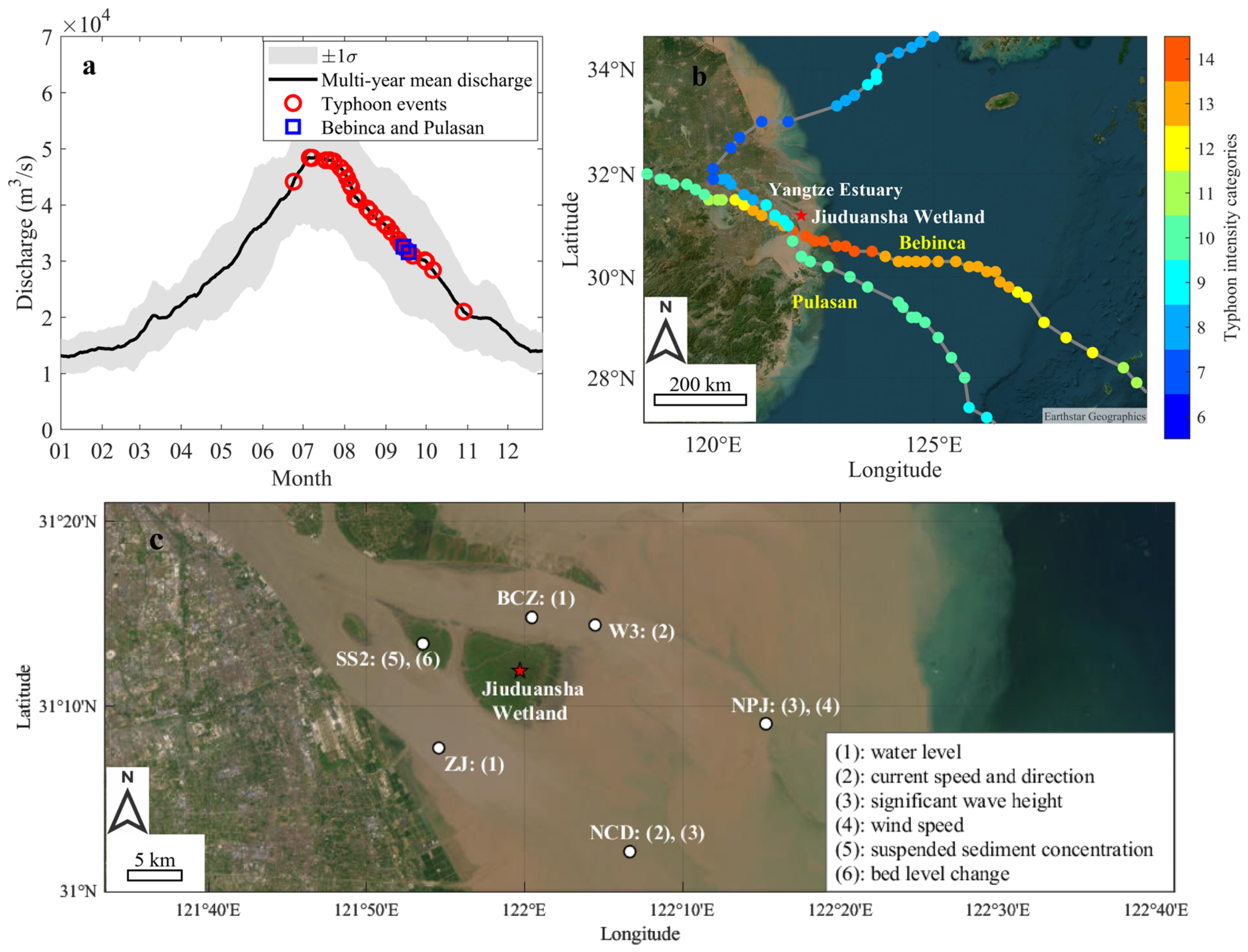
This study focused on two consecutive typhoons, Bebinca and Pulasan, which affected the Yangtze Estuary from 14 to 22 September 2024. As shown in Figure 1a, these events occurred during the recession stage of the Yangtze River flood season. The discharge at Datong Station during the 2024 typhoon period ranged from approximately 18,500 to 20,300 m³/s and remained within the ±1σ range of the multi-year mean discharge. This indicates a relatively typical late-flood-season runoff condition rather than an extreme river-discharge event.

Figure 1b shows the tracks and intensity categories of Bebinca and Pulasan. Both typhoons passed close to the Yangtze Estuary and the Jiuduansha Wetland. As Bebinca approached the estuary, its intensity increased and reached category 14 near the Shanghai region, corresponding to a maximum wind speed of approximately 41.5–46.1 m/s. Pulasan also intensified when passing near the estuary, reaching category 10, corresponding to approximately 24.5–28.4 m/s. These two consecutive events therefore provided a suitable case for examining tidal-flat response under compound typhoon forcing.

In the emulator framework, Bebinca was used for model training, while Pulasan was used for independent validation. This design allowed the emulator to be evaluated under a different typhoon event rather than only under the same forcing condition.

2.2. Field Observations

Multi-source field observations were used to support forcing analysis and model validation around the Jiuduansha Wetland study area (Figure 1c). The hydrodynamic, wave, wind, and suspended sediment observations were provided by the Shanghai Estuarine and Coastal Science Research Center and were available at an hourly resolution during the typhoon period from 14 to 22 September 2024. Water level was measured at BCZ and ZJ, current speed and direction at W3 and NCD, significant wave height at NPJ and NCD, wind speed at NPJ, and SSC at SS2. Bed-level change at SS2 was measured before and after the typhoon period using an RTK-GNSS system, with nominal accuracies of approximately 8 mm horizontally and 15 mm vertically. Harmonic analysis was applied to the observed water level to separate astronomical tide and storm-surge components. Rainfall data and atmospheric fields were obtained from the hourly ERA5 reanalysis product (https://cds.climate.copernicus.eu/datasets (accessed on 5 June 2025)), with a spatial resolution of 0.25° × 0.25°. Wang et al. [5] reported that ERA5 wind speed tends to underestimate typhoon-period wind intensity in the Yangtze Estuary and applied a correction coefficient of 1.4. In this study, ERA5 wind speed at the nearest grid cell was compared with the observed wind speed at the NPJ station, and a uniform correction coefficient of 1.5 was applied to ERA5 wind speed over the model domain.

Vegetation parameters were estimated from Landsat 8 imagery acquired on 11 August 2024. The enhanced vegetation index (EVI) was first calculated for the Jiuduansha Wetland. Vegetation biomass was then estimated using empirical relationships between field-measured biomass and EVI for Phragmites australis and Spartina alterniflora communities. Finally, vegetation parameters, including mean stem diameter, mean plant height, and plant density, were derived from fitted relationships between biomass and these vegetation properties. Details of these relationships are provided in the Supplementary Materials. These observational, reanalysis, and vegetation data were used to characterize the compound hydrodynamic response, validate the coupled numerical model, and provide vegetation parameters before generating emulator training and validation samples.

2.3. Numerical Model

A coupled MIKE21 FM model was established to simulate hydrodynamics, waves, suspended sediment transport, and bed evolution during the typhoon period [15]. The model was used not only to reproduce the observed typhoon-period processes but also to generate physically consistent hydrodynamic and morphodynamic samples for emulator training and testing. The coupled modelling system included hydrodynamic, spectral wave, sediment transport, and morphodynamic modules.

The hydrodynamic module was based on the depth-integrated shallow water equations. The continuity equation can be written as

$${\displaystyle \frac{\mathsf{\partial }\eta }{\mathsf{\partial }t}}+{\displaystyle \frac{\mathsf{\partial }\left(hu\right)}{\mathsf{\partial }x}}+{\displaystyle \frac{\mathsf{\partial }\left(hv\right)}{\mathsf{\partial }y}}=R$$

(1)

where $\eta$ is the free-surface elevation, $h$ is the total water depth, $u$ and $v$ are depth-averaged velocities in the $x$ and $y$ directions, $t$ is time, and $R$ is rainfall intensity. The corresponding depth- inteqrated momentum equations are expressed as

$${\displaystyle \frac{\mathsf{\partial }\left(hu\right)}{\mathsf{\partial }t}}+{\displaystyle \frac{\mathsf{\partial }\left(h{u}^2\right)}{\mathsf{\partial }x}}+{\displaystyle \frac{\mathsf{\partial }\left(huv\right)}{\mathsf{\partial }y}}=-fhv-gh{\displaystyle \frac{\mathsf{\partial }\eta }{\mathsf{\partial }x}}+{\displaystyle \frac{{\tau }_{sx}-{\tau }_{bx}}{\rho }}+{\displaystyle \frac{1}{\rho }}\left({\displaystyle \frac{\mathsf{\partial }{S}_{xx}}{\mathsf{\partial }x}}+{\displaystyle \frac{\mathsf{\partial }{S}_{xy}}{\mathsf{\partial }y}}\right)+D_x$$

(2)

$${\displaystyle \frac{\mathsf{\partial }\left(hv\right)}{\mathsf{\partial }t}}+{\displaystyle \frac{\mathsf{\partial }\left(huv\right)}{\mathsf{\partial }x}}+{\displaystyle \frac{\mathsf{\partial }\left(h{v}^2\right)}{\mathsf{\partial }y}}=fhu-gh{\displaystyle \frac{\mathsf{\partial }\eta }{\mathsf{\partial }y}}+{\displaystyle \frac{{\tau }_{sy}-{\tau }_{by}}{\rho }}+{\displaystyle \frac{1}{\rho }}\left({\displaystyle \frac{\mathsf{\partial }{S}_{xy}}{\mathsf{\partial }x}}+{\displaystyle \frac{\mathsf{\partial }{S}_{yy}}{\mathsf{\partial }y}}\right)+D_y$$

(3)

where $g$ is gravitational acceleration, $f$ is the Coriolis parameter, $\rho$ is water density, ${\tau }_{sx}$ and ${\tau }_{sy}$ are surface shear stresses, ${\tau }_{bx}$ and ${\tau }_{by}$ are bottom shear stresses, $S_{xx},S_{xy}$, and $S_{yy}$ are wave radiation stress components, and $D_x$ and $D_y$ represent horizontal diffusion and residual terms.

The spectral wave module solved the wave action balance equation,

$${\displaystyle \frac{\mathsf{\partial }N}{\mathsf{\partial }t}}+{\displaystyle \frac{\mathsf{\partial }\left(c_{x}N\right)}{\mathsf{\partial }x}}+{\displaystyle \frac{\mathsf{\partial }\left(c_{y}N\right)}{\mathsf{\partial }y}}+{\displaystyle \frac{\mathsf{\partial }\left(c_{\sigma }N\right)}{\mathsf{\partial }\sigma }}+{\displaystyle \frac{\mathsf{\partial }\left(c_{\theta }N\right)}{\mathsf{\partial }\theta }}={\displaystyle \frac{S}{\sigma }}$$

(4)

where $N$ is wave action density, $\sigma$ is relative angular frequency, $\theta$ is wave direction, $c_x,c_{y\prime },c_{\sigma }$, and $c_{\theta }$ are propagation velocities in physical, frequency, and directional spaces, and $S$ is the total source term. The total source term includes wind input, nonlinear wave interaction, whitecapping dissipation, bottom-friction dissipation, and depth-induced breaking.

$$S=S_{in}+S_{nl}+S_{ds}+S_{bot}+S_{surf}$$

(5)

Suspended sediment transport was described using a depth-averaged advection–diffusion equation,

$${\displaystyle \frac{\mathsf{\partial }\left(h\bar{c}\right)}{\mathsf{\partial }t}}+{\displaystyle \frac{\mathsf{\partial }\left(hu\bar{c}\right)}{\mathsf{\partial }x}}+{\displaystyle \frac{\mathsf{\partial }\left(hv\bar{c}\right)}{\mathsf{\partial }y}}={\displaystyle \frac{\mathsf{\partial }}{\mathsf{\partial }x}}\left(h{D}_x{\displaystyle \frac{\mathsf{\partial }\bar{c}}{\mathsf{\partial }x}}\right)+{\displaystyle \frac{\mathsf{\partial }}{\mathsf{\partial }y}}\left(h{D}_y{\displaystyle \frac{\mathsf{\partial }\bar{c}}{\mathsf{\partial }y}}\right)+S_{sed}$$

(6)

where $\bar{c}$ is depth-averaged suspended sediment concentration, $D_x$ and $D_y$ are horizontal diffusion coefficients, and $S_{sed}$ is the net sediment source term. The erosion and deposition fluxes were calculated using the Krone-Partheniades formulations,

$$S_d=w_s{c}_b\left(1-{\displaystyle \frac{{\tau }_b}{{\tau }_{cr,d}}}\right), {\tau }_b<{\tau }_{cr,d}$$

(7)

$$S_e=E\left({\displaystyle \frac{{\tau }_b}{{\tau }_{cr,e}}}-1\right), {\tau }_b>{\tau }_{cr,e}$$

(8)

where $S_d$ is the deposition flux, $S_c$ is the erosion flux, $w_s$ is settling velocity, $c_b$ is near-bed suspended sediment concentration, $E$ is erosion rate, ${\tau }_b$ is bottom shear stress, and ${\tau }_{cr,d}$ and ${\tau }_{cr,e}$ are critical shear stresses for deposition and erosion. Bed evolution was computed from the net sediment flux,

$$\left(1-{\epsilon }_p\right){\rho }_s{\displaystyle \frac{\mathsf{\partial }{z}_b}{\mathsf{\partial }t}}=S_d-S_e$$

(9)

where ${\epsilon }_p$ is bed porosity, ${\rho }_s$ is sediment density, and $z_b$ is bed elevation.

Vegetation effects on flow were represented by introducing a vegetation drag term ${\mathrm{F}}_v$ into the depth-integrated momentum equations. In addition, following Suzuki et al. [32], vegetation-induced wave-energy dissipation was represented in the wave spectrum equation by the energy dissipation term $S_{\mathrm{v}\mathrm{e}\mathrm{g}}\left(f,\theta \right)$. The corresponding mathematical formulations are:

$${\mathrm{F}}_v={\displaystyle \frac{1}{2}}{C}_D{d}_s{N}_v{h}_v^{\ast }{u}_v\left|u_v\right|$$

(10)

$$S_{\mathrm{v}\mathrm{e}\mathrm{g}}\left(f,\theta \right)=-\sqrt{{\displaystyle \frac{2}{\pi }}}g{C}_D{d}_s{N}_v{\left({\displaystyle \frac{\bar{k}}{2\pi \bar{f}}}\right)}^3{\displaystyle \frac{{\mathrm{s}\mathrm{i}\mathrm{n}\mathrm{h}}^3\left(k{h}_v^{\ast }\right)+3\mathrm{s}\mathrm{i}\mathrm{n}\mathrm{h}\left(k{h}_v^{\ast }\right)k{h}_v}{3k{\mathrm{c}\mathrm{o}\mathrm{s}}^3\left(kh\right)}}\sqrt{E_{\mathrm{tot}}E\left(f,\theta \right)}$$

(11)

where $C_D$ is the drag coefficient (dimensionless); $d_s$ is the stem diameter $\left(\mathrm{m}\right); h_v^{\ast }=\mathrm{m}\mathrm{i}\mathrm{n}\left(h_v,h\right)$ is the effective vegetation height (the smaller of vegetation height and water depth) (m); $N_v$ is the vegetation density (number per unit area) (stems m⁻²); $u_v$ is the apparent velocity vector (m/s), which denotes the effective velocity acting on vegetation stems; $\left|u_v\right|$ is its magnitude (m/s); $\bar{k}$ is the mean wave number (m⁻¹) $\bar{f}$ is the mean frequency (Hz); $E_{\mathrm{t}\mathrm{o}\mathrm{t}}$ is the total wave energy (m²/Hz/rad); and $E\left(f,\theta \right)$ is the wave energy density corresponding to frequency $f$ and propagation direction $\theta .$

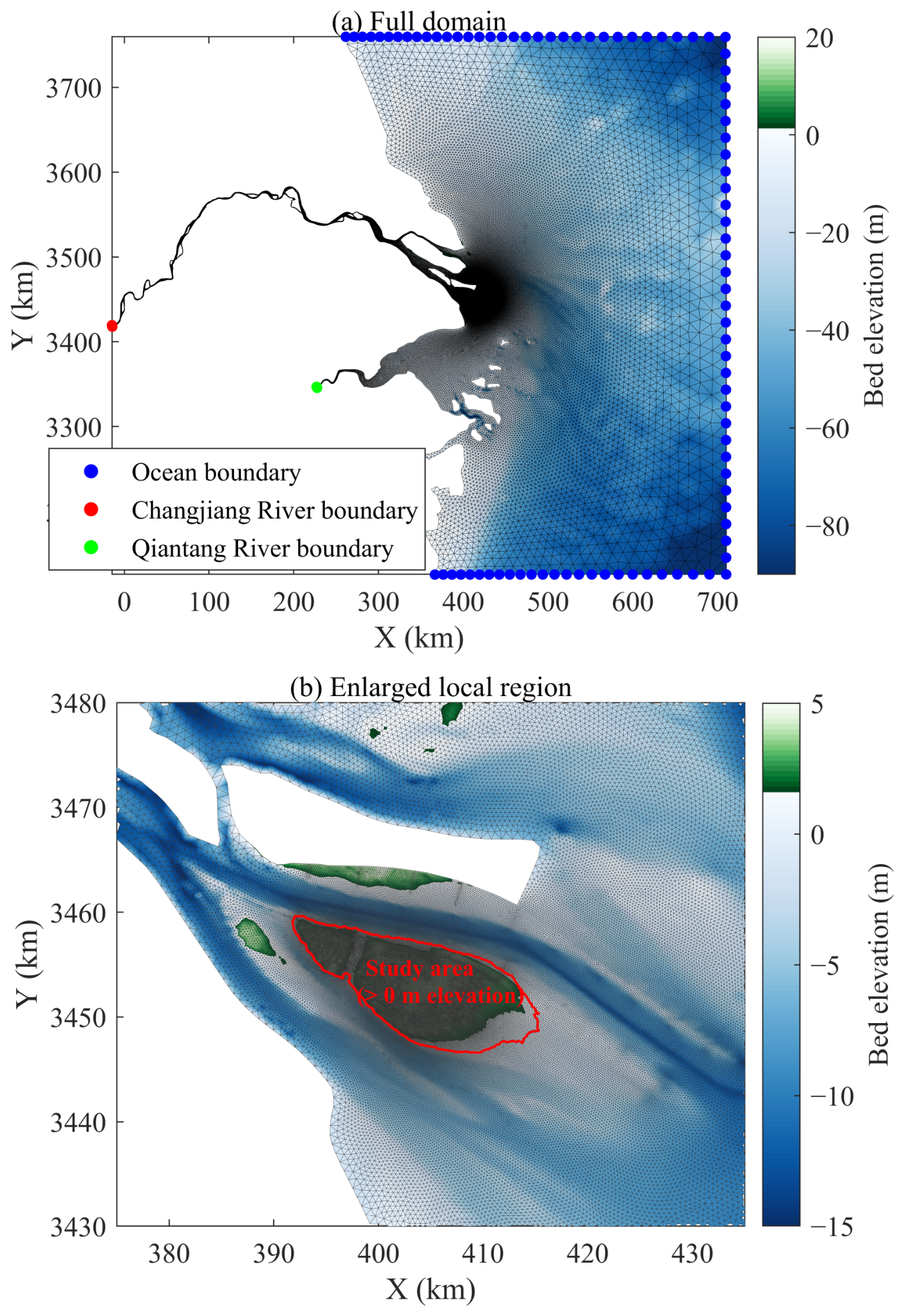
The model domain covers the lower Yangtze River from Datong Station, the Yangtze Estuary, Hangzhou Bay, and the adjacent offshore waters. It extends approximately 700 km in both the east–west and north–south directions (Figure 2a). Three open boundaries were specified, including the offshore boundary, the Yangtze River boundary, and the Qiantang River boundary. This large-scale domain covers the main region affected by the typhoons and captures the regional hydrodynamic processes during the study period. The computational grid consists of unstructured triangular elements, with 112,491 nodes and 220,710 elements. The red outline in Figure 2b indicates the Jiuduansha Wetland study area above the 0 m elevation contour, which was used for morphodynamic analysis and emulator prediction. This area was locally refined with a minimum mesh size of approximately 30 m. Bathymetric data were obtained from the 2022 Yangtze Estuary survey. Manning’s roughness coefficient was calibrated for different water-depth zones to improve tidal propagation and tidal-range simulation, with calibrated values ranging from 68 to 94 m^1/3/s [5]. The simulation period was from 14 to 22 September 2024, with a model time step of 180 s.

The offshore boundary was forced using eight major tidal constituents from the TPXO8 model (https://www.tpxo.net/), including M2, S2, N2, K2, K1, P1, O1, and Q1. The offshore SSC was set to 0.01 kg/m³ because suspended sediment concentration is relatively low near the offshore boundary [33]. The Yangtze River boundary used observed discharge and SSC from Datong Station. The Qiantang River boundary was assigned a constant discharge of 925 m³/s and an SSC of 0.1 kg/m³ [33]. Horizontal eddy viscosity was calculated using the Smagorinsky formulation with a constant coefficient of 0.28. The horizontal sediment diffusivity was specified using the scaled eddy viscosity formulation, with a constant scaling factor of 0.8. The main sediment transport parameters are listed in

Table 1. Main sediment parameters used in the MIKE21 FM model.

Parameter	Symbol	Value
Settling velocity	ws	0.3 mm/s
Sediment density	ρs	2650 kg/m3
Dry bed density	ρd	800 kg/m3
Critical erosion shear stress	τcr,e	0.5 N/m2
Critical deposition shear stress	τcr,d	0.3 N/m2
Erosion rate	E	2.5 × 10−5 kg/m2/s

were selected based on previous Yangtze Estuary hydrodynamic and sediment transport modelling studies by Zhao et al. [33]. The critical erosion shear stress and erosion rate were further adjusted according to the observed SSC and event-scale bed-level change. The corrected ERA5 wind and pressure fields were used as atmospheric forcing for the wave and hydrodynamic simulations. The wave-module parameters followed Wang et al. [5]. The breaking parameter was set to 0.8, the bottom-friction grain size d50 was set to 0.00025 m, and the wave dissipation coefficient was set to 0.15. Following Zuo et al. [34], the vegetation drag coefficient $C_D$ was set to 1.0.

2.4. Emulator Inputs, Dataset, and Architecture

Physically meaningful input variables for the emulator were selected based on the main drivers of tidal-flat erosion and deposition during typhoon events. Bed-level change is directly controlled by wave–current-induced sediment transport and bottom shear stress (BSS). In the coupled numerical model, vegetation effects were represented through vegetation-induced flow resistance and wave-energy dissipation; therefore, their influence was already reflected in the simulated hydrodynamic and shear-stress fields. Rainfall mainly affects local microtopography, such as tidal channels, and has limited influence on large-scale tidal-flat morphodynamics [35]; therefore, it was not included as a direct emulator input. Tides and river discharge were considered as background controls for hydrodynamics and sediment supply. Based on this understanding, generalized Lagrangian mean velocity (GLMV) and BSS were chosen as emulator inputs. GLMV combines the Eulerian depth-averaged velocity $\left(U_E\right)$ and the Stokes drift velocity $\left(U_S\right)$:

$$U_{GLM}=U_E+U_S$$

(12)

and its magnitude is calculated as

$$U_{GLM}=\sqrt{u_{GLM}^2+v_{GLM}^2}$$

(13)

Bottom shear stress is expressed conceptually as

$${\tau }_b=\rho C_f\left|u\right|u$$

(14)

where $\rho$ is water density, $C_f$ is the bed-friction coefficient, and u is the depth-averaged velocity. In the emulator, BSS represents local erosion-deposition potential, while GLMV represents the combined transport effect of currents and wave-induced drift.

The prediction target is the current-timestep bed-level change (CTBLC):

$$\Delta z_b^t=z_b^t-z_b^{t-1}$$

(15)

and cumulative bed-level change is reconstructed as

$$\Delta Z_b^T={\displaystyle \sum _{t=1}^T}\Delta z_b^t$$

(16)

Data were extracted from the Jiuduansha analysis region and cropped to $552\times 868$ pixels, then interpolated to a spatial resolution of 30 m. All variables were normalized using min-max scaling.

$$X^{\ast }={\displaystyle \frac{X-X_{\mathrm{m}\mathrm{i}\mathrm{n}}}{X_{\mathrm{m}\mathrm{a}\mathrm{x}}-X_{\mathrm{m}\mathrm{i}\mathrm{n}}}}$$

(17)

Typhoon Bebinca was used to construct the training dataset, while Typhoon Pulasan was used as an independent validation event. To expand the range of hydrodynamic conditions represented in the training data, additional numerical scenarios were generated by perturbing wind-pressure forcing, Yangtze River discharge, and tidal range. These scenarios should be interpreted as prescribed hydrodynamic perturbation experiments rather than independent typhoon events. Each numerical scenario produced 1920 time-step samples. The original training dataset from the Bebinca-based scenarios contained 30,720 image samples. To reduce data redundancy and computational cost, the samples were temporally downsampled at an interval of five time steps, resulting in 6144 training samples. The Pulasan-based validation scenarios were not downsampled and were evaluated chronologically to reconstruct cumulative bed-level change. The scenario settings are summarized in

Table 2. Training and validation scenarios under prescribed hydrodynamic perturbations.

Dataset	Case	Wind-Pressure Factor	Yangtze Discharge	Tide Condition
Training, Bebinca	C1	1.0	20,000 m3/s	Moderate tide
Training, Bebinca	C2	0.8	20,000 m3/s	Moderate tide
Training, Bebinca	C3	0.6	20,000 m3/s	Moderate tide
Training, Bebinca	C4	0.4	20,000 m3/s	Moderate tide
Training, Bebinca	C5	1.0	40,000 m3/s	Moderate tide
Training, Bebinca	C6	1.0	60,000 m3/s	Moderate tide
Training, Bebinca	C7	1.0	20,000 m3/s	Neap tide
Training, Bebinca	C8	1.0	20,000 m3/s	Spring tide
Validation, Pulasan	C9	1.0	20,000 m3/s	Spring tide
Validation, Pulasan	C10	1.0	20,000 m3/s	Neap tide
Validation, Pulasan	C11	1.0	60,000 m3/s	Spring tide
Validation, Pulasan	C12	0.4	20,000 m3/s	Spring tide

Note: The wind-pressure factor denotes the scaling coefficient applied to the corrected ERA5 typhoon wind-pressure forcing. A value of 1.0 represents the original corrected forcing, whereas values of 0.8, 0.6, and 0.4 represent prescribed reductions in typhoon forcing intensity. Tide conditions were classified from a representative spring–neap tidal cycle in September 2024. Spring, moderate, and neap tides indicate different tidal stages within this cycle rather than fixed tidal ranges.

. In the perturbation-based evaluation, wave forcing was represented by comparing C9 and C12, tidal forcing by comparing C9 and C10, and runoff forcing by comparing C11 and C9. These controlled case comparisons allowed the effects of different hydrodynamic perturbations on predicted bed-level change to be evaluated.

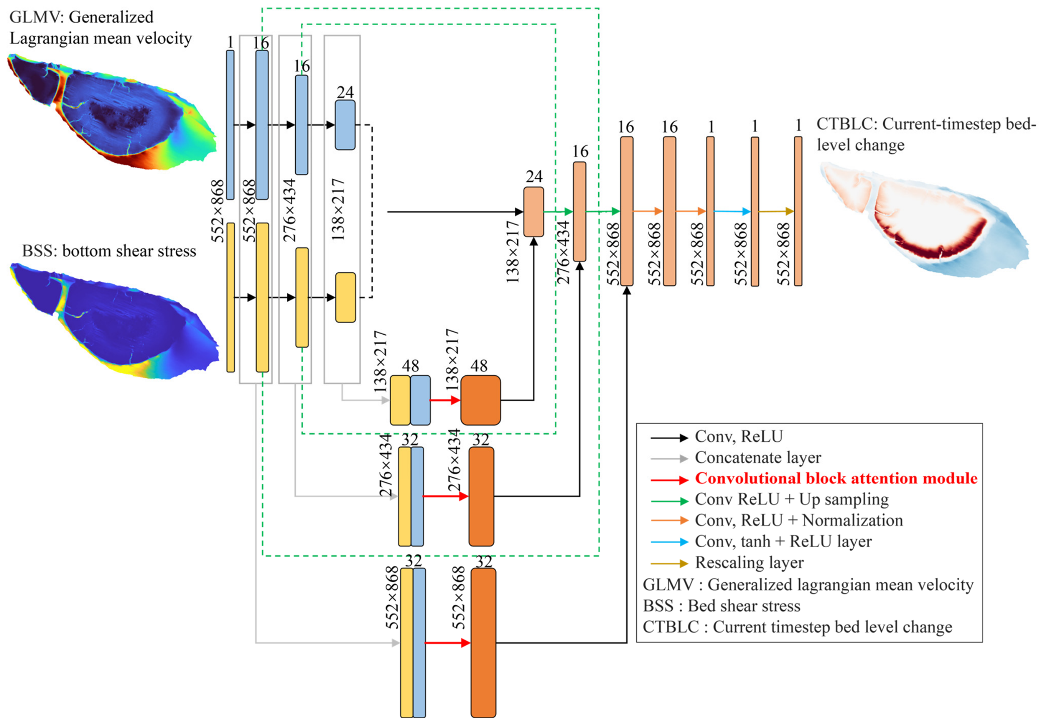
The emulator was implemented in PyTorch 2.6.0 using a UNet encoder–decoder architecture, which is suitable for spatial prediction because it extracts multiscale features and preserves local details through skip connections [36]. To better capture spatially heterogeneous erosion–deposition patterns, a Convolutional Block Attention Module (CBAM) was introduced into the UNet framework, forming the CBAM-UNet used in this study (Figure 3). The model takes two-channel input fields, including GLMV and BSS, and predicts the single-channel bed-level increment at the current time step. All input and output fields were resized to 868 × 552 pixels before training. The encoder contains three feature levels with 16, 16, and 24 channels, respectively. Two stride-2 convolutional layers are used for downsampling, producing a deepest feature map with one quarter of the original spatial resolution. Most convolutional layers use 3 × 3 kernels with ReLU activation, and selected blocks use dilated convolutions with a dilation rate of 3 to enlarge the receptive field. The decoder reconstructs the bed-level increment field using transposed convolutions and skip connections. CBAM was inserted after each encoder convolutional block and sequentially applies channel and spatial attention [37]. Channel attention enhances informative hydrodynamic and shear-stress-related feature maps, whereas spatial attention emphasizes morphodynamically sensitive regions, such as bare-flat edges and marsh margins.

For an intermediate feature map $F$, the CBAM operation is defined as

$$F^{\prime }=M_c\left(F\right)\otimes F, F^{″}=M_s\left(F^{\prime }\right)\otimes F^{\prime }$$

(18)

where $M_c$ and $M_s$ denote channel and spatial attention maps, respectively, and $\otimes$ indicates element-wise multiplication. Channel attention is obtained from global average and max pooling:

$$M_c\left(F\right)=\sigma \left[\begin{array}{c}MLP\left(AvgPool\left(F\right)\right)+MLP\left(MaxPool\left(F\right)\right)\end{array}\right]$$

(19)

and spatial attention is computed as

$$M_s\left(F\right)=\sigma \left[f^{k\times k}\left(\left[AvgPool\left(F\right);MaxPool\left(F\right)\right]\right)\right]$$

(20)

where $f^{k\times k}$ denotes a convolution operation and [;] denotes feature concatenation. Finally, the emulator can be represented as

$$\widehat{\Delta z_b^t}=F_{\theta }\left({\mathbf{U}}_{GLMV}^t,{\mathsf{\tau }}_{BSS}^t\right)$$

(21)

where $F_{\theta }$ is the CBAM-UNet with trainable parameters $\theta$, and $\widehat{\Delta z_b^t}$ is the predicted bed-level increment at time $t.$

2.5. Training Strategy and Evaluation Metrics

The model was trained using the RMSprop optimizer with an initial learning rate of 0.005. The maximum number of training epochs was 200. Early stopping was used to reduce overfitting, and training was stopped if validation performance did not improve for 15 consecutive epochs. Training was conducted on a personal computer equipped with an Intel Core i7-10700K CPU, 64 GB memory (Intel Corporation, Santa Clara, CA, USA), and an NVIDIA RTX 2070 SUPER GPU (Nvidia Corporation, Santa Clara, CA, USA). CUDA Toolkit 12.7 was used for GPU acceleration.

The loss function included both current-timestep error and cumulative bed-level error. This design allowed the model to learn both local bed-level increments and cumulative morphodynamic evolution. The current-timestep loss was defined as

$$L_{step}={\displaystyle \frac{1}{N}}{\displaystyle \sum _{i=1}^N}{\left(\widehat{\Delta z_{b,i}^t}-\Delta z_{b,i}^t\right)}^2$$

(22)

where $N$ is the number of spatial pixels.

The cumulative loss was defined as

$$L_{cum}={\displaystyle \frac{1}{N}}{\displaystyle \sum _{i=1}^N}{\left({\displaystyle \sum _{t=1}^T}\widehat{\Delta z_{b,i}^t}-{\displaystyle \sum _{t=1}^T}\Delta z_{b,i}^t\right)}^2$$

(23)

The total loss was calculated as

$$L={\lambda }_1{L}_{step}+{\lambda }_2{L}_{cum}, {\lambda }_1={\lambda }_2=0.5$$

(24)

Model validation for the numerical model was evaluated using RMSE and Skill. RMSE was calculated as

$$RMSE=\sqrt{{\displaystyle \frac{1}{N}}{\displaystyle \sum _{i=1}^N}{\left(M_i-D_i\right)}^2}$$

(25)

where $M_i$ and $D_i$ are simulated and observed values. Skill was calculated as

$$Skill=1-{\displaystyle \frac{{\displaystyle {\sum }_{i=1}^N}{\left(M_i-D_i\right)}^2}{{\displaystyle {\sum }_{i=1}^N}{\left(\left|M_i-\bar{D}\right|+\left|D_i-\bar{D}\right|\right)}^2}}$$

(26)

where $\bar{D}$ is the mean observed value.

Emulator prediction accuracy was evaluated using cumulative $RMSE$,

$$RMS{E}_{cum}^T=\sqrt{{\displaystyle \frac{1}{N}}{\displaystyle \sum _{i=1}^N}{\left(\widehat{\Delta Z_{b,i}^T}-\Delta Z_{b,i}^T\right)}^2}$$

(27)

Computational efficiency was evaluated across all validation cases. The runtime of the full MIKE21 FM simulation with spectral wave, hydrodynamic, and morphodynamic modules was compared with that of the workflow using only spectral wave and hydrodynamic modules plus the trained emulator. The runtime reduction rate was calculated as

$$R_{time}={\displaystyle \frac{T_{full}-\left(T_{SW+HD}+T_{DL}\right)}{T_{full}}}\times 100\mathrm{\%}$$

(28)

where $T_{full}$ is the runtime of the full SW + HD + MT model, $T_{SW+HD}$ is the runtime of the spectral wave and hydrodynamic modules, and $T_{DL}$ is the prediction time of the deep learning emulator.

3. Results

3.1. Observed Typhoon Response and Numerical Model Validation

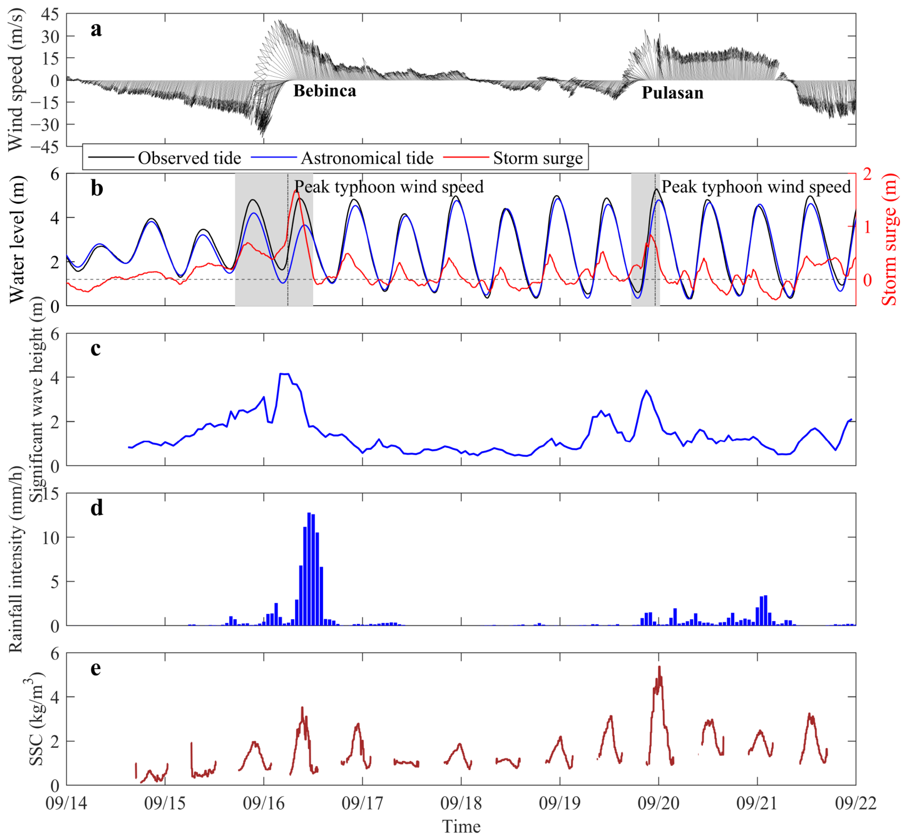
The two successive typhoon events produced distinct but related hydrodynamic and sediment responses over the tidal flat (Figure 4). During the early stage of Typhoon Bebinca from 14 to 15 September 2024, wind speed increased from 4.21 m/s to 15.51 m/s, storm surge reached 0.71 m, and significant wave height increased from 0.81 m to 2.59 m. Rainfall intensity remained relatively low, below 2.52 mm/h, while suspended sediment concentration increased from 0.58 kg/m³ to 1.96 kg/m³. These changes indicate that the increasing wind-wave forcing enhanced sediment resuspension during the early stage of Bebinca.

As Bebinca made landfall, the hydrodynamic forcing intensified further. Wind speed reached a peak value of 39.2 m/s, storm surge increased to 1.71 m, and significant wave height reached 4.15 m. Rainfall intensity also increased to 12.79 mm/h, while suspended sediment concentration rose to 3.52 kg/m³. These observations suggest that strong wave action, elevated water level, and storm-induced bed shear stress jointly promoted sediment resuspension during the peak stage of Bebinca. Around 24:00 on 16 September, as the typhoon moved inland, wind speed decreased to 8.35 m/s, and the other hydrodynamic variables gradually returned to near pre-typhoon levels.

Typhoon Pulasan was weaker than Bebinca, but it showed a similar overall hydrodynamic response pattern. The maximum wind speed during Pulasan was 25.38 m/s, the peak storm surge was 0.85 m, and the maximum significant wave height reached 3.41 m. Rainfall intensity was only 1.36 mm/h. However, suspended sediment concentration increased markedly and reached a maximum value of 5.38 kg/m³, exceeding that observed during Bebinca. This high concentration was likely associated with the overlap between Pulasan and spring tide, which enhanced tidal resuspension and sediment transport.

Overall, the observations show that typhoon-period tidal-flat sediment dynamics cannot be explained by wind intensity or wave forcing alone. Instead, wind waves, storm surge, astronomical tide, rainfall, runoff, and sediment availability jointly shaped the compound hydrodynamic conditions during the two events. As shown in Figure 4, Bebinca mainly reflected the effect of strong wind-wave forcing, whereas Pulasan highlighted the important role of tidal phase in regulating suspended sediment response. This contrast provides a useful basis for evaluating whether the numerical model and emulator can reproduce tidal-flat morphodynamic change under different compound forcing conditions.

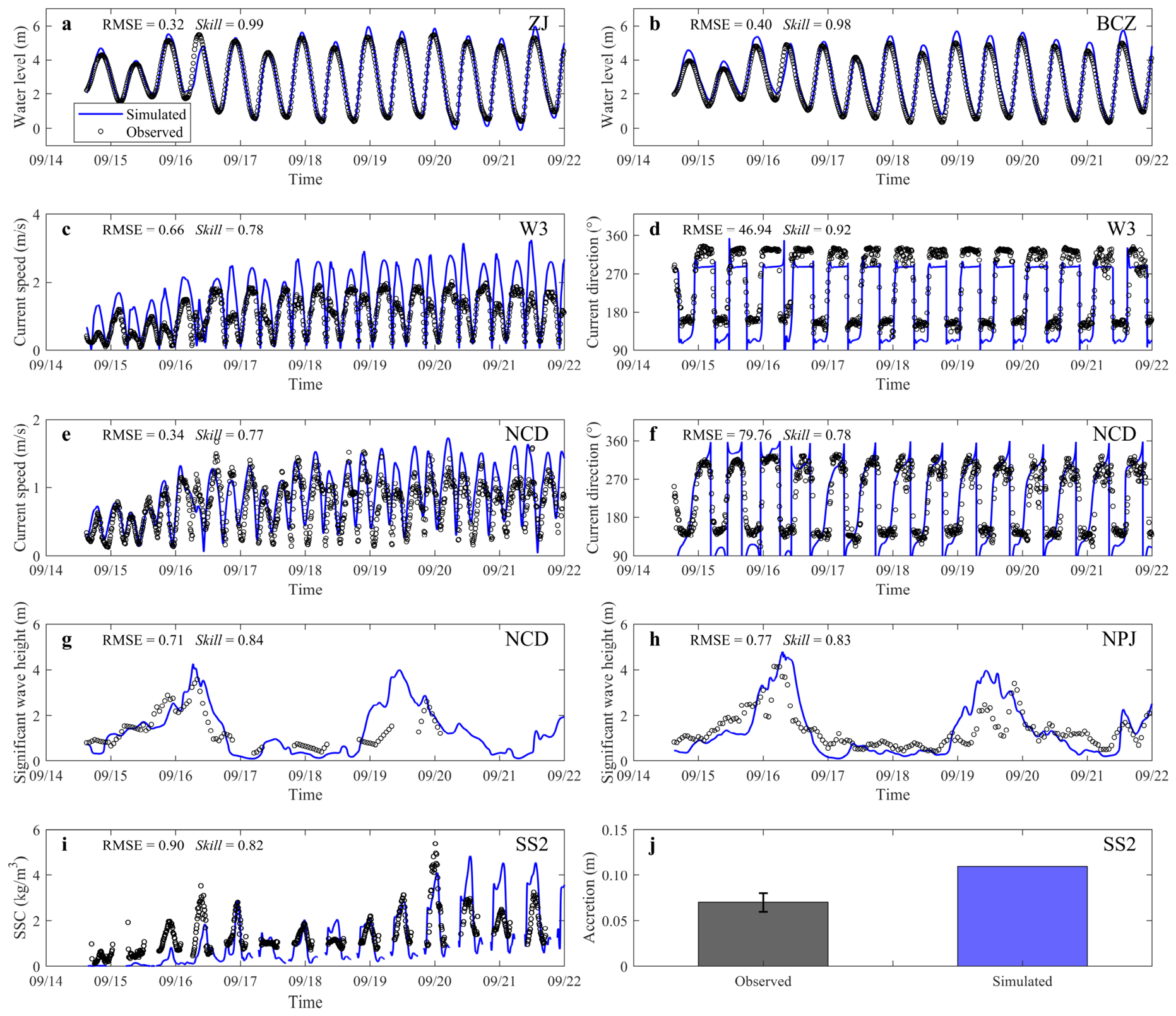
The MIKE21 FM model reproduced the main hydrodynamic and sediment transport processes during the typhoon period (Figure 5). The model showed the best performance for water level, with RMSE values of 0.32–0.40 m and Skill values of 0.98–0.99, indicating that the large-scale tidal propagation and storm-surge response were well captured. Velocity simulations showed moderate accuracy, with RMSE values of 0.34–0.66 m/s and Skill values of 0.77–0.78. Flow-direction errors were larger, with RMSE values ranging from 46.94° to 79.76°, but the corresponding Skill values remained between 0.78 and 0.92. These larger directional errors may be related to tidal flow reversal, local shallow-flat effects, and the sensitivity of flow direction during low-velocity periods, when small velocity-vector errors can lead to large angular deviations.

Wave and suspended sediment simulations also agreed reasonably well with observations. Significant wave-height RMSE ranged from 0.71 m to 0.77 m, with Skill values of 0.83–0.84. The remaining wave-height errors may partly reflect uncertainties in typhoon wind forcing, local wave growth, and depth-limited wave transformation over shallow tidal flats. SSC at SS2 had an RMSE of 0.90 kg/m³ and a Skill value of 0.82, indicating that the model captured the main temporal variability in suspended sediment concentration during the event. The simulated bed-level change at SS2 was approximately 0.1 m, with an error of about 0.04 m compared with the RTK measurement. Overall, the coupled MIKE21 FM model provided a credible physical basis for generating training and validation samples for the morphodynamic emulator.

3.2. Emulator Prediction of Spatial and Temporal Bed-Level Change

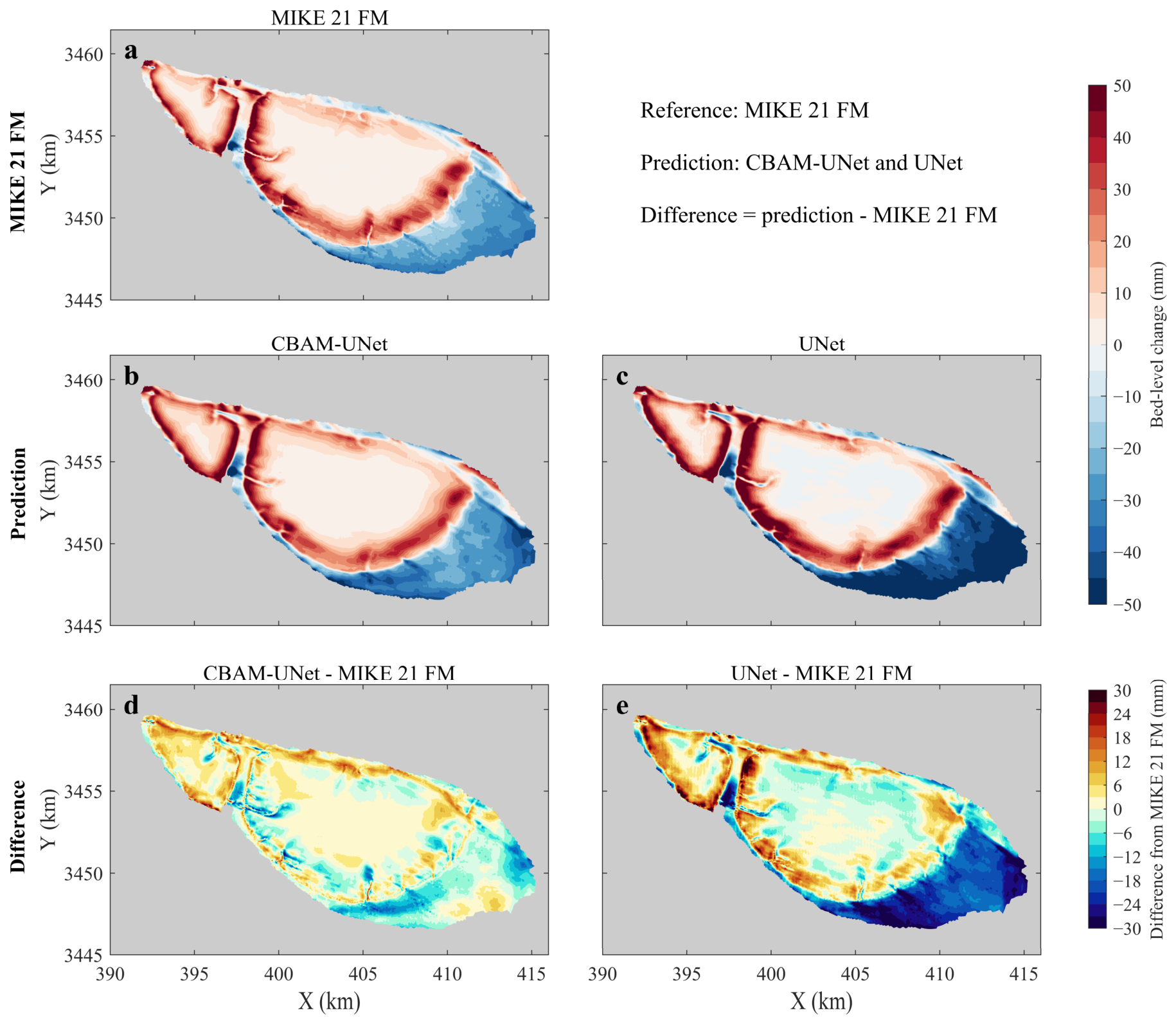
As shown in Figure S2, the study area can be broadly divided into vegetated marsh zones and non-vegetated bare-flat zones based on the EVI distribution. This zonation helps explain the spatial pattern of bed-level change in Figure 6a–c. The three models reproduced a broadly consistent erosion–deposition pattern after Typhoon Pulasan. Erosion mainly occurred over the non-vegetated bare-flat region, especially along the southeastern lower flat, where bed-level change was mostly negative and locally reached approximately −50 mm. In contrast, deposition was mainly concentrated in the vegetated marsh area and along the marsh-edge zone, where accretion was commonly on the order of several centimeters and locally greater than 50 mm. This pattern is physically reasonable because bare flats are directly exposed to wave–current forcing and are more susceptible to bed shear stress, whereas vegetation reduces flow velocity, dissipates wave energy, and promotes sediment trapping.

The error maps further highlight the differences among the models (Figure 6d–e). The conventional UNet captured the overall erosion–deposition pattern, but its prediction was more spatially smoothed and exhibited larger errors in regions with strong morphodynamic gradients. Notably, the UNet–MIKE21 FM difference map shows a pronounced negative bias over the southeastern bare-flat erosion zone, with local differences approaching −30 mm. This indicates that the conventional UNet tended to smooth sharp bed-level transitions and had limited ability to represent localized erosion intensity. By contrast, the CBAM-UNet prediction was closer to the MIKE21 FM reference result. Most errors over the central tidal flat remained relatively small, generally within approximately ±10–15 mm, with larger deviations mainly confined to the marsh edge, channel margins, and the southeastern erosion front. Compared with UNet, CBAM-UNet reduced the extent of large negative bias in the bare-flat erosion zone and better preserved the contrast between bare-flat erosion and vegetation-associated deposition.

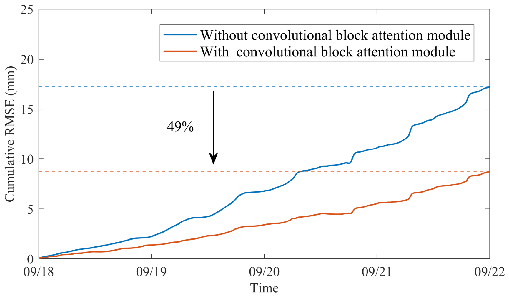
The temporal prediction results further support the spatial comparison. As shown in Figure 7, the cumulative RMSE of both models increased with time, reflecting the accumulation of single-step prediction errors during the event-scale simulation. However, the error growth rate differed substantially between the two models. The conventional UNet showed a faster increase in cumulative RMSE, especially after 20 September, and reached approximately 17.2 mm at the final time step. In contrast, CBAM-UNet maintained a slower error accumulation rate and ended with a cumulative RMSE of approximately 8.8 mm, corresponding to an error reduction of about 49%. These results indicate that the CBAM attention mechanism not only improved the spatial reconstruction of localized erosion and deposition features, but also reduced temporal error accumulation during continuous bed-level prediction. This advantage is important for event-scale tidal-flat morphodynamic emulation, where small single-step errors may accumulate into larger deviations over several tidal cycles.

3.3. Perturbation-Based Evaluation Under Different Hydrodynamic Conditions

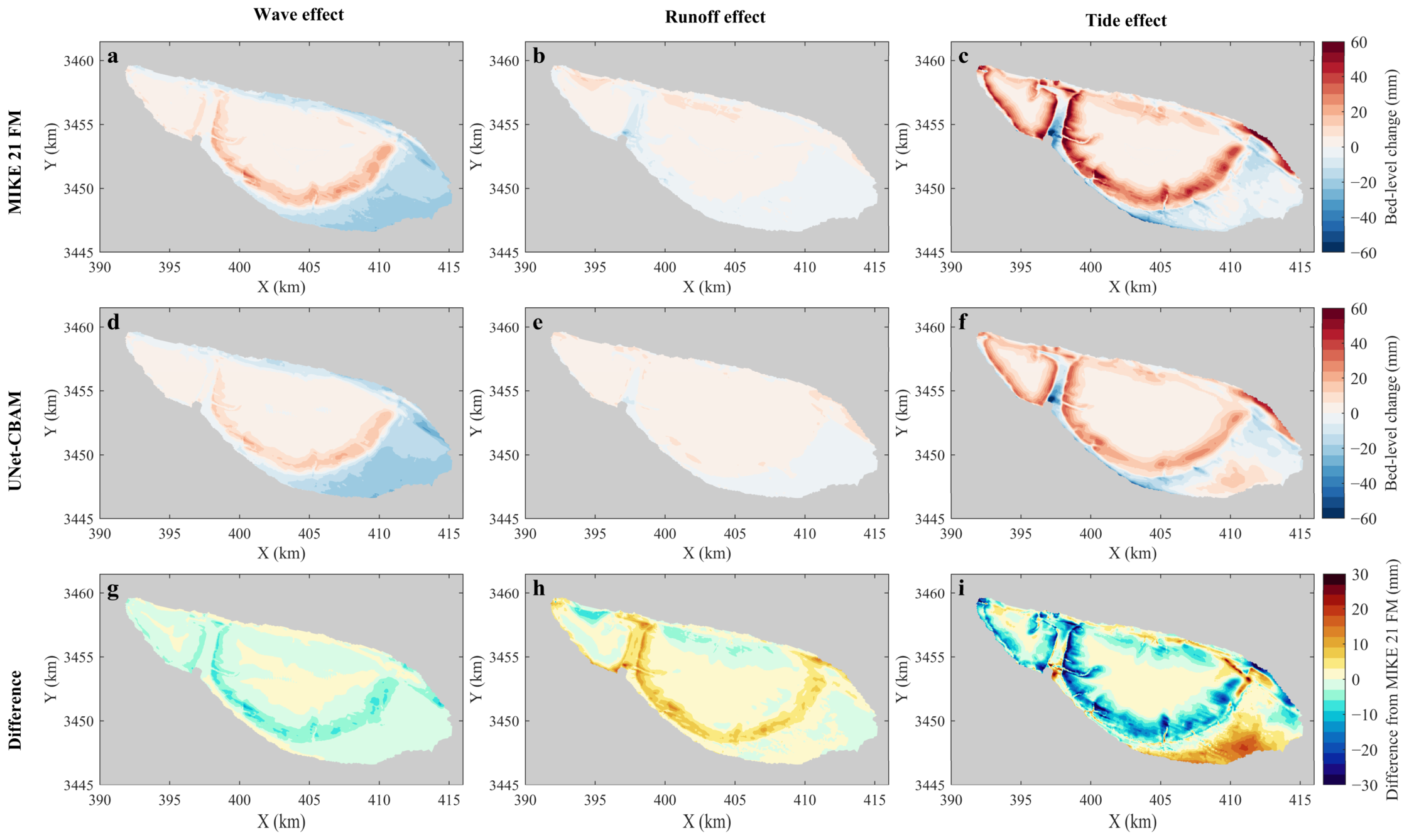
The CBAM-UNet emulator was further evaluated under prescribed wave, runoff, and tidal perturbations based on the Pulasan validation event. This experiment was designed to examine whether the emulator could respond consistently to different hydrodynamic forcing changes within the range represented by the numerical scenarios. As shown in Figure 8, the emulator reproduced the main spatial patterns of bed-level change under all three perturbation conditions, including wave forcing represented by C9–C12, tidal forcing represented by C9–C10, and runoff forcing represented by C11–C9. In the wave perturbation case, both MIKE21 FM and CBAM-UNet predicted erosion over the southeastern bare-flat region, with local bed-level decreases generally on the order of −20 to −40 mm, and deposition along the inner flat and marsh-edge zone, mostly within about 10–30 mm. The difference map indicates that most errors were relatively small, generally within ±10–15 mm, although local deviations occurred near the marsh edge and the southeastern erosion front.

The runoff perturbation produced the weakest and smoothest morphodynamic response. Both MIKE21 FM and CBAM-UNet predicted relatively small bed-level changes over most of the tidal flat, generally within ±10 mm. The difference map also shows limited errors, mainly distributed along the marsh edge and local transition zones. In contrast, the tidal perturbation generated the strongest and most spatially complex response. MIKE21 FM predicted marked deposition in the vegetated and upper-flat regions, locally exceeding 50 mm, and erosion along the lower bare flat, locally reaching approximately −40 to −60 mm. CBAM-UNet reproduced the overall erosion–deposition structure, but larger local errors occurred near channel margins, marsh-edge zones, and the southeastern lower flat, with some differences approaching ±30 mm. This indicates that tide-induced morphodynamic change is more difficult to emulate because tidal modulation affects inundation duration, flow reversal, sediment residence time, and phase-dependent sediment redistribution.

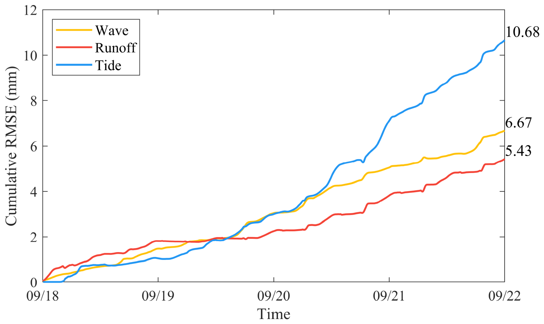
The temporal evolution of cumulative RMSE further confirms these spatial differences (Figure 9). The runoff perturbation showed the lowest final cumulative RMSE, approximately 5.43 mm, reflecting its weaker and smoother morphodynamic response. The wave perturbation had a slightly higher final cumulative RMSE of approximately 6.67 mm, whereas the tidal perturbation produced the largest error accumulation, reaching approximately 10.68 mm. The faster increase in tidal RMSE after 20 September further indicates that tidal forcing produced more complex temporal error accumulation than wave or runoff perturbations. Overall, the CBAM-UNet emulator showed consistent ability to reproduce bed-level responses under different prescribed hydrodynamic perturbations. Its performance was better under runoff and wave perturbations, where the response was relatively smooth or more directly linked to hydrodynamic forcing, while larger uncertainty occurred under tidal perturbation due to stronger tidal-phase effects, sediment redistribution, and local morphology. These results suggest preliminary cross-condition applicability within the tested forcing range.

3.4. Computational Efficiency of the Emulator Framework

The CBAM-UNet emulator showed clear computational advantages across the validation scenarios (

Table 3. Computational runtime comparison between the full SW + HD + MT model and the SW + HD + CBAM-UNet hybrid workflow for validation cases.

Case	Full SW + HD + MT Runtime (h)	SW + HD Runtime (h)	CBAM-UNet Prediction Time (s)	Runtime Reduction (%)
C9	11.81	6.89	120.00	41.38
C10	11.92	7.09	129.90	40.15
C11	12.65	7.04	122.48	44.08
C12	12.64	7.00	120.06	44.39
Average	12.25	7.01	123.11	42.50

Notes: SW, HD, and MT denote the spectral wave, hydrodynamic, and morphodynamic modules, respectively. Runtime reduction was calculated by replacing the MT module with the CBAM-UNet emulator.

). For cases C9–C12, the full process-based simulations with spectral wave, hydrodynamic, and morphodynamic modules required 11.81–12.65 h, with an average runtime of 12.25 h. In contrast, the simulations using only the spectral wave and hydrodynamic modules required 6.89–7.09 h, with an average runtime of 7.01 h. After replacing the morphodynamic module with the trained CBAM-UNet emulator, bed-level predictions were generated in only 120.00–129.90 s, with an average prediction time of 123.11 s.

This replacement substantially reduced the total computational cost. The runtime reduction ranged from 40.15% to 44.39% across the four validation cases, with an average reduction of 42.50%. The largest reduction occurred in C12, where the runtime decreased from 12.64 h to 7.00 h plus 120.06 s of emulator prediction, corresponding to a reduction of 44.39%. Even in C10, where the reduction was relatively smaller, the total runtime was still reduced by 40.15%. These results indicate that the morphodynamic module accounts for a considerable proportion of the event-scale simulation cost and that replacing it with the emulator provides stable acceleration under different validation scenarios.

The efficiency gain is particularly useful for rapid post-typhoon assessment and multi-scenario screening. Although the framework still relies on MIKE21 FM to provide hydrodynamic and wave inputs, it avoids repeatedly running the computationally expensive morphodynamic module. Therefore, the proposed framework provides a practical hybrid strategy: the process-based model maintains physically consistent hydrodynamic forcing, while the CBAM-UNet emulator accelerates bed-level prediction with acceptable accuracy. This balance between physical reliability and computational efficiency is valuable when multiple typhoon scenarios, tidal conditions, or boundary perturbations need to be evaluated.

4. Discussion

4.1. Observation-Constrained Emulation for Typhoon-Affected Tidal Flats

The results show that the observation-validated MIKE21 FM model provided a reliable physical basis for emulator training. During the two typhoons, the model reproduced the main hydrodynamic and sediment responses with acceptable accuracy, including water-level Skill values of 0.98–0.99, significant wave-height Skill values of 0.83–0.84, and suspended sediment concentration Skill of 0.82. The simulated bed-level change at SS2 differed from the RTK measurement by about 40 mm. These results indicate that the training samples were generated from a process-based model supported by event-scale observations, rather than from unconstrained numerical outputs. This is important because Bebinca and Pulasan produced different forcing combinations: Bebinca was mainly controlled by strong wind-wave forcing, whereas Pulasan had weaker wind and wave forcing but coincided with spring tide and produced higher suspended sediment concentration. Similar studies have also shown that storm-induced tidal-flat and marsh changes depend strongly on tidal phase, sediment availability, vegetation, and local morphology [1,4,7,12].

Compared with previous coastal morphodynamic emulators, the present framework is more closely linked to event-scale field evidence. Parker et al. [23] demonstrated the value of emulation for rapid estuarine modelling, while Weber De Melo et al. [28,29] showed that CNN- and UNet-based emulators can reproduce coastal or estuarine morphological evolution from numerical-model outputs. However, many existing applications mainly focus on numerical-model-driven datasets, sandy coasts, beach profiles, or generalized coastal settings. The present study extends this idea to a vegetated estuarine tidal flat affected by compound typhoon forcing. Its contribution is therefore not only the use of a neural-network emulator, but the construction of an observation-constrained emulation workflow for typhoon-period tidal-flat morphodynamics.

4.2. Contribution of CBAM Relative to Conventional UNet Emulation

The comparison between UNet and CBAM-UNet shows that the attention mechanism improved the prediction of local bed-level change. As shown in Figure 6, both models reproduced the broad erosion–deposition pattern after Pulasan, but the conventional UNet produced smoother outputs and underestimated localized high-gradient zones. This smoothing may be related to the reconstruction process of encoder–decoder networks, in which fine-scale spatial contrasts can be partly weakened during downsampling and upsampling, even though skip connections help preserve local information [36].

The improvement introduced by CBAM is reflected in both spatial pattern and temporal error accumulation. The CBAM-UNet better captured localized erosion over the bare flat and deposition near the vegetated marsh edge. The final cumulative RMSE decreased from approximately 17.2 mm for UNet to 8.8 mm for CBAM-UNet, corresponding to an error reduction of about 49% (Figure 7). From a mathematical perspective, CBAM refines convolutional features by applying adaptive multiplicative weiqhts in both the channel and spatial dimensions [37]. For an intermediate feature map $F$, channel attention first generates a channel-weight map $M_c\left(F\right)$, and the feature response is updated as $F^{\prime }=M_c\left(F\right)\otimes F$. Spatial attention then generates a spatial-weight map $M_s\left(F^{\prime }\right)$, and the refined feature becomes $F^{″}=M_s\left(F^{\prime }\right)\otimes F^{\prime }.$ Therefore, CBAM can be interpreted as a featureweighting operation in which informative channels and sensitive spatial locations receive larger weights, while less relevant responses are relatively suppressed.

This result is also consistent with the physical nature of storm-induced tidal-flat change. Previous studies have shown that storm or typhoon impacts on marshes and tidal flats are spatially heterogeneous, with erosion and deposition often concentrated around vegetation edges, tidal channels, and mudflat–marsh transition zones [1,7,38]. This mathematical mechanism is physically meaningful for tidal-flat morphodynamic emulation. The input variables, GLMV and BSS, contain spatially heterogeneous information on wave–current transport and bed shear stress. Channel attention can enhance feature maps that are more closely related to hydrodynamic and shear-stress controls, whereas spatial attention can emphasize regions where erosion–deposition gradients are concentrated, such as bare-flat edges, tidal-channel margins, marsh boundaries, and mudflat–marsh transition zones. The value of CBAM in this study is therefore not that it changes the physical mechanism of morphodynamic prediction or introduces a fundamentally new neural-network architecture. Instead, it provides an adaptive feature-refinement operation that improves the emulator’s ability to preserve local erosion–deposition gradients within an observation-supported modelling framework for muddy, vegetated estuarine tidal flats.

4.3. Computational Efficiency and Practical Implications

The perturbation results indicate that the emulator has a certain capacity to respond to different hydrodynamic forcing conditions, rather than only fitting a single validation event (Figure 8). Its better performance under runoff and wave perturbations suggests that bed-level changes driven by smoother forcing or by more direct shear-stress control are easier to emulate. In contrast, the larger error under tidal perturbation indicates that tide-modulated morphodynamics involve more complex processes, including alternating flow direction, variable inundation duration, sediment residence time, and phase-dependent redistribution. This is consistent with the observed contrast between Bebinca and Pulasan, where sediment response was not simply controlled by wind-wave intensity, but also by tidal background and sediment availability. Similar studies in the Yangtze Estuary have also shown that wave–current interaction and typhoon-induced sediment transport can substantially modify suspended sediment dynamics and bed erosion [5,11,12].

From an application perspective, the perturbation experiments are important because rapid tidal-flat assessment often requires comparison among multiple possible forcing scenarios. A process-based morphodynamic model can provide detailed physical simulations, but repeated full SW + HD + MT runs are computationally expensive. In this study, CBAM-UNet was used as a partial surrogate to replace the morphodynamic updating step, while the MIKE21 FM hydrodynamic and wave modules were retained. This reduced the average runtime by 42.50% across the validation cases (Table 3). Therefore, the reported acceleration should be interpreted as an efficiency gain for the bed-evolution prediction component rather than a complete replacement of the full coupled numerical model. This hybrid strategy retains the physical consistency of the hydrodynamic and wave forcing fields while improving the efficiency of event-scale bed-level prediction.

Compared with previous coastal emulator studies that mainly emphasized acceleration of beach or nearshore morphodynamic simulations [29], the present framework demonstrates the usefulness of partial emulation for a typhoon-affected estuarine tidal flat. The comparison is not directly equivalent because model systems, domains, and prediction targets differ. Nevertheless, the result confirms that a hybrid strategy—process-based hydrodynamics combined with data-driven bed-level prediction—can provide practical value for post-typhoon assessment and scenario screening. This is particularly useful when managers need rapid estimates of tidal-flat erosion and deposition under different wave, runoff, or tidal conditions.

4.4. Limitations and Future Work

The present framework provides a practical and physically constrained approach for rapid prediction of typhoon-induced tidal-flat morphodynamics. Its current application is based on two consecutive typhoon events and several prescribed perturbation scenarios, which provide event-based validation and a preliminary test under different hydrodynamic conditions. However, these scenarios cannot fully represent the diversity of typhoon tracks, intensities, sediment conditions, and seasonal vegetation states. Future studies should include more storm events and apply the framework to other tidal-flat systems to further evaluate its transferability.

Although GLMV and BSS captured the main erosion–deposition patterns, adding variables such as SSC, inundation duration, antecedent bed elevation, or more detailed vegetation parameters may further improve prediction in deposition-dominated and vegetated marsh zones. In particular, vegetation parameters collected from more locations and different seasons could help represent spatial and seasonal variations in plant height, stem density, and stem diameter. The emulator was designed as a partial surrogate that replaces the morphodynamic updating step while retaining MIKE21 FM hydrodynamic and wave simulations. This hybrid strategy maintains physical consistency while accelerating bed-level prediction. Future development of coupled hydrodynamic–morphodynamic surrogate models may further improve efficiency, but the current framework already shows practical value for rapid post-typhoon assessment and scenario screening.

5. Conclusions

This study developed an observation-supported CBAM-UNet emulator for rapid prediction of typhoon-induced tidal-flat morphodynamics in the Jiuduansha Wetland. Field observations during Typhoons Bebinca and Pulasan showed that short-term bed-level change was controlled by compound forcing rather than wind intensity alone. Bebinca was dominated by strong wind-wave forcing, whereas Pulasan was weaker but coincided with a higher tidal stage and produced stronger suspended sediment response. A coupled MIKE21 FM model was validated against multi-source observations and then used to generate physically constrained samples for emulator training and validation.

The proposed emulator used generalized Lagrangian mean velocity and bottom shear stress as physically interpretable inputs to predict current-timestep bed-level change. Compared with the conventional UNet, CBAM-UNet better preserved local erosion–deposition gradients near bare flats, marsh edges, and channel margins, reducing the final cumulative RMSE from approximately 17.2 mm to 8.8 mm. Under prescribed wave, runoff, and tidal perturbations, the emulator reproduced the main morphodynamic patterns, although larger errors occurred under tidal perturbation because tide-modulated sediment redistribution depends strongly on inundation duration, flow reversal, and phase-dependent transport.

The hybrid framework also improved computational efficiency by replacing the morphodynamic updating step while retaining the MIKE21 FM hydrodynamic and wave modules. Across the validation cases, the average runtime was reduced by 42.50%, indicating practical value for rapid post-typhoon tidal-flat assessment and multi-scenario screening. Future work should include more independent typhoon events, additional sediment and vegetation-related inputs, uncertainty quantification, and multi-site validation to further improve the robustness and transferability of the emulator.

References

1. Leonardi, N.; Carnacina, I.; Donatelli, C.; Ganju, N.K.; Plater, A.J.; Schuerch, M.; Temmerman, S. Dynamic interactions between coastal storms and salt marshes: A review. Geomorphology 2018, 301, 92–107. [Google Scholar] [CrossRef]
2. Murray, N.J.; Phinn, S.R.; Dewitt, M.; Ferrari, R.; Johnston, R.; Lyons, M.B.; Clinton, N.; Thau, D.; Fuller, R.A. The global distribution and trajectory of tidal flats. Nature 2019, 565, 222–225. [Google Scholar] [CrossRef] [PubMed]
3. Lou, Y.; Wang, J.; Dong, H.; Yang, J.; Shi, H. Dynamics, vulnerabilities, and adaptive strategies for tidal flat sustainability in a mega fluvial-tidal estuary. Ocean Coast. Manag. 2025, 270, 107916. [Google Scholar] [CrossRef]
4. Xie, W.; He, Q.; Zhang, K.; Guo, L.; Wang, X.; Shen, J.; Cui, Z. Application of terrestrial laser scanner on tidal flat morphology at a typhoon event timescale. Geomorphology 2017, 292, 47–58. [Google Scholar] [CrossRef]
5. Wang, J.; Kuang, C.; Cheng, S.; Fan, D.; Chen, K.; Chen, J. The Responses of Storm Surges to Representative Typhoons Under Wave–Current Interaction in the Yangtze River Estuary. J. Mar. Sci. Eng. 2024, 12, 90. [Google Scholar] [CrossRef]
6. Guo, W.; Zhang, F.; Ge, J.; Zhang, H. Tide-surge interaction and its impact on coastal inundation: A case study of super typhoon meranti. Front. Mar. Sci. 2025, 12, 1536339. [Google Scholar] [CrossRef]
7. Pannozzo, N.; Leonardi, N.; Carnacina, I.; Smedley, R.K. Storm sediment contribution to salt marsh accretion and expansion. Geomorphology 2023, 430, 108670. [Google Scholar] [CrossRef]
8. Cortese, L.; Zhang, X.; Simard, M.; Fagherazzi, S. Storm impacts on mineral mass accumulation rates of coastal marshes. J. Geophys. Res. Earth Surf. 2024, 129, e2023JF007065. [Google Scholar] [CrossRef]
9. Li, P.; Yang, S.L.; Milliman, J.D.; Xu, K.H.; Qin, W.H.; Wu, C.S.; Chen, Y.P.; Shi, B.W. Spatial, temporal, and human-induced variations in suspended sediment concentration in the surface waters of the Yangtze Estuary and adjacent coastal areas. Estuaries Coasts 2012, 35, 1316–1327. [Google Scholar] [CrossRef][Green Version]
10. Yang, H.; Li, B.; Zhang, C.; Qiao, H.; Liu, Y.; Bi, J.; Zhang, Z.; Zhou, F. Recent spatio-temporal variations of suspended sediment concentrations in the Yangtze Estuary. Water 2020, 12, 818. [Google Scholar] [CrossRef]
11. Wang, J.; Kuang, C.; Fan, D.; Xing, W.; Qin, R.; Zou, Q. Spatio-Temporal Variation in Suspended Sediment during Typhoon Ampil under Wave–Current Interactions in the Yangtze River Estuary. Water 2024, 16, 1783. [Google Scholar] [CrossRef]
12. Yao, H.; Liu, X.; Li, M.; Li, W.; Song, Y.; Tan, Z.; Zhang, W.; Peng, D.; Liu, Y.; Chen, J. Effect of typhoon on suspended sediment concentration, bed erosion and sediment transport in the Yangtze Estuary. Mar. Geol. 2024, 475, 107357. [Google Scholar] [CrossRef]
13. Deltares. Delft3D-FLOW Simulation of Multi-Dimensional Hydrodynamic Flows and Transport Phenomena Including Sediments, User Manual; Deltares: Delft, The Netherlands, 2014. [Google Scholar]
14. Roelvink, D.; Reniers, A.; Van Dongeren, A.P.; Van Thiel De Vries, J.; Lescinski, J.; Mccall, R. XBeach Model Description and Manual; Unesco-IHE Institute for Water Education, Deltares and Delft University of Technology: Delft, The Netherlands, 2010; Volume 21, p. 2010. [Google Scholar]
15. Warren, I.R.; Bach, H.K. MIKE 21: A modelling system for estuaries, coastal waters and seas. Environ. Softw. 1992, 7, 229–240. [Google Scholar] [CrossRef]
16. Zhou, Z.; Wu, Y.; Fan, D.; Wu, G.; Luo, F.; Yao, P.; Gong, Z.; Coco, G. Sediment sorting and bedding dynamics of tidal flat wetlands: Modeling the signature of storms. J. Hydrol. 2022, 610, 127913. [Google Scholar] [CrossRef]
17. Hou, L.; Gao, J. Investigations on alleviation effect of Bragg breakwater on harbor resonance induced by irregular waves. Ocean Eng. 2026, 353, 124797. [Google Scholar] [CrossRef]
18. Gao, J.; Hou, L.; Liu, Y.; Shi, H. Influences of bragg reflection on harbor resonance triggered by irregular wave groups. Ocean Eng. 2024, 305, 117941. [Google Scholar] [CrossRef]
19. Gao, J.; Ma, X.; Dong, G.; Chen, H.; Liu, Q.; Zang, J. Investigation on the effects of Bragg reflection on harbor oscillations. Coast. Eng. 2021, 170, 103977. [Google Scholar] [CrossRef]
20. Gao, J.; Mi, C.; Song, Z.; Ma, X. Hydrodynamics of transient gap resonance between a heaving box and a vertical wall excited by focused wave groups. Ocean Eng. 2026, 357, 125617. [Google Scholar] [CrossRef]
21. Mi, C.; Gao, J.; Song, Z.; Liu, Y. Hydrodynamic wave forces on two side-by-side barges subjected to nonlinear focused wave groups. Ocean Eng. 2025, 317, 120056. [Google Scholar] [CrossRef]
22. Gao, J.; Mi, C.; Song, Z.; Liu, Y. Transient gap resonance between two closely-spaced boxes triggered by nonlinear focused wave groups. Ocean Eng. 2024, 305, 117938. [Google Scholar] [CrossRef]
23. Parker, K.; Ruggiero, P.; Serafin, K.A.; Hill, D.F. Emulation as an approach for rapid estuarine modeling. Coast. Eng. 2019, 150, 79–93. [Google Scholar] [CrossRef]
24. Poelhekke, L.; Jäger, W.S.; van Dongeren, A.; Plomaritis, T.A.; Mccall, R.; Ferreira, Ó. Predicting coastal hazards for sandy coasts with a Bayesian Network. Coast. Eng. 2016, 118, 21–34. [Google Scholar] [CrossRef]
25. Goldstein, E.B.; Coco, G. A machine learning approach for the prediction of settling velocity. Water Resour. Res. 2014, 50, 3595–3601. [Google Scholar] [CrossRef]
26. De Melo, W.W.; Pinho, J.; Iglesias, I. A data model to forecast the morphological evolution of multiple beach profiles. Coast. Eng. 2024, 192, 104574. [Google Scholar] [CrossRef]
27. Soloy, A.; Turki, I.; Lecoq, N.; Barceló, Á.D.G.; Costa, S.; Laignel, B.; Bazin, B.; Soufflet, Y.; Le Louargant, L.; Maquaire, O. A fully automated method for monitoring the intertidal topography using Video Monitoring Systems. Coast. Eng. 2021, 167, 103894. [Google Scholar] [CrossRef]
28. De Melo, W.W.; Pinho, J.L.S.; Iglesias, I. Emulating the estuarine morphology evolution using a deep convolutional neural network emulator based on hydrodynamic results of a numerical model. J. Hydroinform. 2022, 24, 1254–1268. [Google Scholar] [CrossRef]
29. De Melo, W.W.; Pinho, J.; Iglesias, I. Coastal morphodynamic emulator for early warning short-term forecasts. Environ. Modell. Softw. 2023, 165, 105729. [Google Scholar] [CrossRef]
30. Lina, B.; Guomin, C.; Rijin, W.; Ziyao, S.; Shuai, Z.; Rong, G.; Mengqi, Y. Severe typhoon Bebinca (2024) with a record-breaking intensity making landfall in Shanghai. Trop. Cyclone Res. Rev. 2026, 15, 63–68. [Google Scholar] [CrossRef]
31. Huang, H.; Zhang, L. A study of the population dynamics of Spartina alterniflora at Jiuduansha shoals, Shanghai, China. Ecol. Eng. 2007, 29, 164–172. [Google Scholar] [CrossRef]
32. Suzuki, T.; Zijlema, M.; Burger, B.; Meijer, M.C.; Narayan, S. Wave dissipation by vegetation with layer schematization in SWAN. Coast. Eng. 2012, 59, 64–71. [Google Scholar] [CrossRef]
33. Zhao, L.; Xin, P.; Cheng, H.; Chu, A. Change of turbidity maximum in Yangtze Estuary after construction of the Three Gorges Dam. Cont. Shelf Res. 2023, 258, 104983. [Google Scholar] [CrossRef]
34. Zuo, Y.; Zhao, L.; Wang, X.; Xin, P. Effects of vegetation expansion on morphodynamics of tidal channel networks. Earth Surf. Process. Landf. 2025, 50, e70023. [Google Scholar] [CrossRef]
35. Lao, C.; Zhao, L.; Zeng, J.; Xia, J.; Xin, P. Effects of low-tide rainfall on channel morphodynamics of tidal mudflats. Estuar. Coast. Shelf Sci. 2025, 313, 109108. [Google Scholar] [CrossRef]
36. Ronneberger, O.; Fischer, P.; Brox, T. UNet: Convolutional Networks for Biomedical Image Segmentation. In Proceedings of the International Conference on Medical Image Computing and Computer-Assisted Intervention—MICCAI 2015, Munich, Germany, 5–9 October 2015; Springer: Cham, Switzerland, 2015; pp. 234–241. [Google Scholar]
37. Woo, S.; Park, J.; Lee, J.; Kweon, I.S. CBAM: Convolutional block attention module. In Proceedings of the European Conference on Computer Vision (ECCV), Munich, Germany, 8–14 September 2018; pp. 3–19. [Google Scholar]
38. Xue, L.; Shi, B.; Schoutens, K.; Li, T.; Sun, J.; Ma, Y.; Hu, Y.; Liu, Z.; Wang, D.; Xing, F. Response of a patchy intertidal mudflat-marsh transition zone to a typhoon. Limnol. Oceanogr. 2024, 69, 2716–2731. [Google Scholar] [CrossRef]
Figure 1. Study area, river discharge background, typhoon tracks, and observation stations during the study period. (a) Discharge variation at Datong hydrological station. The black line represents the multi-year mean discharge from 2004 to 2024, and the gray shading denotes ±1 standard deviation. Red circles indicate historical typhoon-period discharge conditions, and blue squares indicate the 2024 typhoon events. (b) Tracks of Typhoons Bebinca and Pulasan in 2024. The color scale indicates typhoon intensity categories, and the star marks the location of the Jiuduansha Wetland. (c) Locations of observation stations around the Jiuduansha Wetland.
Water 18 01671 g001
Figure 2. Computational domain and local mesh configuration of the Jiuduansha Wetland. (a) Full model domain with bathymetry, mesh, and open boundaries. (b) Enlarged local mesh around the Jiuduansha Wetland. The red outline indicates the study area above the 0 m elevation contour.
Water 18 01671 g002
Figure 3. Architecture of the improved deep learning model with an integrated attention module; rectangles represent image resolution at each layer, numbers above denote the number of convolutional filters, and colored arrows indicate different operations within the network.
Water 18 01671 g003
Figure 4. Observed meteorological, hydrodynamic, wave, and sediment responses during Typhoons Bebinca and Pulasan. (a) Wind speed, (b) observed tide, astronomical tide, and storm surge, (c) significant wave height, (d) rainfall intensity, and (e) suspended sediment concentration from 14 to 22 September 2024. Gray shading indicates the main influence periods of Typhoons Bebinca and Pulasan.
Water 18 01671 g004
Figure 5. Validation of the coupled MIKE21 FM model against field observations during the typhoon period. (a,b) Water level at ZJ and BCZ, (c,e) current speed at W3 and NCD, (d,f) current direction at W3 and NCD, (g,h) significant wave height at NCD and NPJ, (i) suspended sediment concentration at SS2, and (j) bed-level change at SS2.
Water 18 01671 g005
Figure 6. Spatial comparison of cumulative bed-level change predicted by MIKE21 FM, UNet, and CBAM-UNet. (a) MIKE21 FM reference result, (b) CBAM-UNet prediction, (c) UNet prediction, (d) difference between CBAM-UNet and MIKE21 FM, and (e) difference between UNet and MIKE21 FM. Positive bed-level change indicates deposition, whereas negative values indicate erosion. Difference values were calculated as prediction minus MIKE21 FM.
Water 18 01671 g006
Figure 7. Temporal evolution of cumulative RMSE during the validation period. The CBAM-UNet emulator maintains lower cumulative RMSE than the conventional UNet model.
Water 18 01671 g007
Figure 8. Comparison of CBAM-UNet predictions and MIKE21 FM reference results under prescribed wave, runoff, and tidal perturbations. (ac) MIKE21 FM reference results, (df) CBAM-UNet predictions, and (gi) differences between CBAM-UNet and MIKE21 FM. Positive bed-level change indicates deposition, whereas negative values indicate erosion. Difference values were calculated as CBAM-UNet minus MIKE21 FM.
Water 18 01671 g008
Figure 9. Temporal evolution of cumulative RMSE under prescribed wave, runoff, and tidal perturbations. Cumulative RMSE values were calculated between CBAM-UNet predictions and MIKE21 FM reference results for the three prescribed perturbation cases.
Water 18 01671 g009