Assessing Ecological Protective Forests for Reducing Flow Velocity and Promoting Sediment Deposition Along Lower Yellow River Embankments

Abstract

The relationship between water and sediment in the lower reaches of the Yellow River is uncoordinated, leading to frequent floods. In this area, the floodplain is situated below the main channel and embankment foundations, increasing the likelihood of overbank flooding. Ecological protective forests serve as a nature-based mitigation measure by reducing flow velocities along embankments and lowering the risk of structural failure during near-bank flood events. To assess the role of ecological protective forests, laboratory experiments were conducted, and field data informed parameterization and geometry selection. A total of 24 scenarios were designed, combining four forest arrangements (A1, A2, A3, and A4), two submergence degrees (H₀/H = 0.5 and 1.0), and three water and sediment conditions. Results show that sediment deposition increases with vegetation density. Under constant vegetation density and embankment-aligned flow, a larger along-flow to cross-flow spacing ratio promoted deposition upstream, whereas a smaller ratio extended deposition further downstream. Deposition thickness was greater under fully submerged conditions than under semi-submerged conditions. Among the arrangements, sediment deposition effectiveness followed the order A1 > A2 > A4 > A3, with arrangement A1 providing the strongest promotion of deposition. Under varying flow–sediment conditions, the A1 arrangement enhanced sediment deposition by 6.8% to 20.6%. Flow structure was also modified: under semi-submerged conditions, the vertical profile of longitudinal velocity approximated a logarithmic distribution, whereas full submergence produced a different profile due to combined drag from tree trunks and canopy. Vertical sediment concentration profiles were similar under both submerged states, with minimum values near the water surface and maximum concentrations near the bottom. These changes confirm that ecological protective forests contributed to reducing flow velocity and diminishing sediment transport capacity.

1. Introduction

The lower reaches of the Yellow River can be classified into three distinct morphological segments: the braided reach (from Baihe to Gaocun), the transitional reach (from Gaocun to Aishan), and the meandering reach (from Aishan to Lijin). In some of the wandering sections, a phenomenon known as a “secondary suspended river” has developed, characterized by a channel bed that is higher than the adjacent floodplain, which in turn lies above the surrounding ground level. Furthermore, the operation of the Xiaolangdi Reservoir has exacerbated the imbalance between water and sediment transport in the lower Yellow River [1,2]. The historical flood risk is characterized by high frequency (historically, two breaches every three years and one course change every century), large peak discharges (32,000 m³/s in 1761, 36,000 m³/s in 1843, 22,300 m³/s in 1958, etc.), prominent overbank flood risk (overbank flooding may occur when the discharge exceeds 4600 m³/s, and “small flood with high risk” units account for nearly 40% of the floodplain area), and a significant change in return period after engineering regulation (the design peak discharge decreased by about 43% after the operation of the Xiaolangdi Reservoir, and the flood of 22,000 m³/s has been raised from a 60-year event to nearly a millennium event) [3,4]. The floodplain areas serve not only as crucial regions for flood detention and sediment deposition but also as important spaces for local livelihood and production activities [5]. The total floodplain area in the lower Yellow River reaches approximately 3154 km², accounting for about 65% of the entire lower reach [6]. With the increasing frequency of extreme hydrological events, the flood risk to residents in these regions is becoming increasingly severe.

Although the standardization and reinforcement of embankments in 2002 have largely mitigated the risk of overtopping and breaching, the structural integrity of these dikes remains untested by major floods [7]. Moreover, in braided reaches, unstable river regimes and complex water–sediment conditions increase the likelihood of dike failure even under moderate flooding [8]. Once overbank flow occurs, the lateral slope of the floodplain directs water toward the embankments, and topographical depressions at the dike to promote the development of flanking flow along the embankment—a phenomenon that poses a significant threat to levee safety [9]. In this context, ecological protective forests established on the riverside of embankments can serve as a nature-based solution to reduce near-bank flow velocity and mitigate flanking erosion. However, the optimal configuration of such forests for enhancing sediment deposition and flow reduction along the lower Yellow River embankments remains poorly understood, representing a critical research gap that this study aims to address.

Ecological protective forests constitute a specialized vegetation system established on the waterside of river embankments, functioning both as wave dissipation structures and sources of emergency materials. As an integral component of flood control infrastructure, they provide an effective defensive line against flooding [10] and concurrently act as a green ecological barrier [11,12]. The efficacy of wave dissipation is primarily determined by several factors, including forest width, spatial arrangement, stand density, tree bio-mechanical type, and bank slope [13]. Research indicates that, for a given density, an equilateral triangular arrangement yields superior wave attenuation, and rigid plant species outperform flexible ones in this regard [14]. No unified perspective exists, however, on the optimal scale for planting such forests to enhance sediment deposition near the embankment toe along the lower Yellow River. Among the suitable tree species, willow, pagoda tree, and ash tree, willow has been identified as the most effective [7].

Vegetation affects water flow mainly through the mechanism of hydraulic resistance. This resistance is commonly parameterized using established coefficients, including the Manning’s roughness coefficient, the drag coefficient, and the Darcy–Weisbach friction factor [15,16,17]. Key vegetation properties including density, stem diameter, flexibility, and arrangement govern flow structure [18,19,20]. Studies on flexible turf show that flow resistance peaks and then declines with increasing density [21,22]. Hydraulic resistance on vegetated slopes correlates positively with the Reynolds number, with submerged and emergent vegetation respectively reducing and enhancing Reynolds shear stress [23,24]. Flow through vegetation produces an S-shaped vertical velocity profile, divisible into three layers: the inner plant area, the plant canopy, and the upper non-vegetated zone. The canopy layer exhibits the strongest velocity fluctuations, while the upper zone maintains a logarithmic distribution [25,26]. Overall, vegetation increases energy dissipation, particularly at the canopy top, and induces energy transfer from non-vegetated to vegetated areas [27].

Vegetation significantly influences sediment transport dynamics. At low plant densities, the effect on sediment settling velocity is minimal. However, once vegetation density exceeds a certain threshold, a further increase leads to a notable reduction in the settling velocity. Additionally, under the same plant density, fine-stemmed vegetation tends to enhance sediment deposition more effectively than thick-stemmed plants due to its stronger adsorptive capacity [28]. A critical vegetation density threshold has been identified: below this value, turbulence intensity increases with vegetation density, promoting sediment re-suspension; above it, turbulence intensity declines as density rises, thereby facilitating the deposition of suspended sediment [29]. Moreover, vegetation can reduce the bed-load transport rate and modify the morphology of bed-form features such as sand waves [30,31]. Conversely, some studies suggest that vegetation may inhibit sediment deposition. For instance, vegetation has been observed to reduce sediment settling velocity, making sediment more prone to suspension compared to non-vegetation conditions [32]. Flow interactions with plant stems can also induce local scouring around vegetation due to wake turbulence [33]. As vegetation density increases, the average turbulence intensity between stems rises, which may further enhance sediment suspension.

Although extensive research has established the hydraulic principles of vegetated flows (e.g., drag, S-shaped velocity profiles, and density-dependent deposition), these studies have mostly focused on fully submerged, emergent, or idealized vegetation patches in low-sediment environments. Few have addressed the specific context of the lower Yellow River, characterized by (i) hyper-concentrated sediment loads [34], (ii) overbank flow parallel to embankments rather than perpendicular to channel banks, and (iii) conical-canopy protective forests. Consequently, it remains unclear how different planting geometries (row spacing, plant spacing, and staggered vs. aligned arrangements) affect flow velocity reduction and sediment deposition under semi- and fully submerged conditions in such a unique setting. This study systematically compares four arrangements (A1–A4) under 24 scenarios. The new, transferable insight is that the row-to-plant spacing ratio (rather than absolute density alone) governs deposition efficiency in embankment-parallel flows. These findings provide design guidelines for nature-based embankment protection along sediment-laden rivers.

2. Materials and Methods

2.1. Study Area

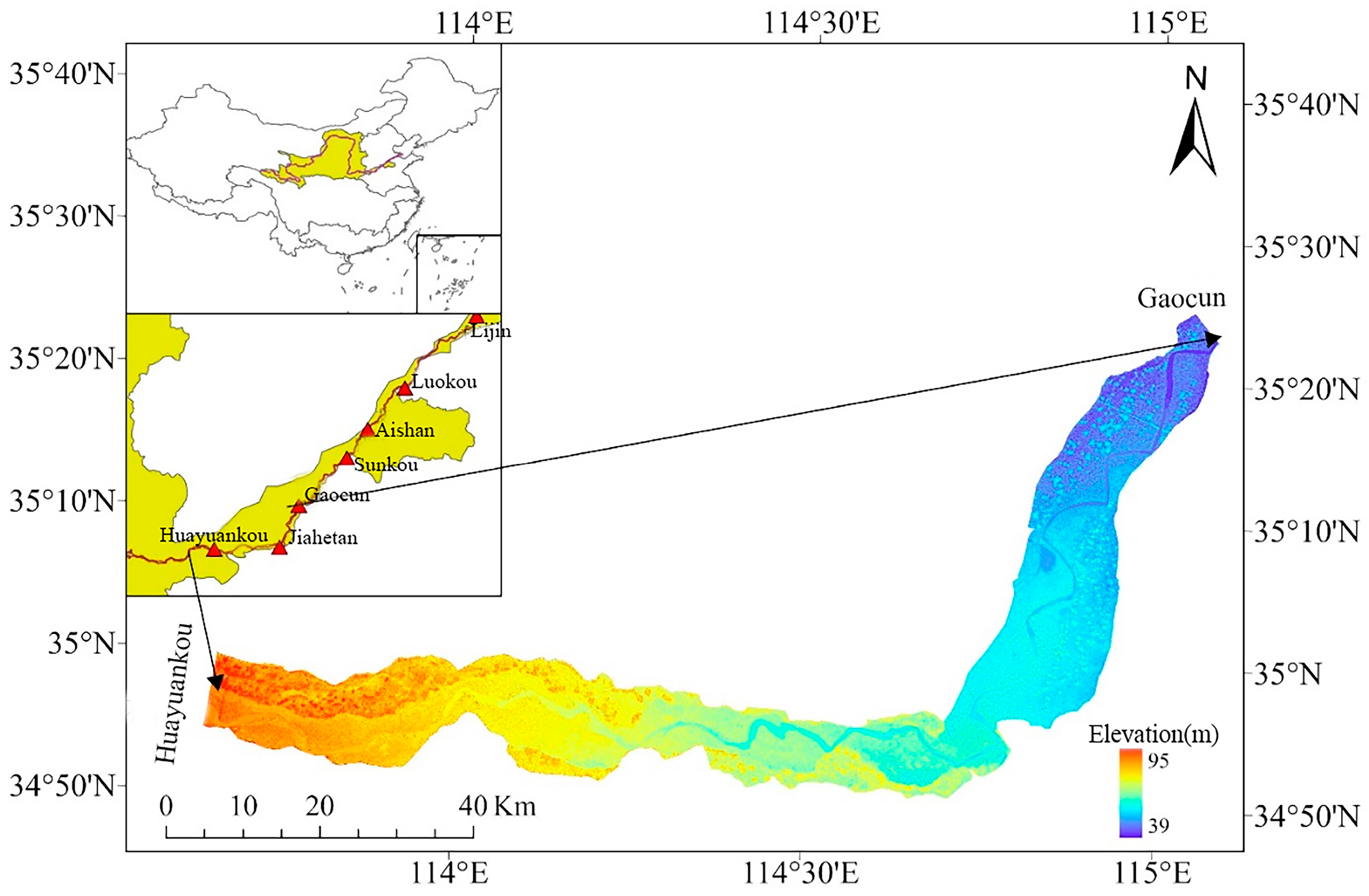
The study area is the reach of the lower Yellow River in China between Huayuankou and Gaocun, which represents a typical wandering river segment, as shown in Figure 1. This region lies within the North China Plain, covering an area of approximately 1695 km², with geographical coordinates ranging from 113°35′ E to 115°10′ E and 34°50′ N to 35°30′ N. The terrain exhibits a general trend of higher elevation in the west and lower elevation in the east. The climate is classified as a temperate monsoon type. The geomorphic types of the river channel are functionally classified into main river channels, floodplains, training and protection structures, productive embankments, roads, and farmland. The distance between the main embankments on both banks generally ranges from 5 km to 10 km, with the widest section reaching up to 24 km. The longitudinal slope of the river channel varies between approximately 2.65‱ and 1.72‱. The study area contains numerous floodplains, including fourteen floodplain zones such as Huayuankou, Changyuan, Yuanyang, and Dongming. Among these, the Yuanyang and Changyuan floodplains each cover an area exceeding 300 km², while the Fengqiu Backwater Area, WeiTan, and Dongming floodplain areas all have areas greater than 100 km².

2.2. Similarity Criterion of Experiment

Experiment focuses on the evolution of sediment-laden flow within the ecological protective forest area along the lower Yellow River embankment, including the hydrodynamic behavior of the flow and the mechanisms of sediment erosion and deposition. To accurately represent these processes, the experimental design must satisfy both hydrodynamic and sediment movement similarity criteria. Since the primary force governing flow movement is gravity, the Froude similarity criterion should be applied. Additionally, due to the presence of sediment, similarity in flow turbulence resistance must also be considered. Key similarity criteria for sediment transport include: bed load movement, suspended sediment transport, vertical distribution of sediment concentration, sediment-carrying capacity of the flow, and riverbed erosion and deposition patterns.

The following similarity criteria should be adhered to in the experimental design:

Similarity Criterion of Gravity:

$${\lambda }_V={\lambda }_H^{1/2}$$

(1)

Similarity Criterion of Flow Resistance:

$${\lambda }_n={\displaystyle \frac{1}{{\lambda }_V}}{\lambda }_H^{2/3}{\lambda }_J^{1/2}={\lambda }_H^{2/3}{\lambda }_L^{-1/2}$$

(2)

Similarity Criterion of Stream Sediment Transport:

$${\lambda }_s={\lambda }_{s^{*}}$$

(3)

Similarity Criteria of Sediment Suspension:

$${\lambda }_{\omega }={\lambda }_V{\left({\displaystyle \frac{{\lambda }_H}{{\lambda }_L}}\right)}^m$$

(4)

Similarity Criteria of Sediment Incipient Motion:

$${{\displaystyle \lambda }}_{Vc}={{\displaystyle \lambda }}_V$$

(5)

Time Similarity Criteria of Water Flow Movement:

$${{\displaystyle \lambda }}_{t1}={\displaystyle \frac{{{\displaystyle \lambda }}_L}{{{\displaystyle \lambda }}_V}}$$

(6)

Similarity Criteria of Riverbed Erosion and Deposition:

$${\lambda }_{t2}={\displaystyle \frac{{\lambda }_{\gamma 0}}{{\lambda }_s}}{\lambda }_{t1}$$

(7)

where λ_L is horizontal scale; λ_H is vertical scale; λ_V is average velocity scale of water flow; λ_n is roughness scale; λ_J is gradient scale; λ_s is sediment concentration scale of water flow; λ_s* is sediment-carrying capacity scale of water flow; λ_ω is sediment settling velocity scale; λ_Vc is sediment incipient velocity scale; λ_t1 is experimental water flow duration scale; λ_t2 is river bed deformation time scale; λ_γ0 is experimental dry bulk density scale of suspended sediment; and m is coefficient, commonly taken as 0.5 in Yellow River channel model experiments.

Based on field observations of the morphological characteristics of the ecological protective forests along the lower Yellow River, and in consideration of laboratory constraints and established scaling practices, the geometric scales for this generalized flume experiment were determined as λ_L = λ_H = 80. Other relevant scales were subsequently derived in accordance with the previously stated similarity criteria. The specific scaling ratios used in the experiment are provided in

Table 1. Similarity criterion summary.

Serial	Name	Sign	Value	Criterion
1	Horizontal scale	λL	80	Space limitation
2	Vertical scale	λH	80	Geometric characteristics of protective forest
3	Average velocity scale	λV	8.94	Gravity similarity criterion
4	Discharge scale ratio	λQ	57,243	Gravity similarity criterion
5	Roughness scale	λn	2	Similarity criterion of flow resistance
6	Water flow duration scale	λt1	8.94	Water flow movement time similarity criterion
7	Sediment concentration scale	λs	1	Sediment suspension similarity criterion
8	River bed deformation time scale	λt2	8.94	Similarity criterion of scouring and silting deformation of river bed

.

In addition to the similarity criteria outlined above, the experimental design should also adhere to the following constraints.

(1) Limitation of subcritical flow and supercritical flow

• subcritical flow:

  $$F_r={\displaystyle \frac{v}{gh}}<1$$

  (8)
• supercritical flow:

  $$F_r={\displaystyle \frac{v}{gh}}>1$$

  (9)

  where F_r is Froude number; v is cross-sectional mean velocity; g is gravity; and h is mean water depth.

(2) Laminar and turbulent flow restriction conditions

Natural flow exhibits two distinct regimes: laminar flow and turbulent flow, each with fundamentally different characteristics. Since the Reynolds number of natural flow typically exceeds the critical value, it is generally in a turbulent state. Therefore, the experimental flow should also be maintained in the turbulent regime, ensuring that the Reynolds number remains greater than the critical Reynolds number.

(3) Limitation of resistance square area

Natural water flow, particularly during flood seasons, typically falls within the resistance square area—a state of fully developed turbulence. Therefore, the experimental flow must also be in a fully turbulent regime, which requires the Reynolds number in the model to exceed the critical range of 1000 to 2000.

(4) Limitation of surface tension

Due to the cohesive forces between water molecules, surface tension develops at the interface with other media. To ensure that the experimental flow is not unduly influenced by surface tension effects, a minimum water depth of 1.5 cm must be maintained.

2.3. Experimental Arrangement

2.3.1. Experimental Flume

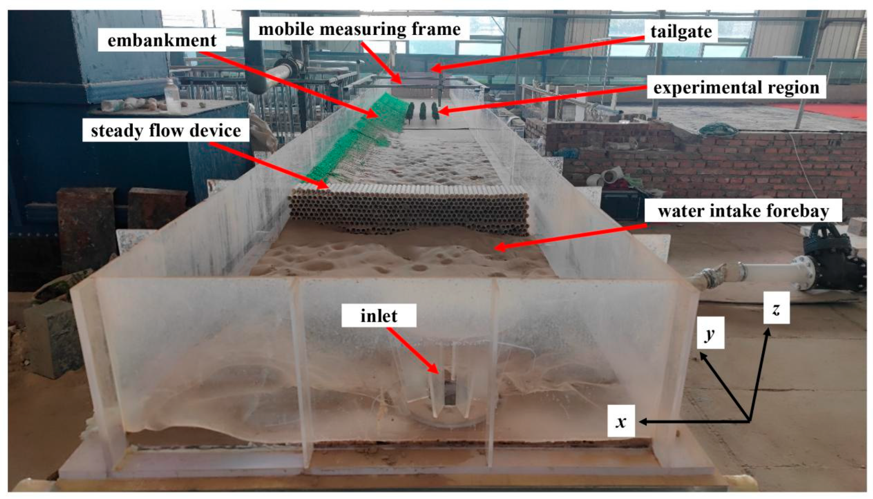
The experiment was conducted in the Hydraulics and River Regulation Laboratory at North China University of Water Resources and Electric Power. A scaled physical model of the flume was constructed according to the predetermined geometric scale, with the specific configuration adapted to the available site conditions, as illustrated in Figure 2.

The experimental system consists of three integrated components: a sediment–water mixing system, a water supply system, and a flume system. The main flume, constructed with smooth-surfaced plexiglass sidewalls and a high-density PVC rectangular base, measures 10 m in length, 1.0 m in width, and 0.35 m in height. Longitudinally, the flume was divided into five functional sections: the forebay, the front transition region, the experimental region, the rear transition region, and the withdrawal region. The forebay, situated between the inlet and the flow-stabilizing device, has dimensions of 1.0 m × 1.0 m × 0.2 m (L × W × H). Its primary function is to temporarily store and regulate the sediment-laden water delivered from the mixing tank via the supply system before it enters the experimental area.

A 20 cm long flow-stabilizing device was installed downstream of the forebay. This device was constructed from multiple PVC pipes, each with a diameter of 2 cm. During fabrication, the pipes were cut into 20 cm segments, arranged in tangential contact, and securely bonded using high-strength adhesive to form a compact honeycomb-structured bundle measuring 20 cm in both length and height. The primary function of this device is to dampen flow fluctuations and stabilize incoming currents. Water entering the forebay from the supply pipeline typically exhibits high turbulence intensity and complex flow behavior. The honeycomb configuration effectively dissipates these disturbances, promoting a more uniform flow profile essential for accurate hydraulic measurements in the experimental area. Inflow to the flume was regulated by an adjustable inlet valve, while a tailgate at the downstream end controlled the water level throughout the experiments.

2.3.2. Ecological Protective Forest Arrangement

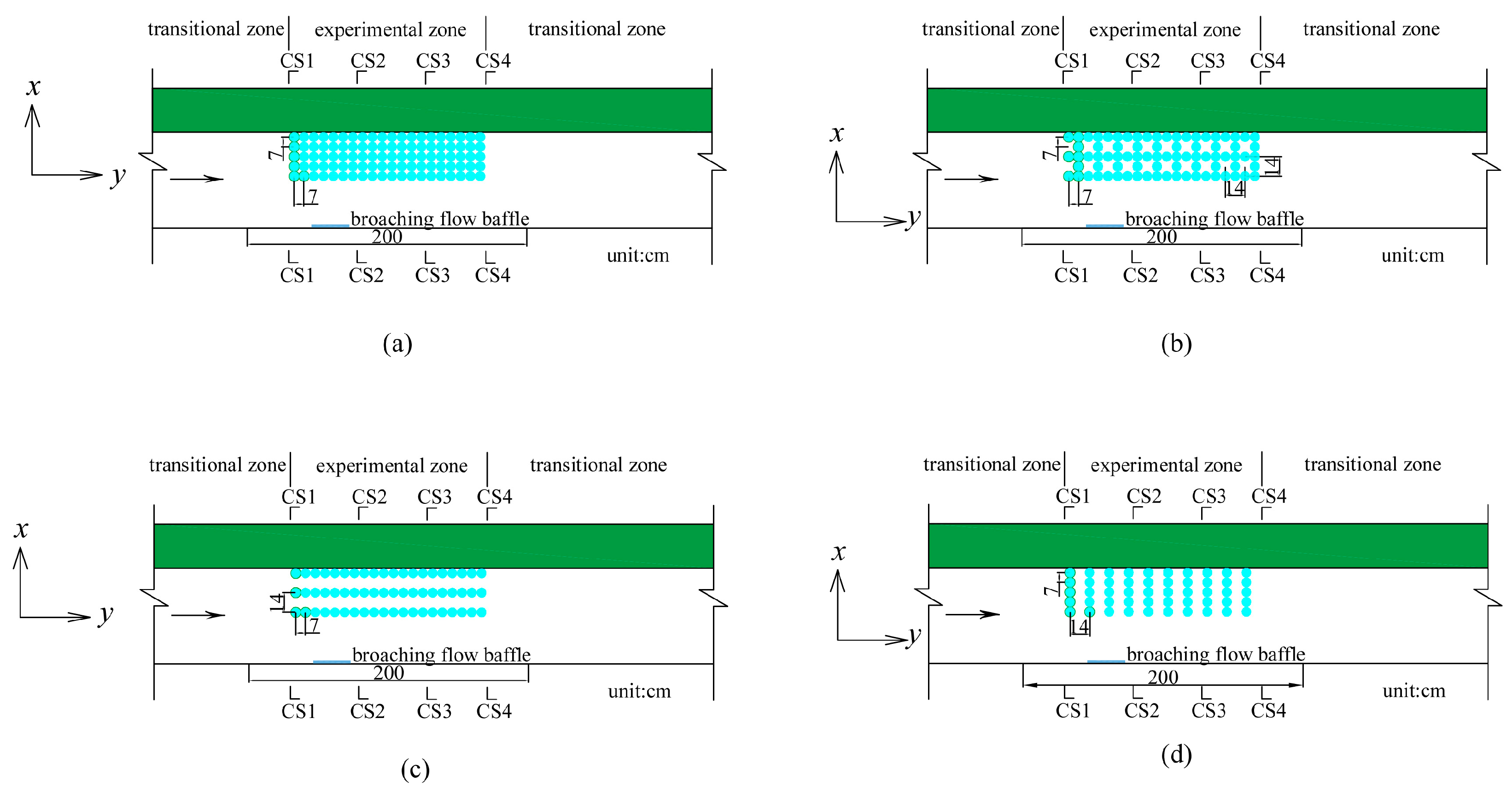
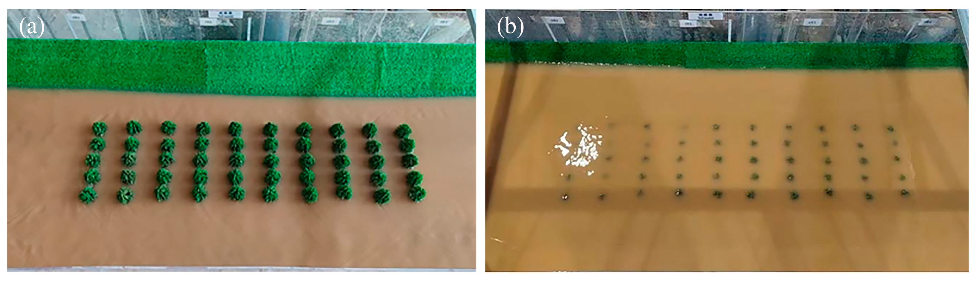
The ecological protective forest model was positioned 4.00–5.40 m downstream from the steady flow device, covering a length of 1.40 m and a width of 0.35 m. Depending on the spacing configuration, the model consisted of 10 rows in the transverse (x) direction and 20 rows along the streamwise (y) direction. Four distinct arrangement patterns were implemented, as illustrated in Figure 3:

Arrangement A1: The ecological protective forest models are arranged in 5 transverse rows, with uniform center-to-center spacing of 7 cm in both transverse and longitudinal directions.

Arrangement A2: Derived from A1 by removing all even-numbered rows along the longitudinal direction. This results in alternating transverse center spacings of 7 cm and 14 cm, and longitudinal spacings of 7 cm and 14 cm.

Arrangement A3: Derived from A1 by removing even-numbered rows in the transverse direction, yielding a transverse center spacing of 14 cm and a longitudinal spacing of 7 cm.

Arrangement A4: Derived from A1 by removing even-numbered rows along the longitudinal direction, resulting in a transverse center spacing of 7 cm and a longitudinal spacing of 14 cm.

The layout of measurement sections for flow velocity and sediment concentration is illustrated in Figure 3. Four cross-sections (CS1–CS4) were established along the streamwise direction (y-axis) within the protective forest area. CS1 is situated upstream of the leading edge of the forest; CS2 and CS3 are located inside the forest, with CS2 at one-third and CS3 at two-thirds of the total forest length; CS4 is positioned downstream of the trailing edge.

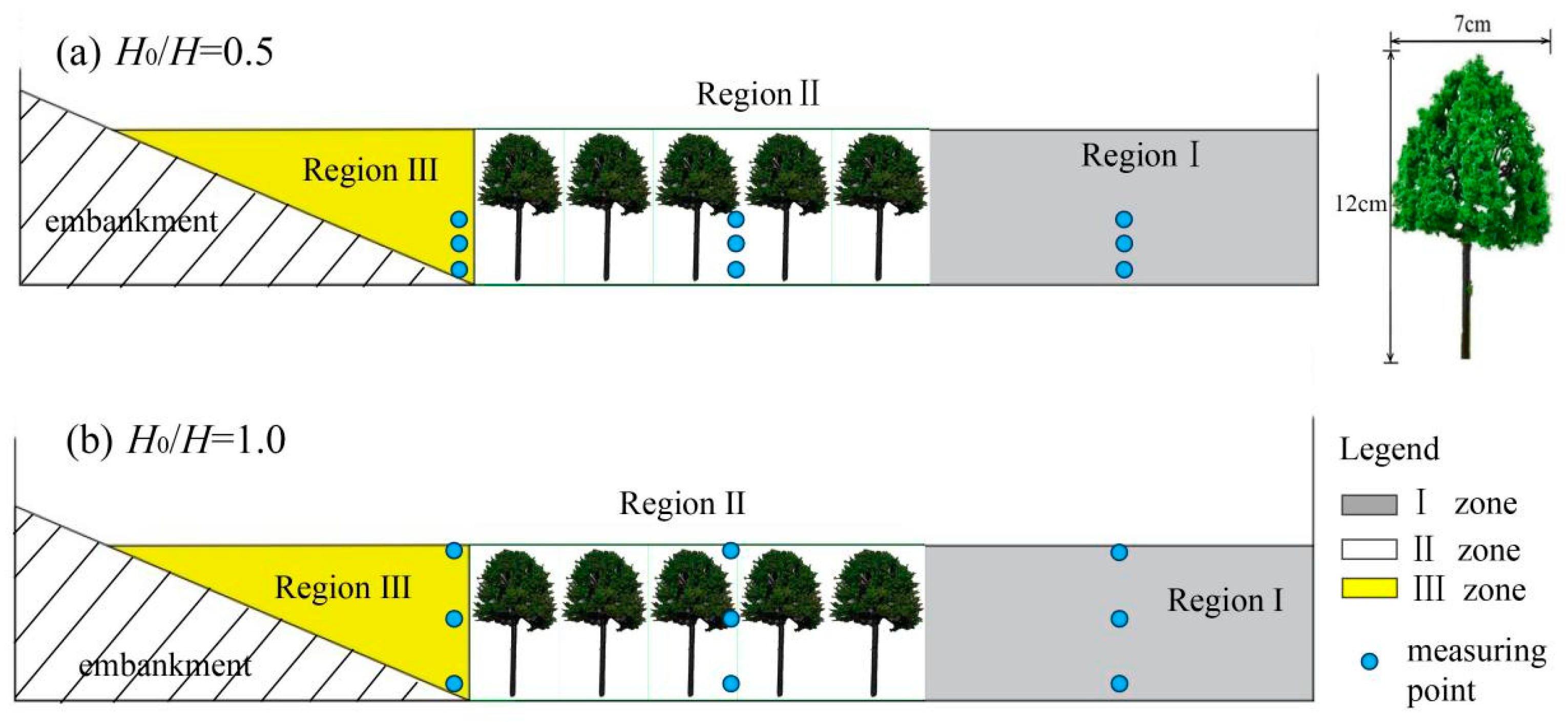
The ecological protective forest model was generalized based on typical tree species identified in the Dongming Beach area. Field investigations at Dongming Beach indicate that the dominant species used in these ecological protective forests are Fraxinus chinensis and Sophora japonica. Accordingly, the model trees were designed at experimental scale using morphological parameters representative of these species, which is shown in Figure 4, with a vertical height of 12 cm, a maximum crown width of 7 cm horizontally, and a trunk diameter of approximately 4 mm. It is necessary to clarify that real tree species are simplified into rigid geometric models. To some extent, the omission of flexibility, porosity variation, branch motion, and seasonal foliage strongly limits ecological realism. This simplification requires further quantitative framing. Specifically, willow which was identified as the most effective species in Zhang et al. [7] is highly flexible. Under high-flow conditions, flexible vegetation reconfigure such as bend and streamline in response to flow drag, which reduces their frontal area and drag coefficient relative to rigid vegetation of the same size [35,36,37]. Luhar and Nepf [37,38] proposed the concept of “effective length” (l_e) to quantify this drag reduction, showing that flexible blades generate substantially lower drag than rigid blades at high Cauchy numbers (Ca ≫ 1). Chapman et al. [39] experimentally compared rigid and flexible cylindrical obstructions of identical size and found that flexibility significantly reduces measured drag forces. In the context of the present study, this implies that our rigid model trees likely overestimate flow resistance and, consequently, the sediment deposition promotion effect under submerged or high-velocity conditions. Lower velocities and partially submerged conditions may reduce this bias, but the direction of error is consistently towards overestimation of deposition enhancement.

Figure 4 illustrates the experimental zone configuration and measurement point locations under varying submergence conditions. The flume was divided into three regions: Region I extends from the right edge of the forest to the right flume wall; Region II corresponds to the forested area; and Region III spans from the left forest edge to the left embankment, featuring a triangular cross-section. In each measurement section, three points were arranged along the transverse direction (x-axis) at normalized positions of b/B = 0.15, 0.37, and 0.65, where b denotes the distance from the point to the right flume wall and B represents the bottom width of the flume. Define submergence degree as the ratio of water depth (H₀) to the height of the protective forest model (H). Two submergence degrees were set as 0.5 and 1.0. Along the vertical direction (z-axis), three measurement points were set at each transverse location. For a submergence degree of 0.5, the vertical locations of measurement points were Z/H₀ = 0.167, 0.5, and 0.833; for a submergence degree of 1.0, the locations of measurement points were Z/H₀ = 0.083, 0.5, and 0.917, where Z is the height above the flume bed and H₀ is the water depth.

2.3.3. Selection of Sediment

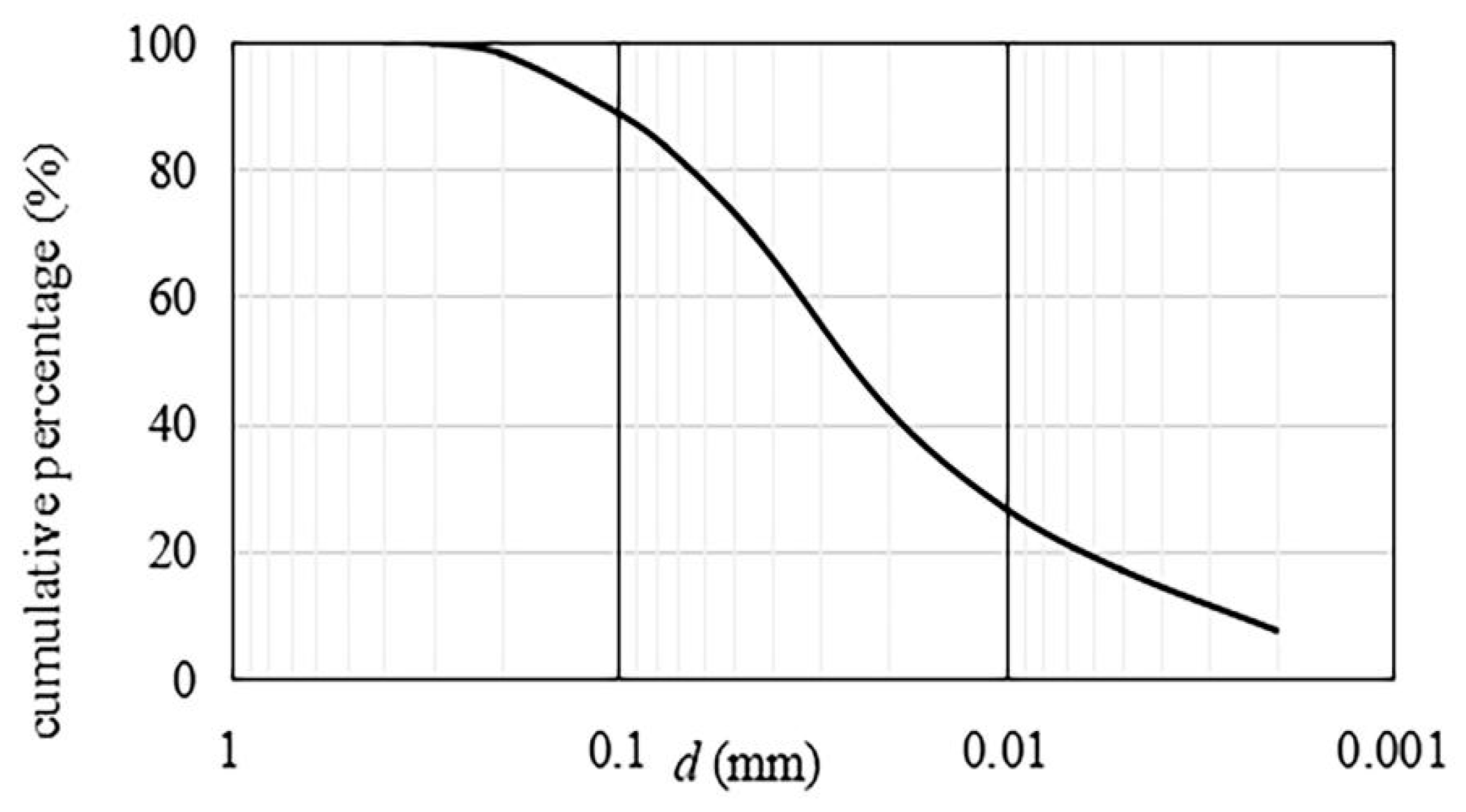
The sediment in the lower Yellow River consists predominantly of fine suspended particles, making it difficult to source suitable experimental sediment that strictly conforms to the scaled size requirements. In line with previous research and in consideration of the experimental objectives, natural sediment collected from the lower Yellow River was used in this study. The particle size distribution of the natural sediment was determined using a BT-9300ST laser particle size analyzer (Bettersize Instruments Ltd., Dandong, China). The gradation curve is presented in Figure 5, and the median particle size (d₅₀) was measured as 0.0255 mm. It should be noted that natural sediment was used because ideal scaled sediment was unavailable. While understandable, this creates scaling inconsistency.

2.4. Experimental Scenario

Considering the combination of water and sediment in natural rivers, three characteristic water–sediment combinations were adopted: low flow with low sediment (Q = 5 L/s, S = 5 kg/m³), high flow with low sediment (Q = 10 L/s, S = 5 kg/m³), and high flow with high sediment (Q = 10 L/s, S = 10 kg/m³). Under varying inflow and sediment conditions, a total of 24 experimental scenarios were conducted, as summarized in

Table 2. Basic hydraulic parameters.

RUN	Vegetation Height (cm)	Arrangement	Submergence Degree	Mean Water Depth (cm)	Discharge (L/s)	Sediment Concentration (kg/m3)	ρv (%)	ρL (%)
1	12	A1	0.5	6	5	5	2.78	0.26
2					10	5
3					10	10
4			1	12	5	5	12.34	78.5
5					10	5
6					10	10
7	12	A2	0.5	6	5	5	2.78	0.21
8					10	5
9					10	10
10			1	12	5	5	12.34	62.8
11					10	5
12					10	10
13	12	A3	0.5	6	5	5	1.67	0.15
14					10	5
15					10	10
16			1	12	5	5	7.41	47.1
17					10	5
18					10	10
19	12	A4	0.5	6	5	5	2.78	0.15
20					10	5
21					10	10
22			1	12	5	5	12.34	47.1
23					10	5
24					10	10

. Table 2 lists the key physical parameters for each experiment, including vegetation arrangement, water depth, submergence degree, discharge, sediment concentration, vertical vegetation density, and horizontal vegetation density. In all scenarios, the water depth is greater than 1.5 cm, satisfying the surface tension requirement.

The vertical vegetation density, ρ_v, is defined as the ratio of the total longitudinal projected area, A_h, of all vegetation elements on the flume cross-section to the cross-sectional flow area, A₁, measured at the center of the vegetation region. That is:

$${\rho }_v={\displaystyle \frac{A_h}{A_1}}$$

(10)

The horizontal vegetation density, ρ_L, is defined as the ratio of the total projected area A_L of all vegetation elements on the riverbed to the total bed area A₂ within the protective forest region, expressed as:

$${\rho }_L={\displaystyle \frac{A_L}{A_2}}$$

(11)

Based on the experimental design and layout described previously, preliminary pretests were first carried out in order to detect any possible problems such as water leakage. Refinements were made to address issues observed during the pretests before formal experiments were conducted. The experimental procedure consisted of two main phases: pre-experimental preparation and experimental execution. The specific operational steps for each scenario were as follows:

(1) Preparation of Sediment-Laden Flow in the Mixing Tank

According to the target sediment concentration specified in the experimental design, a predetermined volume of clear water was added to the mixing tank, followed by a measured quantity of sediment. The mixing system was then activated and run for a sufficient period to achieve a homogeneous sediment–water mixture. Sediment concentration was verified using a pycnometer and an electronic balance. If the measured concentration was lower than the design value, additional sediment was added and mixed thoroughly before re-measurement. Conversely, if the concentration exceeded the target, clear water was added incrementally until the desired concentration was attained.

(2) Arrangement of the Ecological Protective Forest

To secure the model trees, a PVC board pre-drilled with holes was fixed to the flume bed. Following the experimental layout plan, tree models were inserted into the holes and firmly fastened to prevent displacement under flow conditions.

(3) Flume filling and Flow conditioning

The sediment–water mixing system was restarted and operated until homogeneity was re-achieved. Sediment concentration was checked again to confirm it met the experimental requirements. The water supply pump was then started to fill the flume gradually. Discharge was regulated via a control valve until the target flow rate was reached. The tailgate at the downstream end was adjusted to maintain a constant water depth along the flume.

(4) Experimental observation and Data Collection

Once steady flow conditions were established, velocity was measured using an electromagnetic current meter (Nanjing Huanyang Automation Co., Ltd., Nanjing, China), and sediment concentration samples were collected with a pycnometer. A camera was used to document flow patterns and related phenomena. After one hour of test duration, sediment deposition thickness within the experimental reach was measured with a calibrated scale.

(5) Post-Experiment Cleanup

After completing the measurements, accumulated sediment was thoroughly flushed from the flume using clean water. Measuring instruments were re-positioned and re-calibrated as necessary before starting the next experimental run.

2.5. Experimental Measuring Instrument

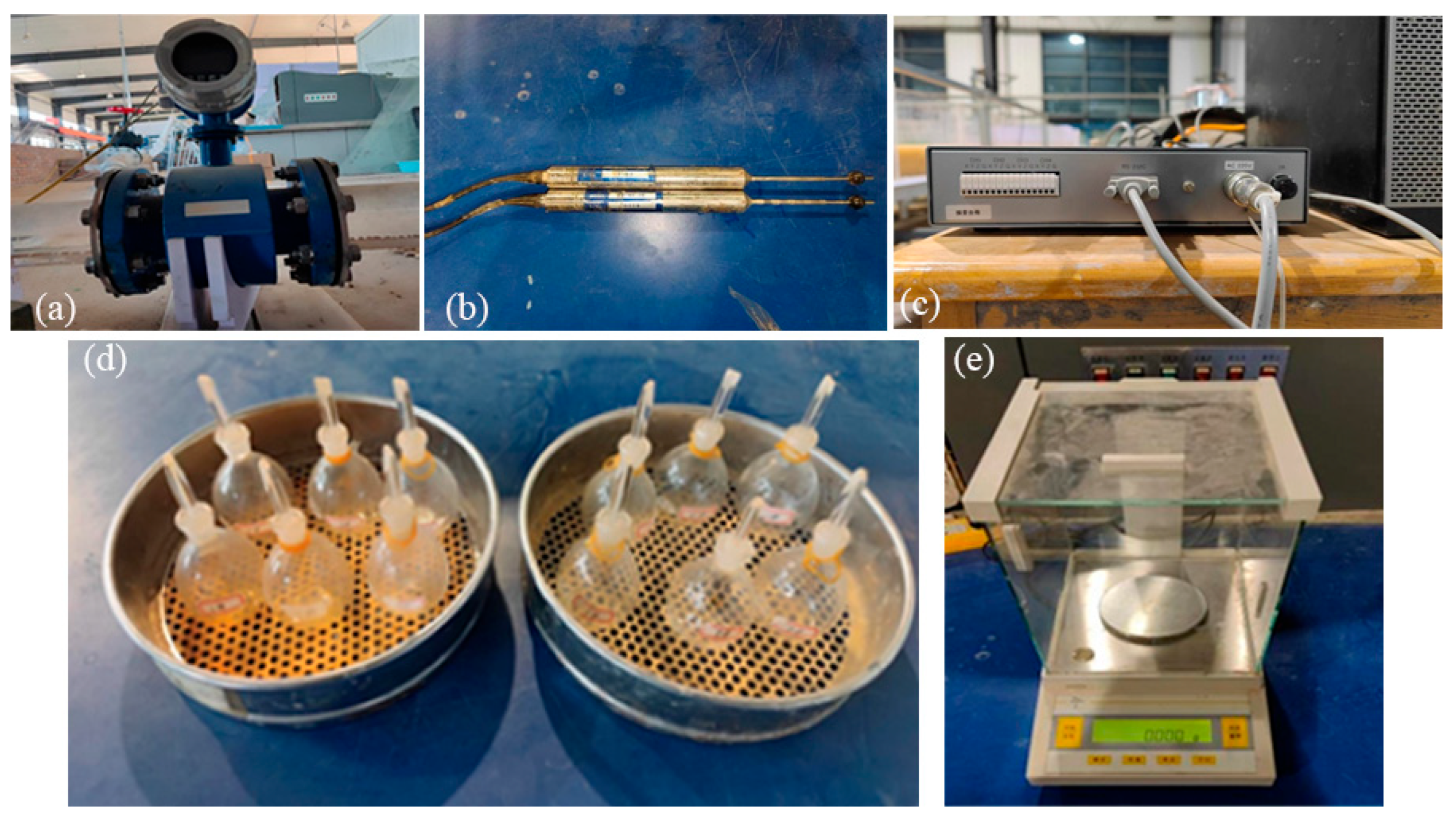
Discharge, flow velocity, water level, and sediment concentration were measured using an electromagnetic flowmeter (Nanjing Huanyang Automation Co., Ltd., Nanjing, China), an electromagnetic current meter, a ruler, a pycnometer, and an electronic balance, respectively, with a water pump serving as the water supply equipment. The inflow to the flume was measured using an integrated digital electromagnetic flowmeter (Model HY-LDG, Nanjing Huanyang Automation Co., Ltd. (Nanjing, China); see Figure 6a). Flow velocity in the experimental area was measured using a laboratory electromagnetic current meter (Model LS-606, Nanjing Huanyang Automation Co., Ltd., Nanjing, China; see Figure 6b,c). The water supply system employed a single-phase submersible electric pump (Model: QDX55-2-2.2, Changzhou Wanhe Electromechanical Co., Ltd., Changzhou, China). Key specifications include a power rating of 2.2 kW, supply voltage of 220 V, operating frequency of 50 Hz, pump head of 5 m, rotational speed of 2860 r/min, rated discharge capacity of 55 m³/h, and outlet diameter of 100 mm.

A ruler with an accuracy of 1 mm was used for length measurements. The ruler was affixed to both the three-dimensional measuring frame and the side of the glass flume using double-sided adhesive tape to control the displacement of measuring instruments and monitor water depth. Sediment concentration was determined using twelve 50 mL pycnometers, numbered #1 to #12, as shown in Figure 6d. Prior to measurement, each pycnometer was calibrated by filling it with clear water and repeatedly weighing it on an electronic balance; the average value from multiple calibrations was taken as the calibration constant. During sediment concentration measurement, each pycnometer was filled with sediment-laden water and weighed. The net mass of suspended sediment was obtained by subtracting the calibration constant from the total weight. Sediment concentration was then calculated by dividing this net mass by the volume of the pycnometer. An electronic balance (Model JA2003, Shanghai Sunny Hengping Scientific Instrument Co., Ltd. (Shanghai, China); maximum capacity 200 g, measurement accuracy ±0.001 g) was used for all mass measurements, as illustrated in Figure 6e.

3. Results and Analysis

3.1. Submergence Process of Ecological Protective Forest

The submergence process of ecological protective forests unfolds as follows: when sediment-laden flow enters the forested area, it is initially influenced by the trunks, generating a flow pattern analogous to pier scour in hydraulic engineering. As water depth increases, the canopy becomes progressively submerged, leading to more complex flow–vegetation interactions. The process continues until the entire protective forest model is fully submerged and can be divided into three distinct stages:

(1) Trunk Submergence Stage

After passing through the flow stabilization device, the water enters a transition section where partial sediment deposition occurs. Upon reaching the ecological protective forest area, flow first submerges the lower trunk region and gradually covers the entire trunk. Under partial submergence conditions, once the trunk is fully submerged, the water depth remains constant throughout the remainder of the experiment. During this stage, trunk obstacles redirect the flow. Based on classical bluff-body flow theory [23], this may create accelerated velocities and reduced pressure regions around the cylinders, potentially leading to vortex formation on both sides of trunks, with faster circum-trunk flow and lower local pressure. However, no direct turbulence measurements (Reynolds stresses or turbulent kinetic energy) were made in this study; these inferred flow features are drawn from the literature rather than from our experimental data.

(2) Canopy Submergence Stage

With further increase in water depth, the canopy becomes progressively inundated. Branches and leaves within the canopy region obstruct forward flow, generating localized eddies and circumfluent patterns. The complex architecture of the canopy significantly modifies flow pathways and velocity distributions, creating heterogeneous flow conditions through the vegetation layer.

(3) Post-Submergence Stable Stage

Once the canopy is fully submerged and water depth stabilizes, constant flow conditions are established for experimental measurements. During this stage, flow velocities become more uniform and stable, with minimal kinetic energy loss and well-developed flow patterns. Sediment deposition processes attenuate, with suspended sediments gradually settling both within the forested area and in upstream regions. Figure 7 illustrates the protective forest under semi-submerged and fully submerged conditions.

This study specifically examines the third stage described above namely the Post-Submergence Stable Stage. Flow velocity, sediment concentration, and sediment deposition within the protective forest area were measured after a 1 h period. Based on these measurements, the hydraulic characteristics and sediment deposition patterns across different cross-sections were systematically analyzed.

3.2. Influence of Arrangement Patterns on Sediment Deposition Effect

Identifying which ecological protective forest arrangement yields superior sediment deposition effects represents a key research focus. A single-factor analysis was adopted, maintaining constant water–sediment conditions (discharge Q = 10 L/s, sediment concentration S = 5 kg/m³). This configuration was selected based on hydrological considerations: although extreme floods remain possible in the lower Yellow River, the probability of high-sediment overbank floods has significantly decreased due to water conservancy projects and soil conservation measures [7]. Furthermore, during floodplain inundation, whether the flow evolves into oblique or transverse river patterns, it ultimately stabilizes into a prolonged embankment-parallel flow condition, making the selected scenario hydrologically representative.

Figure 8 presents the deposition thickness of the four arrangements at semi-submerged state. Different arrangements exhibited distinct deposition patterns. Arrangement A1, with the highest vegetation density, showed that in semi-submerged conditions—where only trunks interact with flow—the interference with sediment-laden flow remained limited. Deposition primarily occurred upstream of the forest due to backwater formation and associated flow deceleration, reducing sediment transport capacity. Comparative analysis revealed that greater vegetation density generally promoted increased sediment deposition. Under embankment-parallel flow conditions, when longitudinal spacing (l_y) exceeded transverse spacing (l_x), deposition concentrated upstream; conversely, when l_y < l_x, sediment transport extended further downstream with more uniform thickness distribution.

Figure 9 illustrates the deposition thickness for the four arrangements at full submerged state. All configurations enhanced sediment deposition compared to non-vegetated areas, though their effectiveness varied significantly. In fully submerged conditions, both trunks and canopy interact with the sediment-laden flow, with the canopy exhibiting a more pronounced flow-blocking effect. This results in a more evident backwater phenomenon upstream, a greater reduction in flow–sediment transport capacity, and consequently intensified deposition with increased thickness. The deposition patterns of the four arrangements showed minimal variation under full submergence, with upstream deposition consistently exceeding downstream levels. Overall, arrangement A1 yielded the maximum deposition thickness, followed by A2 and A4, while A3 produced the least. Deposition thickness generally increased with protective forest density. Furthermore, under embankment-parallel flow conditions, configurations with transverse spacing (l_x) smaller than longitudinal spacing (l_y) proved more effective in promoting sediment deposition.

The amount of sediment deposition upstream is greater than that downstream. This may be due to the fact that after upstream flow carries sediment into the experimental area, the flow velocity drops rapidly due to obstruction by the vegetation structure (e.g., dense plant stems), causing coarse sediment to deposit preferentially at the entrance. As the flow gradually recovers its energy along the path, the sediment transport capacity downstream becomes relatively stronger, resulting in a decreasing pattern of sedimentation. As the flow’s ability to transport sediment decreases, partial deposition occurs on the riverbed—a phenomenon consistent with existing research findings [16,17,29].

The deposition effects of different arrangements at semi-submerged state (H₀/H = 0.5) and full submerged state (H₀/H = 1.0) are shown in

Table 3. Summary of deposition effects for the four arrangement patterns.

Submergence Degree	Cross-Section	Arrangement A1		Arrangement A2		Arrangement A3		Arrangement A4
		Deposition Thickness (mm)	Deposition Rate (%)	Deposition Thickness (mm)	Deposition Rate (%)	Deposition Thickness (mm)	Deposition Rate (%)	Deposition Thickness (mm)	Deposition Rate (%)
H0/H = 0.5	CS1-Region I	2.3	9.13	2.2	5.91	2.07	3.86	2.12	6.13
	CS1-Region II	2.51		2.33		2.15		2.25
	CS2-Region I	2.06	8.25	2.25	4.89	2.05	4.39	2.11	5.21
	CS2-Region II	2.23		2.36		2.14		2.22
	CS3-Region I	2	7	2.15	6.05	2.03	4.93	2.08	5.29
	CS3-Region II	2.14		2.28		2.13		2.19
	CS4-Region I	1.78	6.18	2.1	4.76	2.01	5.47	2.05	4.88
	CS4-Region II	1.89		2.2		2.12		2.15
H0/H = 1.0	CS1-Region I	3.77	12.47	3.6	11.94	3.49	8.88	3.52	11.36
	CS1-Region II	4.24		4.03		3.8		3.92
	CS2-Region I	3.74	12.57	3.57	11.76	3.43	9.04	3.5	10.86
	CS2-Region II	4.21		3.99		3.74		3.88
	CS3-Region I	3.62	11.33	3.51	10.83	3.41	8.5	3.46	10.4
	CS3-Region II	4.03		3.89		3.7		3.82
	CS4-Region I	3.5	9.14	3.49	8.88	3.39	7.96	3.43	8.75
	CS4-Region II	3.82		3.8		3.66		3.73

. Here, define the deposition rate as the ratio of the difference in average deposition thickness between Region II (forested) and Region I (non-forested) to the average deposition thickness in Region I (the same applies hereafter). Overall, deposition patterns vary across the four measurement sections for each arrangement. However, within the same section, arrangement A1 consistently exhibits a higher deposition rate than the other three arrangements, indicating its superior effectiveness in promoting sediment deposition. This suggests that higher density of ecological protective forest increases the flow-blocking area, thereby enhancing sediment retention. At full submerged state, both the trunk and canopy contribute to flow resistance, with the canopy playing a more significant role in flow blocking. Consequently, deposition thickness values under full submergence exceed those observed under partial submergence.

3.3. Sediment Deposition Promotion Effect of Ecological Protective Forests

When over-bank floods reach ecological protective forests along embankments, significant alterations occur in flow velocity and sediment concentration—key parameters governing riverbed evolution in these areas. To isolate the individual effects of hydrological variables, arrangement A1 was selected ensuring single-factor analysis by eliminating confounding variables. Embankment erosion is closely associated with near-bank flow velocity, which plays a determining role in bank toe scouring. To quantify this effect, we define reduction rate of flow velocity as the ratio of velocity reduction at a given measuring point to the reference velocity at the corresponding point in non-vegetated areas. Since cross-sections CS2 and CS3 exhibit similar flow characteristics within the forested region, CS2 was selected as representative for analyzing near-bank velocity distribution.

3.3.1. Flow Velocity Characteristics

Velocity distribution at cross-section CS2 at semi-submerged state for low flow with low sediment (Q = 5 L/s, S = 5 kg/m³) is shown in Figure 10a–c. Here, b denotes the transverse distance from the measurement point to the right flume wall, B represents the bottom width of the flume, while x (transverse), y (streamwise), and z (vertical) define the coordinate directions. The time-averaged velocity components are denoted as v_x, v_y, and v_z, respectively. Significant differences in velocity magnitude were observed among directions, with stream-wise velocity (v_y) substantially exceeding transverse (v_x) and vertical (v_z) components across all regions: non-forested Region I, forested Region II, and embankment Region III. This attenuation occurs because partial submergence limits flow–vegetation interaction primarily to trunk-induced drag, analogous to flow around cylindrical structures. The presence of both positive and negative values in v_x and v_z reflects the complex flow patterns induced by trunk-scale turbulence and secondary circulation. Consistent with previous studies [15,25], such patterns are often attributed to trunk-scale turbulence and secondary circulation in vegetated flows. However, because we did not measure fluctuating velocity components, these interpretations remain inferences from the literature rather than direct evidence from our data.

For high flow with low-sediment conditions (Q = 10 L/s, S = 5 kg/m³, Figure 10d–f), a similar velocity structure was observed. The stream-wise velocity component remained dominant in Regions I, II, and III, respectively. The velocity in Region II was 24.1% and 18.8% lower than in Regions I and III, highlighting the forest’s flow-retarding effect. Although the vertical distribution of v_x was consistent in Regions I and II, it differed in Region III, though all remained positive. Vertical velocity (v_z) showed similar distribution trends across regions but varied in magnitude and direction.

For high flow with high-sediment conditions (Q = 10 L/s, S = 10 kg/m³, Figure 10g–i), the velocity distribution again exhibited the same directional pattern. Stream-wise velocities with Region II show a 25.9% and 17.1% reduction compared to Regions I and III. Although the overall distribution patterns showed minimal variation across regions, the stream-wise velocity v_y in the forested Region II was consistently lower. Differences in v_x distributions reflect the distinct boundary conditions of each region, whereas v_z distributions remained broadly similar.

Velocity distribution at cross-section CS2 at full submerged state for low flow with sediment conditions (Q = 5 L/s, S = 5 kg/m³) is shown in Figure 11a–c, with symbols and variable definitions consistent with previous figures. On a given measurement line, the stream-wise velocity (v_y) again differed substantially from the transverse (v_x) and vertical (v_z) components. The vertical distribution of v_y in Region II (forested) diverged notably from that in Regions I (non-forested) and III (embankment). While velocities in Regions I and III generally followed a logarithmic profile, Region II exhibited a distinct velocity minimum within the canopy layer. Specifically, the minimum v_y value occurred at Z/H₀ = 0.5 in Region II, representing reductions of 77.1% and 73.1% compared to the same relative height in Regions I and III, respectively. At this position, v_y was comparable in magnitude to v_x and v_z, indicating a loss of stream-wise dominance. This pattern reflects the pronounced flow-blocking effect of the canopy under full submergence. The conical geometry of the model canopy, with its largest cross-sectional area at the base, explains the velocity minimum observed at mid-depth. This is consistent with the characteristic velocity profile commonly reported in vegetated flows found by Wang et al. [25]. Overall, velocities v_x and v_y values throughout the experimental area are generally lower than those observed at semi-submerged state.

Under high flow with low-sediment conditions (Q = 10 L/s, S = 5 kg/m³, Figure 11d–f), the velocity distribution followed a similar pattern. Regions I and III again exhibited comparable distributions, with v_y generally adhering to a J-shaped (logarithmic) profile. In contrast, Region II showed a distinct v_y minimum at Z/H₀ = 0.5, corresponding to reductions of 74.1% and 68.3% relative to Regions I and III, respectively. At this depth, v_y was again similar in magnitude to the transverse and vertical components. Region II consistently exhibited the lowest velocities, with the canopy reducing the depth-averaged v_y by an average of 48.7%. The maximum flow resistance occurred at the base of the conical canopy, leading to the velocity minimum at Z/H₀ = 0.5.

Under high-flow and sediment conditions (Q = 10 L/s, S = 10 kg/m³, Figure 11g–i), the velocity distribution remained consistent with the previous scenarios. Regions I and III maintained logarithmic-type velocity distributions, while Region II displayed a distinct velocity minimum within the canopy and an S-shaped vertical profile. The minimum v_y value occurred at Z/H₀ = 0.5, representing decreases of 69.8% and 64.3% compared to the same position in Regions I and III. At this point, v_y was again comparable to v_x and v_z. No clear patterns were observed in the distributions of v_x and v_z, though v_x remained positive throughout, while v_z exhibited both positive and negative values, indicating complex secondary motions.

3.3.2. Sediment Concentration Distribution

Figure 12a,b present sediment concentration distribution within the protective forest area under different submergence degrees under low flow and sediment conditions (Q = 5 L/s, S = 5 kg/m³). At both submerged states, the vertical distribution exhibited a consistent pattern, with lower concentrations near the surface and maximum values at the bottom layer. At a submergence degree of H₀/H = 0.5, the depth-averaged sediment concentrations along cross-sections CS1 to CS4 were 4.36 kg/m³, 4.21 kg/m³, 4.01 kg/m³, and 3.79 kg/m³, respectively. This indicates a progressive downstream decrease in sediment concentration as the sediment-laden flow traveled through the protective forest area. Similarly, under full submergence (H₀/H = 1.0), the depth-averaged concentrations at CS1 to CS4 measured 4.29 kg/m³, 4.16 kg/m³, 4.11 kg/m³, and 4.00 kg/m³, respectively, confirming the same longitudinal decreased pattern during flood passage through the forested region.

Figure 12c,d illustrate the sediment concentration distribution in the protective forest area under high-flow, low-sediment conditions (Q = 10 L/s, S = 5 kg/m³) for different submergence degrees. At both submerged states, the vertical distribution pattern remains consistent with previous observations, characterized by lower concentrations near the surface and maximum values near the bed. A clear longitudinal decay in sediment concentration is observed through the protective forest reach. At semi-submerged state of H₀/H = 0.5, the depth-averaged sediment concentrations along cross-sections CS1 to CS4 were 4.00 kg/m³, 3.73 kg/m³, 3.63 kg/m³, and 3.53 kg/m³, respectively. At full submerged state (H₀/H = 1.0), the corresponding depth-averaged values measured 3.99 kg/m³, 3.89 kg/m³, 3.74 kg/m³, and 3.64 kg/m³.

Figure 12e,f present the sediment concentration distribution within the protective forest area under high-flow, high-sediment conditions (Q = 10 L/s, S = 10 kg/m³). Consistent with previous scenarios, the vertical distribution under both submergence states shows lower concentrations near the surface and higher concentrations near the bed. A progressive longitudinal decay in sediment concentration is also observed along the protective forest reach. At semi-submerged state of H₀/H = 0.5, the depth-averaged sediment concentrations at cross-sections CS1 through CS4 were 5.17 kg/m³, 4.97 kg/m³, 4.96 kg/m³, and 4.91 kg/m³, respectively. At full submerged state (H₀/H = 1.0), the corresponding values measured 5.34 kg/m³, 5.23 kg/m³, 5.11 kg/m³, and 4.68 kg/m³.

3.3.3. Effects on Sediment Deposition Promotion

Deposition thickness serves as a key indicator for evaluating the sediment retention effectiveness of ecological protective forests along embankments. For low flow with sediment conditions (Q = 5 L/s, S = 5 kg/m³), the deposition thickness contours derived from post-experiment riverbed topography were shown in Figure 13, with (a) and (b) showing semi-submerged and full submerged states, respectively. Both submergence degrees resulted in net deposition throughout the experimental area, with Region II (forested) exhibiting greater deposition thickness than Region I (non-forested). Spatially, upstream deposition consistently exceeded downstream levels. At semi-submerged state, the average deposition thickness reached 4.35 mm in Region II compared to 3.93 mm in Region I, representing a 10.7% enhancement due to the protective forest. Full submergence yielded greater absolute thicknesses (6.13 mm in Region II vs. 5.30 mm in Region I) and a higher promotion effect of 15.6%. This difference arises because semi-submerged state limits flow–vegetation interaction primarily to trunk-induced resistance, which is relatively minimal given the small trunk diameters. In contrast, full submergence engages the dense canopy, creating substantially greater flow resistance and velocity reduction. The consequent decrease in sediment transport capacity promotes more pronounced deposition in the forested region.

For high-flow with low-sediment conditions (Q = 10 L/s, S = 5 kg/m³, Figure 13c,d), net deposition persisted under both submergence states, with Region II again showing greater thickness than Region I. At semi-submerged state, average thicknesses measured 2.22 mm (Region II) and 1.84 mm (Region I), corresponding to a 20.6% enhancement. Full submergence yielded 4.08 mm and 3.55 mm, respectively, with a 14.9% promotion effect. Compared to semi-submergence, full submergence shifted the deposition pattern downstream in the y-direction while reducing its transverse extent. These mechanisms align with those observed under low-flow conditions. The greater discharge in this scenario enhanced sediment transport capacity, resulting in overall thinner deposits despite maintained deposition promotion of approximately 15%.

For high-flow and sediment conditions (Q = 10 L/s, S = 10 kg/m³, Figure 13e,f), the deposition pattern remained consistent with previous scenarios in terms of zonal and spatial distribution. Semi-submergence produced average thicknesses of 7.34 mm (Region II) and 6.60 mm (Region I), an 11.2% enhancement. Full submergence resulted in 10.81 mm and 10.12 mm, respectively, with a 6.8% promotion effect. Unlike previous scenarios, the deposition length in the y-direction under full submergence was shorter than under semi-submergence. Although sediment concentration doubled compared to the high flow with low-sediment case, the deposition promotion effect did not increase proportionally. With high-sediment loads, deposition occurs primarily due to flow transport capacity saturation, thereby diminishing the relative contribution of vegetation-induced effects compared to scenarios with lower sediment inputs.

4. Discussion

4.1. Key Factor Controlling Deposition Efficiency

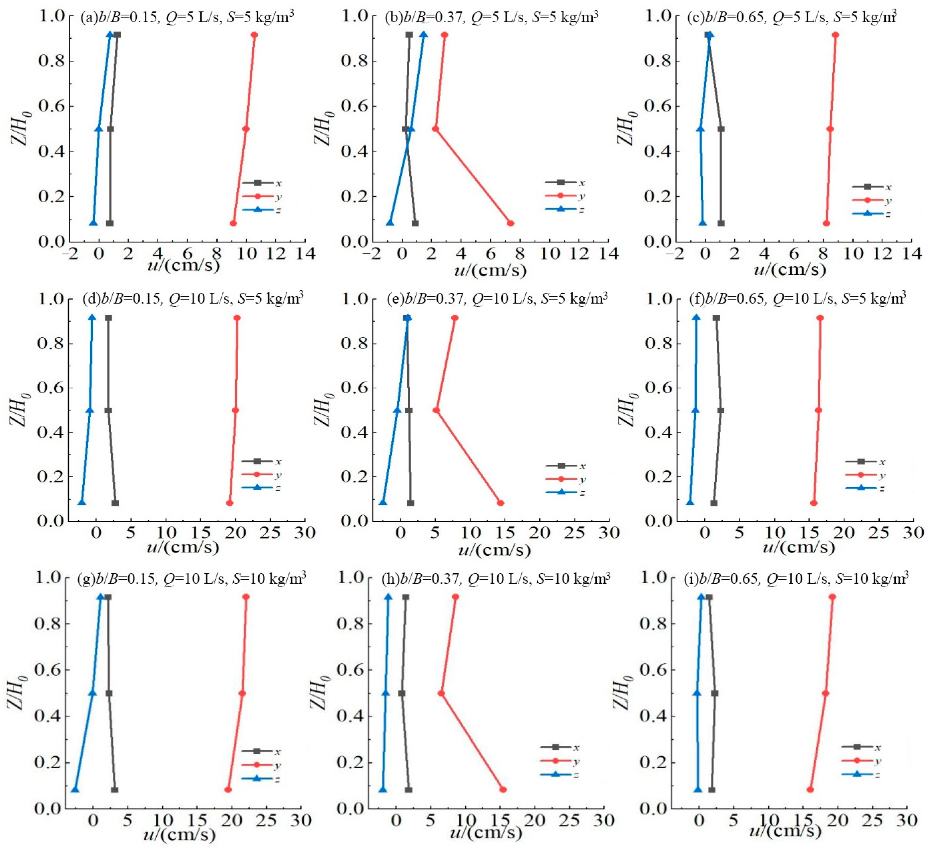
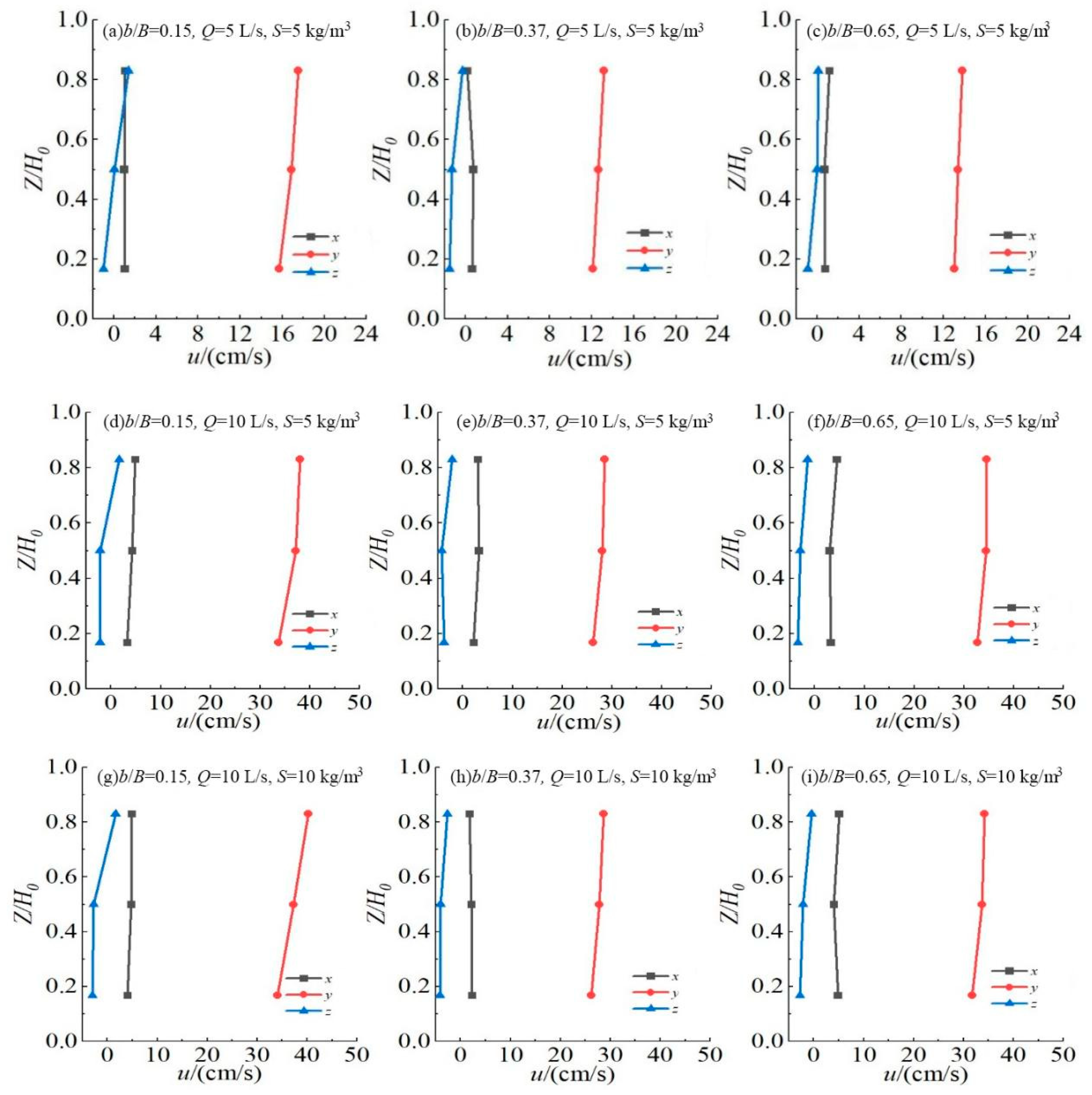
Based on experimental observations, the submergence process of the ecological protective forest can be divided into three distinct stages: trunk submergence stage, canopy submergence stage, and post-submergence stable stage. Based on the spatial distribution of mean velocity components, we infer the existence of complex flow patterns that may include trunk-scale turbulence and secondary circulation. These inferences are consistent with earlier vegetated-flow studies [2,15,16,25], but are not directly verified by turbulence measurements in the present experiment. Vegetation can slow down the flow velocity of water, a finding consistent with the research results of Khadami et al. [15]; Sediqi et al. [16]; and Xu et al. [17]. Vertical velocities in Regions I and III generally followed a logarithmic profile, and Region II exhibited a distinct velocity minimum within the canopy layer. In terms of sediment retention performance, arrangement A1 yielded the optimal deposition results, followed by A2 and A4, while A3 demonstrated the least effectiveness. Comparative analysis revealed that increased density of ecological protective forests generally enhances deposition thickness which agrees with the study of Sediqi et al. [16].

Horizontal vegetation density ρ_L emerged as a governing factor influencing deposition efficiency, as quantitatively detailed in

Table 4. Parameters of ρ_v and ρ_L for Q = 10 L/s and S = 5 kg/m³.

Arrangement	Submergence Degree H0/H = 0.5		Submergence Degree H0/H = 1.0
	ρv (%)	ρL (%)	ρv (%)	ρL (%)
A1	2.78	0.26	12.34	78.5
A2	2.78	0.21	12.34	62.8
A4	2.78	0.15	12.34	47.1
A3	1.67	0.15	7.41	47.1

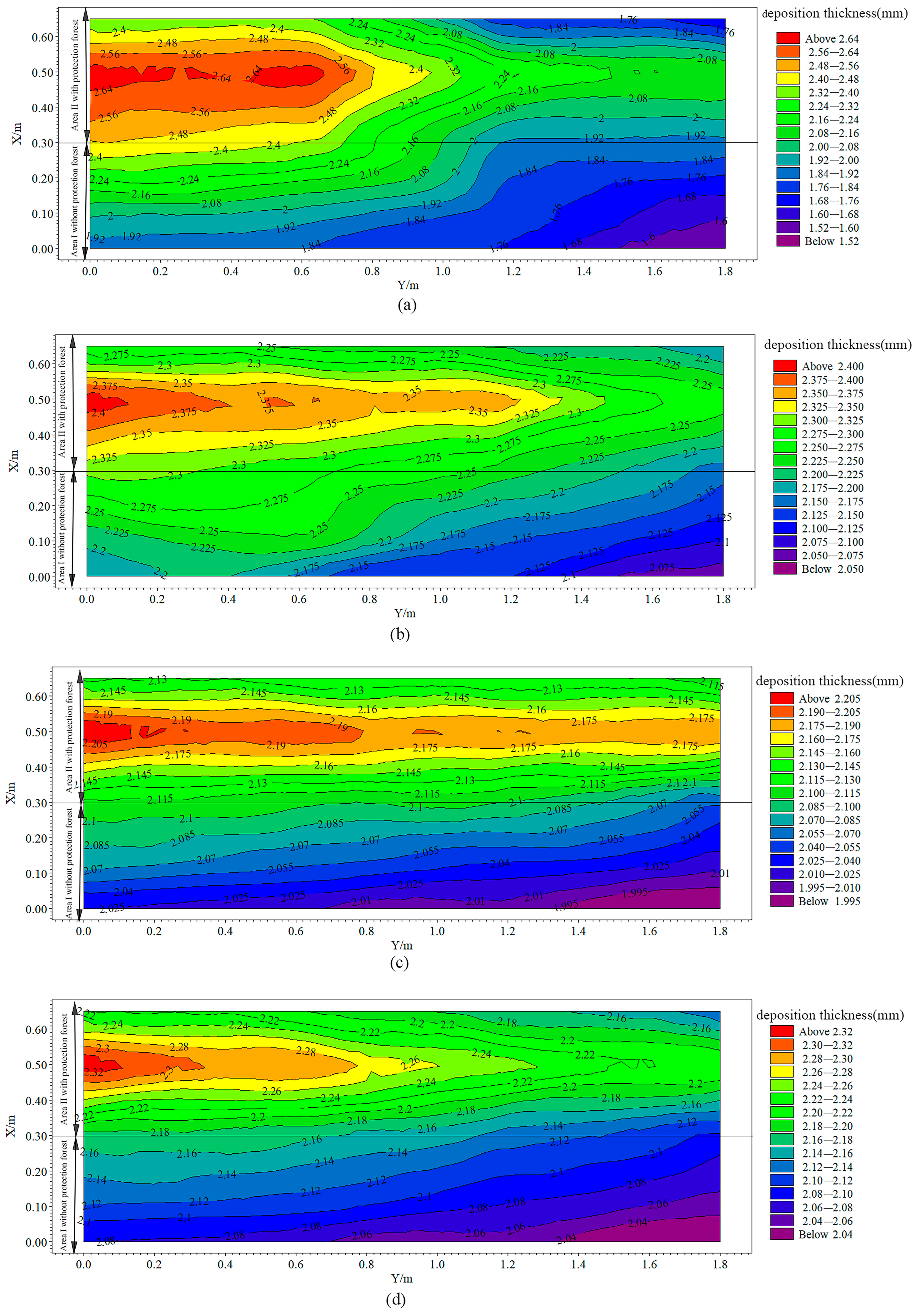
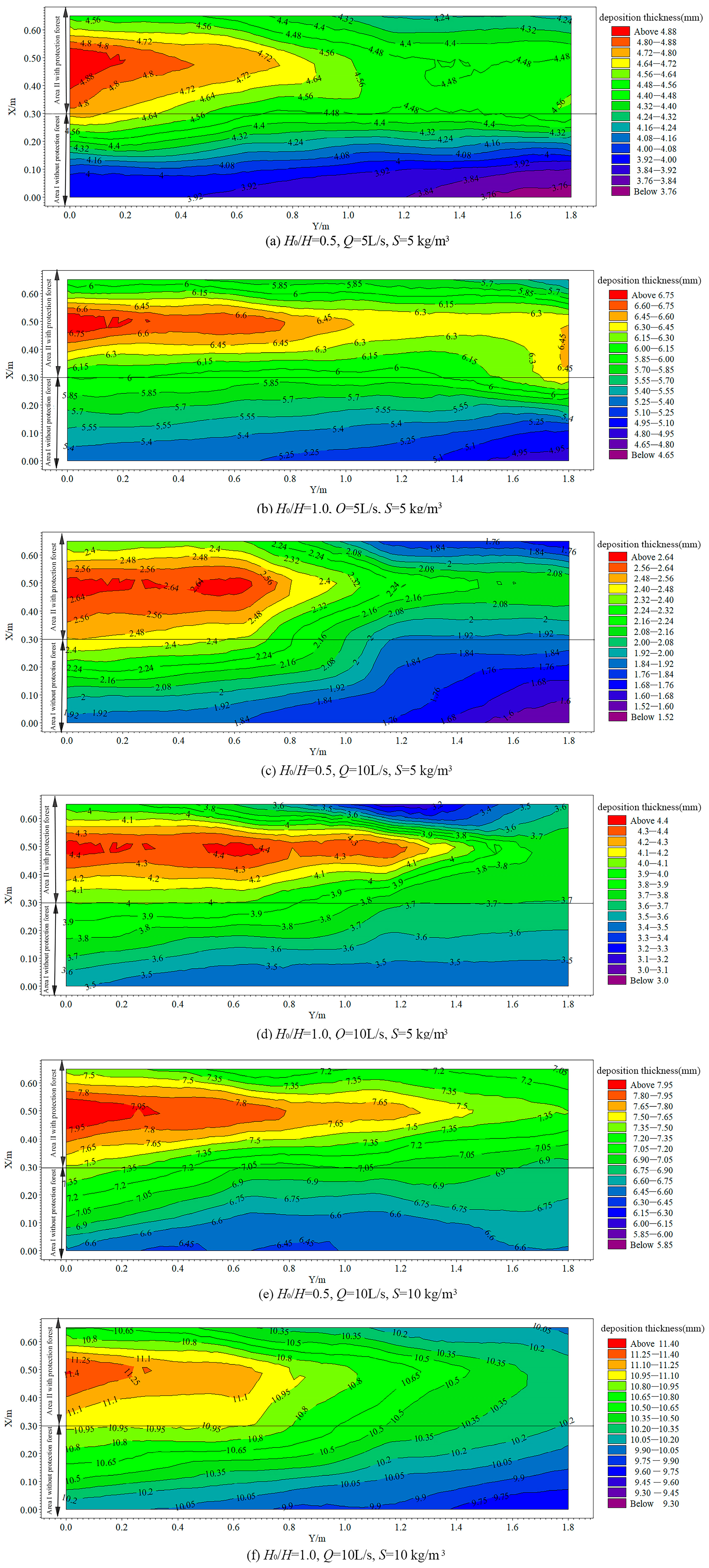
. Under identical horizontal vegetation density conditions, higher vertical vegetation density ρ_v consistently improved sediment retention capacity. The comparative relationship between the longitudinal and transverse spacing of trees determines the location of sediment deposition. An arrangement where the longitudinal spacing exceeds the transverse spacing can effectively promote sediment deposition.

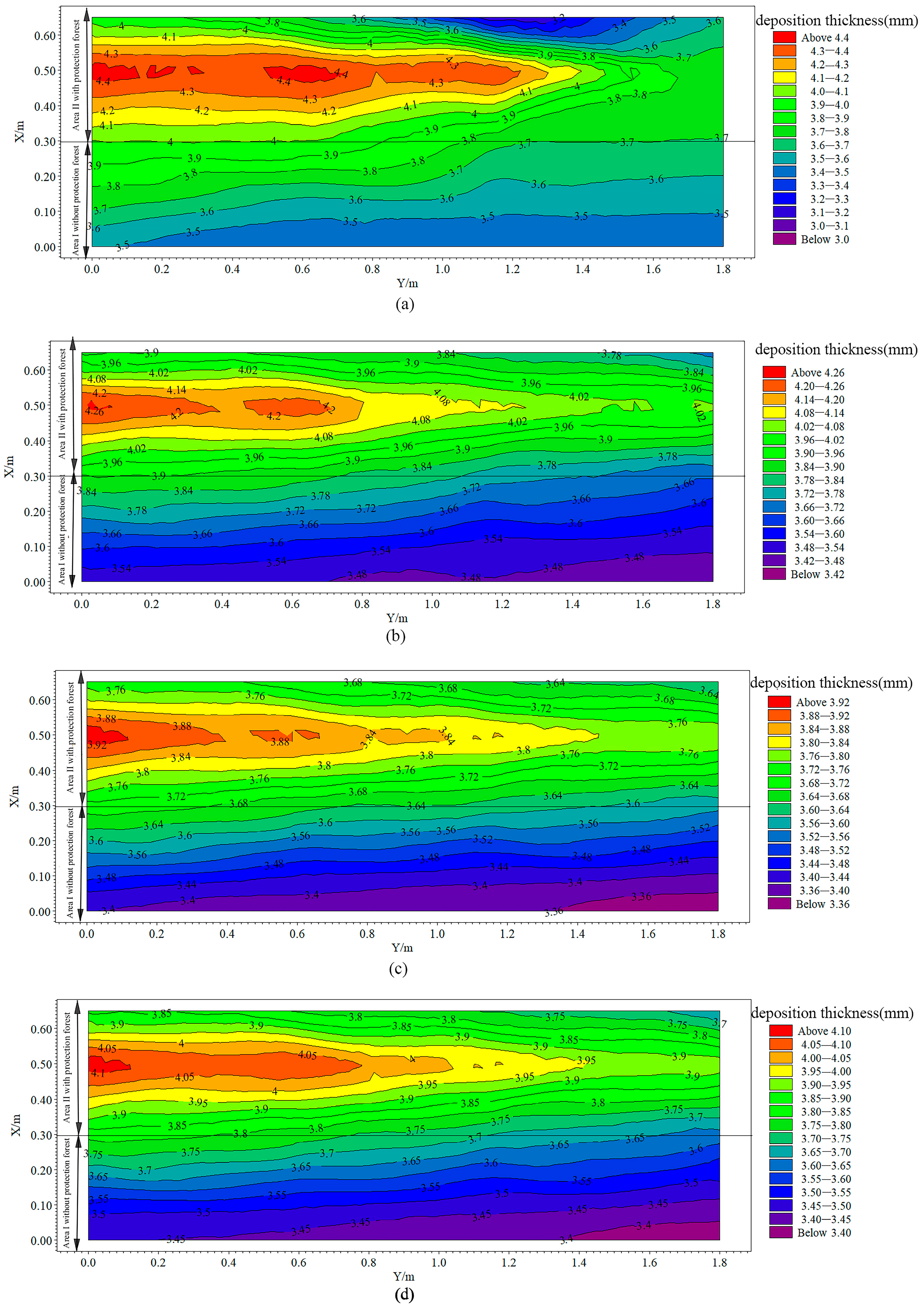
Additionally, we provide a qualitative comparison between our laboratory findings and available field observations from the lower Yellow River floodplain sites (Yuanyang, Changyuan, and Dongming), as cited in Ref. [7] and related surveys. Field observations at Dongming Beach indicate that sediment deposition is consistently thicker immediately upstream of existing protective forest patches than within or downstream. This matches our laboratory findings (Figure 8 and Figure 9), where the highest deposition occurred at CS1 (upstream of the forest leading edge) for all four arrangements. In the field, denser vegetation patches (naturally regenerated willow stands) show visibly greater sediment accumulation around trunks and along the toe of the embankment compared to sparser stands. Our A1 arrangement (highest vegetation density) consistently produced the greatest deposition thickness, confirming this monotonic relationship. 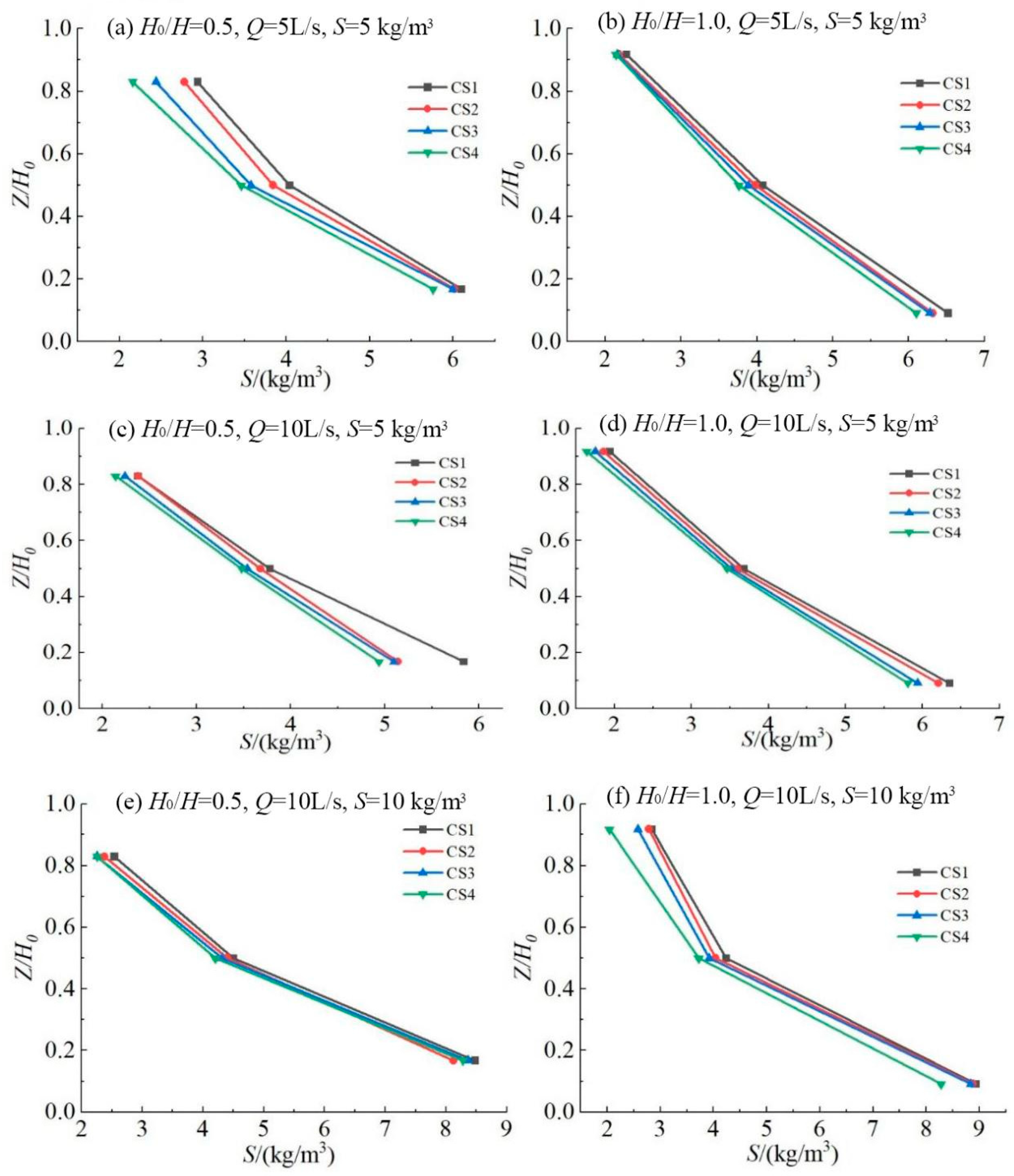Although high-resolution transect data are limited, concentration profiles measured at Yuanyang floodplain during moderate overbank events show a decreasing trend from the floodplain entrance towards the embankment toe, consistent with the longitudinal decay we quantified in Section 3.3.2 (Figure 12).

4.2. Further Discussion on Flow Incidence Angle

The experiments reported in this study were conducted exclusively under embankment-parallel flow conditions. As justified in Section 3.2, this configuration is hydrologically representative because floodplain inundation events in the lower Yellow River ultimately stabilize into prolonged flow parallel to the embankments. However, overbank flows initially often impinge obliquely on dike toes, and it is under such oblique or transverse incidence that flanking erosion can be most damaging. Therefore, it is important to discuss qualitatively how the ranking of arrangements (A1 > A2 > A4 > A3) might change under non-parallel flow conditions.

Under oblique or transverse flow incidence, the effective spacing between trees in the streamwise direction is no longer the original longitudinal (l_y) or transverse (l_x) spacing as defined in the flume coordinate system. Instead, the flow encounters a combination of both spacings depending on the incidence angle. For arrangement A1 (square grid, l_x = l_y = 7 cm), the geometry is isotropic: the frontal area presented to the flow is insensitive to incidence angle. Arrangement A3 (row spacing 14 cm in the transverse direction, 7 cm in the streamwise direction) and arrangement A4 (7 cm transverse, 14 cm streamwise) are highly anisotropic. Under oblique flow, A3 and A4 may behave more similarly because the effective spacings in the flow direction converge. In contrast, arrangement A2 (alternating wide and narrow spacings in both directions) may create local flow acceleration and deceleration patterns that are sensitive to incidence angle. The relative superiority of A1 is likely to be robust. The ranking between A3 and A4 may become less distinct or even reverse under highly oblique or transverse flow, because their anisotropic spacing geometries exchange roles as the flow direction changes. A2 may experience a more complex response, potentially reducing its deposition effectiveness relative to A1, because alternating wide and narrow gaps could cause flow channeling under oblique incidence.

Thus, while the present results provide a clear ranking for embankment-parallel flow, the practical recommendation for field implementation (A1 with a row-to-plant spacing ratio of 1.0) should be considered robust only for the dominant flow direction parallel to the embankment. For sites where oblique or transverse overbank flows are frequent and erosive, additional experimental or numerical studies are needed to evaluate the performance of anisotropic arrangements (A2, A3, A4) under varying incidence angles. The present study therefore serves as a baseline, and future work should extend the investigation to oblique flow conditions.

4.3. Limitations

We selected a geometric scale to establish a flume experiment by scaling down the natural river channel and ecological protective forests accordingly. To better align the experimental conditions with natural flow characteristics, additional similarity criteria were considered, such as gravitational similarity, flow resistance similarity, and sediment movement similarity. It should be noted that due to the sediment particle size in the lower Yellow River being less than 1 mm, it was impossible to scale down the sediment according to the corresponding ratio. Therefore, natural sand (with a measured median diameter d₅₀ = 0.0255 mm) was used in the experiment. This resulted in dissimilarities between the experimentally measured flow velocity and sediment deposition thickness and those under natural conditions, making it impossible to directly scale the experimental data to represent natural river parameters. Given the complex nature of sediment-related issues in rivers, obtaining precise quantitative data is challenging, a limitation also observed in previous studies [40,41,42,43,44]. This represents a constraint of the present study. Nevertheless, the regular patterns observed in the experiment can still provide scientific reference for disaster mitigation and flood control in the lower Yellow River.

(1) Direction of bias

Using unscaled natural fines (instead of lighter or coarser scaled sediment) likely leads to an underestimation of the deposition-promotion percentages reported in this study. The present fine sediment remains suspended longer, requiring greater flow deceleration to settle. Consequently, the measured promotion percentages (e.g., 6.8–20.6% for arrangement A1) are conservative lower-bound estimates. Conversely, the velocity reduction caused by vegetation is less affected by sediment scaling, because it is governed primarily by geometric and hydraulic similarity (Froude and Reynolds constraints), which were satisfied.

(2) Robustness of data

The relative ordering of sediment deposition effectiveness (A1 > A2 > A4 > A3) is robust and can be confidently transferred to prototype conditions. This ranking is governed by the row-to-plant spacing ratio and the resulting flow-blocking geometry, which are correctly represented even with unscaled sediment because all arrangements experienced the same sediment-scaling bias. In contrast, the absolute percentage values should be treated as qualitative indicators of relative performance rather than precise design numbers for the prototype Yellow River. The magnitudes are influenced by the unscaled sediment and should not be directly extrapolated without site-specific calibration.

(3) Guidance for transfer to prototype conditions

Advised to use the reported percentages only for comparative ranking among arrangements (A1 > A2 > A4 > A3) and for understanding the influence of submergence degree and spacing ratio. For quantitative design of ecological protective forests along the lower Yellow River embankments, the following conservative approach is recommended: (i) adopt the relative performance order to select arrangement A1 as the preferred layout; (ii) apply the measured promotion percentages as a lower-bound estimate; (iii) perform field validation or numerical modeling (e.g., using a calibrated vegetation drag model) to obtain site-specific deposition rates, because the absolute values cannot be obtained by simple geometric scaling of the flume data. The key transferable insight is that maximum horizontal vegetation density ρ_L and a row-to-plant spacing ratio of 1.0 (arrangement A1) maximizes deposition efficiency, not the specific percentage numbers.

Additionally, this study reports only mean velocity components measured with an electromagnetic current meter. No measurements of fluctuating velocities were obtained, such as Reynolds stresses, turbulent kinetic energy, or eddy frequencies. Therefore, interpretations involving wake turbulence, vortex shedding, or secondary circulation are qualitative inferences drawn from the existing literature rather than direct experimental evidence. Future work should employ advanced instrumentation (e.g., Acoustic Doppler Velocimeter, Particle Image Velocimetry) to directly quantify turbulence dynamics in ecological protective forests. Furthermore, this study does not consider non-rigid vegetation or the combined effects of waves and currents. As discussed in Section 2.3.2, the use of rigid vegetation models instead of flexible ones introduces a systematic bias. Based on the literature on flexible vegetation reconfiguration [37,38,39], rigid models overestimate drag forces by an amount that depends on flow velocity, vegetation stiffness, and submergence degree. Under fully submerged conditions with high flow velocities, the overestimation can be substantial. Consequently, the sediment deposition promotion percentages reported in this study (e.g., 6.8–20.6% for arrangement A1) likely represent upper-bound estimates for the performance of actual flexible protective forests under similar flow conditions. Future research should introduce a flexible vegetation model to verify the generalizability of the current research.

4.4. Practical Implications for Embankment Management

The present experiments demonstrate that arrangement A1 is the most effective among the four tested configurations for promoting sediment deposition under embankment-parallel flow conditions. However, translating this laboratory ranking into operational design choices for the Yellow River Conservancy Commission requires consideration of several practical constraints.

Arrangement A1 has the highest stem density per unit area. In many reaches of the lower Yellow River, the space between the embankment toe and the edge of the floodplain is limited by existing infrastructure such as roads, drainage ditches, and agricultural fields. Where land width is narrow, A1 may be physically impossible to implement at full scale. In such cases, A2 or A4 (which retain the same transverse spacing but reduce longitudinal density) could serve as practical compromises, acknowledging that they provide lower deposition enhancement (A2 and A4 gave 5.4% and 5.4% promotion under semi-submerged conditions vs. 7.6% for A1).

A1 requires approximately twice as many trees per hectare as A3 or A4, and roughly 1.5 times as many as A2 (depending on the exact removal pattern). For long embankment sections (hundreds of kilometers), the additional cost of seedlings, labor for planting, and subsequent maintenance (pruning, disease control, flood-damage replacement) is non-negligible. A cost-effectiveness analysis, balancing deposition benefit against planting density, would be needed before large-scale adoption.

A1 approximates a monoculture-like, high-density plantation. Continuous dense stands of a single tree species (e.g., willow or ash) may reduce habitat heterogeneity compared to patchier arrangements (A2 or A3) or mixed-species designs. While biodiversity was not an endpoint of this study, river managers are increasingly required to consider ecological co-benefits. A mosaic of A1 patches in high-priority erosion zones interspersed with lower-density A2 or A4 patches elsewhere might balance hydraulic performance with habitat diversity.

Dense forests reduce flow velocity effectively, which is desirable for deposition but may also back up floodwaters upstream, potentially increasing water levels and levee overtopping risk elsewhere. During extreme floods, rigid dense arrangements (A1) are more likely to trap woody debris, agricultural waste, or ice, which can further obstruct flow and cause local scour around accumulated material. The present experiments did not include debris or extreme flood conditions; therefore, the ranking A1 > A2 > A4 > A3 should be considered valid for ordinary overbank flows but not automatically extrapolated to design-flood conditions without additional study.

In summary, while arrangement A1 offers the highest deposition-promotion potential, its practical superiority must be weighed against land availability, cost, biodiversity, and extreme-flow conveyance. The most resilient solution for the lower Yellow River embankments is likely a context-dependent, multi-arrangement strategy rather than a single, uniform layout.

5. Conclusions

Based on field investigations of ecological protective forests in the lower Yellow River, an experimental flume was designed following similarity principles, with forest models constructed to represent typical morphological characteristics. A series of experiments was conducted under varied water–sediment conditions and abnormal flow scenarios. The flow-reducing and promoting sediment deposition effects of different arrangements, hydrological combinations, and submergence states were systematically analyzed. For the optimal arrangement pattern, detailed flow velocity and sediment concentration distributions were examined. Based on these findings, we discuss practical implementation considerations for the Yellow River Conservancy Commission. The main findings are summarized as follows:

(1) For high flow with low-sediment conditions with embankment-parallel flow, the average sediment deposition promotion rates for arrangements A1 to A4 were 7.6%, 5.4%, 4.7%, and 5.4%, respectively, under semi-submerged conditions. At full submerged state, the corresponding values increased to 11.38%, 10.85%, 8.60%, and 10.34%. Sediment promoted deposition efficiency increases with vegetation density and A1 providing the strongest promotion of deposition. For a given density, configurations with greater concentration in the transverse (x) direction yield superior deposition performance. Arrangement A1 is recommended as the priority layout for actual embankment engineering projects, with a maximum horizontal vegetation density ρ_L and a row-to-plant spacing ratio of 1.0.

(2) The flow-reducing effect of riverside ecological protective forests typically ranges between 5% and 75%, with particularly significant velocity reduction (up to 75%) observed at the relative depth Z/H₀ = 0.5 under full submergence. Vertically, the streamwise velocity profile in semi-submerged forests (H₀/H = 0.5) maintains a similar J-shaped distribution, while full submergence (H₀/H = 1.0) produces a distinct velocity minimum near the canopy base.

(3) Across all experimental scenarios and regardless of submergence condition, the ecological protective forest area consistently exhibited a characteristic vertical sediment distribution: minimum concentrations near the water surface and maximum concentrations near the bed. At full submergence (H₀/H = 1.0), the vertical gradients of both surface and mid-depth sediment concentration profiles were notably steeper than those observed at semi-submerged state (H₀/H = 0.5), indicating significant canopy-induced modification of sediment distribution patterns in the water column. Furthermore, a clear longitudinal attenuation in sediment concentration was observed along the flow path through the forested area.