Article

Quantifying Non-Fickian Pollutant Transport in Layered Heterogeneous Media Under Non-Uniform Flow Field: Bimodal Transport and Sub-Diffusion


1
School of Architecture and Civil Engineering, Anhui Polytechnic University, Wuhu 241000, China
2
State Key Laboratory of Water Disaster Prevention, Nanjing 210098, China
3
School of Chemistry and Materials Science, University of Science and Technology of China, Hefei 230026, China
*
Authors to whom correspondence should be addressed.
Water 2026, 18(11), 1309; https://doi.org/10.3390/w18111309
Submission received: 15 April 2026 / Revised: 24 May 2026 / Accepted: 26 May 2026 / Published: 28 May 2026
(This article belongs to the Special Issue Fate and Transport of Contaminants in Soil and Water)

Abstract

Characterizing pollutant transport in heterogeneous layered media, such as structured surface soils and layered aquifers, is crucial for predicting and managing environmental pollution. However, the characterization of the coupled bimodal transport and sub-diffusion dynamics of contaminants in layered porous media under a non-uniform flow field remains challenging. In this paper, we develop a 2D-fractional multi-peak (2D-FMP) model to systematically investigate the complicated non-Fickian pollutant transport in the layered media systems. The model analysis reveals the effects of hydrological properties and media heterogeneity on bimodal transport and sub-diffusion behavior. The results show that: (1) The two-peak pollutant transport behavior becomes more apparent as the contrast in media porosity increases. Furthermore, an increase in dispersivity within the slow region (region 1) decreases the concentration value of the second peak in the entire region, indicating that discrepancies in media properties are critical factors influencing multi-peak transport. (2) A smaller time index in region 1 ( γ 1 ) results in a lower concentration value for the second peak across the entire region, and the power-law late-time tails become heavier as γ 1 decreases. This indicates that discrepancies in media heterogeneity between region 1 and region 2 also significantly influence anomalous bimodal transport. The model’s application further validates the ability of the 2D-FMP framework to capture coupled bimodal transport and sub-diffusion in natural layered media. The 2D-FMP model developed in this study sheds light on the quantification of non-Fickian transport in layered media systems.

1. Introduction

Layered media are ubiquitous in surface and subsurface environments, such as structured surface soil [1,2,3], fractured formations [4,5,6], and aquifer–aquitard systems [7,8,9]. Pollutants released in layered media usually exhibit anomalous transport behavior characterized by late-time tails (sub-diffusion) [10,11,12,13] or early leading edges (super-diffusion) [14]. Field and laboratory experiments have revealed that solute transport in layered heterogeneous media may also show apparent multi-peak characteristics [15,16,17,18,19]. It is generally accepted that non-Fickian solute transport in layered media is caused by media heterogeneity [20], while multi-peak transport is attributed to the layered media’s structure [17]. The traditional one-dimensional advection–dispersion equation (ADE) cannot capture either the non-Fickian transport behavior or the multi-peak transport in heterogeneous media, motivating the development and application of non-local models and dual-region models.
Previous research focused on investigating the multi-peak transport behavior observed during field experiments in structured formations. For example, Coats and Smith proposed a double-domain model to capture solute transport in layered fractured media, where the structured media are divided into mobile and immobile regions [21]. Skopp et al. derived a dual-permeability model for solute transport in dual-permeable regions, where a series of advection–dispersion equations are used for different regions [22]. Field and Leij successfully applied the dual-domain advection–dispersion equations (DADEs) to describe the multiple peaks of breakthrough curves (BTCs) observed in laboratory dual conduit tracer experiments [23]. Wang et al. investigated dual-peaked BTCs in a karst tracer test using the same DADE model [24]. Most of the conceptual models utilize the Fickian theory to describe the solute transport in each domain of the layered media and ignore the local media heterogeneity in both layered regions. However, the media heterogeneity and/or pollutant adsorption are critical factors influencing contaminant transport in natural porous media, invariably resulting in non-Fickian transport behavior [25]. Thus, accounting for the effects of the media heterogeneity and pollutant adsorption is essential for accurately characterizing the pollutant transport dynamics in the layered media systems.
To capture the anomalous, non-Fickian transport behavior of solutes, several promising stochastic and non-local methods have been developed. The multi-rate mass transfer (MRMT) model [26,27], extended from mobile–immobile concepts, is widely used due to its clear hydrological meaning; it divides the heterogeneous media into one dominant mobile region and a series of immobile regions where mass exchange retards solute transport, resulting in sub-diffusion. Another powerful approach is the continuous time random walk (CTRW) framework [28,29,30], an upscaling stochastic model that defines the distribution for transition times between solute particle jumps, leading to various memory functions for complex non-Fickian dynamics. Furthermore, fractional derivative models, such as the time-fractional advection–dispersion equation (T-FADE) [31,32,33,34] offer parsimonious representations of non-Fickian transport, capturing sub-diffusion due to trapping [35,36,37]. Distributed-order fractional models further extend this by utilizing a distribution of fractional derivative orders to capture complex, time-varying memory effects [38]. A detailed description of the relationship between MRMT, CTRW, and T-FADE can be found in Dentz and Berkowitz (2003) [35].
Despite the success, the above models suffer from critical limitations when applied to layered heterogeneous systems under realistic hydraulic conditions. Specifically, two major limitations remain unaddressed by current frameworks. First, there is a persistent inability to simultaneously capture bimodal behavior and anomalous diffusion. Standard non-local models (including MRMT, CTRW) are fundamentally single-domain or mobile–immobile frameworks designed for a single dominant mobile pathway. Consequently, they cannot resolve the multi-peak BTCs stemming from parallel, competing mobile pathways with highly contrasting velocities. Conversely, classical dual-domain models (like the DADE) successfully replicate multi-peak behaviors but enforce local Fickian transport, thereby failing to capture the non-Fickian heavy tails arising from sub-grid micro-heterogeneity within each individual layer. Second, existing fractional multi-peak models neglect scale-dependent, non-uniform velocity fields. In practical applications like radial divergent or convergent tracer tests, solute particles experience non-uniform flow fields where both the average pore velocity and the hydrodynamic dispersion coefficient are scale-dependent [39,40,41,42,43]. It remains poorly understood how this spatial non-uniformity couples with local sub-grid heterogeneity to govern bimodal, non-Fickian transport dynamics.
To address these limitations, this study develops a two-domain fractional multi-peak (2D-FMP) model. The principal methodological innovations of this work are twofold: (1) We expand the utility of fractional derivative models to capture non-Fickian transport in layered media by mathematically incorporating scale-dependent, non-uniform velocity and dispersion fields. (2) The proposed 2D-FMP model innovates by coupling two parallel pathways via a dynamic mass-exchange term. This dual-mobile fractional structure enables the simultaneous modeling of bimodal transport and sub-diffusion under non-uniform flow domains.
This study aims to characterize bimodal, non-Fickian transport behavior of pollutants in layered media under non-uniform velocity conditions. We develop the 2D-FMP model based on fractional theory to capture these complex transport dynamics. The model is then solved numerically, and its accuracy is validated against existing analytical and numerical solutions. Finally, we systematically investigate the coupled effects of media property discrepancies, sub-grid heterogeneity, and scale-dependent flow parameters on solute transport.

2. Concept and Mathematic Model

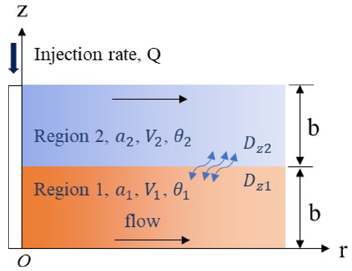
The schematic of pollutant transport in an infinite two-dimensional layered media with non-uniform flow distribution is presented in Figure 1. Several simplifying assumptions underlie the development of the proposed 2D-FMP model. First, the geological system is idealized as a two-layer formation with macroscopically uniform and constant thickness b (consistent for both the upper and lower regions), neglecting minor undulating boundaries common in natural stratigraphy. Both regions are assumed to be heterogeneous, with different porosities and dispersivities. Second, the flow fields within both layers are assumed to have reached a steady state, meaning that the pore velocity depends solely on radial distance r while micro-scale vertical velocity components across the interface are ignored. Solute transport in both regions is assumed to be dominated by advection and dispersion along the radial direction, together with dispersion along the z-axis. Third, mass transfer across the layer interface is assumed to be driven strictly by Fickian-like vertical dispersion (i.e., diffusion along the z-axis). Moreover, following Zhou et al., the retention and adsorption of solute in porous media follow a power-law distribution (see mathematical derivation in Section S1) [14,33,44,45,46]; accordingly, these processes in both regions are captured by the fractional derivative operator employed in this work. A tracer with a concentration C 0 is injected into the injection well at a constant flow rate Q after the flow field has reached steady state, and a zero initial concentration is set for the entire layered media.
Pollutant transport in the radial layered heterogeneous media can thus be described by the following 2D-fractional multi-peak (2D-FMP) model:
C 1 t + β 1 γ 1 C 1 t γ 1 = V 1 C 1 r + 1 r r r D x 1 C 1 r + D z 1 2 C 1 z 2 ,
C 2 t + β 2 γ 2 C 2 t γ 2 = V 2 C 2 r + 1 r r r D x 2 C 2 r + D z 2 2 C 2 z 2 .
The initial and boundary conditions take the following form:
C 1 r , z , 0 = C 2 r , z , 0 = 0 ,
C 1 r = 0 , z , t = C 2 r = 0 , z , t = C 0 ,
C 1 ( r = , z , t ) r = 0 ,
C 2 ( r = , z , t ) r = 0 .
The interface boundary conditions between region 1 and region 2 are defined as:
C 1 r , z = b , t = C 2 r , z = b , t ,
θ 1 D z 1 C 1 ( r , z , t ) z   z = b = θ 2 D z 2 C 2 ( r , z , t ) z   z = b ,
where the subscripts 1 and 2 represent region 1 and region 2, respectively. C [ML−3] is the concentration of solute in the layered media. γ t γ is the Caputo fractional derivative operator with 0 < γ 1 . β [ T γ 1 ] is the fractional capacity coefficient representing the ratio between the immobile and mobile region. γ [−] is the time index, representing the heterogeneity of the media. b [L] is the layer thickness, V [LT−1] is the radial velocity, D x [L2T−1] and D z [L2T−1] are the longitudinal dispersion coefficient in the radial direction and diffusion coefficients in the z direction, respectively, and θ [−] is the porosity of the region. It should be noted that both β and the time index γ govern the retention and sorption processes of pollutants. A smaller γ or a larger β results in a heavier sub-diffusion of the pollutant in the porous media.
The steady-state velocity in the two regions can be expressed as:
V 1 = Q 2 π θ 1 b r ,
V 2 = Q 2 π θ 2 b r .
where Q [M3T−1] is the injection flow rate.
The radial dispersion coefficient can be expressed as:
D x 1 = a 1 V 1 + D 0 ,
D x 2 = a 2 V 2 + D 0 ,
where a 1 [M] and a 2 [M] are the dispersivities in region 1 and region 2, respectively. D 0 [L2T−1] is the molecular diffusion coefficient, which is neglected in our work.
Therefore, the governing equations (Equations (1) and (2)) can be rearranged as:
C 1 t + β 1 γ 1 C 1 t γ 1 = k 1 r C 1 r + k 1 a 1 r 2 C 1 r 2 + D z 1 2 C 1 z 2 ,
C 2 t + β 2 γ 2 C 2 t γ 2 = k 2 r C 2 r + k 2 a 2 r 2 C 2 r 2 + D z 2 2 C 2 z 2 ,
where k 1 = Q 2 π θ 1 b and k 2 = Q 2 π θ 2 b .

3. Methodology

3.1. Discretization of the Governing Equation Using the Finite Volume Method

Due to the non-linearity of the coupled equations, obtaining the analytical or the semi-analytical solution of the 2D-FMP is challenging. In this paper, we applied the finite volume method to numerically solve the two-dimensional problem. A detailed description of the numerical convergence verification, stability considerations, sensitivity of the numerical solution to discretization parameters, and additional information regarding implementation of the fractional derivative operator can be found in the Supplementary Materials (See Section S2) [47,48].
The general cylindrical governing equation for solute transport in two-dimensional layered media can be given as:
C t + β γ C t γ = k r C r + k a r 2 C r 2 + D 2 C z 2 ,
The discretization of the equation in the control volume P and at the time domain t , t + t can be written as:
Δ z Δ r Δ t ( C p j + 1 C P j ) + β Δ z Δ r Δ t γ Γ ( 2 γ ) ( C p j + 1 C P j ) = 1 r p ( k e C e j + 1 k w C w j + 1 ) Δ z + 1 r p ( k a C j + 1 r e k a C j + 1 r w ) Δ z + ( D C j + 1 z n D C j + 1 z s ) Δ r Δ z Δ r m = 1 j C p j m + 1 C p j m Δ t ( m + 1 ) 1 γ m 1 γ
where r P is the distance from point P to the inlet. Rearranging Equation (16), we obtain:
A P C P j + 1 = A E C E j + 1 + A W C W j + 1 + A N C N j + 1 + A S C S j + 1 + S P C P j + S u e r r o r ,
where
A P = z r t + β z r t γ Γ ( 2 γ ) + A E + A W + A N + A S + Δ F S P , A E = z k e 2 r P + z k e a e r p δ x P E ,   A W = z k w 2 r P + z k w a w r p δ x P W ,   A N = r D n δ x P N ,   A S = r D s δ x P S ,   F = z k e r P z k w r P , e r r o r = z r m = 1 j C P j m + 1 C P j m t m + 1 1 γ m 1 γ .
The dispersivity ( a ) at the interface can be calculated using the arithmetic mean method or upwind mean method [49].

3.2. Initial and Boundary Condition

A first-type boundary condition with a constant concentration C 0 and a zero gradient boundary condition are applied at the inlet and outlet of the layered media system, respectively. A zero initial condition is used for the entire porous media domain. Consequently, Equation (17) at the inlet can be written as:
A P C P j + 1 = A E C E j + 1 + A W C W j + 1 + A N C N j + 1 + A S C S j + 1 + S P C P j + S u e r r o r ,  
where
A P = z r t + β z r t γ Γ ( 2 γ ) + A E + A W + A N + A S + Δ F S P .   A E = z k e 2 r P + z k e a e r p δ x P E ,   A W = 0 ,   A N = r D n δ x P N ,   A S = r D s δ x P S ,   F = z k e r P z k w r P   S P = z k w r P 2 z k w a w r p δ x P W ,   S u = ( z k w r P + z k w a w r p δ x P W ) C 0   e r r o r = z r m = 1 j C P j m + 1 C P j m t m + 1 1 γ m 1 γ .

3.3. Velocity-Averaged Solute Concentration

As reported by Liang et al., the solute concentration in the layered media at a fixed position r can be expressed as the velocity-averaged concentration along the z direction, which physically represents the mass of solute crossing a control plane per unit time. The velocity-averaged concentration for region 1, region 2, and the total region takes the following forms [50]:
C a v e 1 = b 2 b θ 1 C 1 V 1 d z b 2 b θ 1 V 1 d z ,
C a v e 2 = 0 b θ 2 C 2 V 2 d z 0 b θ 2 V 2 d z ,
C t o t a l = b 2 b θ 1 C 1 V 1 d z + 0 b θ 2 C 2 V 2 d z b 2 b θ 1 V 1 d z + 0 b θ 2 V 2 d z ,
where C 1 and C 2 are calculated from the above numerical solutions (Equations (15)–(18)). C a v e 1 is the velocity-averaged concentration for region 1, C a v e 2 is the velocity-averaged concentration for region 2, and C t o t a l is the velocity-averaged concentration for the total region. In the following sections, all analyses are performed using the normalized concentration C n o r m = C / C 0 .

3.4. Solution Validation

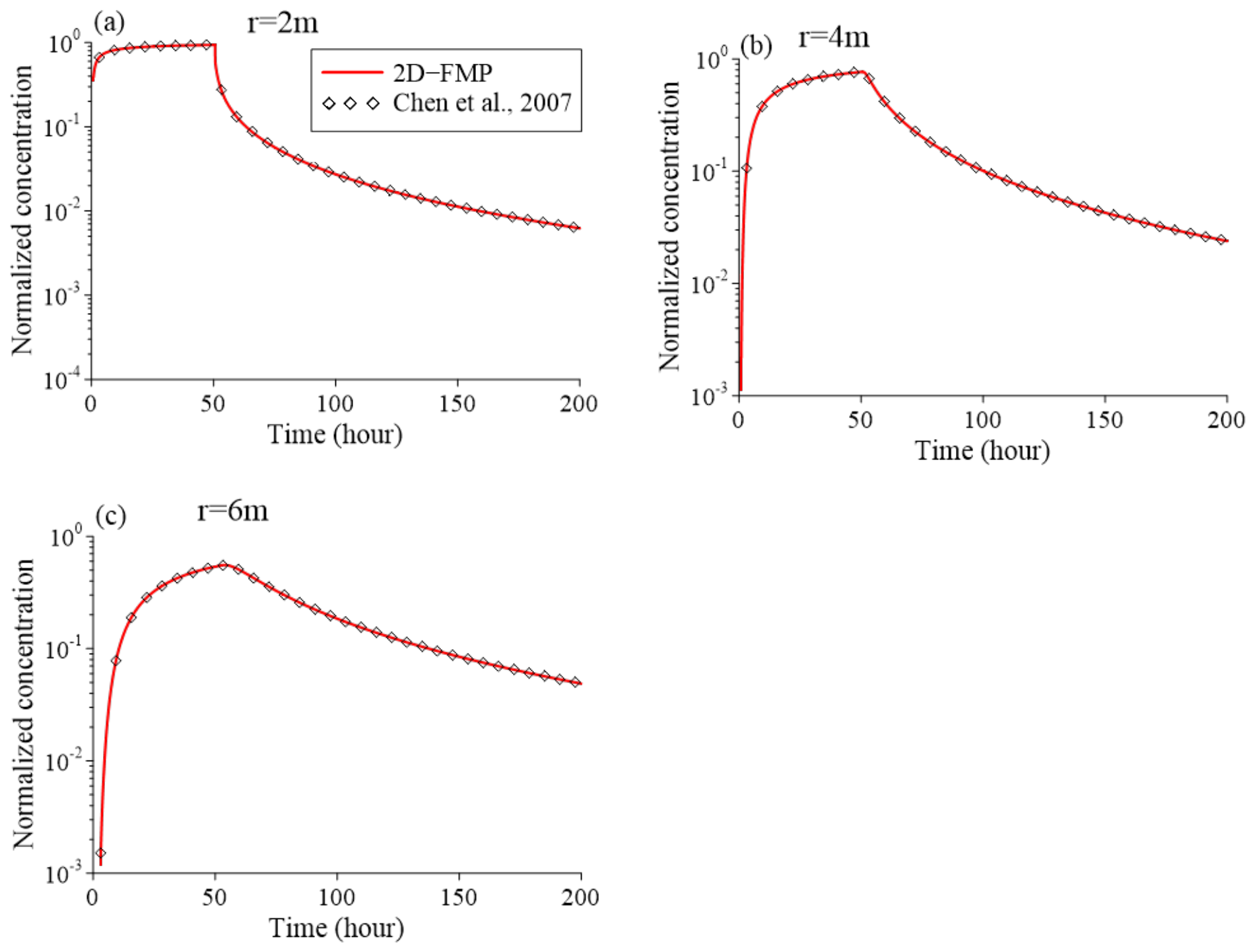
We adopted a semi-analytical solution proposed by Chen et al. (2007) to validate the numerical solution of 2D-FMP model [39]. The model proposed by Chen et al. (2007) can be considered as a special case of the 2D-FMP model in which the layered regions possess identical properties (the same dispersivity and porosity), the transverse diffusion between the layered regions is set to be zero, and solute retention in the heterogeneous media is neglected ( β = 0) [39]. As is shown in Figure 2, the numerical solutions of the 2D-FMP model at different positions (r = 2, 4, 6) are consistent with the results generated by the semi-analytical solution in Chen et al. (2007), demonstrating the accuracy of the finite volume method in solving 2D-FMP equations [39].

3.5. Sensitivity Analysis

We performed a local sensitivity analysis to systematically assess the response of simulated solute concentrations to variations in key model parameters, including porosity θ 1 , dispersivity a 1 , and the fractional derivative index γ 1 . To enable a fair comparison across parameters with different physical units, a dimensionless normalized sensitivity coefficient S j ( t ) was introduced:
S j t = C t P j P j C t ,
where C ( t ) is the simulated velocity-averaged concentration at time t , and P j is the j -th parameter. Because directly differentiating the time-fractional model equations analytically is highly challenging, the partial derivative was numerically approximated using a second-order accurate central finite-difference scheme:
C ( t ) P j C t ; P j + Δ P j C t ; P j Δ P j 2 Δ P j ,
The perturbation Δ P j was set proportional to the nominal parameter value, specifically Δ P j = 1 0 3 P j to balance numerical precision and avoid round-off errors.
The sign of the normalized sensitivity coefficient provides direct physical insight: a positive value ( S j t > 0 ) indicates that the concentration increases with the parameter, a negative value ( S j t < 0 ) indicates an inverse relationship, and a zero value implies insensitivity at that time. By plotting S j t over the entire breakthrough curve, one can identify which transport stages (e.g., early advective sweep, bimodal peak transition, or late-time sub-diffusive tailing) are dominated by which physical process.

4. Results and Discussion

4.1. Effects of Porosity and Dispersivity on Anomalous Bimodal Transport in Layered Media

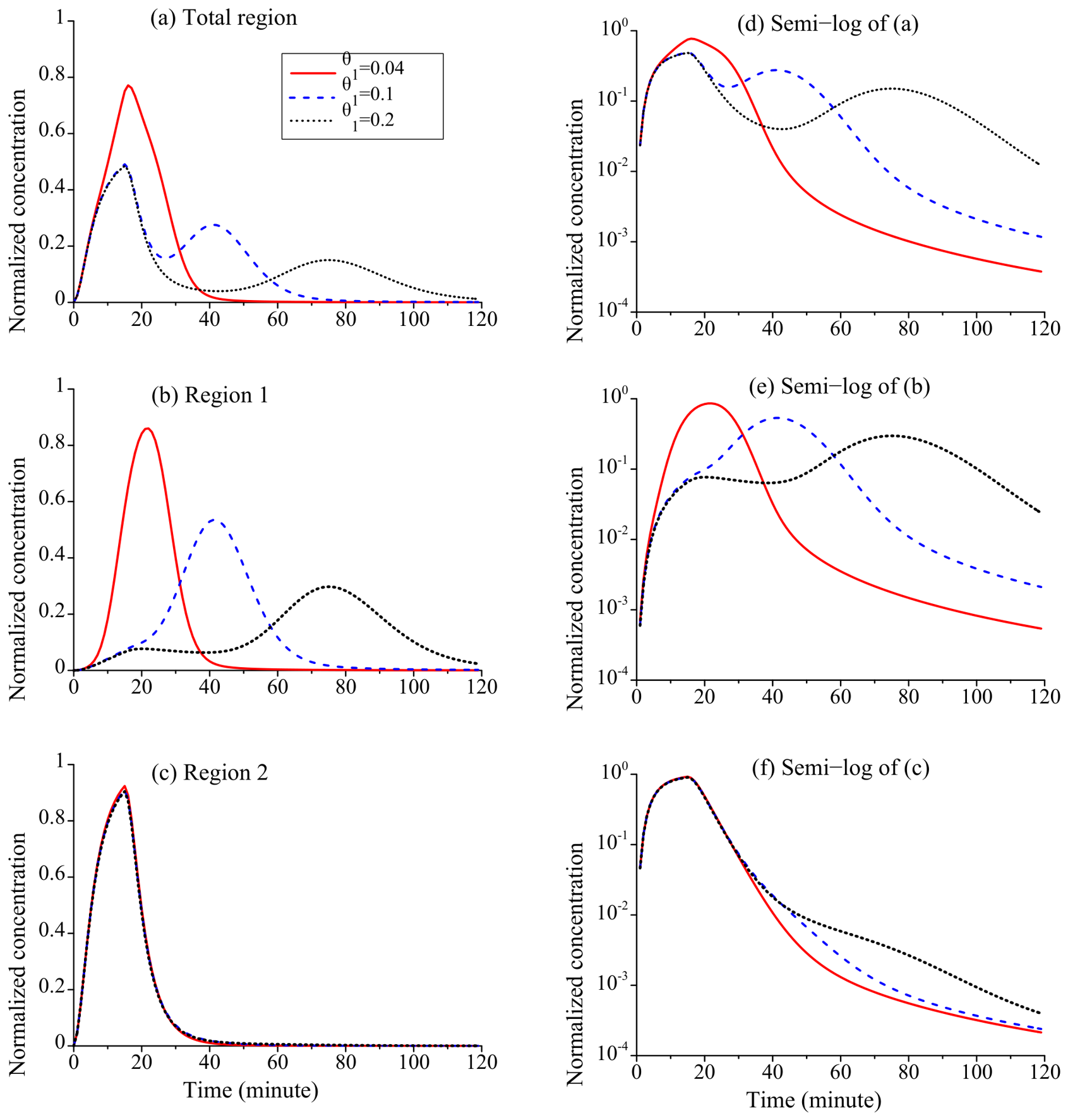
We first investigate the impacts of scale-dependent flow velocity and hydraulic dispersion governed by media porosity ( θ ) and dispersivity ( a ) on pollutant transport in layered media. Fixed properties for region 2 ( θ 2 = 0.04 , a 2 = 4 ) are set for the sake of comparison. A pulse injection boundary is applied at the inlet to explore the late-time behaviors of solute in the layered media, and the solute injection time is t 0 = 15   h . Figure 3 presents the velocity-averaged concentration profiles in the total region, region 1, and region 2 under various media porosities. The parameters in the simulations are set as: θ 2 = 0.04 , a 2 = 4 ,   θ 1 = 0.04 ,   0.1 ,   0.2 , a 1 = 0.1 . The remaining parameters are listed in Table 1. Discrepancies in media porosity have a significant effect on the concentration of solute in the layered media. Figure 3a,d show that the total averaged breakthrough curves (BTCs) exhibit two concentration peaks with a relatively larger porosity in region 1 ( θ 1 = 0.1 and 0.2), whereas only a single peak is observed at θ 1 = 0.04 which is equivalent to θ 2 . This indicates that the contrast of the porosity between the two regions largely governs two-peak transport behavior. According to Equations (9) and (10), we note that the effects of media porosity are consistent with the effects of velocity in the layered media. The first peak in the total region corresponds to the fast solute plume in region 2 during injection ( t 15   h ), while the second peak corresponds to the delayed solute transport in region 1 during flushing ( t > 15   h ). In addition, the peak value of the second peak and the concentration of the late-time tailing depend on the solute transport speed in region 1, which is controlled by θ 1 .
Figure 3b and Figure 3c show the averaged concentration profiles in region 1 and region 2, respectively. Figure 3e,f are the semi-log plots of Figure 3b,c. These clearly show that the peak value of the averaged concentration in region 1 decreases as θ 1 increases (Figure 3b). Similarly, two concentration peaks can be observed in region 1 with a larger θ 1 ( θ 1 = 0.1 and 0.2) and the duration of the first peak is extended with a larger θ 1 . The first peak in region 1 is attributed to mass diffusion from region 2 to region 1. The BTCs in region 2 remain almost constant with the increase of θ 1 due to the relatively higher velocity (smaller porosity) of region 2. The slight change in the BTCs in region 2 at late times originates from the mass diffusion from region 1 to region 2 during the late-time flow flushing process (see mass exchange in the following section).
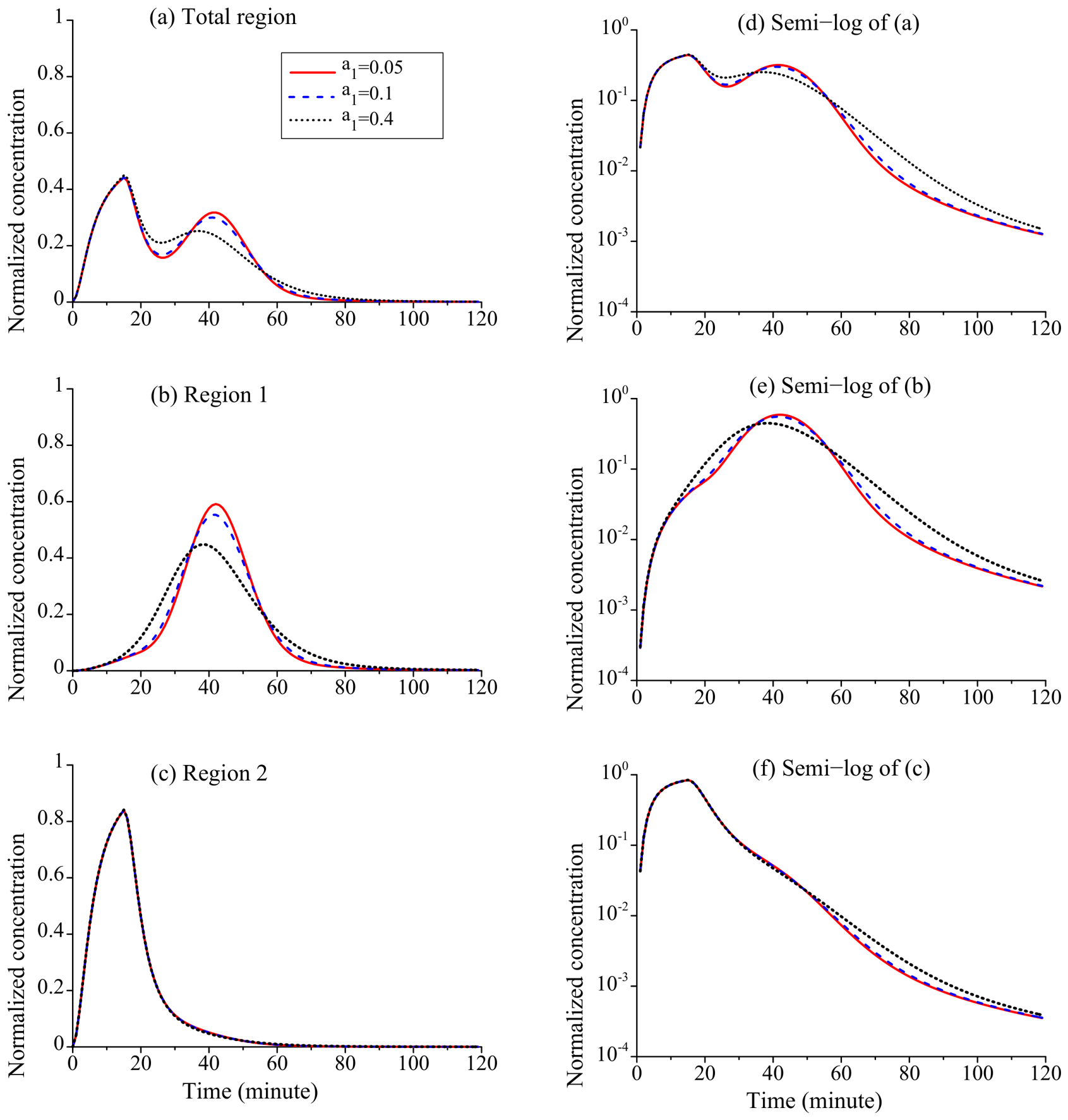
Figure 4 exhibits the concentration profiles in the total region, region 1, and region 2 under various dispersivities. The parameters are given as: θ 2 = 0.04 , a 2 = 4 ,   θ 1 = 0.1 , a 1 = 0.05 ,   0.1 ,   0.4 . The remaining parameters are listed in Table 1. As illustrated in Figure 4a, an increase in dispersivity in region 1 decreases the concentration value of the second peak. Similarly, it is observed that the peak concentration value in region 1 decreases with increasing dispersivity of region 1, and the concentration profiles in region 2 change slightly with varying dispersivities at the late-time tails. The mass exchange between region 1 and region 2 under various dispersivities is detailed in Section 4.3.

4.2. Effects of Sorption and Solute Retention on Anomalous Bimodal Transport in Layered Media

Solute transport in heterogeneous media usually exhibits non-Fickian transport behavior, which is attributed to solute retention or/and adsorption. The adsorption and retention of pollutants in the layered heterogeneous media (region 1 and region 2) are captured by the time-fractional derivative operators in our model, wherein the time index ( γ ) is the dominant parameter governing the sub-diffusion process. In this section, we focus on investigating the impact of media heterogeneity discrepancies on solute transport. The same inlet boundary condition used in Section 4.1 is applied here. For the sake of comparison, we assume fixed media parameters for region 2. The parameters are given as: γ 2 = 0.9 , β 2 = 0.2 , θ 2 = 0.04 , a 2 = 4 ,   γ 1 = 0.9 , 0.7 , 0.5 , β 1 = 0.2 , θ 1 = 0.1 , a 1 = 0.1 . The remaining parameters are presented in Table 1.
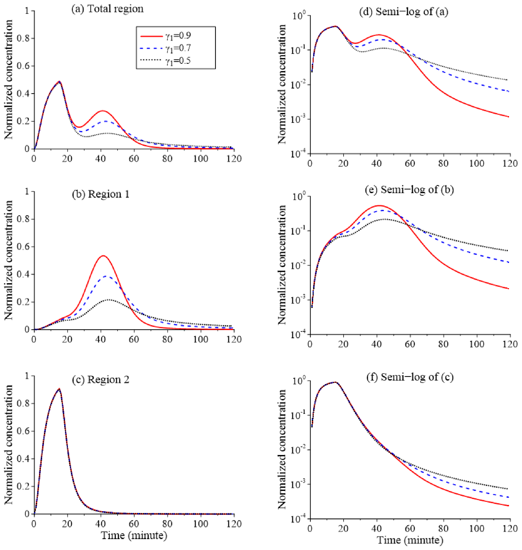
Figure 5 shows the velocity-averaged BTCs in the total region, region 1, and region 2 under various time indices γ 1 . The discrepancy of media heterogeneity between region 1 and region 2 has a significant effect on the non-Fickian transport. First, a smaller time index of region 1 ( γ 1 ) results in a lower concentration value of the second peak for the total region compared to cases with larger ( γ 1 ). This is because a decrease in time index ( γ 1 ) corresponds to the increase in solute retention or adsorption in region 1. Second, the power-law late-time tails become heavier with a decrease in the time index γ 1 for the total region, as more particles sample longer waiting times at late stages. Similarly, an increase in the time index enhances the peak concentration in region 1 and leads to weaker late-time tails. Changes to the time index affect the mass exchange between region 1 and region 2, which ultimately alters the late-time tails in the overall layered media. Detailed discussions follow in Section 4.3.

4.3. Mass Exchange Between Layered Regions

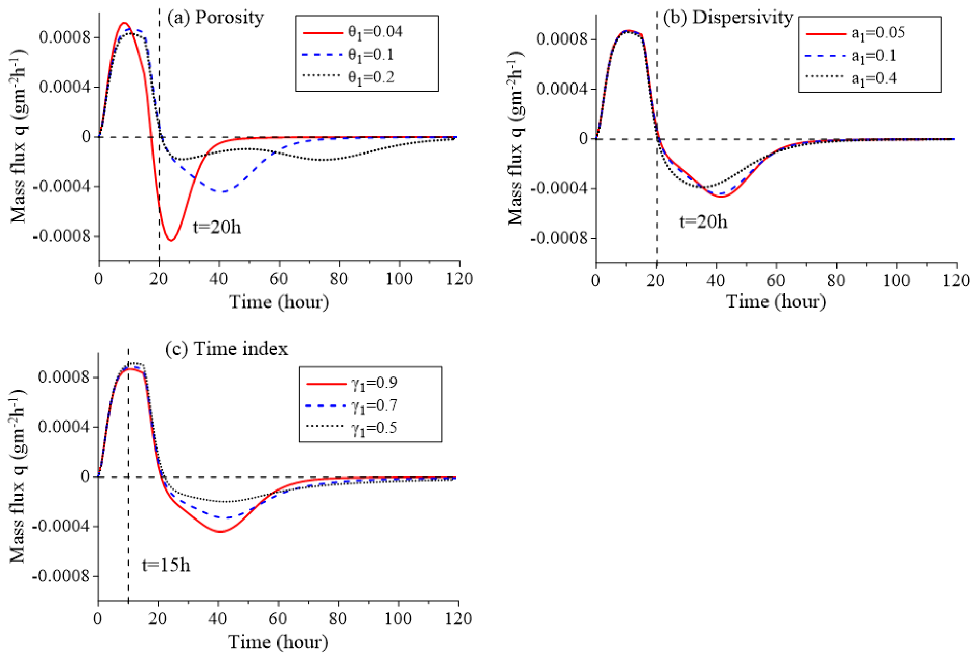
The mass exchange between the layered media (region 1 and region 2) directly reflects the effects of media properties on solute transport in the layered media. Figure 6 presents the time evolution of mass flux across the interface of region 1 and region 2 at the outlet. The parameters in Figure 6a, Figure 6b, and Figure 6c match those used in Figure 3, Figure 4, and Figure 5, respectively. A two-step mass transfer across the interface can be observed in Figure 6a. First, for cases with relatively larger porosity ( θ 1 = 0.1 , 0.2 ) of region 1, the mass flux increases with time, reaching a positive peak at t = 15 h during the injection period; afterward, it decreases to zero at t = 20 h during the flow flushing process. The positive mass flux during t < 15 h indicates solute transport from region 2 to region 1 via transverse dispersion; second, the mass flux continues to decrease until it reaches a peak negative value, after which it gradually increases and approaches zero. The negative mass flux during t 20 h implies the solute migration from region 1 back to region 2. We note that a substantially smaller porosity (red line for θ 1 = 0.04 ), which is close to the porosity of region 2, results in a shorter time for solute to reach peak mass flux. This is due to the higher velocity in region 1 resulting from the small porosity. In addition, the descending order of the late-time mass flux follows a similar trend to the late-time transport behavior of the solute under various porosities (Figure 3), since the late-time tails depend partially on the dispersion process from region 1 to region 2. Similar results can be observed in Figure 6b,c for various dispersivities and time indices. Moreover, a smaller time index in region 1 corresponds to a slower mass flux rate ( d q / d t ), leading to heavier late-time tails in the layered media.

4.4. Quantitative Parameter Sensitivity Analysis

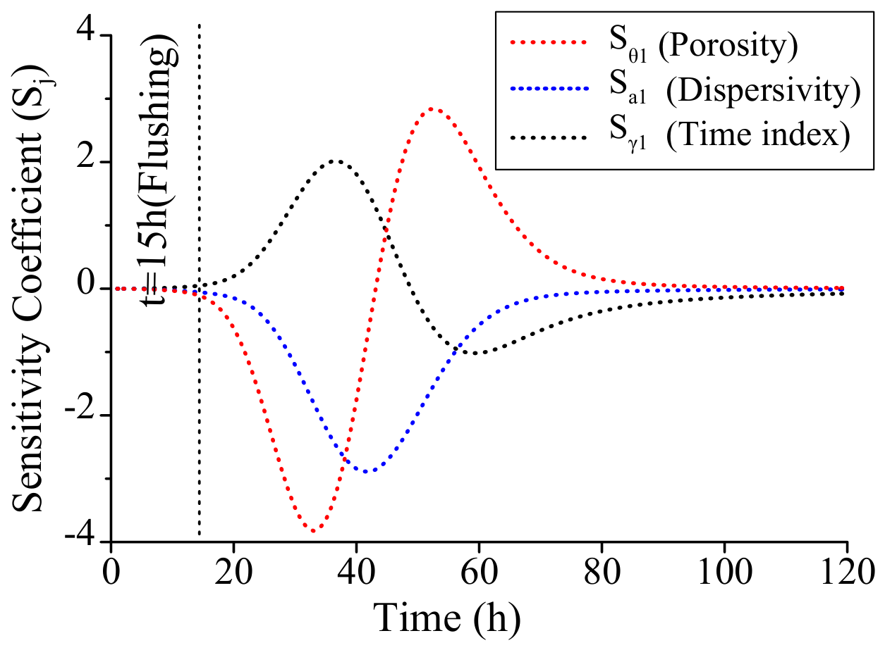
To quantitatively address the mechanisms governing the bimodal breakthrough curves (BTCs) and the late-time tailing, a local sensitivity analysis was conducted. The semi-normalized sensitivity coefficients S j for porosity θ 1 , dispersivity a 1 , and the fractional derivative index γ 1 were calculated and plotted against time (Figure 7).
During the injection phase ( t 15   h ), all sensitivity coefficients are approximately zero, quantitatively confirming that the first peak is entirely dominated by the fast advection in region 2, unaffected by region 1 properties. However, during the flushing process ( t > 15   h ), significant dynamic sensitivities emerge. The sensitivity coefficient of porosity ( S θ 1 ) exhibits the largest magnitude, characterized by a sharp negative trough at t 35   h followed by a positive peak at t 55   h . This phase-shift pattern provides rigorous mathematical evidence that θ 1 acts as the primary driving force governing the delayed release and the timing of the second concentration peak. Simultaneously, the dispersivity coefficient ( S a 1 ) remains strongly negative around the second peak ( t 40   h ), quantitatively verifying our previous observation that enhanced dispersivity attenuates the peak concentration.
Most notably, in the late-time tailing regime ( t > 60   h ), both S θ 1 and S a 1 rapidly decay to zero, indicating their diminished influence. In contrast, the sensitivity coefficient of the fractional index ( S γ 1 ) maintains a sustained negative value along the long tail. This negative sensitivity mathematically proves that a smaller time index γ 1 strictly dictates higher solute retention, thereby generating the heavier power-law tails observed in Section 4.2.

5. Applications

A field tracer experiment at the Savannah River Site (SRS) near Aiken, SC is utilized to investigate the applicability of the proposed model in capturing multi-peaked anomalous transport in layered aquifers [51]. The aquifer consists of sands and clayey sand with interbeds of clay, sandy clay, and gravel. The injection test site comprises six sampling wells and one injection well, where the sampling well is screened into four parts with intervals of 4.56 m. In each experiment, a constant injection flow rate (5.67 L min−1) was initially applied to the injection well for 24 h to establish a steady-state flow field. Then, a tritium-labeled solute was injected with a pulse duration ranging from 256 min to 560 min. Following the solute injection, non-labeled water was continuously pumped into the injection well for one week. The observed breakthrough curves of tritium in experiment B and experiment C for well S6, Zone 3, which exhibit apparent multi-peaked sub-diffusion, were selected for this study. For comparison, a traditional model based on the advection–dispersion equation (ADE) was also applied to fit the observed data. A detailed comparison of the time-fractional derivative models between the CTRW and MRMT frameworks is presented in Section S4 of the Supplementary Materials. In addition, detailed descriptions of the parameter sensitivity analysis, uncertainty analysis, statistical assessment of fitting quality, and discussions on parameter identifiability and uniqueness are provided in Section S3. The estimated parameters are listed in Table S2.
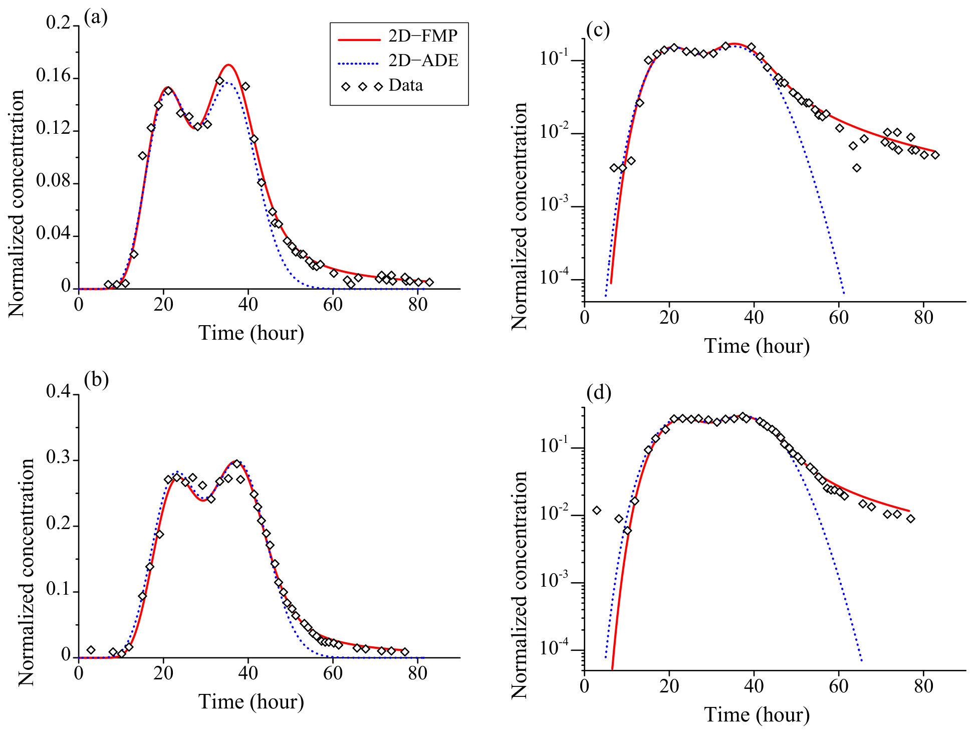
Figure 8 shows the simulated breakthrough curves for tritium using the 2D-FMP model and 2D-advection–dispersion equation (2D-ADE) model against the field tracer experiment data. The best-fit model parameters are listed in Table 2. The injection flow rate in the simulation was set constant and equal to that in the experiment. The results demonstrate that the 2D-FMP model successfully captures both the multi-peak behavior and the late-time tails observed in both experiments (experiment B and experiment C), which challenges the 2D-ADE model. This indicates that the 2D-FMP model is significantly more appropriate than the 2D-ADE model for capturing solute transport in heterogeneous layered porous media under non-uniform flow field, as it intrinsically accounts for the effects of the media property discrepancies, non-uniform velocity, and the local media heterogeneity.

6. Conclusions

This study investigated non-Fickian transport in heterogeneous layered porous media under a non-uniform flow velocity distribution. The transport of solute in such a system was successfully captured by a 2D-FMP model, in which the effects of media discrepancies are captured by two radial advection–dispersion equations coupled with vertical diffusion, while retention and adsorption effects are described by the fractional derivative operators. The relationship between media property discrepancies, media heterogeneity, and non-Fickian transport in layered media was systematically revealed. The model analysis and applications in this study lead to the following conclusions:
First, the discrepancies of media porosity and dispersivity within the layered porous media govern the anomalous bimodal transport behavior under a non-uniform velocity field. Two-peak transport behavior becomes more apparent as the discrepancy of media porosity increases. The peak value of the second peak decreases with an increase of θ 1 , while an increase in dispersivity in the slow region (region 1) decreases the concentration value of the second peak across the entire region.
Second, the discrepancies of media heterogeneity and tracer sorption between region 1 and region 2 also have a significant effect on both bimodal transport and sub-diffusion. A smaller time index of region 1 ( γ 1 ) results in relatively lower concentration value for the second peak in the total region, and the power-law late-time tails become heavier with a decrease in the time index γ 1 .
Third, the successful application of the 2D-FMP model reveals that solute transport in natural layered media usually exhibits complex anomalous bimodal transport behavior, a phenomenon arising from discrepancies in media properties and heterogeneity that the traditional 2D-ADE model fails to capture. The model analysis and application in this study significantly advance our understanding of the nature of anomalous bimodal transport in layered media, which provides powerful theoretical support for the remediation and long-term management of pollutants in natural systems.

Supplementary Materials

The following supporting information can be downloaded at: https://www.mdpi.com/article/10.3390/w18111309/s1, Figure S1: Mesh and time-step sensitivity analysis with different cases; Figure S2: Comparison between T-FADE, CTRW and MRMT; Table S1: Parameter Correlation Matrix (R) for 2D-FPM (Experiment B); Table S2: Parameter Correlation Matrix (R) for 2D-FPM (Experiment C).

Author Contributions

Conceptualization, D.Z., X.M., S.P. and X.C.; Formal analysis, D.Z.; Methodology, D.Z.; Software, D.Z.; Validation, D.Z.; Visualization, D.Z.; Writing—original draft, D.Z.; Data curation, D.Z.; Supervision, D.Z., X.M. and S.P.; Writing—review and editing, X.M., S.P. and X.C. All authors have read and agreed to the published version of the manuscript.

Funding

D.B. Zhou and S.L. Pan were supported by Scientific research startup fund of Anhui Polytechnic University (Grant No. 2022YQQ028), Anhui province housing and urban construction science and technology plan project (Grant No. 2024-YF030), Anhui Engineering University Excellent Youth Talent Fund Project (Grant No. 2021YQQ063), Scientific research projects of Anhui Polytechnic University (Grant No. Xjky2022167), Open Fund of the State Key Laboratory of Water Disaster Prevention (Grant No. 2024490911), Anhui Kaiste Automotive Technology Co., Ltd., Horizontal Entrustment (Grant No. HX-2025-12-055), and Nanjing Nanlan Environmental Protection Industry Co., Ltd., Horizontal Entrustment (Grant No. HX-2024-12-094).

Data Availability Statement

The original contributions presented in this study are included in the article. Further inquiries can be directed to the corresponding authors.

Conflicts of Interest

The authors declare that this study received funding from Anhui Kaiste Automotive Technology Co., Ltd. and Nanjing Nanlan Environmental Protection Industry Co., Ltd. The funder was not involved in the study design, collection, analysis, interpretation of data, the writing of this article, or the decision to submit it for publication.

References

  1. Zhou, L.; Selim, H.M. Solute transport in layered soils: Nonlinear and kinetic reactivity. Soil Sci. Soc. Am. J. 2001, 65, 1056–1064. [Google Scholar] [CrossRef]
  2. Sharma, P.K.; Sawant, V.A.; Shukla, S.K. Experimental and numerical simulation of contaminant transport through layered soil. Int. J. Geotech. Eng. 2014, 8, 345–351. [Google Scholar] [CrossRef]
  3. Bejat, L.; Perfect, E.; Quisenberry, V.L. Solute transport as related to soil structure in unsaturated intact soil blocks. Soil Sci. Soc. Am. J. 2000, 64, 818–826. [Google Scholar] [CrossRef]
  4. Tang, D.H.; Frind, E.O.; Sudicky, E.A. Contaminant transport in fractured porous media: Analytical solution for a single fracture. Water Resour. Res. 1981, 17, 555–564. [Google Scholar] [CrossRef]
  5. Chesnaux, R.; Rafini, S.; Elliott, A.P. A numerical investigation to illustrate the consequences of hydraulic connetions between granular and fractured-rock aquifers. Hydrogeol. J. 2012, 20, 1669–1680. [Google Scholar] [CrossRef]
  6. Tran, M.; Jha, B. Effect of poroelastic coupling and fracture dynamics on solute transport and geomechanical stability. Water Resour. Res. 2021, 57, e2021WR029584. [Google Scholar] [CrossRef]
  7. Karra, S.; O’Malley, D.; Hyman, J.D.; Viswanathan, H.S.; Srinivasan, G. Modeling flow and transport in fracture networks using graphs. Phy. Rev. E 2018, 97, 033304. [Google Scholar] [CrossRef]
  8. Rasmussen, T.C.; Haborak, K.G.; Young, M.H. Estimating aquifer hydraulic properties using sinusoidal pumping at the Savannah River site, South Carolina, USA. Hydrogeol. J. 2003, 11, 466–482. [Google Scholar] [CrossRef]
  9. Li, X.; Wen, Z.; Zhan, H. Laboratory observations for two-dimensional solute transport in an aquifer-aquitard system. Environ. Sci. Pollut. Res. 2021, 28, 38664–38678. [Google Scholar] [CrossRef]
  10. Barazzuoli, P.; Nocchi, M.; Rigati, R.; Salleolini, M. A conceptual and numerical model for groundwater management: A case study on a coastal aquifer in southern Tuscany, Italy. Hydrogeol. J. 2008, 16, 1557–1576. [Google Scholar] [CrossRef]
  11. Swami, D.; Sharma, P.K.; Ojha, C.S.P. Simulation of experimental breakthrough curves using multi-process non-equilibrium model for reactive solute transport in stratified porous media. Sadhana 2014, 39, 1425–1446. [Google Scholar] [CrossRef]
  12. Yin, M.; Ma, R.; Zhang, Y.; Wei, S.; Tick, G.R.; Wang, J.Q.; Sun, Z.Y.; Sun, H.G.; Zheng, C.M. A distributed-order time fractional derivative model for simulating bimodal sub-diffusion in heterogeneous media. J. Hydrol. 2020, 591, 125504. [Google Scholar] [CrossRef]
  13. Zhang, Y.; Zhou, D.B.; Yin, M.S.; Sun, H.G.; Wei, W.; Li, S.Y.; Zheng, C.M. Nonlocal transport models for capturing solute transport in one-dimensional sand columns: Model review, applicability, limitations, and improvement. Hydrol. Process. 2020, 34, 5104–5122. [Google Scholar] [CrossRef]
  14. Zhang, Y.; Meerschaert, M.M.; Baeumer, B.; LaBolle, E.M. Modeling mixed retention and early arrivals in multidimensional heterogeneous media using an explicit Lagrangian scheme. Water Resour. Res. 2015, 51, 6311–6337. [Google Scholar] [CrossRef]
  15. Rubin, Y. Flow and transport in bimodal heterogeneous formations. Water Resour. Res. 1995, 31, 2461–2468. [Google Scholar] [CrossRef]
  16. Dagan, G.; Lessoff, S.C. Solute transport in heterogeneous formations of bimodal conductivity distribution: 1. Theory. Water Resour. Res. 2001, 37, 465–472. [Google Scholar] [CrossRef]
  17. Coppola, A.; Comegna, V.; Basile, A.; Lamaddalena, N.; Severino, G. Darcian preferential water flow and solute transport through bimodal porous systems: Experiments and modelling. J. Contam. Hydrol. 2009, 104, 74–83. [Google Scholar] [CrossRef]
  18. Dunne, K.B.J.; Jerolmack, D.J. Evidence of, and a proposed explanation for, bimodal transport states in alluvial rivers. Earth Surf. Dyn. 2018, 6, 583–594. [Google Scholar] [CrossRef]
  19. Bijeljic, B.; Rubin, S.; Scher, H. Non-Fickian transport in porous media with bimodal structural heterogeneity. J. Contam. Hydrol. 2011, 120, 213–221. [Google Scholar] [CrossRef] [PubMed]
  20. Dentz, M.; Tartakovsky, D.M. Delay mechanisms of non-Fickian transport in heterogeneous media. Geophys. Res. Lett. 2006, 33, L16406. [Google Scholar] [CrossRef]
  21. Coats, K.H.; Smith, B.D. Dead-end pore volume and dispersion in porous media. Soc. Pet. Eng. J. 1964, 4, 73–84. [Google Scholar] [CrossRef]
  22. Skopp, J.; Gardner, W.R.; Tyler, E.J. Solute movement in structured soils: Two-region model with small interaction. Soil Sci. Soc. Am. J. 1981, 45, 837–842. [Google Scholar] [CrossRef]
  23. Field, M.S.; Leij, F.J. Solute transport in solution conduits exhibiting multi-peaked breakthrough curves. J. Hydrol. 2012, 440, 26–35. [Google Scholar] [CrossRef]
  24. Wang, C.; Wang, X.; Majdalani, S.; Guinot, V.; Jourde, H. Influence of dual conduit structure on solute transport in karst tracer tests: An experimental laboratory study. J. Hydrol. 2020, 590, 125255. [Google Scholar] [CrossRef]
  25. Markale, I.; Velásquez-Parra, A.; Alcolea, A. Mixing controlled adsorption at the liquid-solid interfaces in unsaturated porous media. Transp. Porous Media 2023, 146, 159–175. [Google Scholar] [CrossRef] [PubMed]
  26. Haggerty, R.; Gorelick, S.M. Multiple-rate mass transfer for modeling diffusion and surface reactions in media with pore-scale heterogeneity. Water Resour. Res. 1995, 31, 2383–2400. [Google Scholar]
  27. Tecklenburg, J.; Neuweiler, I.; Carrera, J. Multi-rate mass transfer modeling of two-phase flow in highly heterogeneous fractured and porous media. Adv. Water Resour. 2016, 91, 63–77. [Google Scholar] [CrossRef]
  28. Berkowitz, B.; Cortis, A.; Dentz, M.; Harvey, S. Modeling non-Fickian transport in geological formations as a continuous time random walk. Rev. Geophys. 2006, 44, RG2003. [Google Scholar] [CrossRef]
  29. Burnell, D.K.; Hansen, S.K.; Xu, J. Transient modeling of non-Fickian transport and first-order reaction using continuous time random walk. Adv. Water Resour. 2017, 107, 370–392. [Google Scholar] [CrossRef]
  30. Hansen, S.K. Experimental support for a simplified approach to CTRW transport models and exploration of parameter interpretation. Water Resour. Res. 2022, 58, e2021WR031350. [Google Scholar] [CrossRef]
  31. Schumer, R.; Benson, D.A.; Meerschaert, M.M.; Baeumer, B. Fractal mobile/immobile solute transport. Water Resour. Res. 2003, 39, 1296. [Google Scholar] [CrossRef]
  32. Meerschaert, M.M.; Zhang, Y.; Baeumer, B. Tempered anomalous diffusion in heterogeneous systems. Geophys. Res. Lett. 2008, 35, L17403. [Google Scholar] [CrossRef]
  33. Zhou, D.B.; Brusseau, M.L.; Zhang, Y.; Li, S.; Wei, W.; Sun, H.; Zheng, C. Simulating PFAS adsorption kinetics, adsorption isotherms, and nonideal transport in saturated soil with tempered one-sided stable density (TOSD) based models. J. Hazard. Mater. 2021, 411, 125169. [Google Scholar] [CrossRef]
  34. Alam, M.P.; Khan, A.; Baleanu, D. A high-order unconditionally stable numerical method for a class of multi-term time-fractional diffusion equation arising in the solute transport models. Int. J. Comput. Math. 2023, 100, 105–132. [Google Scholar] [CrossRef]
  35. Dentz, M.; Berkowitz, B. Transport behavior of a passive solute in continuous time random walks and multirate mass transfer. Water Resour. Res. 2003, 39, 1111. [Google Scholar] [CrossRef]
  36. Houssais, M.; Lajeunesse, E. Bedload transport of a bimodal sediment bed. J. Geophys. Res. 2012, 117, F04015. [Google Scholar] [CrossRef]
  37. Zhang, Y.; Green, C.T.; Baeumer, B. Linking aquifer spatial properties and non-Fickian transport in mobile–immobile like alluvial settings. J. Hydrol. 2014, 512, 315–331. [Google Scholar] [CrossRef]
  38. Yang, Z.W.; Zheng, X.C.; Wang, H. A variably distributed-order time-fractional diffusion equation: Analysis and approximation. Comput. Methods Appl. Mech. Eng. 2020, 367, 113118. [Google Scholar] [CrossRef]
  39. Chen, J.S.; Chen, C.S.; Chen, C.S. Analysis of solute transport in a divergent flow tracer test with scale-dependent dispersion. Hydrol. Process. 2007, 21, 2526–2536. [Google Scholar] [CrossRef]
  40. Suk, H.; Chen, J.S.; Han, W.S. New semi-analytical solutions to the radial advection-dispersion equation for solute transport in a transient divergent radial flow. Adv. Water Resour. 2022, 167, 104283. [Google Scholar] [CrossRef]
  41. Huang, C.S.; Tong, C.; Hu, W.S.; Yeh, H.D.; Yang, T. Analysis of radially convergent tracer test in a two-zone confined aquifer with vertical dispersion effect: Asymmetrical and symmetrical transports. J. Hazard. Mater. 2019, 377, 8–16. [Google Scholar] [CrossRef]
  42. Suk, H.; Han, W.S.; Chen, J.S. Semi-analytical solution of single-well push–pull test under transient flow conditions. J. Hydrol. 2023, 620, 129542. [Google Scholar] [CrossRef]
  43. Li, X.; Wen, Z.; Zhu, Q.; Jakada, H. A mobile-immobile model for reactive solute transport in a radial two-zone confined aquifer. J. Hydrol. 2020, 580, 124347. [Google Scholar] [CrossRef]
  44. Landkamer, L.L.; Harvey, R.W.; Scheibe, T.D. Colloid transport in saturated porous media: Elimination of attachment efficiency in a new colloid transport model. Water Resour. Res. 2013, 49, 2952–2965. [Google Scholar] [CrossRef]
  45. Bradford, S.A.; Simunek, J.; Bettahar, M.; van Genuchten, M.T.; Yates, S.R. Modeling colloid attachment, straining, and exclusion in saturated porous media. Environ. Sci. Technol. 2003, 37, 2242–2250. [Google Scholar] [CrossRef]
  46. Lv, X.; Sun, Y.; Ji, R. Physicochemical factors controlling the retention and transport of perfluorooctanoic acid (PFOA) in saturated sand and limestone porous media. Water Res. 2018, 141, 251–258. [Google Scholar] [CrossRef]
  47. Bi, Y.; Jiang, Z. The finite volume element method for the two-dimensional space-fractional convection–diffusion equation. Adv. Differ. Equ. 2021, 2021, 379. [Google Scholar] [CrossRef]
  48. Para, K.; Sungnul, S.; Sirisubtawee, S. A Comparison of Numerical Solutions for Advection-Diffusion-Reaction Equations between Finite Volume and Finite Difference Methods. Eng. Lett. 2022, 30, 1–16. [Google Scholar]
  49. Lai, W.; Ogden, F.L. A mass-conservative finite volume predictor–corrector solution of the 1D Richards’ equation. J. Hydrol. 2015, 523, 119–127. [Google Scholar] [CrossRef]
  50. Liang, X.; Zhang, Y.K.; Liu, J. Solute transport with linear reactions in porous media with layered structure: A semianalytical model. Water Resour. Res. 2019, 55, 5102–5118. [Google Scholar] [CrossRef]
  51. Seaman, J.C.; Bertsch, P.M.; Wilson, M. Tracer migration in a radially divergent flow field: Longitudinal dispersivity and anionic tracer retardation. Vadose Zone J. 2007, 6, 373–386. [Google Scholar] [CrossRef]
Figure 1. Schematic diagram of solute transport in a structured porous medium.
Water 18 01309 g001
Figure 2. Computed BTCs using the 2D-FMP model (13–14) (red lines) and radial transport model (Equation (4) in Chen et al. (2007) [39]) (symbols) for the control plane located at x = 2 m (a), x = 4 m (b), and x = 6 m (c). The transverse dispersion and fractional capacity in the 2D-FMP model (13–14) are set to zero.
Water 18 01309 g002
Figure 3. Velocity-averaged concentration profiles along the z-direction for the total domain (a) region 1 (b) and region 2 (c) under various porosities of region 1 with θ 1 = 0.04, 0.1, and 0.2, respectively. The right Figures (df) are the semi-log plots of the left ones, to show the late-time tail of the BTC.
Water 18 01309 g003
Figure 4. Velocity-averaged concentration profiles along the z-direction for the total domain (a) region 1 (b) and region 2 (c) under various dispersivities (a) of region 1 with a 1 = 0.05, 0.1, and 0.4, respectively. The right Figures (df) are the semi-log plots of the left ones, to show the late-time tail of the BTC.
Water 18 01309 g004
Figure 5. Velocity-averaged concentration profiles along the z-direction for the total domain (a) region 1 (b) and region 2 (c) under various time indices of region 1 with γ 1 = 0.9, 0.7, and 0.5, respectively. The right Figures (df) are the semi-log plots of the left ones, to show the late-time tail of the BTC.
Water 18 01309 g005
Figure 6. Comparison of mass exchange across the interface of region 1 and region 2 under various porosities, dispersivities, and time indices.
Water 18 01309 g006
Figure 7. Temporal distributions of the normalized sensitivity coefficient S j to parameters porosity θ 1 ( S θ 1 ), dispersivity a 1 ( S a 1 ), and the fractional derivative index γ 1 ( S γ 1 ).
Water 18 01309 g007
Figure 8. Measured (symbols) versus simulated (lines) breakthrough curves for tritium transport in aquifer in experiment B (a) and experiment C (b). The lines are the best-fit solutions using the 2D-FMP model (13–14) and the 2D-ADE model, respectively. (c,d) are the semi-log plots of (a,b), respectively, to show the late-time tail.
Water 18 01309 g008
Table 1. Parameters for the base case used in this paper.
ParameterSymbolValue
Region length L12 m
Injection rateQ4 m3/h
Width of region 2B2.5 m
Porosity of region 2 θ 2 0.04
Dispersivity of region 2 a 2 4 m
Capacity of region 2 β 2 0.2
Time index of region 2 γ 2 0.9
Transverse diffusion D z 1 , D z 2 0.0024 m2/h
Table 2. Summary of the 2D-FMP model parameters with 95% confidence intervals (CIs) applied to the field tracer experiment data.
Experiment a 1 (m) γ 1 (−) β 1 ( h α 1 1 ) θ 1 (−) D z 1 (m2/h) a 2 (m) γ 2 (−) β 2 ( h α 2 1 ) θ 2 (−) D z 2 (m2/h)RMSENSE
B0.009 ±   0.001 0.7 ±   0.024 0.13
±   0.014
0.550.00240.08 ±   0.002 0.44
±   0.018
0.062
±   0.022
0.180.00240.02140.950
C0.012 ±   0.005 0.72 ±   0.023 0.11
±   0.022
0.550.00240.05 ±   0.003 0.44
±   0.017
0.070
±   0.015
0.180.00240.02350.921
Disclaimer/Publisher’s Note: The statements, opinions and data contained in all publications are solely those of the individual author(s) and contributor(s) and not of MDPI and/or the editor(s). MDPI and/or the editor(s) disclaim responsibility for any injury to people or property resulting from any ideas, methods, instructions or products referred to in the content.