Spatio-Temporal Evaluation and Attribution Analysis of Urban Flood Resilience in the Beijing–Tianjin–Hebei Region: A Multi-Method Coupling Approach

Abstract

Urban floods increasingly threaten the mega-regions’ sustainable development, yet the pace and causes of change in urban flood resilience (UFR) remain elusive. This study proposes a new index system for UFR from three dimensions: resistance, recovery, and adaptability. The system includes 18 indicators across natural, economic, social, and infrastructure aspects. A comprehensive evaluation model combining entropy weighting, Criteria Importance Through Intercriteria Correlation (CRITIC), and VlseKriterijumska Optimizacija I Kompromisno Resenje (VIKOR) methods is developed and validated for the Beijing–Tianjin–Hebei (BTH) region of China, covering 2011–2022. Spatial dependence is diagnosed with global and local Moran’s I statistics, while an Extreme Gradient Boosting-Shapley Additive Explanations (XGBoost-SHAP) isolates the contribution of each driver. The results indicate that UFR in the BTH region exhibited a generally increasing but fluctuating trend. Spatially, UFR displays a pronounced gradient, with higher levels concentrated in the northwest and lower levels in the southeast. Significant spatial autocorrelation is observed, spatial autocorrelation strength ranging from 0.330 to 0.404. Key drivers contributing to UFR include urban slope, hydrological station density, per capita park green space area, and population density, all with SHAP importance values exceeding 0.02 (ranging from 0.0012 to 0.1343). These indicators collectively play a dominant role in shaping the region’s resilience dynamics, highlighting their crucial influence on sustainable urban development.

1. Introduction

Global urbanization, a key feature of contemporary socio-economic transformation, has led to increased concentration of production factors and population in urban areas. While this stimulates regional economic growth, it also heightens the vulnerability of urban systems to environmental and infrastructural stresses. China’s urbanization rate grew from 17.92% in 1978 to 65.22% in 2022, accompanied by an annual increase of 12.6% in urban natural disaster losses over the past decade, with floods accounting for 73.6% of the losses [1]. The Beijing–Tianjin–Hebei (BTH) region, though covering only 1.9% of China’s land, houses 7.8% of the population and contributed 9.3% to the national Gross Domestic Product (GDP) in 2022. However, a 2023 flood in the Haihe River Basin caused losses exceeding 100 billion yuan (CNY), revealing the gap between traditional flood control infrastructure and urban development needs [2]. Conventional flood control methods are increasingly inadequate, while the emerging paradigm of resilient cities—focusing on self-organization and adaptability—offers a promising solution for overcoming existing flood management challenges and enhancing urban resilience amid climate and hydrological uncertainties [3,4,5,6,7]. Resilience, originally an engineering concept for structural recovery, has evolved into a broader framework. It now focuses on dynamic self-organization and system transitions in complex adaptive systems, significantly influencing urban resilience studies [8,9,10,11].

Scholars have made notable progress in advancing the study of UFR, contributing to a growing body of theoretical frameworks, influencing indicators, and empirical applications. In terms of evaluation frameworks, Oladokun et al. [12] employed fuzzy logic methods to conduct an abstract analysis of flood resilience systems. By identifying system variables and parameters, they established a flood resilience framework from three perspectives: natural, socio-technical, and socio-economic, and validated the model using raw data from flood-prone communities in southwestern Nigeria. Karamouz et al. [13] developed a dynamic urban infrastructure resilience assessment equation based on four dimensions: agility, robustness, redundancy, and resource accessibility, aimed at improving infrastructure resilience in New York City. Simonovic et al. [14] developed the Flood Resilience Simulation Tool (FRST) to help quantify, compare, and visualize dynamic flood resilience. Chen et al. [15] established a resilience assessment model for rainstorm and flood scenarios, focusing on three attributes: resistance, recovery, and adaptability, which comprehensively consider the various capacities of cities when facing rainstorm and flood disasters. Xiao et al. [16] constructed an UFR assessment system from the PSR (Pressure-State-Response) perspective, analyzing the pressure, state, and response processes of urban flood systems from three angles: stimulus, sensitivity, and adaptability. Li et al. [17] quantified UFR based on the “4R” characteristics—robustness, resource, responsiveness, and redundancy. He et al. [18] developed a flood resilience evaluation index system based on the dimensions of economy, society, environment, and infrastructure construction. Bao et al. [19] developed a comprehensive “Risk-Resilience-Effect” framework, based on the MaxEnt model and the interpretable XGBoost-SHAP model. The study primarily revealed the trade-offs and synergies between flood risk and resilience, and quantified the nonlinear threshold effects of key influencing factors.

In the exploration of influencing indicators, existing studies mainly apply methods such as gray relational analysis, obstacle degree models, spatial Durbin models, and geographical spatial detectors, among others. Ji et al. [20] used gray relational analysis to diagnose the importance of indicators influencing urban resilience from a rainstorm and flood perspective. Song et al. [21], based on the obstacle degree model, analyzed the key limiting indicators hindering the development of flood resilience in cities at different types and stages of development. Zhang et al. [22] employed the spatial Durbin model, considering both spatial spillover effects and spatial heterogeneity, to deeply analyze the influencing indicators in the Yellow River basin and its upper, middle, and lower reaches. Chen et al. [23] applied the geographical detector model, which can explain the spatial differentiation of UFR and analyze its internal driving mechanisms.

Through the above review, two areas for improvement in current UFR research can be identified: Firstly, most scholars’ interpretations and understandings of UFR are limited to process mechanisms or isolated urban indicators. However, UFR is a complex, multi-dimensional concept. By approaching it from the dimensions of resistance, recovery, and adaptability, and coupling multi-source indicators from nature, economy, society, and infrastructure, a more systematic and comprehensive evaluation framework can be developed. Secondly, in exploring the influencing indicators, commonly used methods such as the obstacle degree model are effective in identifying key indicators but struggle to quantitatively explain the specific contributions of each indicator to changes in UFR. These methods also have limited capabilities in handling nonlinear relationships and complex interaction effects. The XGBoost-SHAP method combines machine learning’s efficient processing power with strong interpretability. It improves prediction accuracy for complex UFR driving indicators and reveals the quantitative contributions and directional impacts of each indicator. This method offers better interpretability and higher practical value [19,24,25].

Given the complexity of urban systems and flood processes, urban flood resilience evaluation involves multiple levels, objectives, and attributes, often accompanied by conflicts among indicators. Therefore, multi-attribute decision-making (MCDM) methods are particularly suitable for this type of assessment. Among various MCDM approaches, the VIKOR method was adopted because it is specifically designed to address conflicting criteria and to identify a compromise solution by measuring proximity to the ideal solution, which is consistent with the trade-offs among resistance, recovery, and adaptability dimensions in UFR assessment. In terms of indicator weighting, the CRITIC method was selected instead of subjective approaches such as AHP, as it objectively determines weights by considering both the contrast intensity and the conflict among indicators. This avoids expert bias and better reflects the inherent information structure of the data. By incorporating information entropy to characterize indicator dispersion, the CRITIC-based weighting ensures scientifically reliable and robust weight assignment.

Therefore, this study constructs an indicators system of UFR from the process perspective of resistance, recovery, and adaptability, which considers the perspectives of nature, economy, society, and infrastructure. Index weights are determined using the CRITIC method, which integrates entropy weighting. UFR levels of 13 cities in the BTH region from 2011 to 2022 are evaluated using the VIKOR method [26]. Additionally, the widely applicable XGBoost-SHAP model is employed to identify driving indicators, supporting the development of strategies to improve UFR in the BTH region.

This study focuses on the BTH region, providing an in-depth analysis of the concept of flood resilience. It incorporates spatiotemporal evolution analysis to specifically explore how UFR changes over time and responds to social and environmental dynamics. Furthermore, by integrating the XGBoost-SHAP model with MCDM methods, this study offers a more comprehensive framework for assessing UFR [19].

2. Materials and Methods

2.1. Study Area

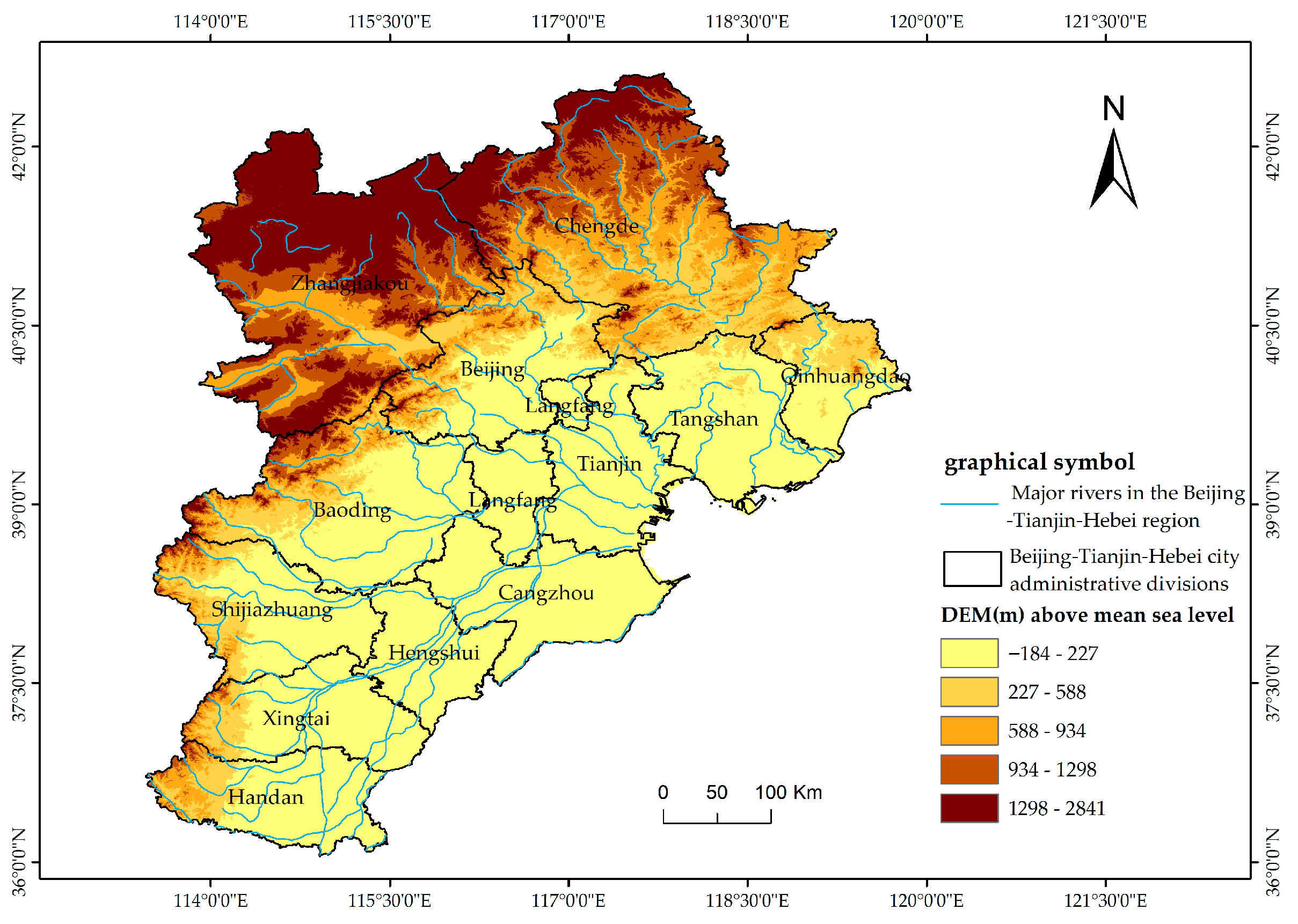
The BTH region consists of Beijing, Tianjin, and 11 cities in Hebei Province, namely Chengde, Zhangjiakou, Qinhuangdao, Tangshan, Baoding, Langfang, Cangzhou, Shijiazhuang, Handan, Xingtai, and Hengshui, as shown in Figure 1.

The BTH region covers an area of 215,300 km² and has a typical warm-temperate, semi-humid to semi-arid continental monsoon climate. The average annual temperature ranges from 8 to 12 °C, and the average annual precipitation is approximately 500 mm. However, there is significant spatial and temporal heterogeneity: 60–80% of the precipitation occurs during the flood season from June to August. The windward slope of the Yanshan Mountains forms a rainy zone, with annual precipitation ranging from 700 to 800 mm, while the northern plateau receives less than 400 mm [27]. The region is drained by two major river systems: the Hai River and the Luan River. The Hai River system consists of the main stream and five major tributaries—North Canal, Yongding River, Daqing River, Ziya River, and South Canal. The Luan River system includes the Luan River and its neighboring rivers, which flow through cities such as Chengde and Tangshan. Additionally, lakes and wetlands are widely distributed in the region, including Baiyangdian and Hengshui Lake.

2.2. Evaluation Index System Construction

UFR refers to the comprehensive ability of urban systems to maintain essential functions and absorb impacts in the face of flooding disturbances. It also involves the capacity for dynamic adjustments and transformative development through the integration of subsystems such as natural, economic, social, and infrastructure systems.

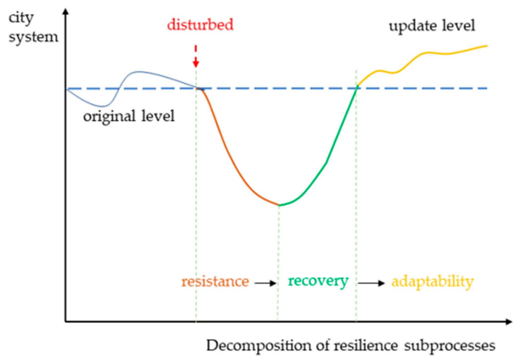
The evolution of resilience can be viewed as a cyclical process. In Figure 2, the city system represents the urban system’s structure and function under external disturbances. Disturbed refers to the impact of flood disasters, causing deviation from the original state. The original level is the normal operating state of the city without external disturbances, reflecting stability. The update level indicates the development achieved after resistance, recovery, and adaptability [28].

Urban systems undergo three stages after being disturbed: resistance, recovery, and adaptability. These stages are demarcated based on the system’s temporal and functional responses to flood disturbances. Resistance is the foundational dimension of UFR, representing the ability of urban systems to withstand floods. It is characterized by the system’s ability to maintain structural stability and functional continuity, relying on infrastructure and flood control measures. This phase occurs immediately after the disturbance and is marked by a sharp deviation from the original level. Recovery refers to the urban system’s ability to return to a stable state after a disturbance. It emphasizes the restoration of socio-economic activities and the normalization of residents’ lives. This phase begins after the immediate impacts subside and focuses on regaining normal operational capacity, marked by a gradual return to the original level. Adaptability is the advanced dimension of UFR, referring to the urban system’s ability to reach a higher level through learning and adjustment to future risks. It involves urban planning, policy changes, and social and economic transformations to enhance long-term resilience. This phase is demarcated by the system’s ability to evolve beyond its original capacity, achieving an “update level.” These stages reflect the system’s capacity to absorb immediate impacts, restore functions, and adapt for future resilience. The decline represents resistance, the rise corresponds to recovery, and the upward trajectory signifies adaptability.

Based on existing research on urban resilience assessment and the analysis of resilience mechanisms [15], and considering the four components of urban systems—natural, economic, social, and infrastructure—eighteen flood resilience indicators were ultimately selected [29], as shown in

Table 1. Indicator system.

Criterion Layer	Indicator Layer	Attribute	Category	Reference
Resistance	Urban population density (A1)	−	Society	[30,31]
	Greening coverage ratio in built-up areas (A2)	+	Nature	[31,32]
	Annual precipitation (A3)	−	Nature	[30,33]
	Average urban slope (A4)	+	Nature	[31,32]
	Drainage pipeline density (A5)	+	Infrastructure	[30,33]
Recovery	Registered urban unemployment rate (B1)	−	Society	[31,33]
	Health technicians per 10,000 population (B2)	+	Society	[31,34]
	Health insurance coverage rate (B3)	+	Society	[30,31]
	Proportion of vulnerable groups in the community (B4)	−	Society	[30,31]
	Per capita disposable income of urban residents (B5)	+	Economy	[31,34]
	Share of tertiary-sector value added in GDP (B6)	+	Economy	[31,33]
	Per capita urban road area (B7)	+	Infrastructure	[33,34]
	Wastewater treatment rate (B8)	+	Infrastructure	[30,31]
Adaptability	Flood prevention and disaster mitigation policies (C1)	+	Society	[30,35]
	Per capita park green space area (C2)	+	Nature	[31,33]
	R&D expenditure as a share of GDP (C3)	+	Economy	[30,31]
	Per capita general public budget expenditure (C4)	+	Economy	[33,34]
	Hydrological station density (C5)	+	Infrastructure	[31,32]

. All indicators are classified as positive (+), where a larger value is better, or negative (−), where a smaller value is better.

Resistance represents the ability of urban systems to withstand the impacts of flooding. Urban population density reflects the city’s basic carrying capacity and indicates the efficiency of spatial resource allocation. Higher density can lead to greater strain on infrastructure and resources during a flood, affecting resistance. Annual precipitation volume directly determines the intensity of flooding, it provides a stable measure of long-term climate and rainfall patterns, reflecting the changing flood risk over time. Larger volumes of rainfall lead to more severe flooding, thereby reducing resistance to flood impacts. A higher green coverage rate improves the infiltration of rainwater and reduces surface runoff, enhancing the city’s resistance to flooding by allowing better water absorption. Steeper slopes allow for faster runoff, preventing the accumulation of large amounts of water in low-lying areas, thereby enhancing flood resistance. A higher density of drainage pipes improves the flood discharge effectiveness per unit area, directly increasing the city’s resistance to flooding by enhancing water flow management.

Recovery represents the ability of urban systems to return to a stable state. The urban registered unemployment rate reflects the level of human resources in the city. A lower unemployment rate indicates a stronger labor force, which directly accelerates post-disaster economic recovery by supporting the reconstruction of industries and services. The number of healthcare professionals indicates the capacity for medical support. A higher number of healthcare professionals ensures a timely and effective response to health emergencies, which is crucial for recovery after a disaster. The coverage of medical insurance reflects the inclusivity of the city’s social security system. A higher coverage rate reduces the financial burden on individuals after a disaster, contributing to a smoother recovery process. The proportion of vulnerable groups reflects the vulnerability of the urban community population structure. A higher proportion of vulnerable groups (such as the elderly and children) may slow recovery, as these groups require additional resources for rehabilitation. A balanced dependency ratio can help mitigate this impact by providing adequate labor support for recovery. The per capita disposable income of urban residents indicates individual economic levels. Higher disposable income allows individuals and families to recover faster by rebuilding their homes and businesses, thus contributing to the overall recovery process. The proportion of value added by the tertiary sector is an indicator of industrial upgrading. An economy dominated by the service sector is more flexible and can recover more quickly from disasters, as it is less dependent on physical infrastructure than industries in the primary and secondary sectors. Per capita urban road area serves as a basic indicator of road network capacity. Adequate road infrastructure is essential for ensuring accessibility during recovery, as it facilitates the movement of goods, services, and people for disaster relief. The sewage treatment rate indicates the municipal department’s ability to manage daily sewage and control the spread of pollution. An effective sewage treatment system is critical for maintaining public health and preventing disease outbreaks during recovery.

Adaptability represents the ability of urban systems to achieve sustainable development through learning and adjustment. Flood control and disaster reduction policies serve as institutional safeguards for the city’s response to flood risks, determining the systematization and foresight of urban flood management efforts. These policies not only shape flood risk management strategies but also influence the overall adaptive capacity of urban systems. Per capita park green space can effectively enhance surface water retention capacity. Larger areas of park green space improve the absorption of rainwater, mitigating the impact of heavy rainfall. The proportion of R&D expenditure to GDP is a key indicator of the city’s investment intensity in technological innovation. A higher proportion of R&D expenditure signifies a greater capacity for developing disaster response technologies. Per capita general public budget expenditure provides the material foundation for implementing emergency preparedness. Adequate public funding ensures that cities can implement effective flood risk management strategies, and improve the overall adaptive capacity of urban systems. The density of hydrological stations provides data support for early warning of flood disasters, enabling cities to adjust flood control strategies proactively. A higher density of stations ensures timely and accurate flood predictions, which help prevent passive responses due to delayed information and enhance the city’s adaptive capacity.

2.3. Data Sources

The data used in this study were sourced from the following channels: the China Urban Statistical Yearbook: annual data on urban population, infrastructure, and socio-economic factors were provided (A1, A2, A5, B4, B7, C2, C5, accessed on 5 March 2025). The China Meteorological Disasters Yearbook: data on meteorological events were provided (A3, accessed on 5 March 2025). The National Economic and Social Development Statistical Bulletin of each city: economic and social data for each city were provided, compiled annually (B1, B2, B3, B8, C1, C3, accessed on 11 March 2025). The National Bureau of Statistics, the Hebei Economic Yearbook (2012–2019) and the Hebei Statistical Yearbook (2020–2023): economic performance data for all cities were contained, published annually (B5, B6, C4, accessed on 11 March 2025). The Geospatial Data Platform: the Geospatial Data Cloud was used (A4, accessed on 11 March 2025). Missing data points were interpolated using linear interpolation based on adjacent years, as the missing values were isolated (i.e., data from non-contiguous years were missing).

2.4. CRITIC-Entropy Weight Combination Assignment Method

The CRITIC method is an objective weighting technique that allocates weights by analyzing the intensity and conflict between indicators. It uses the coefficient of variation to quantify the degree of variation in indicator data, while the Pearson correlation matrix captures the interdependencies between them. However, the traditional CRITIC model has two main limitations: first, it does not distinguish between the effects of positive and negative correlations on weight allocation; and second, it fails to consider the nonlinear dispersion of indicators, making it challenging to fully capture interactions between indicators in complex systems using only linear correlation.

To address these limitations, we integrate the Entropy Weight Method, which calculates weights based on the degree of data dispersion, using information entropy theory. Higher dispersion leads to lower entropy values, resulting in higher weights for more variable indicators.

Given the multi-source nature of data in UFR research, a single weighting method cannot fully account for both indicator interrelations and data dispersion. Therefore, we combine the CRITIC method with the Entropy Weight Method, creating a more comprehensive and effective weighting model.

2.4.1. CRITIC Weighting

CRITIC determines the information content of indicators based on their comparative strength and conflict.

Step 1: Data standardization [36].

For positive indicator ${\mathrm{x}}_{ij}$:

$$y_{ij}=0.001+0.998{\displaystyle \frac{{\mathrm{x}}_{ij}-\underset{i}{\min }\{{\mathrm{x}}_{ij}\}}{\underset{i}{\max }\{{\mathrm{x}}_{ij}\}-\underset{i}{\min }\{{\mathrm{x}}_{ij}\}}}$$

(1)

For negative indicator ${\mathrm{x}}_{ij}$:

$$y_{ij}=0.001+0.998{\displaystyle \frac{\underset{i}{\max }\{{\mathrm{x}}_{ij}\}-{\mathrm{x}}_{ij}}{\underset{i}{\max }\{{\mathrm{x}}_{ij}\}-\underset{i}{\min }\{{\mathrm{x}}_{ij}\}}}$$

(2)

Step 2: Calculation of the standard deviation for each indicator. For each standardized evaluation indicator, the standard deviation is calculated to represent the degree of fluctuation of the indicator. A larger standard deviation indicates greater variability in the indicator across the samples, implying richer information. The formula for calculating the standard deviation is:

$${\mathrm{\sigma }}_j=\sqrt{{\displaystyle \frac{1}{n-1}}{\displaystyle \sum _{i=1}^n{(x_{ij}-\stackrel{-}{x_j})}^2}}$$

(3)

where $x_{ij}$ represents the standardized data and $\stackrel{-}{x_j}$ denotes the mean of the jth indicator.

Step 3: Calculation of correlation between indicators. For each pair of indicators j and k, their correlation is calculated as follow:

$${\rho }_{jk}={\displaystyle \frac{{\displaystyle \sum _{i=1}^n(x_{ij}-\stackrel{-}{x_j})(x_{ik}-\stackrel{-}{x_k})}}{\sqrt{{\displaystyle \sum _{i=1}^n{(x_{ij}-\stackrel{-}{x_j})}^2{\displaystyle \sum _{i=1}^n{(x_{ik}-\stackrel{-}{x_k})}^2}}}}}$$

(4)

where ${\rho }_{jk}\in [-1,1]$. The closer the value is to 1, the stronger the correlation between the two indicators. The closer the value is to −1, the stronger the negative correlation between the two indicators. The closer the value is to 0, the weaker the correlation.

Step 4: Calculation of information content. For each indicator j, the information content $I_j$ is calculated as follows:

$$I_j={\mathrm{\sigma }}_j{\displaystyle \sum _{k=1}^m(1-{\rho }_{jk})}$$

(5)

where ${\mathrm{\sigma }}_j$ is the standard deviation and ${\rho }_{jk}$ is the correlation between indicator j and other indicators k.

Step 5: Calculation of weights.

$${\omega }_j^C=I_j/{\displaystyle \sum _{j=1}^m{I}_j}$$

(6)

where $I_j$ is the information content of the jth indicator and ${\displaystyle \sum _{j=1}^m{I}_j}$ is the sum of the information content of all indicators.

2.4.2. Entropy Weighting Method

The specific determination steps are as follows:

Step 1: Standardize the metrics. Calculate the weight of the sample value of the ith city under the jth metric for that metric.

$$p_{ij}=x_{ij}/{\displaystyle \sum _{i=1}^n{x}_{ij}}$$

(7)

where $i=1,\cdots ,n,j=1,\cdots ,m$, n is the number of metrics and m is the number of cities.

Step 2: Calculate the entropy value of the jth indicator

$$e_j=-k{\displaystyle \sum _{i=1}^n{p}_{ij}\ln (p_{ij})}$$

(8)

where $k={\displaystyle \frac{1}{\ln n}}>0$, satisfies $e_j\ge 0$.

Step 3: Calculate the information entropy redundancy.

$$d_j=1-e_j$$

(9)

Step 4: Calculation of objective weights for each indicator.

$${\omega }_j^E=d_j/{\displaystyle \sum _{j=1}^m{d}_j}$$

(10)

2.4.3. Combination Weighting

Through the above calculation, the combination weights of UFR indicators can be obtained, as shown in

Table 2. Weights of indicators.

Criterion Layer	Indicator Layer	CRITIC Weights	Entropy Weights	Combination Weights
Resistance	Urban population density	0.0667	0.0247	0.0295
	Greening coverage ratio in built-up areas	0.0583	0.0295	0.0308
	Annual precipitation	0.0635	0.0219	0.0249
	Average urban slope	0.0837	0.0971	0.1453
	Drainage pipeline density	0.0546	0.0440	0.0429
Recovery	Registered urban unemployment rate	0.0531	0.0506	0.0480
	Health technicians per 10,000 population	0.0627	0.0755	0.0847
	Health insurance coverage rate	0.0616	0.0177	0.0194
	Proportion of vulnerable groups in the community	0.0589	0.0617	0.0649
	Per capita disposable income of urban residents	0.0399	0.0648	0.0463
	Share of tertiary-sector value added in GDP	0.0510	0.0540	0.0493
	Per capita urban road area	0.0458	0.0176	0.0144
	Wastewater treatment rate	0.0353	0.0038	0.0024
Adaptability	Flood prevention and disaster mitigation policies	0.0339	0.1399	0.0846
	Per capita park green space area	0.0578	0.0584	0.0603
	R&D expenditure as a share of GDP	0.0536	0.0452	0.0433
	Per capita general public budget expenditure	0.0540	0.0870	0.0841
	Hydrological station density	0.0656	0.1065	0.1249

.

$${\omega }_j={\omega }_j^C{\omega }_j^E/{\displaystyle \sum _{j=1}^{18}{\omega }_j^C{\omega }_j^E},j=1,2,\cdots ,18$$

(11)

2.5. Multi-Attribute Decision-Making Methods

The VIKOR method is a trade-off ranking method, which ranks a limited number of decision alternatives by maximizing the group utility value and minimizing the individual regret value [26]. It is particularly suitable for complex problems involving conflicting criteria. The method ranks alternatives based on their closeness to the ideal solution, and helps decision-makers find a balanced outcome.

Let the set of evaluation objects be $A=\{A_1,A_2,\cdots ,A_m\}$ and the set of indicators be $Q=\{Q_1,Q_2,\cdots ,Q_{\mathrm{n}}\}$. $x_{ij}$ represents the value of the jth indicator in the ith year, and ${\omega }_j$ is the weight of the jth indicator.

Use Equations (1)–(2) for data standardization, and then calculate the positive ideal solution $y^{+}$ and the negative ideal solution $y^{-}$.

Calculate the group utility value $S_i$ and individual regret value $R_i$.

$$S_i={\displaystyle \sum _j{\omega }_j}\left({\displaystyle \frac{y_j^{+}-y_{ij}}{y_j^{+}-y_j^{-}}}\right)$$

(12)

$$R_j=\underset{j}{\max }\left({\omega }_j\left({\displaystyle \frac{y_j^{+}-y_{ij}}{y_j^{+}-y_j^{-}}}\right)\right)$$

(13)

Determine the compromise value of the evaluation object $Q_i$.

$$Q_i=\mathsf{\tau }{\displaystyle \frac{S_i-S^{-}}{S^{+}-S^{-}}}+(1-\mathsf{\tau }){\displaystyle \frac{R_i-R^{-}}{R^{+}-R^{-}}}$$

(14)

where $S^{+}=\max S_i$ and $S^{-}=\min S_i$ are the maximum and minimum group benefits, and $R^{+}=\max R_i$, $R^{-}=\min R_i$ are the maximum and minimum group benefits, respectively. $\mathsf{\tau }$ is the coefficient of the decision-making mechanism, which is generally taken as 0.5. $Q_i$ takes values in [0, 1], and the smaller its value, the better.

Calculate the UFR value.

$$U_i=1-Q_i$$

(15)

2.6. Spatial AutoCorrelation

2.6.1. Global Spatial Autocorrelation Analysis

Based on ArcGIS10.8, the global spatial autocorrelation index and the local spatial autocorrelation index were used to systematically analyze the aggregation and heterogeneity characteristics of the spatial pattern of UFR [37,38].

The spatial dependence of UFR in each spatial unit within the BTH region is quantitatively characterized by constructing a geographically weighted spatial matrix using Moran’s I. The value of Moran’s I ranges from −1 to 1. Moran’s I > 0, indicates that there is a positive correlation between regions and the spatial agglomeration phenomenon exists, and the larger the value is, the more obvious the spatial correlation is. Conversely, when the p-value is significant and Moran’s I < 0, it indicates that there is a negative correlation between regions, and the spatial pattern of decentralization is presented. When Moran’s I = 0, it indicates that there is no correlation of the spatial distribution of UFR. The formula is as follows:

$$Moran’s {\rm I}={\displaystyle \frac{n}{S_0}}•{\displaystyle \frac{{\displaystyle \sum _{i=1}^n{\displaystyle \sum _{j=1}^n{W}_{ij}(x_i-\stackrel{-}{x})(x_j-\stackrel{-}{x})}}}{{\displaystyle \sum _{i=1}^n{(x_i-\stackrel{-}{x})}^2}}}$$

(16)

where n is the number of cities, $x_i$ and $x_j$ are UFR values of the ith and jth cities, $\stackrel{-}{x}$ is the average value of UFR, $W_{ij}$ is the spatial weight matrix, and $S_0$ is the sum of all elements in the spatial weight matrix. Combined with the geographical characteristics the K-nearest neighbor method is chosen to construct the adjacency matrix.

2.6.2. Local Spatial Autocorrelation Analysis

Local spatial autocorrelation, focusing on the degree of similarity of attributes between geographic units and neighboring regions, quantifies the degree of contribution of local spatial structure to the global picture through Local Moran’s I. The local spatial autocorrelation is calculated as follows. The formula is calculated as follows:

$$Local Moran’s {\rm I}={\displaystyle \frac{x_i-\stackrel{-}{x}}{S^2}}{\displaystyle \sum _{j\ne i}^n{W}_{ij}(x_j-\stackrel{-}{x})}$$

(17)

2.7. XGBoost-SHAP Model

XGBoost is an advanced ensemble learning method based on gradient boosting decision trees, widely used in machine learning tasks such as regression and classification. The core idea of XGBoost is to iteratively fit the residuals of the current model at each round to continuously optimize the objective function. At the same time, it introduces a regularization term to control model complexity, preventing overfitting, and ensuring that the model maintains good stability and robustness.

The objective function of the XGBoost model consists of two components: the training error and the regularization term, typically expressed as follows:

$$Objective={\displaystyle {\sum }_{i=1}^{n}l(y_i,\stackrel{\wedge }{y_i})}+{\displaystyle {\sum }_{k=1}^k\Omega (f_k)}$$

(18)

The Objective represents the optimization objective function, where term $l(y_i,\stackrel{\wedge }{y_i})$ refers to the loss function, terms $y_i$ and $\stackrel{\wedge }{y_i}$ correspond to the true values and predicted values, respectively, and term $\Omega (f_k)$ denotes the regularization term of the k-th tree, which is used to control the model’s complexity. XGBoost optimizes the objective function using both first-order and second-order gradient information. Specifically, in each iteration, the model approximates the optimization of the objective function using gradient descent. By leveraging the second-order Taylor expansion, the convergence of the function is accelerated, thereby improving prediction accuracy.

Although XGBoost can predict the overall impact of indicators on UFR, it is difficult to interpret how these changes affect the outcomes. To address this limitation, SHAP values are introduced. By analyzing marginal contributions, SHAP enhances the interpretability of the model, enabling a deeper analysis of the contribution of influencing indicators.

SHAP, based on the Shapley value theory from cooperative game theory, is an explanation method that measures the importance of features under the intrinsic characteristics of a machine learning model. For a feature $i$ in the feature set $S$, the SHAP value is calculated as follows:

$${\phi }_i={\displaystyle {\sum }_{S\subseteq N\backslash \left\{i\right\}}\frac{\left|S\right|!(|N|-|S|-1)!}{\left|N\right|!}[f(S\cup \{i\})-f(S)]}$$

(19)

$N$ represents the set of all features; $S$ is any subset of features that does not include feature $i$; $\left|S\right|$ is the number of features in set $S$; $f(S)$ denotes the contribution of feature set $S$ to the model’s prediction output; and $f(S\cup \{i\})$ represents the contribution of the feature set $S\cup \left\{i\right\}$, which includes feature $i$ to the model’s prediction output.

3. Results

3.1. Characterization of Time-Series Evolution

The VIKOR method with entropy weight-CRITIC integrated assignment is applied to analyze and project the data of 13 cities in the BTH region for the period of 2011–2022, and the UFR level of each city is assessed, as shown in Figure 3. At the provincial scale, the analysis reveals pronounced spatial heterogeneity in UFR levels across the BTH region. Specifically, Beijing consistently exhibits the highest resilience performance, followed by Hebei Province, while Tianjin demonstrates comparatively lower resilience levels. Despite these inter-provincial disparities, the region displays a fluctuating but generally increasing trend in UFR over the study period.

According to Figure 3, the UFR level in Beijing increased from 0.833 in 2011 to 0.984 in 2019. Although there was a slight decline in 2022, the overall trend shows growth, maintaining a high level of resilience. Beijing’s high resilience is the result of multiple factors, which include not only a solid foundation in infrastructure development, economic conditions, and technological innovations, but also its ability to quickly adjust strategies in response to flood disasters. This capacity to absorb the impact of floods and restore and upgrade the urban system has laid a solid foundation for continuous innovation and improvement, further strengthening Beijing’s resilience within the BTH urban agglomeration.

The UFR level in Tianjin showed relatively small changes throughout the study period, remaining at a consistently low level. This is attributed to several factors: Tianjin’s proximity to the Bohai Bay, its vulnerability to monsoon climate influences, and its low-lying topography, which facilitates the formation of water accumulation areas within the city, thereby increasing the likelihood of flood disasters. The high proportion of impervious surfaces and low vegetation coverage further weaken the city’s natural drainage capacity. The combination of these natural and anthropogenic factors has made it difficult to effectively improve the UFR level in Tianjin.

The UFR levels in cities across Hebei Province generally show a trend of decline followed by an increase. The UFR level decreased from 0.281 in 2011 to 0.277 in 2012, and then rose to 0.380 by 2022. Furthermore, compared to 2011, the regional disparity in UFR levels across the prefecture-level cities in Hebei significantly decreased by 2022, with the difference in resilience levels reducing from 0.629 to 0.524. This change may be attributed to the integration of the BTH development strategy, which has enhanced the economic, social, and ecological linkages and collaborative environmental governance between cities. In terms of growth rates, Cangzhou has significantly improved its UFR level by leveraging the development of the Bohai New Area and the gradual low-carbon transition of the petrochemical industry. Tangshan, with its famous steel industry, has continuously shifted towards a greener transformation through optimizing capacity layout. Both Cangzhou and Tangshan have shown remarkable improvements in flood resilience. Langfang, Xingtai, Hengshui, and Handan have steadily improved their UFR levels by strengthening infrastructure development. Zhangjiakou, Chengde, and Baoding, as key ecological support areas for the capital, have benefited from dedicated financial support, leading to sustained improvements in UFR levels. However, Shijiazhuang and Qinhuangdao, due to the solidification of their industrial structure, have shown limited changes in UFR levels, with little significant fluctuation observed.

3.2. Spatial Distribution Characteristics

To visualize the spatial distribution of UFR in the BTH region, UFR levels for the years 2012, 2014, 2016, 2018, 2020, and 2022 were classified into five categories: lowest resilience, lower resilience, medium resilience, higher resilience, and high resilience. This classification was performed using Jenks’ natural breaks optimization method, with critical values of 0.2311, 0.3521, 0.4998, and 0.7349. The method employs an iterative algorithm to minimize the variance of data between the critical values, which allows for an objective reflection of the natural distribution characteristics of the data. Spatial visualization of the UFR levels in the BTH region was then generated using ArcGIS 10.8 software, as shown in Figure 4.

Figure 4 illustrates that Beijing is the only city classified as having high resilience, a result of its favorable location and policy advantages, which have significantly contributed to the development of regional UFR. Most cities with medium and higher resilience are in the neighboring areas of Beijing. The number of cities with the lowest and lower resilience has decreased annually, with the proportion of cities classified as lowest resilience dropping from 54% to 15%. Spatial distribution analysis reveals a clear gradient in UFR levels across the region, with particularly lower resilience in the southeastern area. This region faces higher flood risks, which is likely due to a combination of factors: higher urban population density, insufficient urban greening relative to urbanization, poor land planning and utilization, and relatively high precipitation. Additionally, there is a lack of sufficient policy support and investment in flood control and disaster reduction in this area.

3.3. Results of Spatial Autocorrelation

Based on the UFR data for the BTH region from 2011 to 2022, the global Moran’s I value was calculated to quantify the spatial autocorrelation characteristics of UFR in the region. This calculation was performed using GeoDa software (version 1.20.0.36) [39]. The spatial analysis employed an Arc Distance (km), which refers to the shortest distance along the surface of the Earth between two points, measured along the arc of a great circle. Three neighbors were selected for the analysis.

As shown in

Table 3. Global Moran’s I value for UFR in BTH cities.

Year	Moran’s I	p-Value	Z-Score
2012	0.404	0.015	2.9091
2014	0.399	0.013	2.9328
2016	0.348	0.015	2.7771
2018	0.330	0.014	2.6937
2020	0.356	0.013	2.8598
2022	0.382	0.011	2.9118

, the global Moran’s I values represent the spatial autocorrelation of UFR for the BTH region. These values are consistently greater than zero, indicating significant spatial clustering and positive spatial autocorrelation in the flood resilience of the 13 prefecture-level cities in the BTH region. Specifically, areas with high flood resilience tend to be adjacent to other high-resilience areas, while regions with low resilience are similarly clustered.

Figure 5 illustrates that, between 2011 and 2022, the overall changes in UFR clustering across cities in the BTH region were not significant. The “high-high” cluster type indicates that cities with high UFR values tend to be spatially grouped. A representative example is Beijing, located in the northern part of the North China Plain. As the capital city of China, Beijing is characterized by a combination of relatively high elevation, moderate population density, and comprehensive infrastructure development. These factors contribute to its relatively high UFR, despite occasional heavy rainfall. In contrast, the “low-low” cluster type represents cities with low UFR values that are adjacent to other low-resilience cities. Tianjin, located in the northeastern part of the North China Plain, serves as a representative case. As a typical alluvial plain city bordering the Bohai Bay, Tianjin has low-lying terrain and is highly susceptible to urban flooding, particularly due to the region’s abundant summer rainfall.

4. Discussion

4.1. Analysis of Driving Indicators of UFR

To further investigate the main driving indicators and mechanisms of UFR in the BTH region, the XGBoost algorithm combined with the SHAP explanation mechanism is employed to assess the impact of each driving indicator.

4.1.1. XGBoost Model Results

To justify the selection of the XGBoost-SHAP framework, this study not only discusses its theoretical advantages in handling nonlinear and interactive relationships but also compares its predictive performance with other commonly used machine learning models.

The UFR levels of cities in the BTH region were used as output labels, with 18 secondary indicators as input features. The dataset includes data from 13 cities in the BTH region from 2011 to 2022. After data preprocessing, the dataset was divided into training and testing sets at an 80:20 ratio. This ratio is a commonly used practice in machine learning, ensuring that the training set is sufficiently large to train the model, while the test set remains large enough to provide a reliable evaluation. To assess the appropriateness of this ratio, we tested other splits, such as 70:30 and 60:40, and found that the model’s performance remained consistent across these splits. The model was tuned using Bayesian optimization and five-fold cross-validation to ensure that it did not overfit the training data. Additionally, the performance of the model with optimized hyperparameters was tested on the validation set, which validated the acceptability of the optimized hyperparameter values.

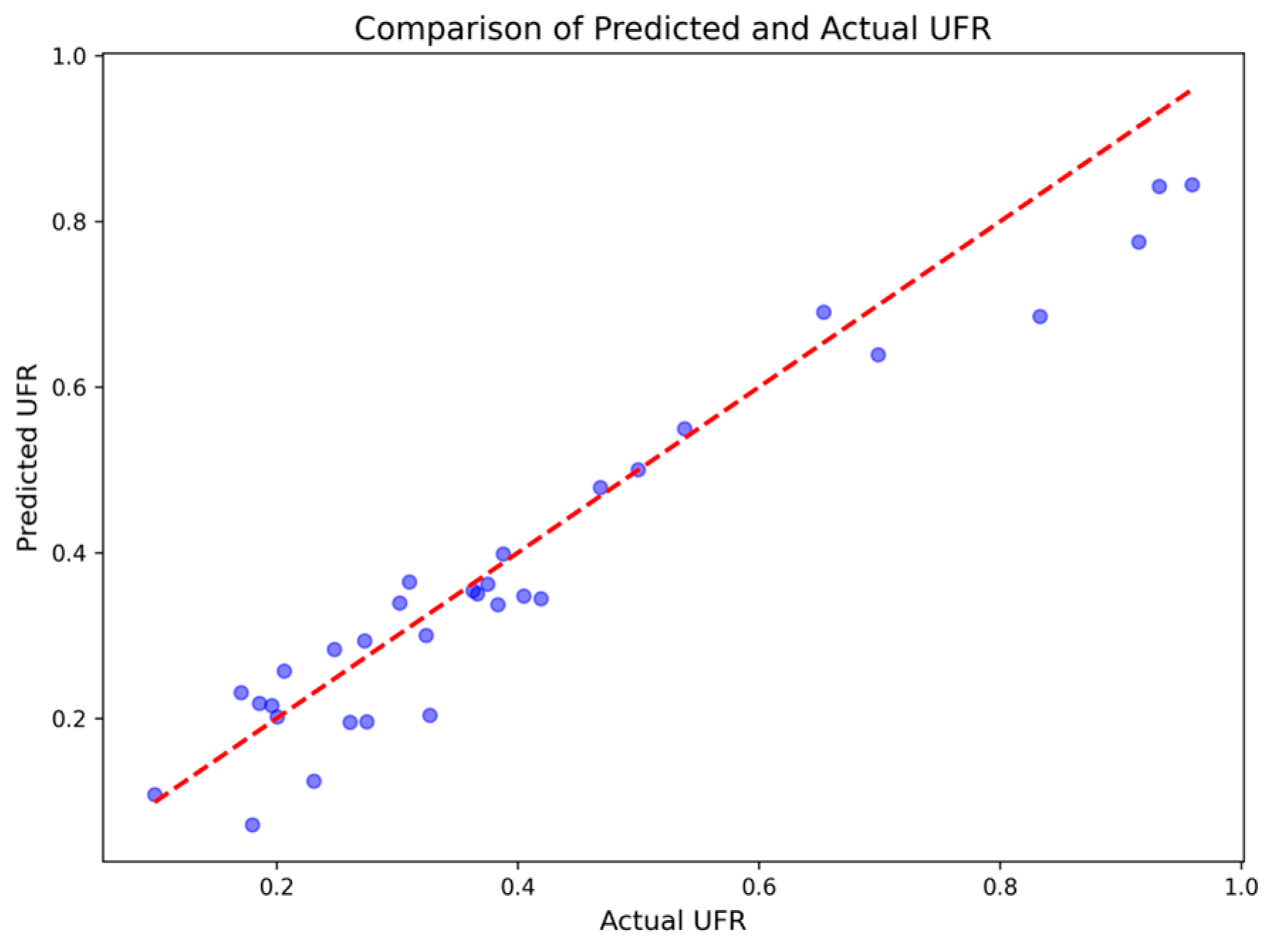
Figure 6 shows a comparison between the model’s predicted UFR values and the actual values. The blue points represent the predicted and actual values for each city, while the red dashed line represents the ideal perfect prediction line. Most of the points are close to the diagonal, indicating that the model’s predictions are generally accurate, though a few points deviate from the line, suggesting prediction errors in certain cities or years. Overall, the model can accurately predict UFR values in most cases.

To ensure the model’s generalizability, overfitting is controlled by applying regularization (L1 = 0.27, L2 = 0.06) and early stopping techniques. This study compares the performance of Random Forest, GBDT, and XGBoost models. The test results indicate that the XGBoost model outperforms both the GBDT and Random Forest models in terms of various loss functions, including $R^2$ (coefficient of determination), MAE (Mean Absolute Error), MSE (Mean Squared Error), and RMSE (Root Mean Squared Error), as shown in

Table 4. Model performance comparison.

Model	Train R2	Test R2	Train MAE	Test MAE	Train MSE	Test MSE	Train RMSE	Test RMSE
XGBoost	0.9898	0.9618	0.0169	0.0347	0.0004	0.0021	0.0216	0.0454
GBDT	0.9852	0.8925	0.0012	0.0382	0.0002	0.0058	0.0015	0.0762
Random Forest	0.9813	0.8601	0.0151	0.0455	0.0004	0.0075	0.0200	0.0869

. Notably, the $R^2$ value on the test set is close to 0.9618, demonstrating the excellent predictive performance of the model. Therefore, XGBoost was selected as the final predictive model, and the SHAP framework was further employed to interpret feature contributions and driving mechanisms of UFR. The optimal parameter combination was ultimately determined to be: n_estimators = 1014, max_depth = 5, subsample = 0.8, colsample_bytree = 0.8, and learning_rate = 0.02.

4.1.2. Analysis of Driving Indicators Based on the SHAP Model

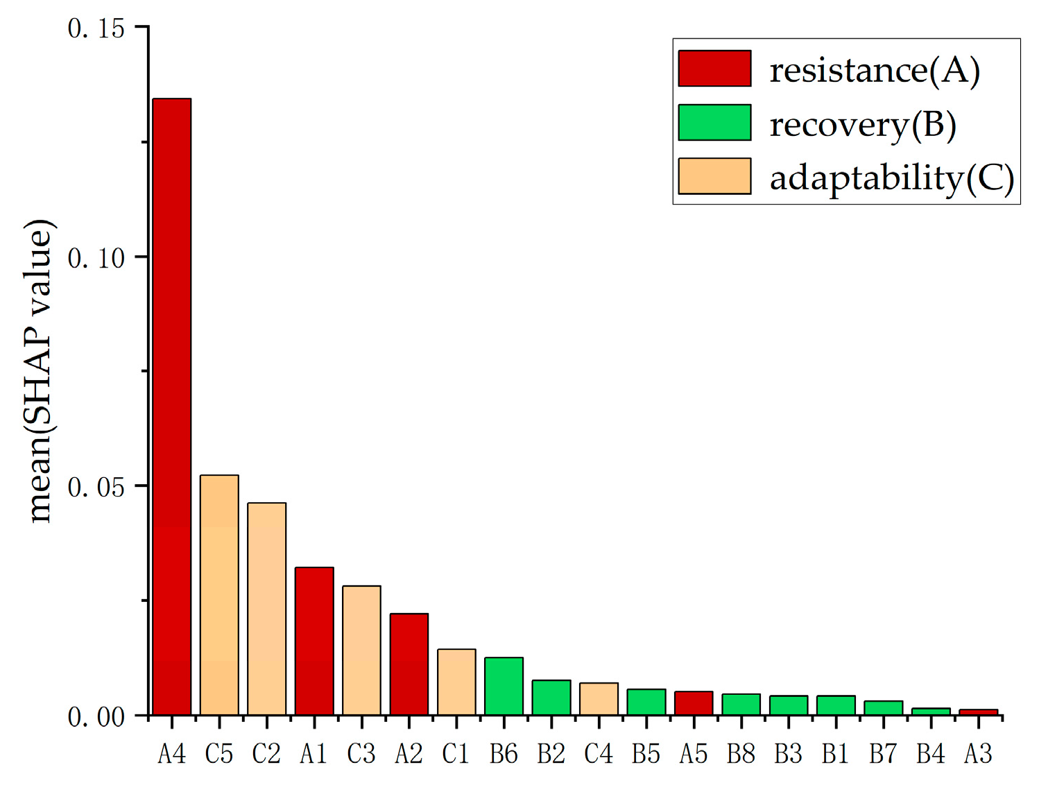
Figure 7 shows the SHAP feature importance plot, which indicates the contribution of each feature to the model’s predictions. Feature importance is determined by calculating the average SHAP value of each feature in relation to the model’s prediction outcomes. Features with higher importance contribute more to the model’s predictions, and this ranking helps identify the key indicators driving UFR.

As shown in Figure 7, six indicators—average urban slope, hydrological station density, per capita park green space area, urban population density, R&D expenditure as a percentage of GDP, and green coverage ratio in built-up areas—have contributions exceeding 0.02. This suggests that these indicators have a high level of impact on UFR, making them critical drivers of UFR in the region.

The indicators related to flood prevention and disaster mitigation policies, tertiary sector value added as a share of GDP, health technicians, per capita public budget expenditure, per capita disposable income, and drainage pipeline density contribute between 0.005 and 0.02 to the average SHAP value, indicating a moderate effect on UFR. Indicators such as wastewater treatment rate, health insurance coverage, urban unemployment rate, urban road area, vulnerable community groups, and precipitation contribute less than 0.005 to the average SHAP value, indicating a relatively weak impact on UFR.

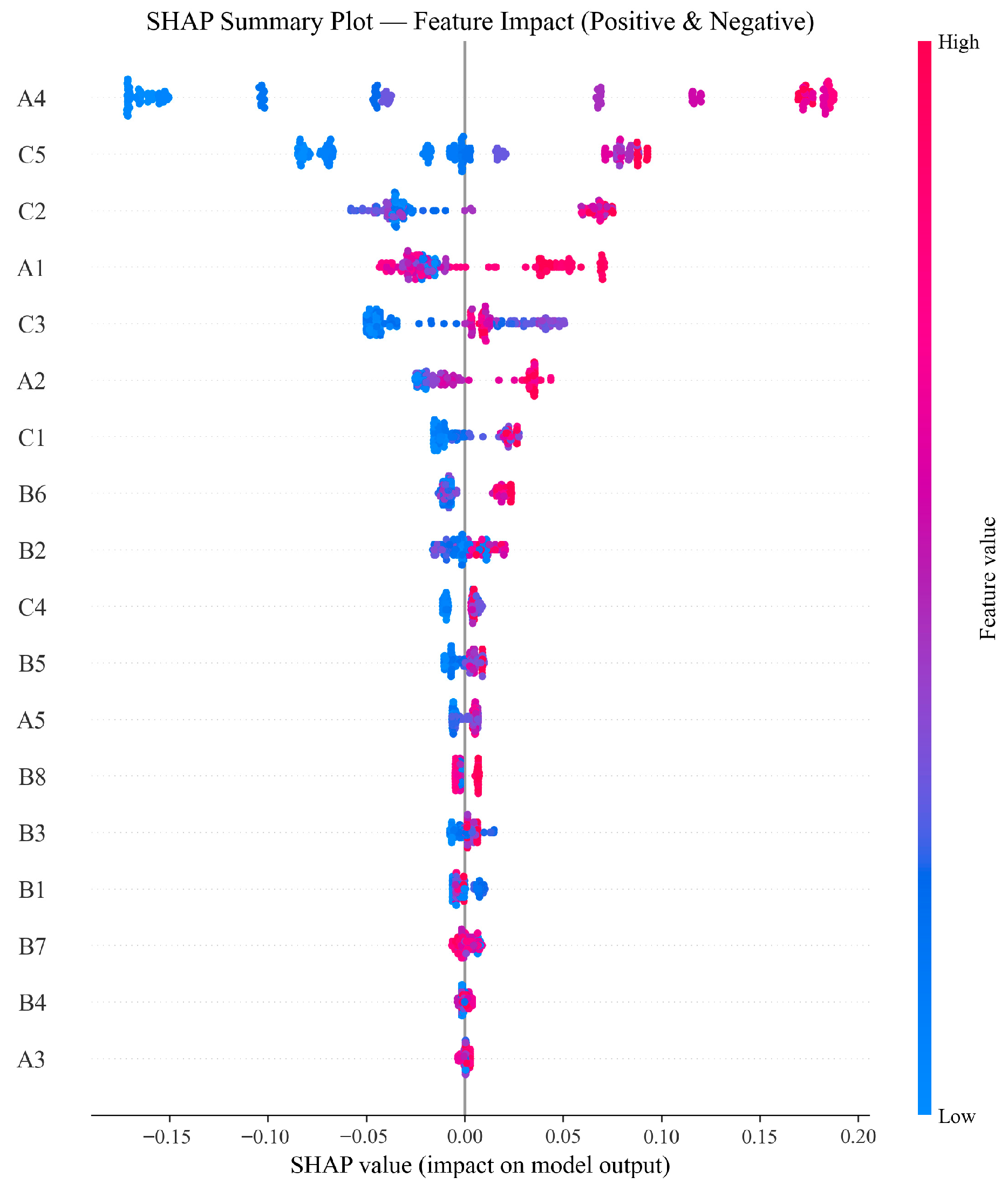
Figure 8 shows the positive and negative impacts of each feature on the prediction results at different value levels. The horizontal axis represents the SHAP values, with each point representing a sample; the color gradient from blue to red indicates the feature values ranging from low to high.

The following conclusions can be drawn from Figure 8; urban slope exhibits a clear positive driving effect: higher values are mainly concentrated in the positive SHAP value range, while lower values are predominantly found in the negative range. This suggests that an increase in urban slope significantly enhances resilience, while a decrease suppresses it. Hydrological station density, per capita park green space area, urban population density, R&D expenditure as a percentage of GDP, and green coverage ratio show a similar distribution pattern to urban slope, making them key drivers of resilience improvement. Flood prevention and disaster mitigation policies, tertiary-sector value added as a share of GDP, health technicians, per capita public budget expenditure, per capita disposable income, drainage pipeline density, and the proportion of vulnerable groups also primarily exhibit higher values in the positive range and lower values in the negative range. However, their points are closer to the zero value, indicating a relatively smaller impact, making them secondary features that contribute positively to resilience. Urban registered unemployment rate shows that high-value samples are mostly distributed in the negative SHAP value range, while low-value samples are biased toward the positive SHAP value range. This suggests that an increase in the unemployment rate reduces resilience, while smaller values help enhance it. Wastewater treatment rate, health insurance coverage, per capita urban road area, and precipitation are distributed on both sides of zero, with samples from high and low values scattered across the positive and negative ranges, showing no clear positive or negative feedback effects.

In summary, Figure 8 not only clarifies the direction and nonlinear impact of each feature but also aligns with the importance ranking from Figure 7. From a policy perspective, resources should be allocated toward the key positive indicators, particularly those with a higher SHAP value, such as urban slope and green coverage. Furthermore, targeted management strategies should focus on constraint indicators, such as the unemployment rate, to improve overall resilience.

4.1.3. Strategies for Improving UFR

Building upon the findings presented in Section 4.1.2, future urban planning should focus on developing indicators related to resistance and adaptability to maximize UFR. Key recommendations include:

Managing population growth: Areas with higher population density tend to have lower UFR, highlighting the importance of controlling urban sprawl and maintaining sustainable population levels.

Integrating ecological considerations: Urban areas with more green infrastructure, such as parks and vegetation, show better flood resilience. Increasing green infrastructure, enhancing soil permeability, and reducing surface runoff through permeable surfaces and green spaces are essential steps.

Strengthening monitoring and management: Cities with robust hydrological systems have better flood response capabilities. Expanding hydrological stations, improving flood forecasting, and enhancing data collection are critical for strengthening adaptive capacity.

Increasing R&D funding: Technological advancements in flood risk management are crucial for developing better flood-resistant infrastructure. Investing in R&D will support this progress.

Implementing these strategies will help cities adapt to urban and environmental challenges, as demonstrated by the flood adaptability planning in Seoul’s Gangnam District, where green infrastructure plays a key role in sustainable urban design and planning [40].

4.2. Advantages of the Proposed Method

Firstly, a UFR index system covering four dimensions was established through a review of relevant literature. This system integrates indicators from natural, economic, social, and infrastructure aspects, providing a comprehensive research framework. Additionally, the evolution of resistance, recovery, and adaptability aligns with the cyclical nature of urban systems.

Furthermore, compared to traditional methods such as the obstacle degree model, the XGBoost-SHAP method combines the efficiency of machine learning with strong interpretability. This approach not only improves prediction accuracy when handling complex urban flood resilience drivers but also effectively reveals the quantitative contributions and directional impacts of each factor.

4.3. Limitations and Future Research Directions

This study provides valuable insights into UFR in the BTH region but acknowledges the limitations of the multi-method coupling approach. The combination of CRITIC-Entropy, VIKOR, and XGBoost-SHAP offers a comprehensive framework for UFR assessment, but each method has its own assumptions and limitations. For instance, CRITIC, based on linear correlations, may not capture the complex nonlinear relationships between indicators. Although VIKOR and entropy weighting improve upon this, they remain influenced by data distribution, limiting their ability to account for dynamic interactions across resilience dimensions. Therefore, while the multi-method approach is effective, its limitations in capturing UFR dynamics should be considered.

Additionally, the absence of explicit flood modeling is a key limitation. While non-hydrological data provide valuable insights, integrating hydrological simulations or watershed models would offer a more accurate representation of flood risks, especially during extreme weather events. Future research could explore integrating flood modeling to enhance the reliability of UFR assessments.

The data used in this study also has limitations, particularly in terms of adaptability. Adaptability, representing the ability of urban systems to achieve sustainable development through learning and adjustment, was not fully captured due to data constraints, especially socio-institutional factors such as community preparedness and governance quality. Future studies should incorporate these factors. Furthermore, rainfall variability presents challenges for flood resilience assessments. More refined rainfall metrics, such as IDF curves or maximum hourly rainfall, should be considered to reflect flood risks more accurately.

Meanwhile, future research could enhance UFR assessments by conducting quantitative validation using actual flood loss data, helping to verify the effectiveness of the current model. Sensitivity and uncertainty analyses would also reveal the impact of different variables and methods on the results, leading to more reliable outcomes.

Finally, flood risks often extend across administrative boundaries. Using administrative boundaries for flood resilience assessment may lead to inaccurate results. Future research should explore ways to overcome these constraints and promote data sharing and coordinated planning across regions.

4.4. Validation of MCDM Models

To ensure the robustness and reliability of the MCDM models used in this study, we conducted a validation. We focused on two widely used methods: VIKOR and TOPSIS. We compared these two methods in terms of their ability to rank cities based on UFR.

We calculated Kendall’s Tau for each city, with a coefficient of 0.4862, indicating a moderate positive correlation between the rankings derived from VIKOR and TOPSIS methods. The p-value of 2.11 × 10⁻¹⁹ confirmed that this correlation is statistically significant, further strengthening the consistency and reliability of both methods.

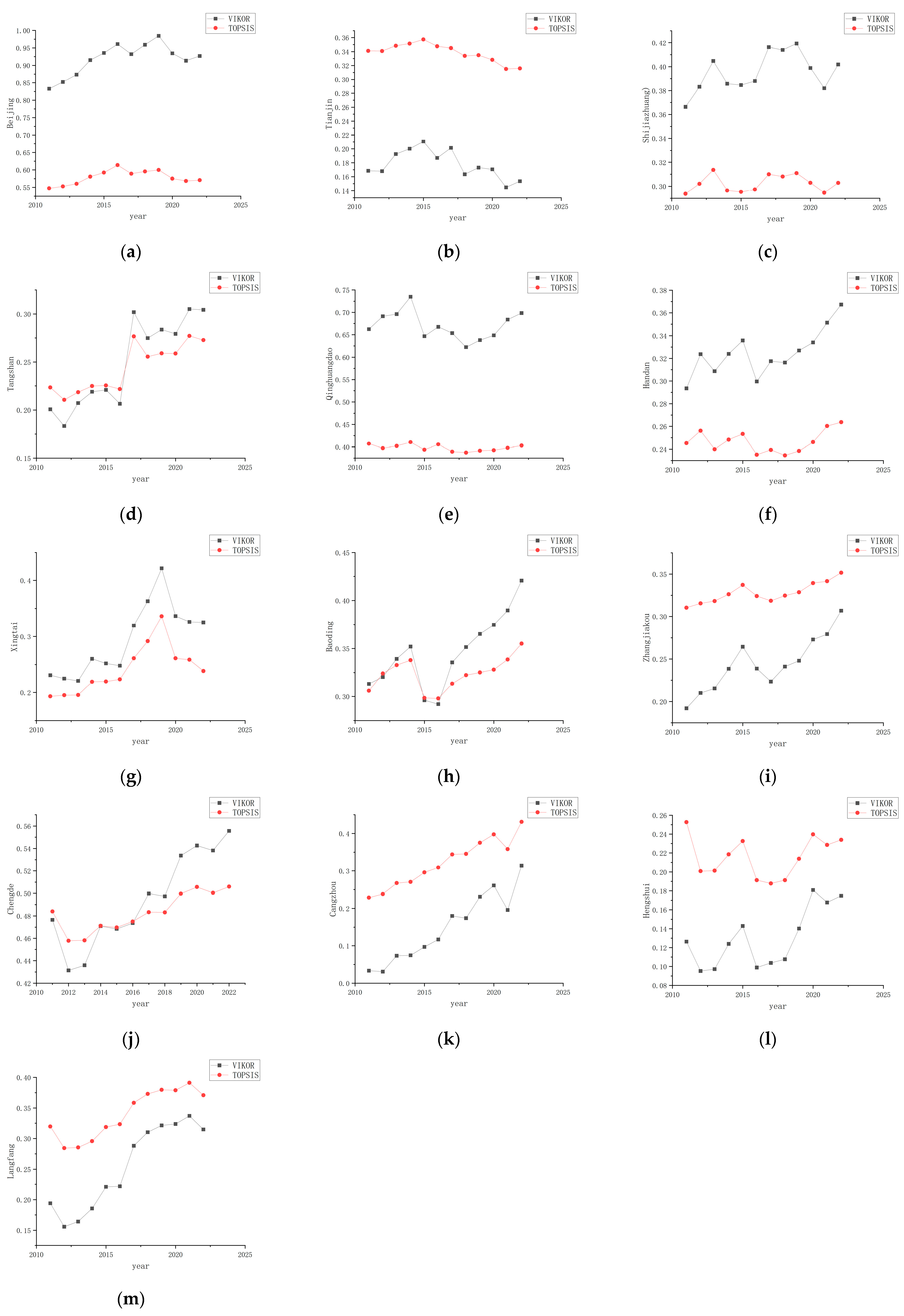
From the comparison of the line charts for all cities from 2011 to 2022, as shown in Figure 9, it is evident that the VIKOR curve shows a wider interval, stronger inter-annual monotonicity, and no intersections between cities, significantly outperforming the low distinguishability of TOPSIS. VIKOR demonstrates higher sensitivity and is better at capturing the fluctuating changes in UFR.

5. Conclusions

This study proposed an evaluation framework of UFR, and then the spatiotemporal evolution and attribution of UFR of the BTH region from 2011 to 2022 was assessed across the three dimensions of resistance, recovery, and adaptability.

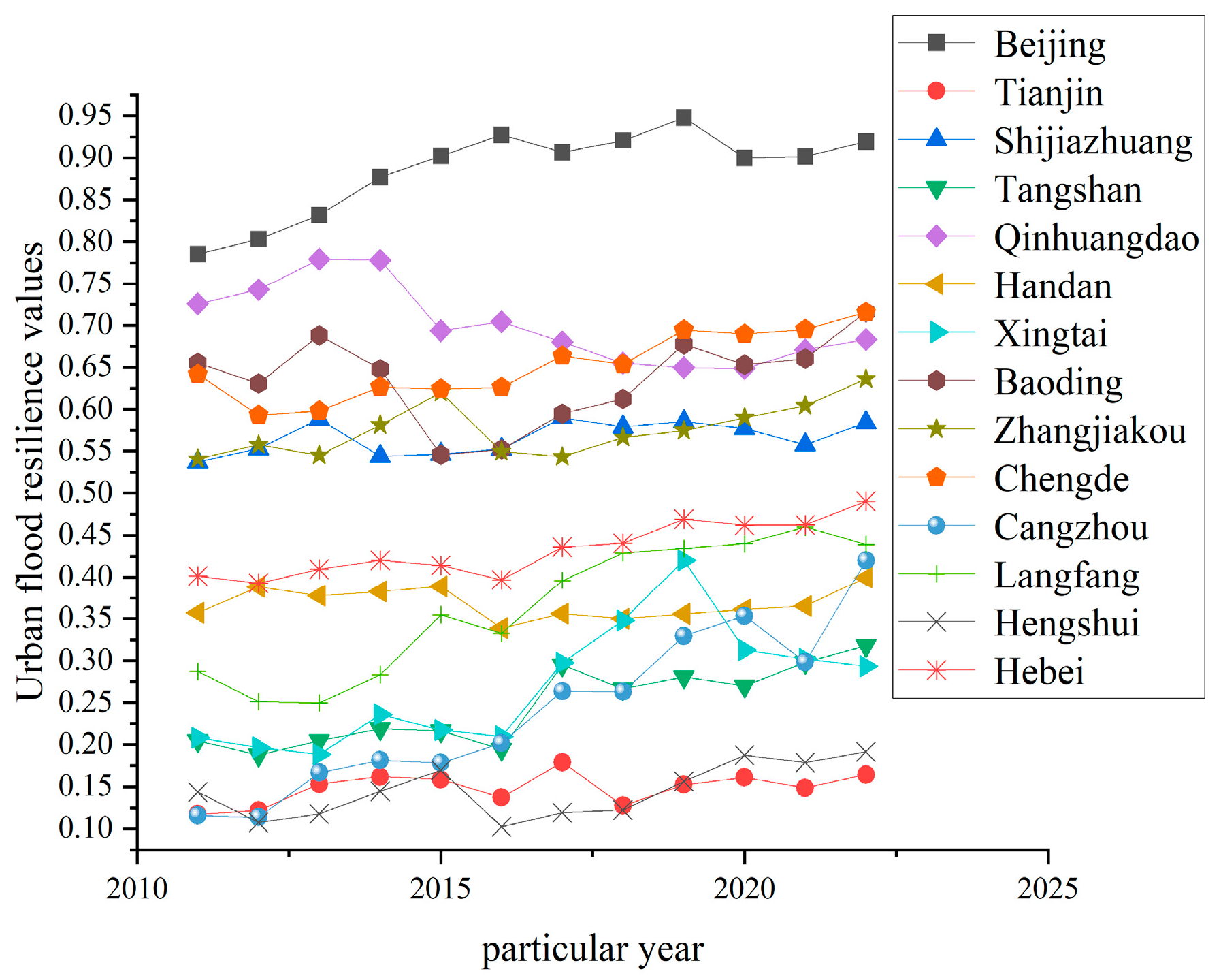
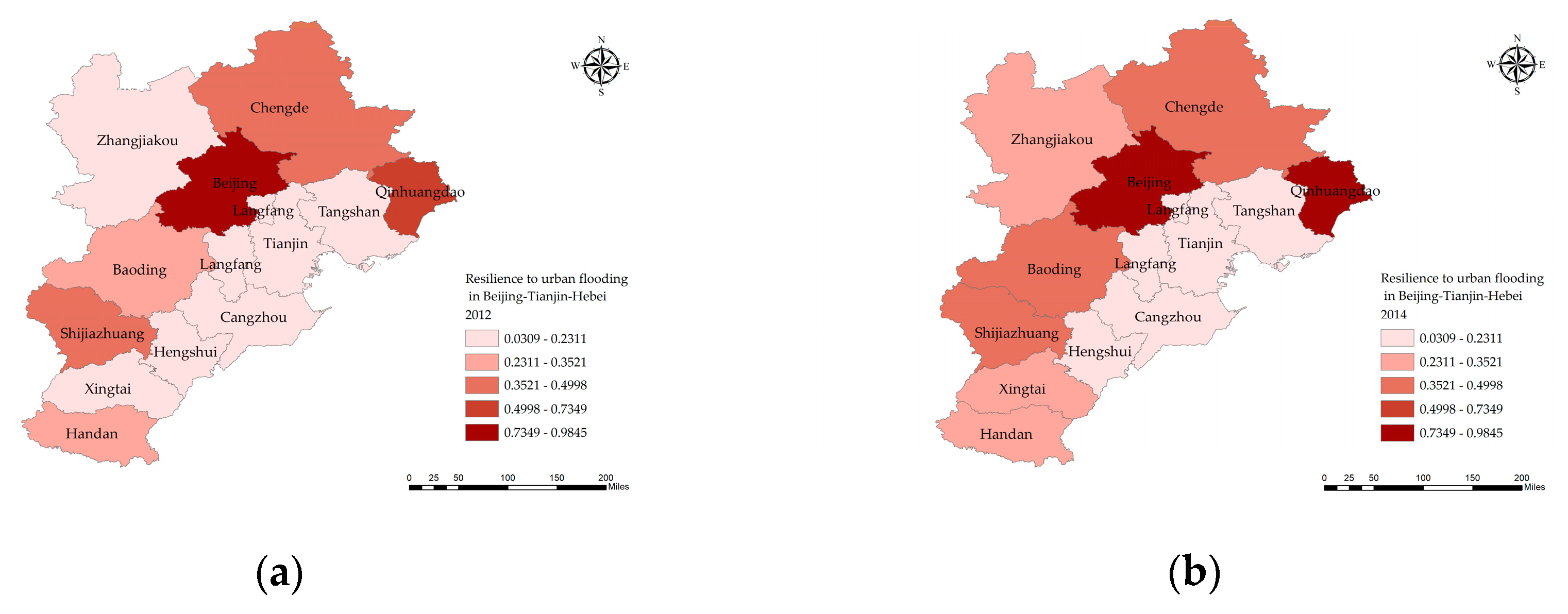
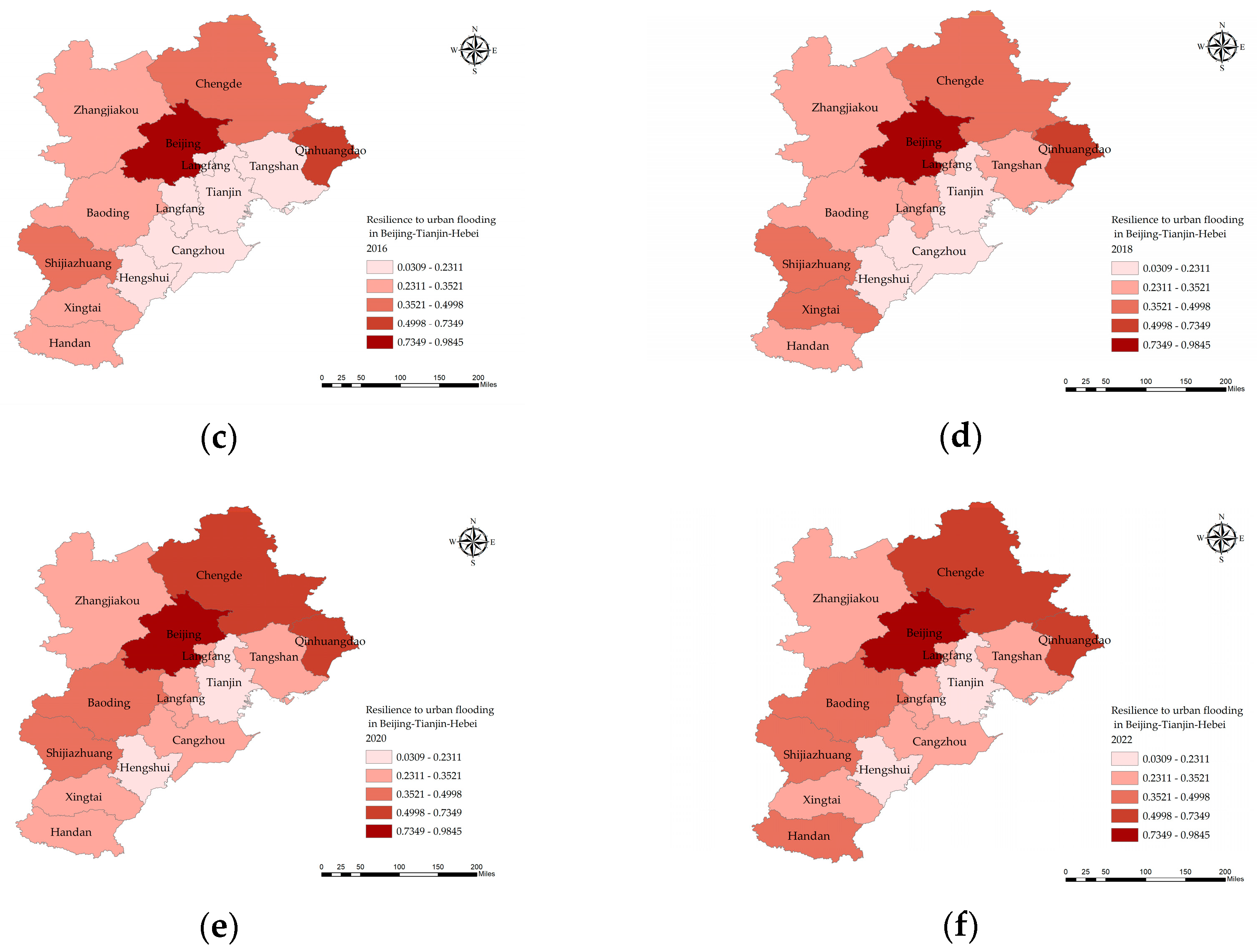
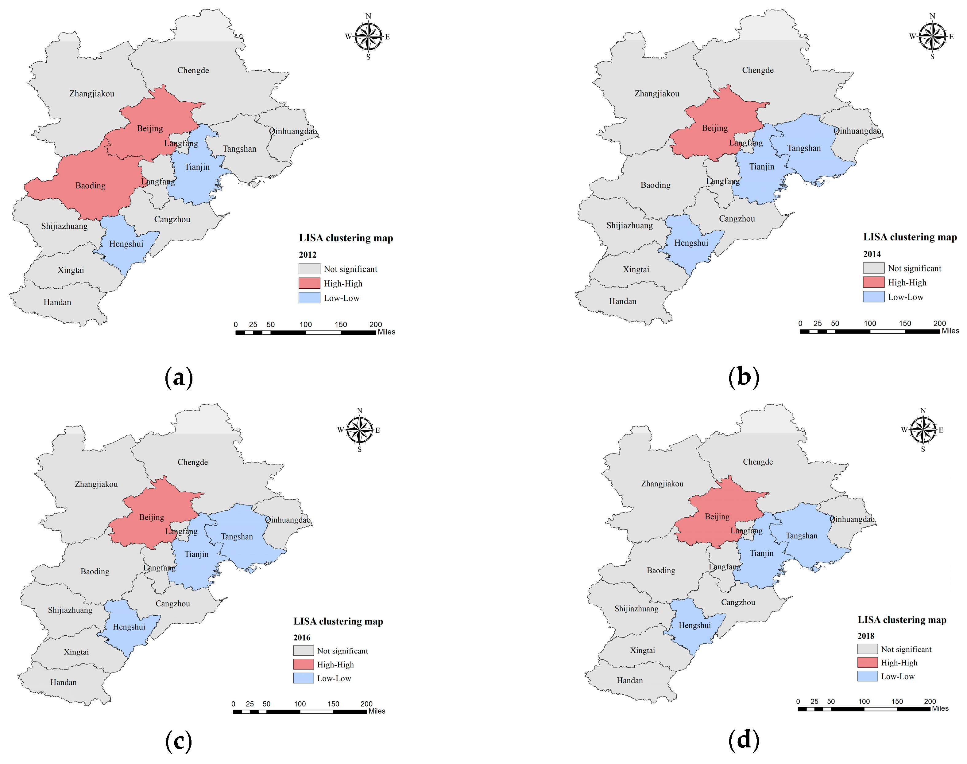
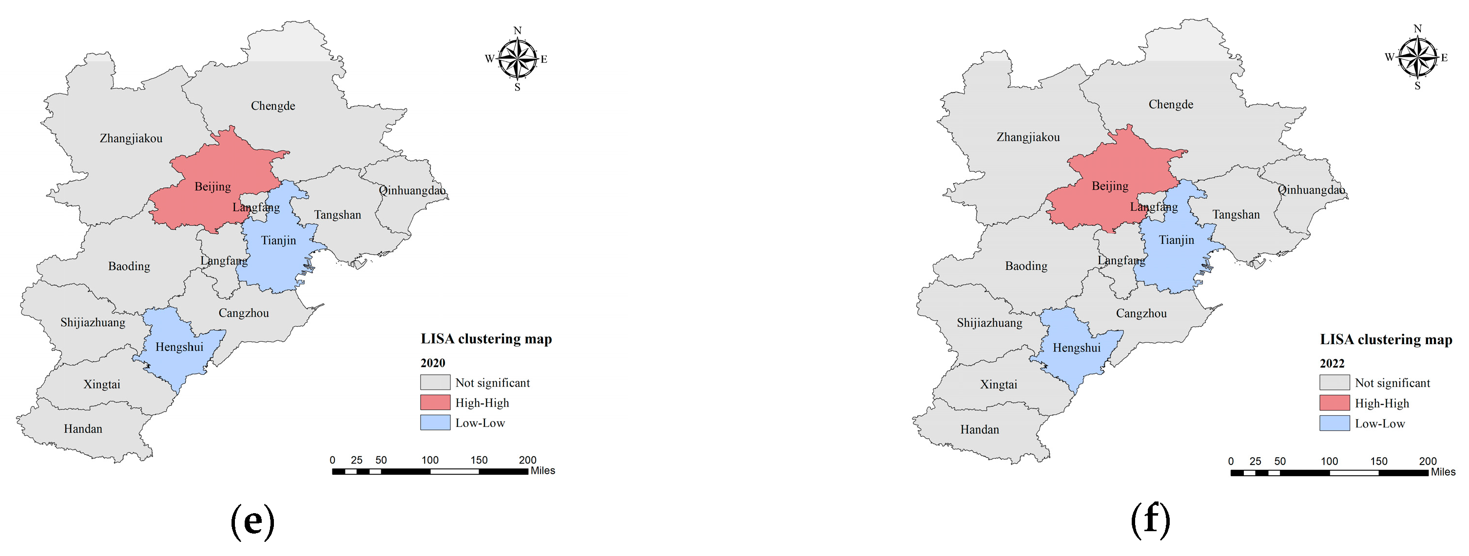
The results reveal that the overall UFR in the BTH region exhibited a fluctuating but upward trajectory, indicating gradual improvements in regional resilience capacity. Beijing consistently maintained the highest resilience level, the resilience values are all above the critical threshold of 0.7349, which can be largely attributed to its favorable geographic and socio-economic advantages. Spatially, a distinct gradient pattern was observed, characterized by higher resilience in the northwest and lower resilience in the southeast. Notably, the number of cities classified as low or very low resilience declined over time, while the disparity in resilience levels across cities narrowed under the influence of regional coordinated development policies. Spatial autocorrelation analysis further revealed clustering effects, with high-value clusters centered around Beijing and low-value clusters concentrated in Tianjin.

The decomposition analysis highlights that indicators related to resistance and adaptability, such as urban slope, hydrological station density, per capita urban park area, urban population density, the proportion of R&D expenditure to GDP, and green coverage in built-up areas, were the primary drivers of resilience enhancement during the study period. In contrast, the urban registered unemployment rate was found to have a marginal inhibitory effect, hindering the overall improvement in UFR.

Given the hydrological complexity of the BTH region, the findings of this study are primarily applicable to this region but could also be extended to other cities facing similar challenges, such as those with high population density and rapid urbanization. These results offer valuable guidance for urban planning and policy-making, helping cities better prepare for future flood risks.

Collectively, these findings provide a scientific basis for guiding policy formulation and urban planning aimed at strengthening urban flood resilience and ensuring sustainable urban development in the face of increasing hydrometeorological risks.