Mapping and Assessing Groundwater Quality in Bourgogne-Franche-Comté (France): Toward Optimized Monitoring and Management of Groundwater Resource

Abstract

To optimize the management of groundwater resources in the Bourgogne-Franche-Comté (BFC, France) region, data from the Size-Eaux database were cross-referenced with the French Reference Framework for Groundwater Bodies (GWB). The information contained in this dataset was synthesized using Principal Component Analysis (PCA), followed by Agglomerative Hierarchical Clustering (AHC) of GWBs based on their average coordinates along the main factorial axes. The results reveal 11 distinct GWB groups, each internally homogeneous in terms of chemical composition and ongoing processes responsible for intra-group variability. The distribution of the groups aligns with the region’s structural geology, lithology, and agricultural activity patterns. Livestock farming areas, prone to fecal contamination, and cereal-growing areas, characterized by high nitrate concentrations, stand out distinctly. Furthermore, the analysis of GWB groups highlights regional processes such as denitrification, confirming the existence of spatial structuring of these mechanisms beyond local specificities. The major physicochemical and bacteriological zones show strong contrasts between groups while maintaining significant internal homogeneity. Despite the region’s vast size and diversity, spanning three major watersheds, further subdivision was not necessary to obtain applicable results. These findings confirm observations made in other regions and pave the way for an optimized monitoring and surveillance strategy.

1. Introduction

Groundwater aquifers, less vulnerable to pollution than surface waters, play a crucial role in supplying drinking water to populations. In the context of increasing pressure on this vital resource [1,2,3,4], protecting it from contamination requires identifying the most exposed or vulnerable areas and conducting an in-depth analysis of the mechanisms responsible for spatiotemporal variations in water quality. The chemical and bacteriological composition of groundwater provides valuable information by recording what happens on the surface (livestock farming and agricultural or urban pollution), during its passage through soils (filtration or lack thereof, variations in CO₂ partial pressure and organic carbon, and the impact of soil bacteria), and during deep circulation within the geological formations that contain it (water–rock interactions) [5,6,7]. The physicochemical and biological characteristics of water are commonly used as natural indicators or tracers in the study of water transfers. This approach relies on the stability of these signatures over time, as well as their spatial distribution within water bodies. However, it is essential to recognize that the underlying mechanisms of water quality vary depending on lithology, land use, and anthropogenic impacts. At the regional scale, where lithology can become heterogeneous, upscaling study areas becomes problematic, compromising the effective use of natural indicators or tracers [8]. Thus, managing the heterogeneity of geological characteristics when scaling up from local to regional levels is of critical scientific interest in resource management.

Given the complexity of these mechanisms, the scientific literature offers a variety of approaches to address these challenges, covering diverse spatial scales. These methods range from local studies of groundwater abstraction points (e.g., through sentinel or monitoring boreholes) to the analysis of watersheds or groundwater bodies, often characterized by low geological complexity, and even to the regional scale, where geological, altitudinal, and land-use diversity is more pronounced. Methodologies used to identify pollution sources or “non-compliances” include geochemical and multivariate statistical analyses [9], end-member mixing models [10], geostatistical techniques for studying geochemical structures, and modeling at various scales [11,12,13,14,15]. These tools help better understand aquifer dynamics and propose management strategies tailored to their protection.

The present work is part of a series of studies conducted in France, based on the integration of two databases [16,17,18,19,20]. The overarching goal is to clarify the diversity of processes influencing water quality, study the sources of compositional variability, and provide a methodological tool adapted for optimal resource management. The first is the national Sise-Eaux database [21,22], which compiles the physicochemical and bacteriological characteristics of water, maintained by Regional Health Agencies as part of health monitoring since the 1990s. The second is the national reference framework for groundwater bodies (GWB), i.e., a geographical delineation of aquifers conducted by the French Geological Survey (BRGM). These efforts aim to optimize the monitoring and surveillance of groundwater resources. They result in grouping groundwater bodies based on their physicochemical and bacteriological similarities, as well as the processes driving diversity at the regional scale. Since GWB groups are established based on degrees of similarity across all parameters, it is necessary to evaluate the grouping procedure in terms of intra-group similarity and inter-group dissimilarity. Finally, it is essential to characterize each group and study the processes specific to each responsible for water diversity and major non-compliance [23,24,25].

To illustrate the practical application of this methodological framework, the procedure is applied to the Bourgogne-Franche-Comté region, a more continental area spanning three major river basins: The Seine, the Loire, and the Rhône. It will be necessary to verify whether the size of the region and its configuration pose an obstacle to the establishment of a grouping of groundwater bodies (GWB), and more broadly to the application of the method, as has been observed in the Occitanie region [18]. This case study will test the robustness of the approach in a complex geological and hydrological context, providing insights for future applications in other regions with similar challenges.

2. Materials and Methods

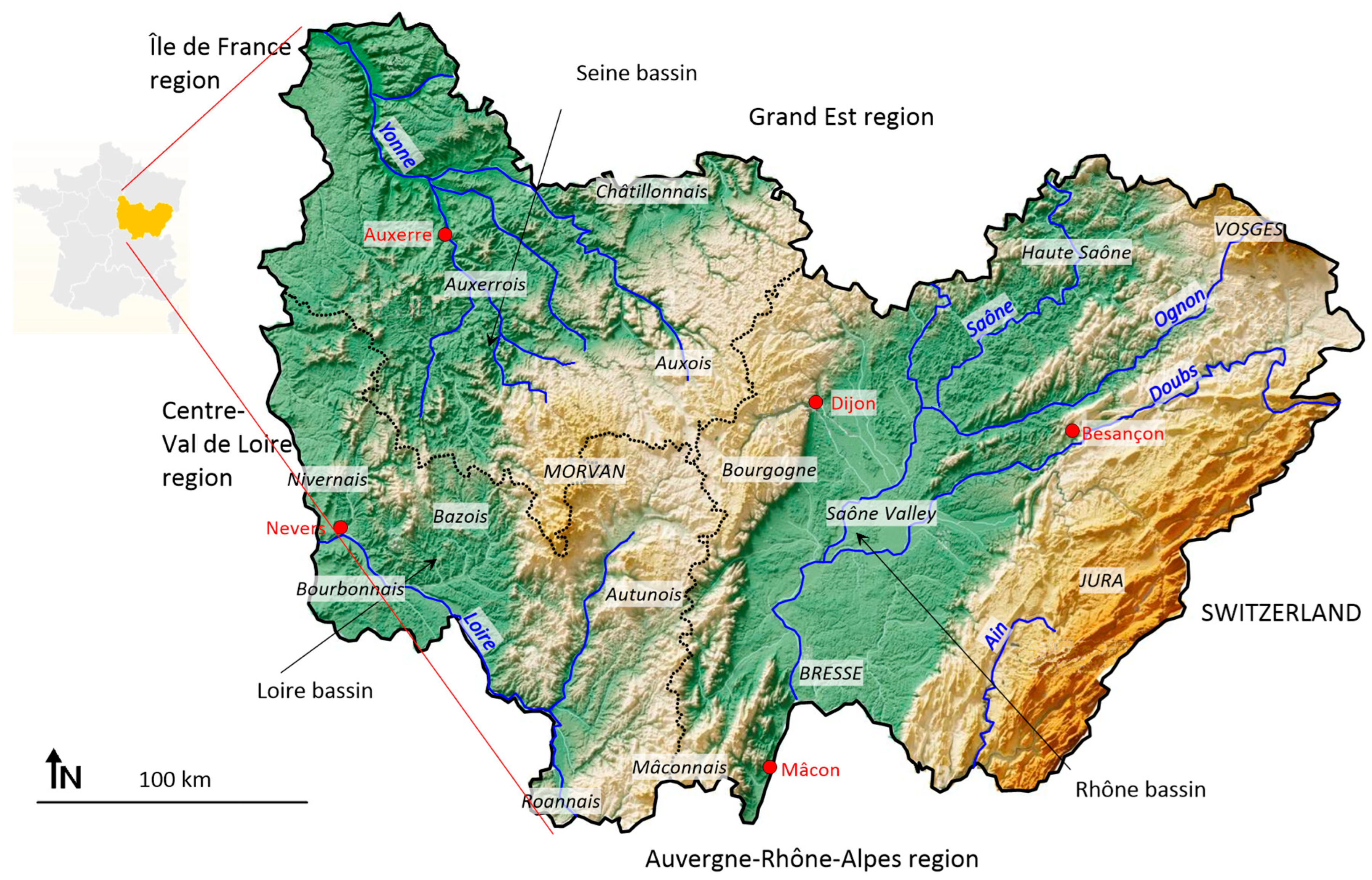
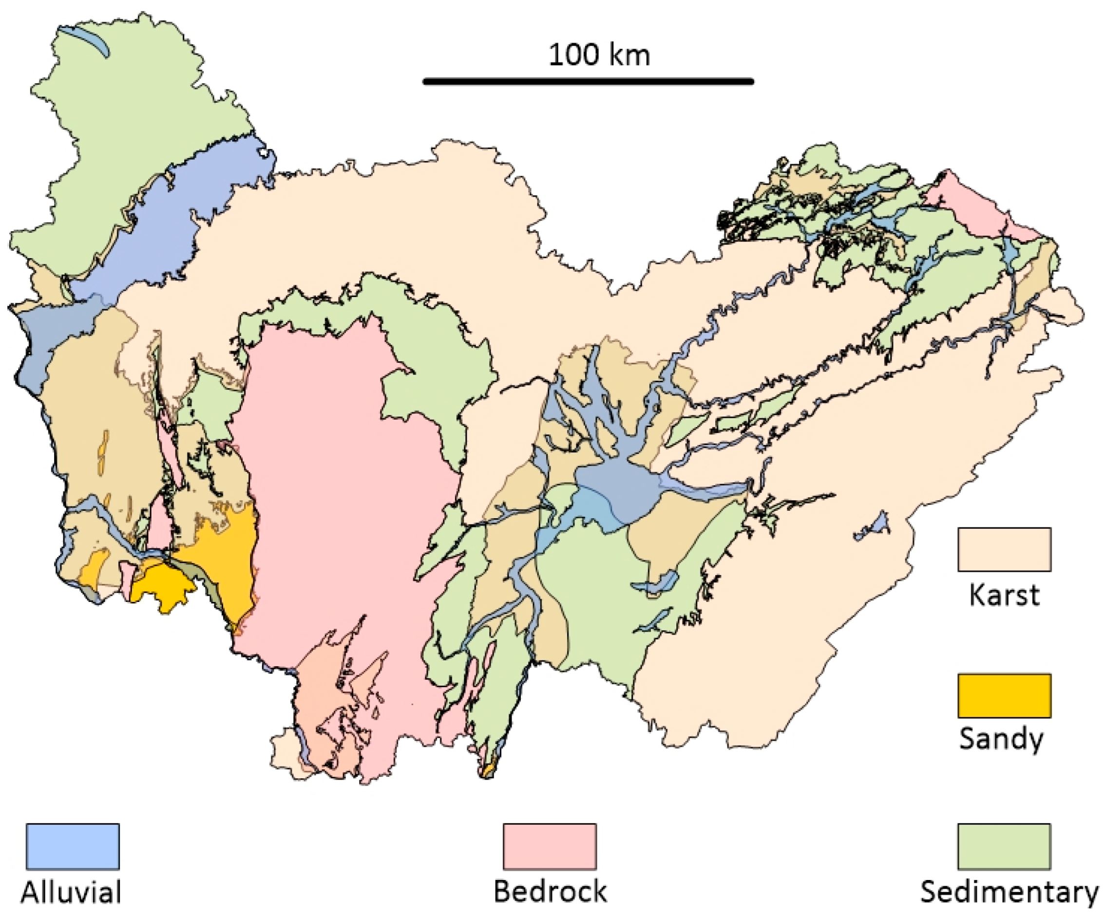
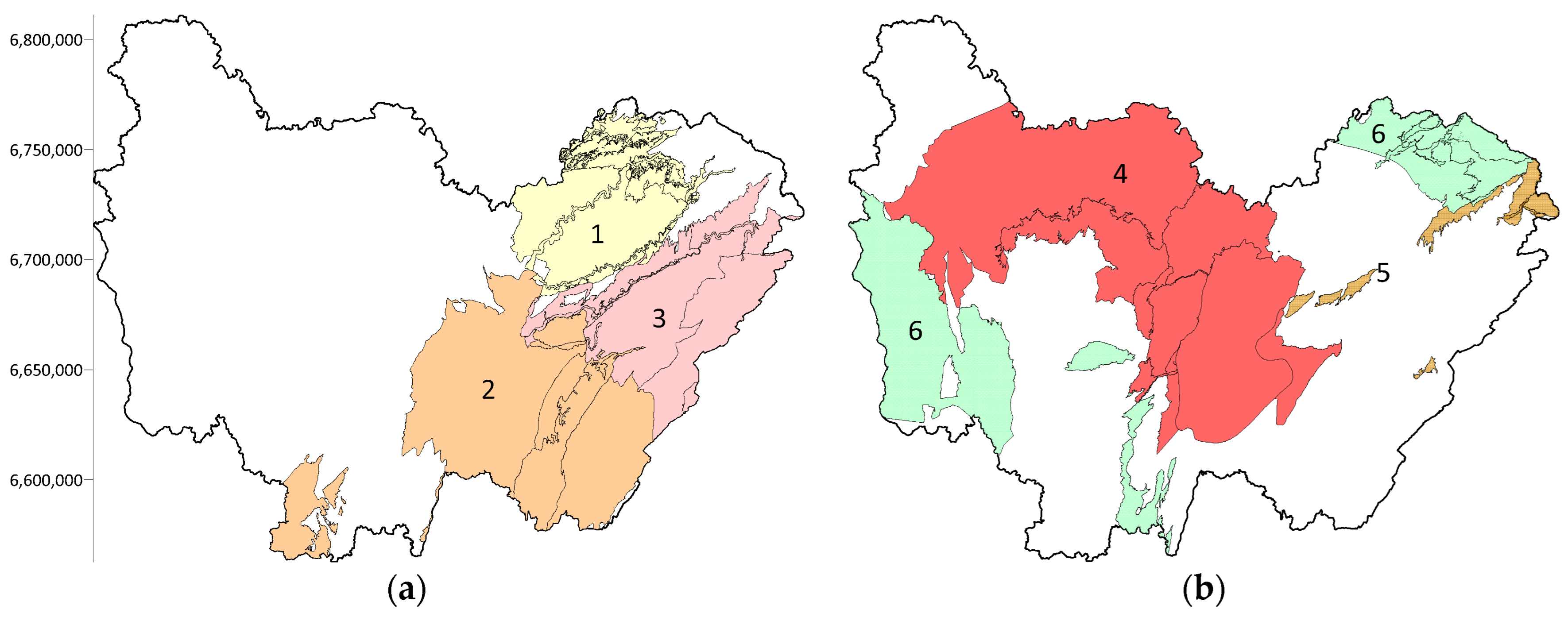
2.1. Study Site: Bourgogne-Franche-Comté Region

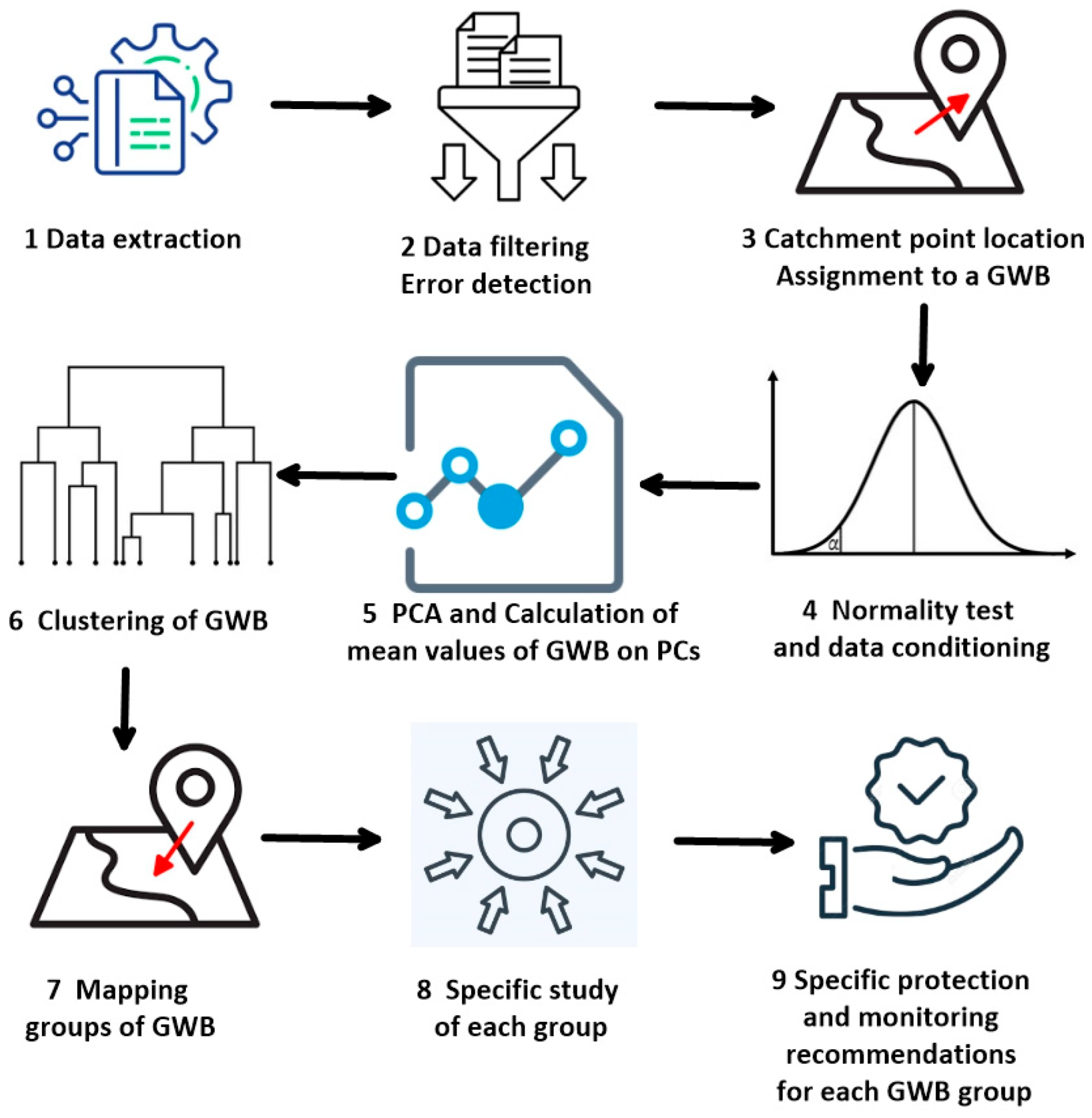
The Bourgogne-Franche-Comté (BFC) region, located in east-central France, covers an area of approximately 48,000 km², making it the fifth largest region in metropolitan France (Figure 1). It is characterized by significant geological diversity, including limestone formations from the Jura, granites and gneisses from the Morvan, and sedimentary basins (Paris Basin, Bresse Graben). For a more detailed presentation of the region, the reader may refer to previous studies [26]. This lithological heterogeneity strongly influences groundwater quality, with aquifers exhibiting varied hydrogeological properties in terms of porosity, permeability, and vulnerability to contamination. A breakdown of the main aquifer types is provided in Figure 2. The region also features contrasting land use, ranging from intensive beef farming in the Morvan and dairy farming in the Jura to large-scale cereal cropping in the plains.

2.2. Databases

Under the impetus of the European Water Framework Directive (WFD) in 2000 [27,28], the Water Agencies, with the support of the French Geological Survey (BRGM), undertook the inventory of groundwater reservoirs at the national level (https://services.sandre.eaufrance.fr/geo/sandre, accessed in 6 February 2023). These reservoirs were subdivided into groundwater bodies (GWBs) and their boundaries were delineated and geolocated to be included in the Water Information System for Europe (WISE) [29,30]. By definition, a GWB represents a distinct volume of groundwater located in one or more aquifers, which are composed of geological layers with sufficient porosity and permeability to allow either significant groundwater flow or exploitation. At the national level, these GWBs are identified by a unique code consisting of the abbreviation FR for France, a letter X designating the main river basin (in our case, D for Rhône, H for Seine, and G for Loire), and the letter G designating the groundwater resource. Thus, GWBs are referenced from FRXG001 to FRXG999. In total, 70 GWBs have been identified in the Bourgogne-Franche-Comté region. This number is too high to define an analysis of the processes influencing the water quality of each GWB, but it provides an essential basis for identifying homogeneous groups on which to develop tailored monitoring and surveillance policies.

Alongside the GWB reference framework, the physicochemical and bacteriological characteristics of the water were extracted from the Sise-Eaux database (https://data.ofb.fr/catalogue/data-eaufrance/eng/catalog.search#/home, accessed on 15 March 2023), resulting in a full matrix (without missing data) of 3569 observations and 22 parameters, distributed across 989 catchment points (Figure 3). The 22 parameters are electrical conductivity at 25 °C (EC), fecal bacteriology indicators (Enterococcus and Escherichia coli, labeled as Enter. and E.coli), major ions (Na⁺, Ca²⁺, Mg²⁺, Cl⁻, SO₄²⁻, HCO₃⁻, NO₃⁻, and NH₄⁺), metals and trace elements (Fe, Mn, B, F, As, Se, Cd, and Ni), total organic carbon (TOC), and turbidity (Turb.). In the following, a distinction will be made between the parameter and the element or ion measured. For example, SO₄ represents the variable based on the values of SO₄²⁻. For more details on the data extraction process, the reader may refer to previous studies [26,31].

2.3. Obtaining GWB Groups

The methodology for obtaining homogeneous GWB groups includes the following 6 steps:

• Data Conditioning: The data underwent a logarithmic transformation to approximate normal distributions and reduce the influence of extreme values. This conditioning, previously tested on similar datasets from the Occitanie [32], Provence-Alpes-Côte d’Azur [33], Auvergne-Rhône-Alpes [34], and Corsica regions [35], allows for a better analysis of variability sources.
• Sample Assignment: Each of the 3569 samples was assigned to a GWB based on its geographical coordinates and sampling depth.
• Principal Component Analysis (PCA): A PCA was performed on the log-transformed data to reduce the dimensionality of the data space, i.e., eliminate redundancies in the information carried by the parameters, and to identify variability sources [36]. The PCA, conducted by diagonalizing the correlation matrix, considers standardized variables, enabling the integration of parameters with diverse natures and units. Under these conditions, the factorial axes, orthogonal to each other, are associated with independent processes responsible for water quality variability. The first factorial axes, representing approximately 90% of the information contained in the dataset, are retained. The last factorial axes, explaining a small percentage of the variance, are eliminated as they are considered statistical noise.
• Calculation of Averages by GWB: Average values were calculated for each GWB on the retained factorial axes. At this stage, each GWB is characterized by a vector of dimension X, where X is the number of retained factorial axes.
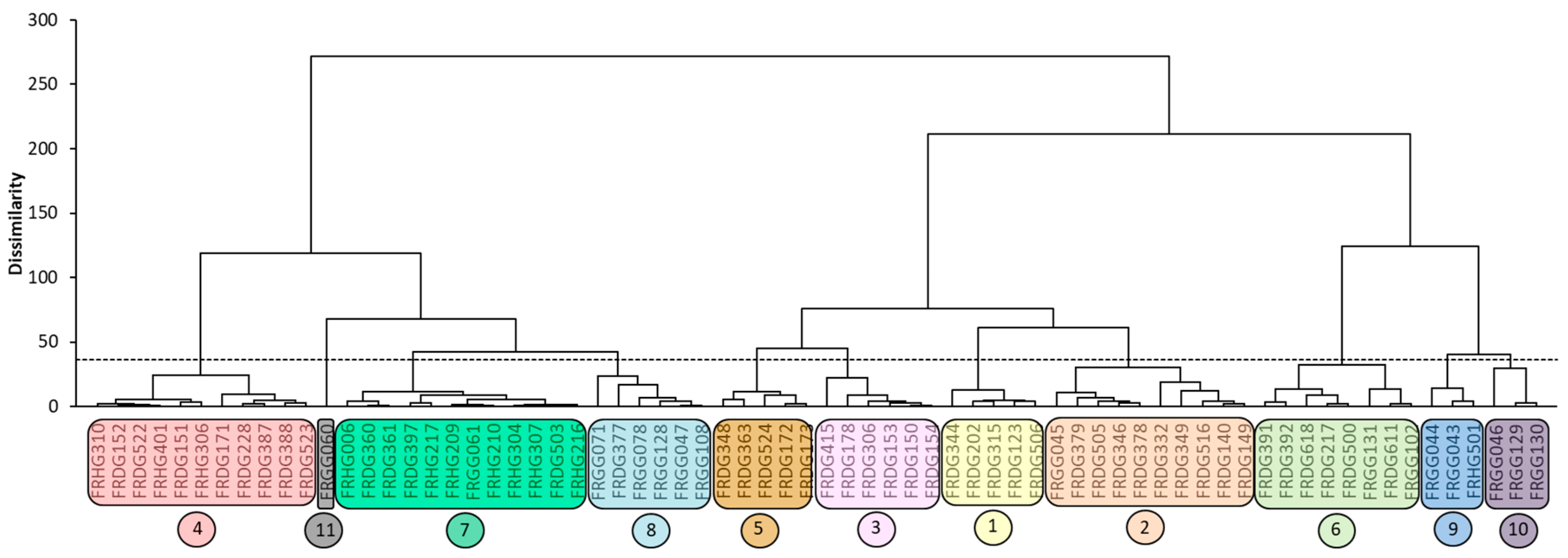
• Agglomerative Hierarchical Clustering (AHC): An unsupervised AHC was applied to group GWBs based on their similarity [37,38,39]. This clustering aims to assemble GWBs into groups according to a similarity criterion in terms of correlation, considering all parameters. The relative similarities between GWBs were quantified using Euclidean distance, and the similarity levels at which GWBs were merged were used to construct a dendrogram. The number of clusters was determined through two guiding principles: 1—practical groundwater management considerations, which typically require between 5 and 15 distinct groups; 2—analysis of the “explained variance percentage vs. number of clusters” curve, where the elbow point (slope break) was selected as it provides the optimal balance between model simplicity (fewer clusters) and information retention (higher explained variance).
• Mapping of GWB Groups: Finally, the GWB groups were mapped in a GIS (Geographic Information System).

2.4. Parameter Classification

To compare the behavior of different parameters, they were grouped using unsupervised hierarchical clustering [39] based on the coordinates of the parameters on the principal factorial axes. This means that the clustering was performed according to the correlation information between the parameters.

2.5. Analysis of GWB Groups and of Clustering Methodology

The average of each parameter for each GWB group was calculated, and the relative positions of each group based on key parameters were analyzed. Additionally, a specific PCA was conducted on the homogeneous GWB groups to identify the main sources of variability. A linear discriminant analysis (LDA) was performed to determine which combination of parameters best discriminated the closest groups and to predict the assignment of water samples to their respective GWB groups [40,41]. The results are based on the confusion matrix and graphically on the ROC (Receiver Operating Characteristic) curve analysis [42]. Then, the results were compared to a similar discrimination using a naïve Bayesian analysis, with 10% to 90% of the dataset used for the training phase [43]. Finally, to test the homogeneity within GWB groups, an analysis of variance (ANOVA) was performed using the R² coefficient to measure, for each parameter, the explained variance at the sampling point scale and at the groundwater body (GWB) scale. The explained variance at the sampling point scale reflects spatial variability at this scale, and the deviation of R² from unity indicates the variance associated with temporal variability, along with a component linked to analytical imprecision considered negligible [44,45].

3. Results

3.1. Groundwater Bodies Grouping

The first 11 principal components, accounting for nearly 91.1% of the information contained in the dataset, were retained for the clustering of GWB. The remaining 8.9%, carried by the next 11 factorial axes, was considered statistical background noise. The clustering of GWB leads to the dendrogram presented in Figure 4, where the placement of the phenom line (dotted line) allowed for the distinction of 11 homogeneous groups.

The distribution of these 11 groups across the region (Figure 5) highlighted the clustering of neighboring GWBs or those belonging to similar geological contexts, emphasizing the coherence of the results. These groups reflected the geological and hydrogeological diversity of the region, notably with Group 9 located in the granitic sector of Morvan and Autunois; Groups 4 (Auxerrois, Châtillonnais, Auxois, and Bourgogne), Group 7 (Yonne Basin and Monts du Mâconnais) associated with sedimentary limestone formations, and Group 1 in the Haute-Saône sector. Groups 2 and 3 corresponded to the southern and northern Jura geographical entities and their influence zone on the Bresse Plain, respectively. Group 5 included the riverin aquifers of the Ognon River, while Group 6 mainly consisted of two distant sectors: the Vosges Massif in the northeast and the Bazois-Nivernais area in the west of the region. Group 8 corresponded to the riverine aquifers of the Saône and Loire rivers. Group 10 was located in the calcareous marl formations of Nivernais, Bourbonnais, and Roannais, and finally, Group 11 consisted of a single GWB in the sandstone and marl formations of Bazois.

The average parameter values for each GWB group are summarized in

Table 1. Average values of each parameter for each GWB group (log values).

Group	EC	E.coli	Enter.	NH4	As	Na	Ca	Mg	Cl	SO4	HCO3
1	2.636	0.668	0.592	−1.175	0.347	0.576	1.861	0.767	0.824	1.112	2.361
2	2.627	0.896	0.769	−1.468	0.271	0.368	1.904	0.443	0.608	0.753	2.391
3	2.678	1.035	0.877	−1.605	0.420	0.539	1.956	0.510	0.776	0.858	2.439
4	2.734	0.377	0.295	−1.608	0.683	0.587	2.014	0.503	0.874	1.121	2.472
5	2.653	0.209	0.193	−1.640	0.400	0.850	1.869	0.557	1.038	0.885	2.357
6	1.939	0.326	0.308	−1.303	0.516	0.461	0.862	0.289	0.669	0.722	1.379
7	2.735	0.546	0.411	−1.221	0.482	0.746	2.006	0.405	1.104	1.100	2.455
8	2.567	0.490	0.398	−1.221	0.575	0.958	1.714	0.718	1.120	1.302	2.198
9	2.027	1.151	0.993	−1.198	0.610	0.718	0.959	0.195	0.754	0.672	1.490
10	2.610	1.608	1.066	−1.205	0.491	0.713	1.818	0.492	0.937	1.075	2.289
11	2.798	0.418	0.301	−1.222	1.121	1.286	1.870	1.056	1.399	1.449	2.415
Group	NO3	Fe	Mn	B	F	NO2	TOC	Turb.	Se	Cd	Ni
1	0.875	0.874	1.301	−1.927	−1.045	−1.703	−0.108	0.012	0.266	0.138	0.438
2	0.559	0.877	0.695	−2.077	−1.253	−2.331	0.026	−0.218	0.258	0.149	0.428
3	0.773	1.216	0.758	−1.599	−1.091	−1.952	0.072	−0.271	0.295	0.033	0.416
4	1.208	1.076	0.520	−2.047	−1.188	−1.673	−0.033	−0.249	0.678	0.299	0.539
5	0.986	1.249	0.803	−1.480	−1.099	−1.930	−0.198	−0.492	0.302	0.019	0.384
6	0.730	0.920	1.063	−1.968	−1.096	−1.724	−0.305	−0.239	0.289	0.152	0.479
7	1.263	1.111	1.094	−1.883	−1.111	−1.684	−0.317	−0.409	0.477	0.299	0.774
8	0.932	1.225	1.409	−1.697	−0.979	−1.654	0.072	−0.248	0.559	0.301	0.684
9	0.617	1.557	1.356	−1.976	−1.004	−1.617	0.183	0.190	0.518	0.298	0.718
10	0.817	1.300	1.313	−1.767	−1.105	−1.621	0.020	0.398	0.452	0.285	0.750
11	0.665	1.041	1.113	−1.339	0.144	−1.678	−0.642	−0.678	0.477	0.315	0.803

.

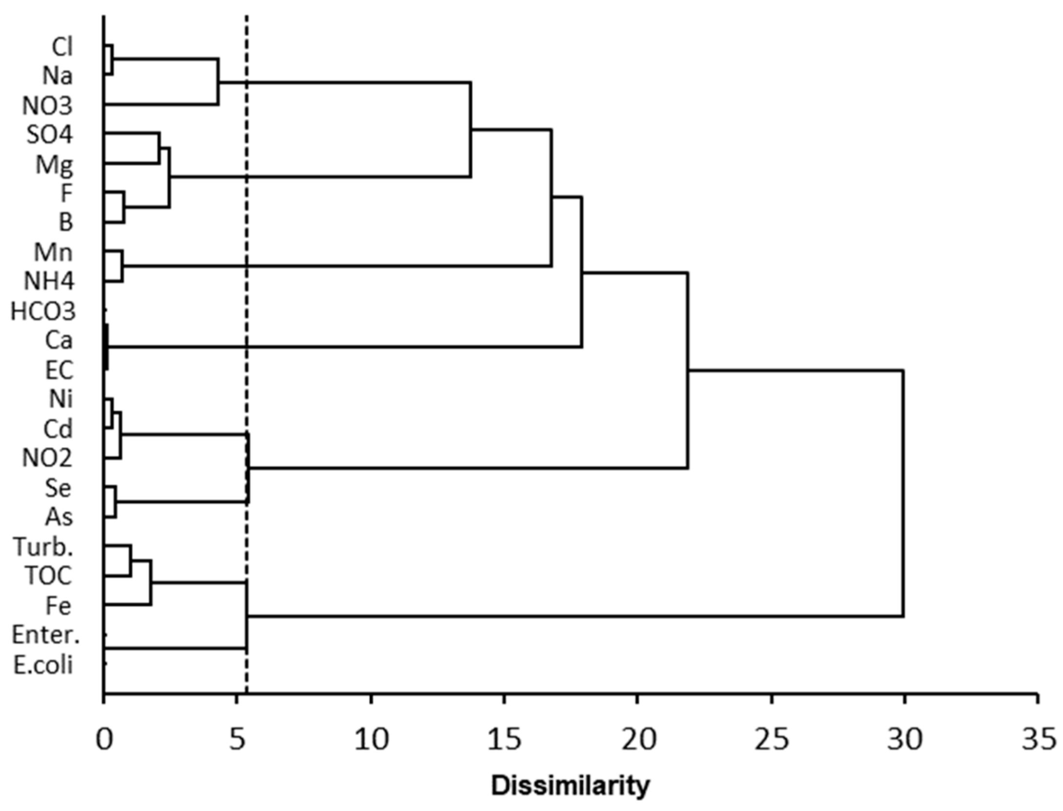
3.2. Parameter Clustering

The classification of parameters based on their correlation allowed us to distinguish six groups (Figure 6). The first group consisted of E.coli and Enter. parameters, which were strongly correlated with each other and associated with turbidity, TOC, and Fe. This set of five parameters, characteristic of surface waters, was completely distinct from the others. The metalloids arsenic and selenium, along with the metals cadmium and nickel, formed another group of parameters that also stood out. Calcium, bicarbonates, and electrical conductivity made up a third well-defined group. A fourth group included manganese and ammonium, which are characteristic of more reducing environments. Finally, the last two groups, which were more heterogeneous, consisted of the remaining seven water quality parameters: on one hand, magnesium, sulfate, fluoride, and boron, and on the other hand, sodium, chloride, and nitrate.

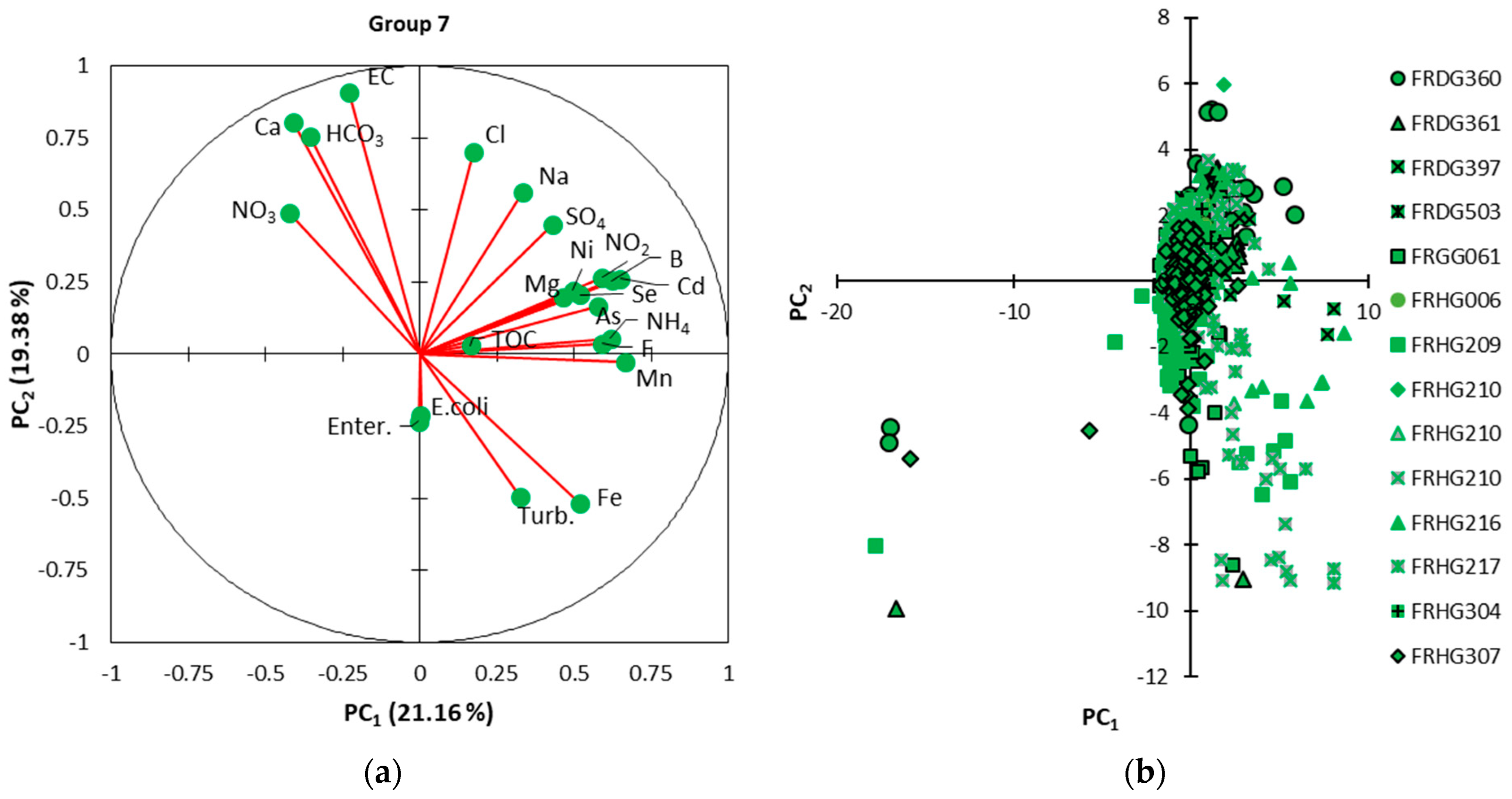
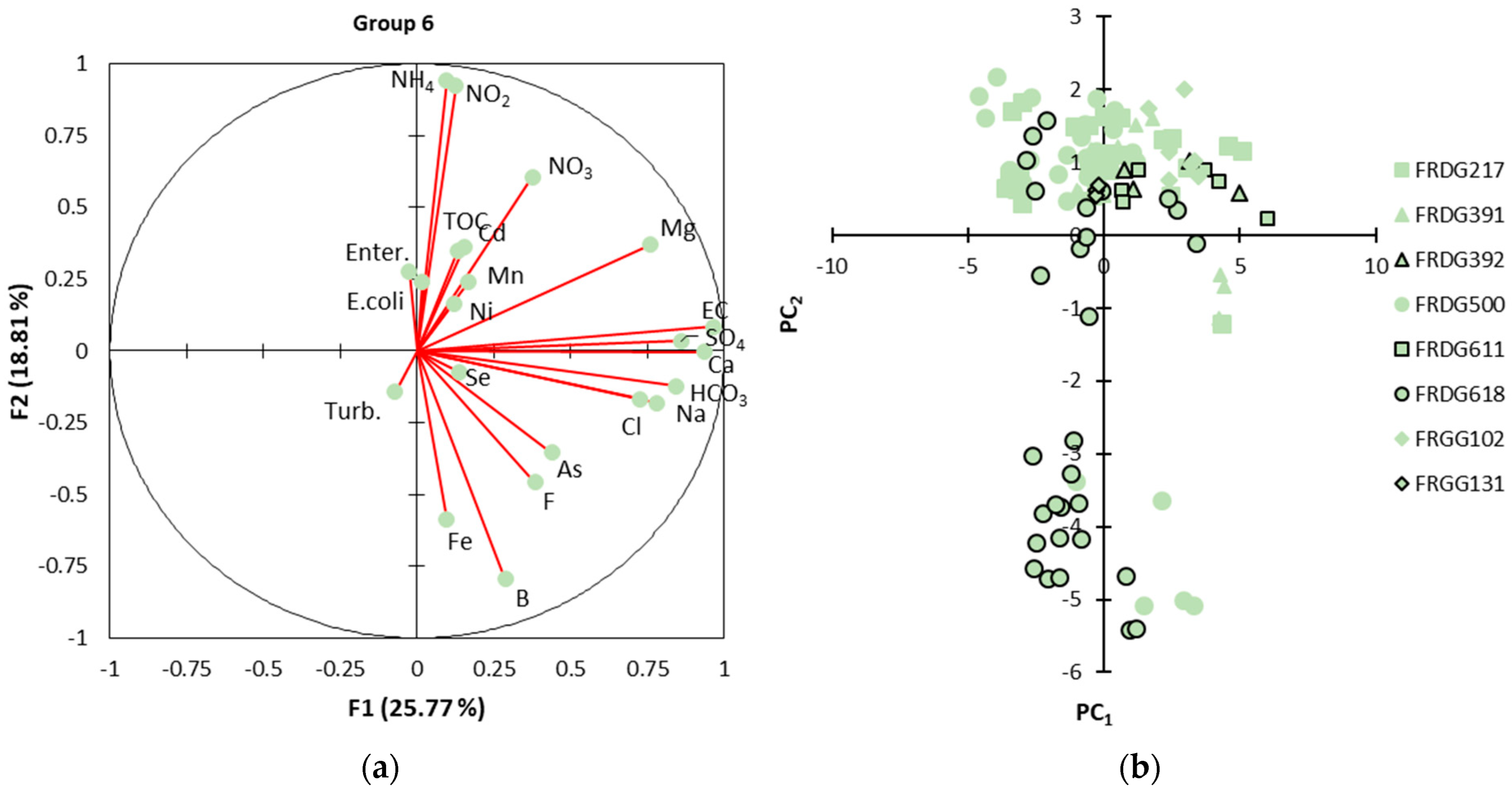
3.3. Characteristics of the Groups

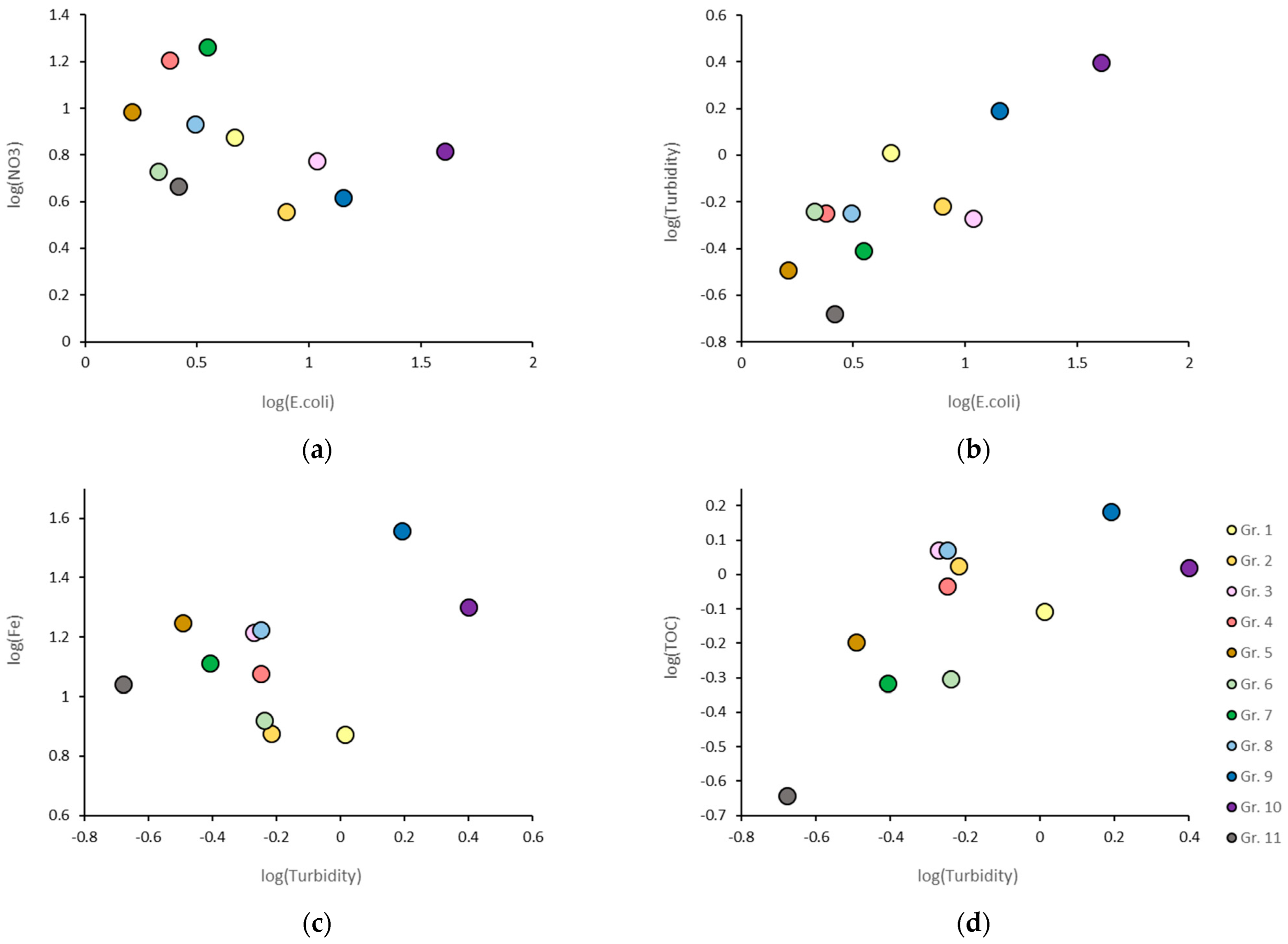
3.3.1. Fecal Contamination and Nitrogen Pollution

Figure 6 suggests that bacteriological parameters and nitrates, which were positioned far apart on the dendrogram, convey very different information. Furthermore, according to the Regional Health Agencies, fecal contamination represents the main non-compliance issue for groundwater intended for consumption, whereas NO₃⁻ is one of the major concerns in terms of the frequency of high values. Therefore, as a first step, these two parameters should be compared (Figure 7a). The GWB from Groups 3, 9, and especially 10 were characterized by significant fecal contamination but moderate nitrogen pollution. Group 2 was similar to these three groups, showing low nitrogen pollution but moderate fecal contamination.

At the other extreme, Groups 4 and 7 exhibited the highest nitrogen pollution levels in the region, while fecal contamination remained lower. Group 6 (and, to a lesser extent, Group 11, which consisted of a single GWB) displayed good bacteriological characteristics and low nitrate concentrations.

3.3.2. Fecal Contamination and Associated Parameters

Groups 9 and 10, which were the most affected by fecal contamination, also corresponded to groundwater with high turbidity (Figure 7b), confirming the role of particles responsible for turbidity in bacterial transport. A strong correlation appeared for Groups 1, 4, 6, 8, 9, and 10. Groups 2 and 3, where moderate contamination was observed despite relatively low turbidity, and Groups 11, 5, and 7, where contamination was low, deviate from this correlation. The comparison of turbidity with Fe (Figure 7c) generally showed a positive correlation, suggesting that ferric colloids contributed to the particle load. This correlation was evident for Groups 3, 5, 7, 8, 9, and 11, while Groups 1, 2, and 6 deviated from it. The contribution of iron to turbidity was less significant in these groups compared to others, suggesting that turbidity is influenced by other components. GWB Groups 4 and 10 presented an intermediate situation, possibly reflecting a different nature of turbidity. TOC increased with turbidity, suggesting that organic carbon also contributes to turbidity (Figure 7d). However, this positive correlation was distributed into two distinct sets. In Groups 2, 3, 4, 5, and 9, the TOC contribution to turbidity was higher, implying that organic matter plays a greater role in turbidity composition. Notably, Groups 9 and 10, which are the most affected by fecal contamination, exhibited high turbidity levels and elevated organic carbon concentrations.

3.3.3. Turbidity and Water Minerality

Overall, turbidity decreased with the mineral content of the water, which could be explained by the flocculation effect of mineralized water. The flocculation of particles reduces their detachment, thereby lowering turbidity. This particularly explained the high turbidity and, consequently, the elevated bacterial load in the groundwater of Group 10. Two GWB groups with the most diluted water in the region, namely Groups 6 and 9, stood out from this general trend.

3.3.4. Parameters Sensitive to Redox Conditions

Three of the parameters included in the dataset are sensitive to redox conditions: manganese, iron, and nitrite. Nine out of the eleven groups exhibited a correlation between Mn and NO₂ (Figure 8b). Groups 8, 9, and 10 appeared to be the richest in nitrites and manganese, suggesting rather reducing conditions. Conversely, Groups 3 and 5 seemed to correspond to the most oxidizing conditions. It is worth noting that Groups 2 and 4 clearly deviated from this correlation between the two parameters.

3.4. Water Quality Homogeneity Within Groups

While the groups differ in terms of average characteristics, it is important to examine the internal variability of each group. To illustrate this, three groups were selected: Group 7, representing GWB rich in nitrates with low fecal contamination; Group 9, representing GWB vulnerable to fecal contamination; and Group 6, representing GWB with minimally contaminated water in terms of both fecal and nitrogen pollution. The results of the ANOVA concerning these three groups are presented in

Table 2. Results of the ANOVA showing inter-sampling point and inter-GWB explained variance for Groups 7, 6, and 9.

	Group 7		Group 9		Group 6
Parameter	GWB	Catch. Point	GWB	Catch. Point	GWB	Catch. Point
EC	0.08	0.86	0.02	0.97	0.25	0.98
E.coli	0.05	0.60	0.08	0.88	0.05	0.78
Enter	0.05	0.57	0.10	0.91	0.04	0.62
NH4	0.04	0.75	0.03	0.53	0.34	0.85
As	0.05	0.77	0.00	0.76	0.01	0.76
Na	0.44	0.86	0.02	0.90	0.46	0.97
Ca	0.03	0.84	0.03	0.98	0.20	0.97
Mg	0.42	0.91	0.07	0.96	0.28	0.99
Cl	0.31	0.83	0.04	0.90	0.31	0.89
SO4	0.31	0.89	0.09	0.95	0.33	0.97
HCO3	0.04	0.83	0.02	0.96	0.11	0.98
NO3	0.10	0.86	0.11	0.64	0.49	0.96
Fe	0.09	0.71	0.10	0.85	0.08	0.58
Mn	0.15	0.71	0.15	0.79	0.24	0.71
B	0.23	0.79	0.01	0.69	0.13	0.71
F	0.28	0.79	0.09	0.91	0.12	0.95
NO2	0.02	0.93	0.05	0.70	0.36	0.82
TOC	0.12	0.66	0.15	0.95	0.19	0.48
Turb.	0.09	0.70	0.17	0.86	0.12	0.71
Se	0.02	0.86	0.05	0.93	0.13	0.54
Cd	0.02	1.00	0.00	1.00	0.21	0.60
Ni	0.02	0.77	0.03	1.00	0.15	0.56

. It shows that the inter-catchment point variance is high, accounting for nearly all of the total variance for major ions (between 83 and 98%) and bacteriological parameters (between 57 and 91%) but is also high for minor and trace elements (between 54 and 100%). The proportion of temporal variance, corresponding to the complement to 1 of the inter-catchment points explained variance, is low for major ions (around 1%) and moderate for bacteriological parameters (9 to 40%) and trace elements (6 to 45%). On the other hand, the explained variance at the inter-GWB scale is moderate (1 to 17%), which indicates a homogeneous grouping of GWBs.

The PCAs conducted for these three groups (7, 9, and 6) (Figure 9, Figure 10 and Figure 11) allow visualization of the dispersion of parameters and observations in the first factorial plane, which accounts for 40.5%, 51.3%, and 44.6% of the variance, respectively. The results showed good homogeneity within the groups, as the representative points of each GWB overlapped relatively well with those of other GWBs within the same group (Figure 9b, Figure 10b, and Figure 11b). It was also observed that the first factorial planes of each group were very different from one another. For Group 7, representing nitrogen contamination, fecal contamination did not play a significant role in the first factorial plane, where the first axis contrasted carbonate-calcium and nitrate-rich mineralized waters with waters rich in ammonium, nitrites, manganese, and iron.

For Group 9, affected by high fecal contamination, the first factorial axis contrasted mineralized waters loaded with E. coli and Enterococci with nitrate-rich waters, while the second factorial axis contrasted carbonate-calcium and nitrate-rich waters with feces-contaminated waters characterized by turbidity, TOC, and the presence of iron and manganese. Finally, for Group 6, representing waters with low fecal and nitrate contamination, the first factorial axis reflected water mineralization, while the second axis represented nitrogen pollution.

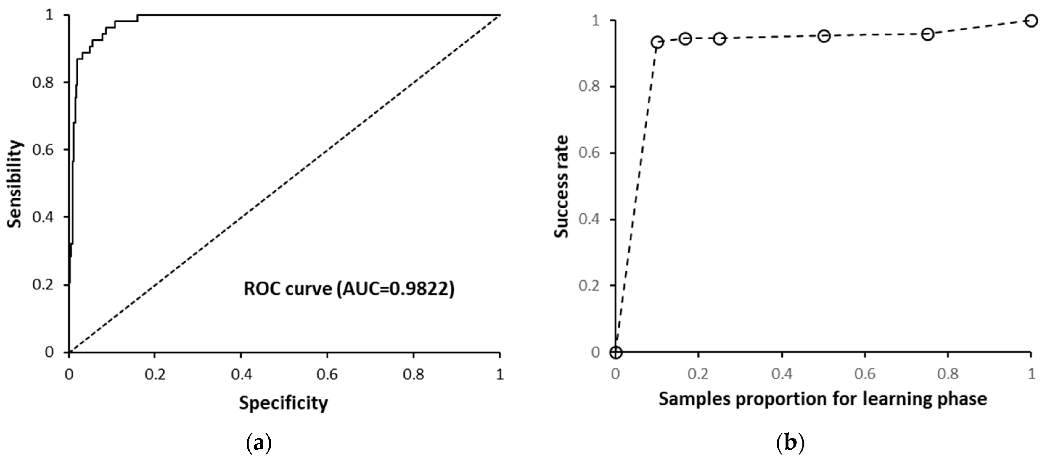
3.5. Discrimination of Groups 9 and 10

As mentioned earlier, fecal contamination is by far the most frequent cause of non-compliance in water intended for human consumption in France. Within the region, Groups 9 and 10 were the most affected by fecal contamination (Figure 7a,b, and Table 1). A review of the GWB clustering showed that these two groups shared very similar characteristics across all parameters. In the case of a classification into 10 groups—i.e., with the phenom line set at a slightly higher dissimilarity value—these two GWB groups would be merged (Figure 4). Although the difference between them is small, it is still necessary to characterize it. Group 9 consisted of 340 water samples distributed across 3 GWBs, while Group 10 consisted of 60 water samples, also distributed across 3 other GWBs. The confusion matrix from the linear discriminant analysis is presented in

Table 3. Confusion matrix resulting from the linear discriminant analysis.

from\to	9	10	Total	% Correct
9	334	13	347	96.25%
10	6	47	53	88.68%
Total	340	60	400	95.25%

and shows that 95% of the samples are correctly classified. Among the 19 misclassified samples, 14 belong to FRGG046, which has an uncertain origin in the database. Indeed, this water source is listed as the “Bourbince water intake” in the commune of Paray-le-Monial, yet the term “water intake” is generally associated with surface water sources. It is possible that this source was misclassified when entered into the database. Aside from this sampling point—where only part of the samples was misclassified by the LDA—the overall classification score remained very high.

The standardized coefficients of the canonical discriminant function (F1,

Table 4. Standardized coefficients of the canonical discriminant function.

Param.	F1	Param.	F1	Param.	F1	Param.	F1
EC	1.364	Na	0.211	HCO3	−0.597	F	−0.382
E.coli	0.754	Ca	0.527	NO3	−0.382	NO2	0.023
Enter.	−0.351	Mg	−0.254	Fe	0.216	TOC	−0.842
NH4	−0.018	Cl	−0.030	Mn	−0.119	Turb.	0.472
As	−0.356	SO4	−0.178	B	0.247

) indicated that the differentiation between these two groups was primarily based on the minerality of the waters (low for Group 9 and higher for Group 10), fecal contamination by E. coli, calcium content, and turbidity. These parameters contrasted with TOC, nitrate, Enterococcus, As, and HCO₃. On the other hand, the other parameters (NH₄, Na, Mg, Cl, SO₄, Mn, NO₂, etc.) played only a minor role in the differentiation.

The ROC curve (Figure 12a) displayed a trajectory well above the diagonal, with an area under the curve (AUC) of 0.9822, confirming the strong discriminatory power. The Naïve Bayesian classifier performed comparably to the linear discriminant analysis, achieving 93.6% correct classification with just 10% of samples used for training (Figure 12b). When increasing the training set to 50%, accuracy improved slightly to 95.5%.

4. Discussion

The integration of the two databases, Size-Eaux and the French Groundwater Bodies Reference System, led to the classification of 11 distinct groups. The specific study of these groups helps in understanding a wide range of ongoing processes, ultimately contributing to the optimized management of water resources.

4.1. Consistent Discrimination and Grouping of GWBs

The results of the ANOVA performed on the three groups (7, 9, and 6) highlight homogeneity among GWBs (Groundwater Bodies) within the same group. Furthermore, on the first factorial planes (Figure 9, Figure 10 and Figure 11), the clusters representing different GWBs (Groundwater Bodies) within the same group overlap, whereas the factorial planes of different groups are defined by distinct parameter associations. These results demonstrate a strong differentiation between GWB groups, confirming a discrimination that strongly incorporates spatial variability—particularly for the two main contamination types: fecal and nitrogen-based. They suggest:

• The relevance of the method used, which groups GWBs not only based on similar overall parameter characteristics (i.e., proximity in features) but also on correlations between these parameters (i.e., similar underlying mechanisms). At the same time, GWB groups with markedly different factorial planes reflect distinct mechanisms and variability sources from one group to another.
• Stability in chemical and microbiological characteristics within groups, with variability mainly linked to temporal quality fluctuations at the catchment scale [31].

The method for determining GWB groups thus proves effective. Despite the region’s size and diversity (lithological, altitudinal, etc.), it is not an obstacle, as ultimately only eleven distinct but homogeneous units can be more easily managed by monitoring agencies.

4.2. Contamination in Line with Lithology and Land Use

Groups 9 and 10, located in the south-central, western, and southwestern parts of the region, correspond to a crystalline mountain zone (metamorphic and plutonic formations) and a sector with Mesozoic sedimentary terrain (Upper Jurassic), respectively. These areas concentrate most of the region’s intensive beef cattle farming (http://sg-proxy02.maaf.ate.info/en-region/bourgogne-franche-comte/, accessed in 6 January 2025). These two groups stand out due to high levels of biological contaminants, which can be explained by multiple factors. First, the proximity to livestock farming areas, where slurry and manure spreading practices facilitate bacterial infiltration into aquifers, plays a crucial role. The high pollution pressure is a determining factor. Additionally, the frequent obsolescence of individual sanitation systems in rural areas increases the risk of untreated wastewater infiltration into groundwater.

Beyond land use, natural environmental characteristics contribute to contamination, particularly in Group 9. GWBs in this group develop within weathered granites, schists, and sandstones, with sandy soils that promote rapid infiltration of contaminated surface water, especially during heavy rainfall at the end of summer [26,31]. Low mineralization and the absence of flocculating cations contribute to high turbidity, whether from clay particles, organic matter, or colloids. In this context, both iron and manganese reflect conditions of surface particulate transport. Additionally, streams crossing Group 9 interact with groundwater, facilitating the transfer of bacterial pollutants from urbanized and agricultural areas.

In the case of Group 10, the soils consist of thin skeletal formations developed on limestone, where percolation is rapid. The waters in this group are more concentrated, but turbidity is high, enhancing bacterial transport. The strong contribution of Total Organic Carbon (TOC) to turbidity in Group 10 explains the reducing nature of the water, with high NO₂ and Mn parameters, as oxygen is consumed by bacteria oxidizing organic carbon.

Groups 4 and 7 correspond to aquifers in sedimentary formations with limestone and chalk lithology. These lands are mainly used for cereal and large-scale farming, with secondary use for vineyards (notably Chablis and Bourgogne-Côte d’Auxerre). Fertilization is widespread in these areas, making nitrogen pollution the highest observed in the Bourgogne-Franche-Comté (BFC) region. However, due to low livestock pressure, fecal contamination remains infrequent.

In the Jura sectors (Groups 2 and 3), bacterial contamination pressure is high due to concentrated dairy farming activity. However, the presence of marl layers (within a marl-limestone context) limits infiltration and the transfer of surface water into groundwater.

4.3. Existence of Regional Structures Beyond Local Specificities

The identification of homogeneous groups of groundwater bodies in Bourgogne-Franche-Comté focused on the two major types of contamination—fecal and nitrogen—each linked to distinct processes. This approach helps transcend local specificities to define appropriate protection strategies on a regional scale.

For groups affected by fecal contamination, previous studies have highlighted the critical role of groundwater vulnerability to surface water infiltration, which carries pathogens [24,46]. Specifically, the separation of temporal and spatial variance within this dataset for Bourgogne-Franche-Comté demonstrated that contamination is episodic and linked to rainfall events [31]. Targeted solutions should focus on protecting water intakes from surface water inflows, which act as contamination vectors, with intensified monitoring following heavy rainfall. Special attention should be given to manure storage on plots before spreading, as such deposits often remain in place for weeks and may contribute to contaminant plumes reaching groundwater.

Conversely, for groups affected by nitrogen contamination, pollution is chronic, agricultural in origin, and affects groundwater independently of rainfall events, requiring proactive agronomic management. Monitoring should not be event-driven but conducted long-term. Prevention should focus on improved fertilization management, including:

• The type of fertilizer (ammoniacal/nitrate forms).
• The quantity (aligned with crop needs).
• The application schedule (adjusted to the crop growth cycle throughout the agricultural season).

The establishment of GWB groups allows for a refined understanding of ongoing landscape processes. Future research could involve developing digital maps based on the factorial axis coordinates from the specific analyses of each group. For instance, in Group 9, a map of the coordinates on PC2 could indicate the conditions that make water intakes vulnerable to bacterial contamination (lithology, fracture zones, slope, etc.). For Group 7, a digital map based on PC1 coordinates could highlight the structure of the denitrification process—its presence or absence—on a broader scale beyond individual water catchments. This information could help prioritize actions. Thus, the classification of homogeneous GWB groups should be viewed as a tool to extrapolate findings beyond individual cases, facilitating an integrated landscape management approach through optimized protective measures.

4.4. Applicability and Limitations of the Method

The initial division into 70 GWBs (Groundwater Bodies) established by the French Geological Survey across the entire Bourgogne-Franche-Comté (BFC) region proves excessive for targeted and effective water quality monitoring by the Regional Health Agency. Conversely, the 11 GWB groups, which form homogeneous units in terms of physico-chemical and bacteriological characteristics, as well as the underlying mechanisms driving these parameters, allow for the development of a relevant and focused monitoring strategy.

One potential limitation to the applicability of the method could be the presence of outliers, errors, or referencing issues within the Sise-Eaux database. The logarithmic transformation applied prior to any processing has been tested repeatedly and quantified in the Occitanie and Provence-Alpes-Côte d’Azur regions, reducing the influence of outlier values that could otherwise obscure the core information, i.e., that carried by non-extreme values [19,32]. Furthermore, GWBs are exploitable water bodies, meaning they have a certain volume and, consequently, a certain inertia. As there are multiple analyses per sampling point and multiple sampling points per GWB, this ensures a significant averaging effect and a certain level of representativeness in the face of potentially erroneous values or misclassified results in the database.

The approach applied here has also been tested in other French regions, covering areas ranging from 8000 to 80,000 km², with highly varied contrasts in lithology, elevation, climate, and land use. A similar study conducted in Occitanie [18], a region larger than Bourgogne-Franche-Comté (73,000 vs. 48,000 km², respectively), highlighted the need to divide the territory into two major sectors. This division was not driven by the region’s size but by a stark climatic contrast between its Atlantic-facing and Mediterranean-facing slopes, accompanied by very different agricultural practices. Thus, splitting the region into two subregions helped minimize information loss during the grouping of GWBs. This outcome, which resulted in distinguishing the Adour-Garonne and Rhône-Méditerranée basins, also aligned with the requirements of the Water Framework Directive [47,48], which calls for a division by major river basins [27,30,49].

Unlike in Occitanie, in BFC—spanning three major basins (Seine, Loire, and Rhône)—the absence of strong contrast between these sectors does not affect the quality of the grouping, as numerous cases exist where GWBs from different basins are grouped together (Figure 4). This had already been observed in the Auvergne-Rhône-Alpes region [16], also straddling three major basins (Loire, Rhône, and Garonne), even though in that administrative region, we observed that the groups were generally distributed within one or the other of these basins, thus somewhat validating the Water Framework Directive approach that recommends an inventory of groundwater bodies based on major European river basins.

This method is therefore flexible and applicable to various geological and hydrogeological contexts, provided, of course, that a statistically significant number of samples per observation point and per GWB are available. Interpretation is naturally guided case by case by local specificities: geological formations, land use, and potential contamination sources. From this perspective—and unfortunately, this is not the case for most European countries—France benefits from a substantial database (Sise-Eaux) with over 32,000 groundwater sampling points, regularly updated for more than 30 years and including numerous physico-chemical and bacteriological parameters (over 100), with the list expanding as analytical capabilities advance [50,51].

Regarding GWB delineation, however, many countries have responded to the Water Framework Directive initiative [52,53,54,55,56,57,58,59,60,61,62], and the delineation of groundwater bodies does not appear to be a limiting factor in extending this method to other European countries.

5. Conclusions

This study aimed to classify the groundwater bodies of the Bourgogne-Franche-Comté region (France) into homogeneous groups, both in terms of water characteristics and the mechanisms responsible for their diversity. To achieve this, it relied on the cross-analysis of the Sise-Eaux database and the French Groundwater Body Reference Framework, with the ultimate goal of optimizing resource monitoring and surveillance by the responsible agencies (Regional Health Agencies). Based on 989 sampling points distributed across 70 GWBs, the results identified 11 groups, revealing strong differentiation between them, as well as significant internal homogeneity. The marked spatial structuring of geological formations facilitated a relevant grouping of GWB, with each group displaying well-defined specificities, particularly regarding nitrate and fecal contamination. The grouping method proved effective for groundwater management at the regional scale, even in a vast (48,000 km²) and heterogeneous region such as Bourgogne-Franche-Comté, spanning three major watershed basins. This approach provides a valuable tool for groundwater monitoring and protection, enabling the implementation of a targeted surveillance strategy tailored to the specificities of each of the 11 groups while considering local characteristics and the processes influencing water quality.

References

1. Bhunia, G.S.; Shit, P.K.; Brahma, S. Chapter 19—Groundwater Conservation and Management: Recent Trends and Future Prospects. In Case Studies in Geospatial Applications to Groundwater Resources; Shit, P.K., Bhunia, G.S., Adhikary, P.P., Eds.; Elsevier: Amsterdam, The Netherlands, 2023; pp. 371–385. ISBN 978-0-323-99963-2. [Google Scholar]
2. Kemper, K.E. Groundwater—From Development to Management. Hydrogeol. J. 2004, 12, 3–5. [Google Scholar] [CrossRef]
3. Falkenmark, M.; Folke, C.; Foster, S.S.D.; Chilton, P.J. Groundwater: The Processes and Global Significance of Aquifer Degradation. Philos. Trans. R Soc. Lond. B 2003, 358, 1957–1972. [Google Scholar] [CrossRef]
4. Motlagh, A.M.; Yang, Z.; Saba, H. Groundwater Quality. Water Environ. Res. 2020, 92, 1649–1658. [Google Scholar] [CrossRef]
5. van der Gun, J. Chapter 24—Groundwater Resources Sustainability. In Global Groundwater; Mukherjee, A., Scanlon, B.R., Aureli, A., Langan, S., Guo, H., McKenzie, A.A., Eds.; Elsevier: Amsterdam, The Netherlands, 2021; pp. 331–345. ISBN 978-0-12-818172-0. [Google Scholar]
6. Yuan, H.; Yang, S.; Wang, B. Hydrochemistry Characteristics of Groundwater with the Influence of Spatial Variability and Water Flow in Hetao Irrigation District, China. Environ. Sci. Pollut. Res. 2022, 29, 71150–71164. [Google Scholar] [CrossRef] [PubMed]
7. Gao, Y.; Chen, J.; Qian, H.; Wang, H.; Ren, W.; Qu, W. Hydrogeochemical Characteristics and Processes of Groundwater in an over 2260 Year Irrigation District: A Comparison between Irrigated and Nonirrigated Areas. J. Hydrol. 2022, 606, 127437. [Google Scholar] [CrossRef]
8. Sophocleous, M. Review: Groundwater Management Practices, Challenges, and Innovations in the High Plains Aquifer, USA—Lessons and Recommended Actions. Hydrogeol. J. 2010, 18, 559–575. [Google Scholar] [CrossRef]
9. Ielpo, P.; Cassano, D.; Felice Uricchio, V.; Lopez, A.; Pappagallo, G.; Trizio, L.; de Gennaro, G. Identification of Pollution Sources and Classification of Apulia Region Groundwaters by Multivariate Statistical Methods and Neural Networks. Trans. ASABE 2013, 56, 1377–1386. [Google Scholar] [CrossRef]
10. Doctor, D.H.; Alexander, E.C.; Petrič, M.; Kogovšek, J.; Urbanc, J.; Lojen, S.; Stichler, W. Quantification of Karst Aquifer Discharge Components during Storm Events through End-Member Mixing Analysis Using Natural Chemistry and Stable Isotopes as Tracers. Hydrogeol. J. 2006, 14, 1171–1191. [Google Scholar] [CrossRef]
11. Woldt, W.; Bogardi, I. Ground Water Monitoring Network Design Using Multiple Criteria Decision Making and Geostatistics. J. Am. Water Resour. Assoc. 1992, 28, 45–62. [Google Scholar] [CrossRef]
12. Bárdossy, A. Copula-Based Geostatistical Models for Groundwater Quality Parameters. Water Resour. Res. 2006, 42, W11416. [Google Scholar] [CrossRef]
13. Sheikhy Narany, T.; Ramli, M.F.; Aris, A.Z.; Sulaiman, W.N.A.; Fakharian, K. Spatiotemporal Variation of Groundwater Quality Using Integrated Multivariate Statistical and Geostatistical Approaches in Amol-Babol Plain, Iran. Environ. Monit. Assess. 2014, 186, 5797–5815. [Google Scholar] [CrossRef] [PubMed]
14. Masoud, A.A. Groundwater Quality Assessment of the Shallow Aquifers West of the Nile Delta (Egypt) Using Multivariate Statistical and Geostatistical Techniques. J. Afr. Earth Sci. 2014, 95, 123–137. [Google Scholar] [CrossRef]
15. Machiwal, D.; Jha, M.K. Identifying Sources of Groundwater Contamination in a Hard-Rock Aquifer System Using Multivariate Statistical Analyses and GIS-Based Geostatistical Modeling Techniques. J. Hydrol. Reg. Stud. 2015, 4, 80–110. [Google Scholar] [CrossRef]
16. Ayach, M.; Lazar, H.; Lamat, C.; Bousouis, A.; Touzani, M.; El Jarjini, Y.; Kacimi, I.; Valles, V.; Barbiero, L.; Morarech, M. Groundwaters in the Auvergne-Rhône-Alpes Region, France: Grouping Homogeneous Groundwater Bodies for Optimized Monitoring and Protection. Water 2024, 16, 869. [Google Scholar] [CrossRef]
17. Lazar, H.; Ayach, M.; Barry, A.A.; Mohsine, I.; Touiouine, A.; Huneau, F.; Mori, C.; Garel, E.; Kacimi, I.; Valles, V.; et al. Groundwater Bodies in Corsica: A Critical Approach to GWBs Subdivision Based on Multivariate Water Quality Criteria. Hydrology 2023, 10, 213. [Google Scholar] [CrossRef]
18. Jabrane, M.; Touiouine, A.; Valles, V.; Bouabdli, A.; Chakiri, S.; Mohsine, I.; El Jarjini, Y.; Morarech, M.; Duran, Y.; Barbiero, L. Search for a Relevant Scale to Optimize the Quality Monitoring of Groundwater Bodies in the Occitanie Region (France). Hydrology 2023, 10, 89. [Google Scholar] [CrossRef]
19. Mohsine, I.; Kacimi, I.; Valles, V.; Leblanc, M.; El Mahrad, B.; Dassonville, F.; Kassou, N.; Bouramtane, T.; Abraham, S.; Touiouine, A.; et al. Differentiation of Multi-Parametric Groups of Groundwater Bodies through Discriminant Analysis and Machine Learning. Hydrology 2023, 10, 230. [Google Scholar] [CrossRef]
20. Tiouiouine, A.; Jabrane, M.; Kacimi, I.; Morarech, M.; Bouramtane, T.; Bahaj, T.; Yameogo, S.; Rezende-Filho, A.T.; Dassonville, F.; Moulin, M.; et al. Determining the Relevant Scale to Analyze the Quality of Regional Groundwater Resources While Combining Groundwater Bodies, Physicochemical and Biological Databases in Southeastern France. Water 2020, 12, 3476. [Google Scholar] [CrossRef]
21. Chery, L.; Laurent, A.; Vincent, B.; Tracol, R. Echanges SISE-Eaux/ADES: Identification Des Protocoles Compatibles Avec Les Scénarios d’échange SANDRE; Office National de l’Eau et des Milieux Aquatiques: Bron, France, 2011. [Google Scholar]
22. Gran-Aymeric, L. Un Portail National Sur La Qualite Des Eaux Destinees a La Consommation Humaine. Tech. Sci. Méthodes 2010, 12, 45–48. [Google Scholar] [CrossRef]
23. John, D.E.; Rose, J.B. Review of Factors Affecting Microbial Survival in Groundwater. Environ. Sci. Technol. 2005, 39, 7345–7356. [Google Scholar] [CrossRef]
24. Pachepsky, Y.A.; Shelton, D.R. Escherichia Coli and Fecal Coliforms in Freshwater and Estuarine Sediments. Crit. Rev. Environ. Sci. Technol. 2011, 41, 1067–1110. [Google Scholar] [CrossRef]
25. Pandey, P.K.; Kass, P.H.; Soupir, M.L.; Biswas, S.; Singh, V.P. Contamination of Water Resources by Pathogenic Bacteria. AMB Express 2014, 4, 51. [Google Scholar] [CrossRef] [PubMed]
26. Bousouis, A.; Bouabdli, A.; Ayach, M.; Ravung, L.; Valles, V.; Barbiero, L. The Multi-Parameter Mapping of Groundwater Quality in the Bourgogne-Franche-Comté Region (France) for Spatially Based Monitoring Management. Sustainability 2024, 16, 8503. [Google Scholar] [CrossRef]
27. European Commission. Directive 2006/118/EC of the European Parliament and of the Council of 12 December 2006 on the Protection of Groundwater against Pollution and Deterioration. Off. J. Eur. Union 2006, 372, 19–31. [Google Scholar]
28. Wendland, F.; Blum, A.; Coetsiers, M.; Gorova, R.; Griffioen, J.; Grima, J.; Hinsby, K.; Kunkel, R.; Marandi, A.; Melo, T.; et al. European Aquifer Typology: A Practical Framework for an Overview of Major Groundwater Composition at European Scale. Environ. Geol. 2008, 55, 77–85. [Google Scholar] [CrossRef]
29. European Commission. Guidance Document No. 22. Guidance on Implementing the Geographical Information System (GIS) Elements of the EU Water Policy. Tools and Services for Reporting Under RBMP Within WISE. Guidance on Reporting of Spatial Data for the WFD (RBMP); Atkins: London, UK, 2009. [Google Scholar]
30. Duscher, K. Compilation of a Groundwater Body GIS Reference Layer. In Proceedings of the Presentation at the WISE GIS Workshop, Copenhagen, Denmark, 16–17 November 2010. [Google Scholar]
31. Bousouis, A.; Bouabdli, A.; Ayach, M.; Lazar, H.; Ravung, L.; Valles, V.; Barbiero, L. Discrimination of Spatial and Temporal Variabilities in the Analysis of Groundwater Databases: Application to the Bourgogne-Franche-Comté Region, France. Water 2025, 17, 384. [Google Scholar] [CrossRef]
32. Jabrane, M.; Touiouine, A.; Bouabdli, A.; Chakiri, S.; Mohsine, I.; Valles, V.; Barbiero, L. Data Conditioning Modes for the Study of Groundwater Resource Quality Using a Large Physico-Chemical and Bacteriological Database, Occitanie Region, France. Water 2023, 15, 84. [Google Scholar] [CrossRef]
33. Mohsine, I.; Kacimi, I.; Abraham, S.; Valles, V.; Barbiero, L.; Dassonville, F.; Bahaj, T.; Kassou, N.; Touiouine, A.; Jabrane, M.; et al. Exploring Multiscale Variability in Groundwater Quality: A Comparative Analysis of Spatial and Temporal Patterns via Clustering. Water 2023, 15, 1603. [Google Scholar] [CrossRef]
34. Ayach, M.; Lazar, H.; Bousouis, A.; Touiouine, A.; Kacimi, I.; Valles, V.; Barbiero, L. Multi-Parameter Analysis of Groundwater Resources Quality in the Auvergne-Rhône-Alpes Region (France) Using a Large Database. Resources 2023, 12, 143. [Google Scholar] [CrossRef]
35. Lazar, H.; Ayach, M.; Bousouis, A.; Huneau, F.; Mori, C.; Garel, E.; Kacimi, I.; Valles, V.; Barbiero, L. Multivariate and Spatial Study and Monitoring Strategies of Groundwater Quality for Human Consumption in Corsica. Hydrology 2024, 11, 197. [Google Scholar] [CrossRef]
36. Helena, B.; Pardo, R.; Vega, M.; Barrado, E.; Fernandez, J.M.; Fernandez, L. Temporal Evolution of Groundwater Composition in an Alluvial Aquifer (Pisuerga River, Spain) by Principal Component Analysis. Water Res. 2000, 34, 807–816. [Google Scholar] [CrossRef]
37. Bouguettaya, A.; Yu, Q.; Liu, X.; Zhou, X.; Song, A. Efficient Agglomerative Hierarchical Clustering. Expert Syst. Appl. 2015, 42, 2785–2797. [Google Scholar] [CrossRef]
38. Suk, H.; Lee, K.-K. Characterization of a Ground Water Hydrochemical System Through Multivariate Analysis: Clustering into Ground Water Zones. Groundwater 1999, 37, 358–366. [Google Scholar] [CrossRef]
39. Madhulatha, T.S. An Overview on Clustering Methods. IOSR J. Eng. 2012, 2, 719–725. [Google Scholar] [CrossRef]
40. Huberty, C.J. Discriminant Analysis. Rev. Educ. Res. 1975, 45, 543–598. [Google Scholar] [CrossRef]
41. Amiri, V.; Nakagawa, K. Using a Linear Discriminant Analysis (LDA)-Based Nomenclature System and Self-Organizing Maps (SOM) for Spatiotemporal Assessment of Groundwater Quality in a Coastal Aquifer. J. Hydrol. 2021, 603, 127082. [Google Scholar] [CrossRef]
42. Bradley, A.P. The Use of the Area under the ROC Curve in the Evaluation of Machine Learning Algorithms. Pattern Recognit. 1997, 30, 1145–1159. [Google Scholar] [CrossRef]
43. Rish, I. An Empirical Study of the Naive Bayes Classifier. In Proceedings of the IJCAI 2001 workshop on empirical methods in artificial intelligence, Seattle, WA, USA, 4–6 August 2001; pp. 41–46. [Google Scholar]
44. Achen, C.H. What Does “Explained Variance” Explain?: Reply. Political Anal. 1990, 2, 173–184. [Google Scholar] [CrossRef]
45. Miles, J. R Squared, Adjusted R Squared. In Wiley StatsRef: Statistics Reference Online; Wiley: Hoboken, NJ, USA, 2014; ISBN 9781118445112. [Google Scholar]
46. Abbas, A.; Baek, S.; Silvera, N.; Soulileuth, B.; Pachepsky, Y.; Ribolzi, O.; Boithias, L.; Cho, K.H. In-Stream Escherichia coli Modeling Using High-Temporal-Resolution Data with Deep Learning and Process-Based Models. Hydrol. Earth Syst. Sci. 2021, 25, 6185–6202. [Google Scholar] [CrossRef]
47. Chave, P. The EU Water Framework Directive—An Introduction; IWA Publishing: London, UK, 2007; ISBN 9781780402239. [Google Scholar]
48. Kallis, G.; Butler, D. The EU Water Framework Directive: Measures and Implications. Water Policy 2001, 3, 125–142. [Google Scholar] [CrossRef]
49. Wendland, F.; Berthold, G.; Blum, A.; Elsass, P.; Fritsche, J.-G.; Kunkel, R.; Wolter, R. Derivation of Natural Background Levels and Threshold Values for Groundwater Bodies in the Upper Rhine Valley (France, Switzerland and Germany). Desalination 2008, 226, 160–168. [Google Scholar] [CrossRef]
50. Pouey, J.; Galey, C.; Chesneau, J.; Jones, G.; Franques, N.; Beaudeau, P.; Groupe des Référents Régionaux EpiGEH; Mouly, D. Implementation of a National Waterborne Disease Outbreak Surveillance System: Overview and Preliminary Results, France, 2010 to 2019. Eurosurveillance 2021, 26, 2001466. [Google Scholar] [CrossRef]
51. Beaudeau, P.; Pascal, M.; Mouly, D.; Galey, C.; Thomas, O. Health Risks Associated with Drinking Water in a Context of Climate Change in France: A Review of Surveillance Requirements. J. Water Clim. Change 2011, 2, 230–246. [Google Scholar] [CrossRef]
52. Irish Working Group. Groundwater Body Delineation in the Republic of Ireland; GSI: Dublin, Ireland, 2005. [Google Scholar]
53. Moral, F.; Cruz-Sanjulián, J.J.; Olías, M. Geochemical Evolution of Groundwater in the Carbonate Aquifers of Sierra de Segura (Betic Cordillera, Southern Spain). J. Hydrol. 2008, 360, 281–296. [Google Scholar] [CrossRef]
54. Psomas, A.; Bariamis, G.; Roy, S.; Rouillard, J.; Stein, U. Comparative Study on Quantitative and Chemical Status of Groundwater Bodies: Study of the Impacts of Pressures on Groundwater in Europe; Service Contract 315/B2020/EEA.58185; European Environment Agency: København, Denmark, 2021. [Google Scholar]
55. Urresti-Estala, B.; Carrasco-Cantos, F.; Vadillo-Pérez, I.; Jiménez-Gavilán, P. Determination of Background Levels on Water Quality of Groundwater Bodies: A Methodological Proposal Applied to a Mediterranean River Basin (Guadalhorce River, Málaga, Southern Spain). J. Environ. Manag. 2013, 117, 121–130. [Google Scholar] [CrossRef] [PubMed]
56. Martínez-Navarrete, C.; Jiménez-Madrid, A.; Sánchez-Navarro, I.; Carrasco-Cantos, F.; Moreno-Merino, L. Conceptual Framework for Protecting Groundwater Quality. Int. J. Water Resour. Dev. 2011, 27, 227–243. [Google Scholar] [CrossRef]
57. De Stefano, L.; Fornés, J.M.; López-Geta, J.A.; Villarroya, F. Groundwater Use in Spain: An Overview in Light of the EU Water Framework Directive. Int. J. Water Resour. Dev. 2015, 31, 640–656. [Google Scholar] [CrossRef]
58. Onorati, G.; Di Meo, T.; Bussettini, M.; Fabiani, C.; Farrace, M.G.; Fava, A.; Ferronato, A.; Mion, F.; Marchetti, G.; Martinelli, A.; et al. Groundwater Quality Monitoring in Italy for the Implementation of the EU Water Framework Directive. Phys. Chem. Earth Parts A/B/C 2006, 31, 1004–1014. [Google Scholar] [CrossRef]
59. Richter, S.; Völker, J.; Borchardt, D.; Mohaupt, V. The Water Framework Directive as an Approach for Integrated Water Resources Management: Results from the Experiences in Germany on Implementation, and Future Perspectives. Environ. Earth Sci. 2013, 69, 719–728. [Google Scholar] [CrossRef]
60. Shepley, M.G.; Whiteman, M.I.; Hulme, P.J.; Grout, M.W. Introduction: Groundwater Resources Modelling: A Case Study from the UK. Geol. Soc. Lond. Spec. Publ. 2012, 364, 1–6. [Google Scholar] [CrossRef]
61. Mihaylova, V.; Yotova, G.; Kudłak, B.; Venelinov, T.; Tsakovski, S. Chemometric Evaluation of WWTPs’ Wastewaters and Receiving Surface Waters in Bulgaria. Water 2022, 14, 521. [Google Scholar] [CrossRef]
62. Balzarolo, D.; Lazzara, P.; Colonna, P.; Becciu, P.; Rana, G. The Implementation of the Water Framework Directive in Italy. Options Mediterrannées 2011, 98, 155–167. [Google Scholar]
Figure 1. Main physical characteristics of the Bourgogne-Franche-Comté region and major geographical entity.
Water 17 01396 g001
Figure 2. The distribution of the main aquifer types.
Water 17 01396 g002
Figure 3. Flowchart of the procedure from data extraction to protection and monitoring recommendations.
Water 17 01396 g003
Figure 4. Clustering of the 70 groundwater bodies in the Bourgogne-Franche-Comté region into 11 groups.
Water 17 01396 g004
Figure 5. Distribution of the 11 GWB groups in the Bourgogne-Franche-Comté region: (a) Groups 1 to 3; (b) Groups 4 to 6; (c) Groups 7 to 9; (d) Groups 10 and 11.
Water 17 01396 g005aWater 17 01396 g005b
Figure 6. Typology of the parameters based on the first eight factor axes.
Water 17 01396 g006
Figure 7. Distribution of the average values of GWB groups based on (a) E.coli and NO3, (b) E.coli and turbidity; (c) turbidity and Fe; and (d) turbidity and TOC (log values).
Water 17 01396 g007
Figure 8. Distribution of the average values of GWB groups based on (a) EC and turbidity; (b) Mn and NO2 (log values).
Water 17 01396 g008
Figure 9. Distribution of parameters (a) and observations (b) in the first factorial plane of the PCA conducted on Group 7.
Water 17 01396 g009
Figure 10. Distribution of parameters (a) and observations (b) in the first factorial plane of the PCA conducted on Group 9.
Water 17 01396 g010
Figure 11. Distribution of parameters (a) and observations (b) in the first factorial plane of the PCA conducted on Group 6.
Water 17 01396 g011
Figure 12. (a) ROC curve from the linear discriminant analysis (AUC: Area Under the Curve) and (b) success rate in discrimination by Bayesian analysis as a function of the proportion of samples used for the training phase.
Water 17 01396 g012