Study on the Coordinated Regulation of Storage and Discharge Mode in Plain Cities Under Extreme Rainfall: A Case Study of a Southern Plain City

Abstract

Under the influence of climate change, extreme rainfall events (EREs) have become increasingly frequent. The urban waterlogging caused by these events has a particularly significant impact on cities with flat terrain and inadequate surface runoff dynamics. This study proposes a Coordinated Regulation of Storage and Discharge Mode (CRSD) tailored for plain cities. It establishes an evaluation system for CRSD based on regional rainwater flood carrying capacity, drainage capacity, and regional value, thereby assigning customized storage and drainage strategies to different urban areas. The model optimizes the relationship between storage and drainage across regions based on the fundamental principles of CRSD and establishes dynamic cross-regional water distribution rules according to optimization objectives. Finally, CRSD is validated using the MIKE models. The results indicate that as the rainfall return period increases, the area affected by urban waterlogging expands, though the proportion of waterlogging across various severity levels remains stable. CRSD can effectively alleviate urban waterlogging caused by EREs, with waterlogging reduction percentages ranging from 12.21% to 18.50%. Among the optimization schemes, Safe Consumption (SC) delivers the best overall performance, reducing waterlogging by up to 1.80 km² under 500 yr. The Average Pressure (AP) performs best in high-value areas, reducing waterlogging by up to 1.96 km² under the same return period. This study advances urban flood management by integrating cross-regional coordination mechanisms with blue–green–grey infrastructure, providing a replicable strategy for flatland cities to cope with the increasing challenges of EREs.

1. Introduction

Extreme rainfall events (EREs) refer to rainfall events that exceed the design standards for urban waterlogging, posing significant risks to public safety and urban infrastructure [1]. These waterlogging disasters, caused by EREs, not only represent major natural hazards for cities but also reflect a broader manifestation of urban issues [2,3,4]. Over the past few years, there has been an increasing frequency of EREs. For example, on 17 June 2022, Cherrapunji, located in the Khasi Hills of Meghalaya, India, experienced an ERE, with daily rainfall reaching 970 mm. This event severely affected local agriculture, the economy, and residents’ livelihoods [5]. Similarly, on 7 March 2024, the West Sumatra region experienced another ERE, with daily rainfall peaking at 349 mm, resulting in 25 fatalities [6]. From 29 July to 2 August 2023, Beijing, China, recorded cumulative rainfall exceeding 330 mm, with the maximum single-point rainfall surpassing 1000 mm, causing significant infrastructure damage [7]. As urbanization accelerates, population density increases, and built-up areas expand, traditional drainage systems are increasingly unable to cope with the challenges posed by EREs [8]. These events highlight the urgent need for systematic methods to enhance urban resilience to EREs.

Traditional drainage networks, classified as grey infrastructure, consist of drainage systems, storage reservoirs, and pumping stations. These systems provide the most direct and efficient means of managing urban waterlogging [9]. They increase drainage capacity under normal rainfall conditions through structural reorganization, capacity expansion, and operational optimization [10,11,12]. Sole reliance on the priority drainage mode of grey infrastructure may lead to system overload during EREs, and retrofitting such systems to address EREs entails high costs and complex construction processes [13,14,15]. Integrating gray and green infrastructure for storage and discharge helps to effectively reduce this engineering issue. Green infrastructure typically includes natural green spaces, rain gardens, and permeable pavements, which store water, reduce total runoff, and mitigate peak runoff [16,17]. However, the limited availability of urban space often conflicts with the space required for gray and green infrastructure modifications [18]. Furthermore, large-scale green facilities are typically located on the urban periphery, which results in their storage potential being underutilized during EREs [19,20,21]. The hybrid of gray, blue, and green infrastructure (HGBGI), by channeling some rainwater into blue infrastructure (such as urban river networks and waterways), can partially alleviate space constraints and enhance urban adaptability to EREs [22,23,24]. Although blue infrastructure expands capacity, many urban river networks still have limited capacity in high-value areas, making it difficult to fully address space limitations. Additionally, varying stormwater storage and drainage demands across regions pose challenges for renovating high-value urban areas [25].

To address these issues, both engineering and non-engineering measures must be coordinated [26]. Flood drainage rights (FDRs) allocation, a non-engineering measure, refers to the right to discharge floodwater from an area to a specific stream during EREs [27]. FDR allocates limited drainage resources based on regional priority, determined by a regional assessment [28]. By collecting data and creating an indicator system, a city’s capacity to handle EREs can be efficiently assessed, enabling the prioritization of drainage needs [29,30]. If land or storage space within the planning area is insufficient, cross-regional coordination can be employed [31]. However, existing research on HGBGI primarily focuses on the spatial layout of facilities, with limited studies on cross-regional coordination in response to EREs [32]. The absence of such coordination mechanisms for stormwater storage and drainage leads to underutilized facility space. Even with FDR allocation, facility space is not fully optimized. Thus, there is an urgent need for indicator-based evaluation models to enhance cross-regional collaboration in plain cities. Optimized scheduling can improve system efficiency, and integrating a multi-system coordinated regulation framework (including pipelines, roads, and river systems) can strengthen a city’s ability to manage EREs [33,34]. Setting optimization objectives, such as peak control, outflow control, and flow distribution strategies, can reduce the impact of EREs on specific areas [35,36].

This study proposes a cross-regional collaboration system (CRSD) based on grey, green, and blue infrastructure to alleviate urban waterlogging caused by excessive rainfall in plain cities, considering the regional applicability of the facilities. This approach fills the gaps in current strategies. The structure of the paper is as follows:

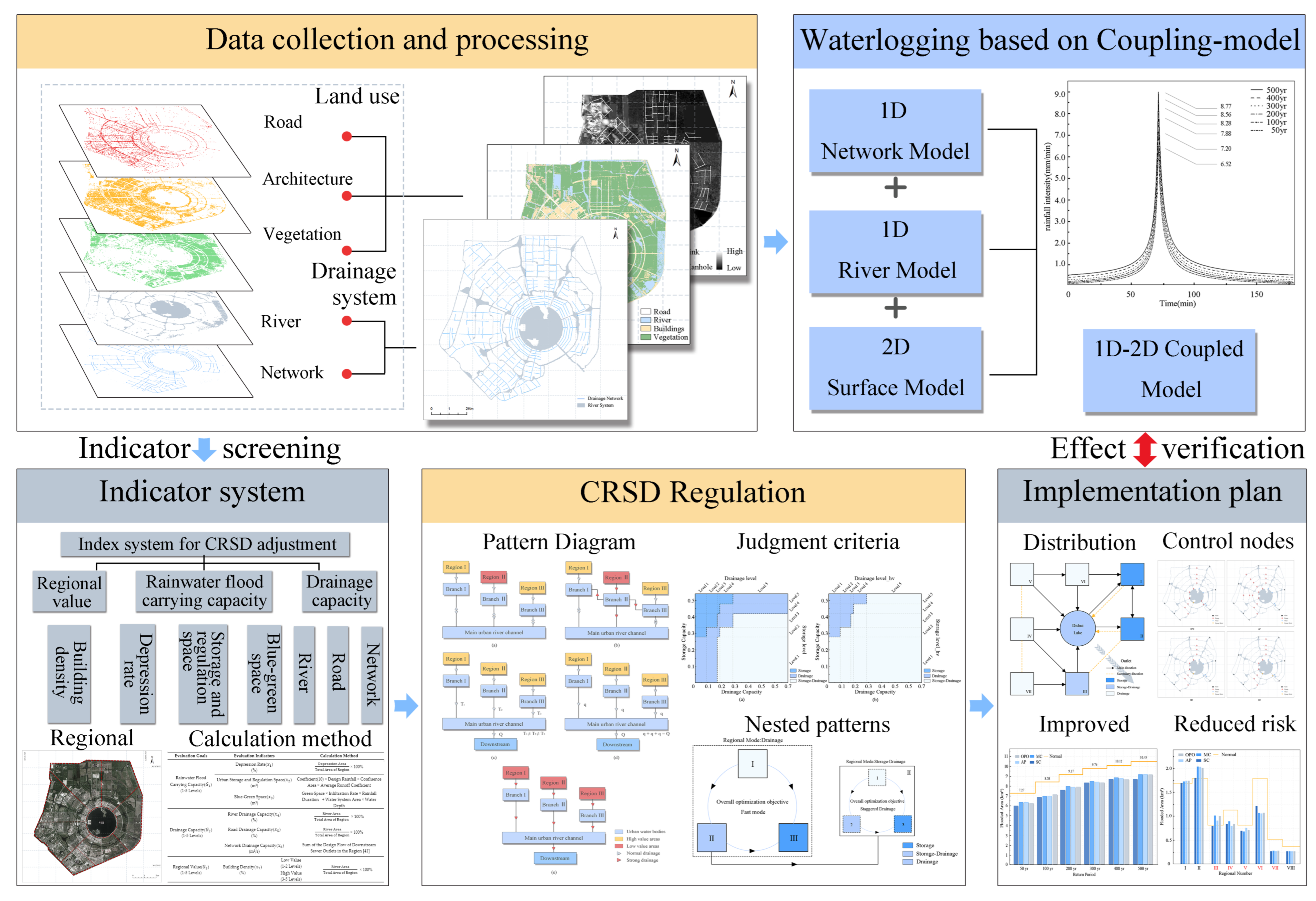
• Section 2 details the data sources and hydrological model construction for the case study area, introduces the CRSD framework, including its evaluation system, regional mode allocation rules, and optimization objectives.
• Section 3 analyzes the performance of CRSD under different rainfall return periods, compares optimization objectives, and evaluates waterlogging reduction effects through spatial distribution and downstream pressure metrics.
• Section 4 examines the applicability of CRSD strategies, interprets hydraulic mechanisms behind optimization outcomes, and discusses limitations in balancing regional priorities and infrastructure constraints.
• Section 5 summarizes the effectiveness of CRSD in enhancing urban flood resilience, highlights its innovation in cross-regional coordination, and proposes future research directions.

2. Materials and Methods

This study gathers regional data and selects key indicators to develop a CRSD evaluation system. Based on this system, CRSD rules are formulated to assess regional capabilities and assign corresponding models. A regional hydrological model is also constructed using the collected data. These CRSD principles are then applied to determine control methods, simulate the effects of CRSD under various scenarios, and compare the results with those from scenarios without CRSD to validate the model’s effectiveness. The entire process is illustrated in Figure 1.

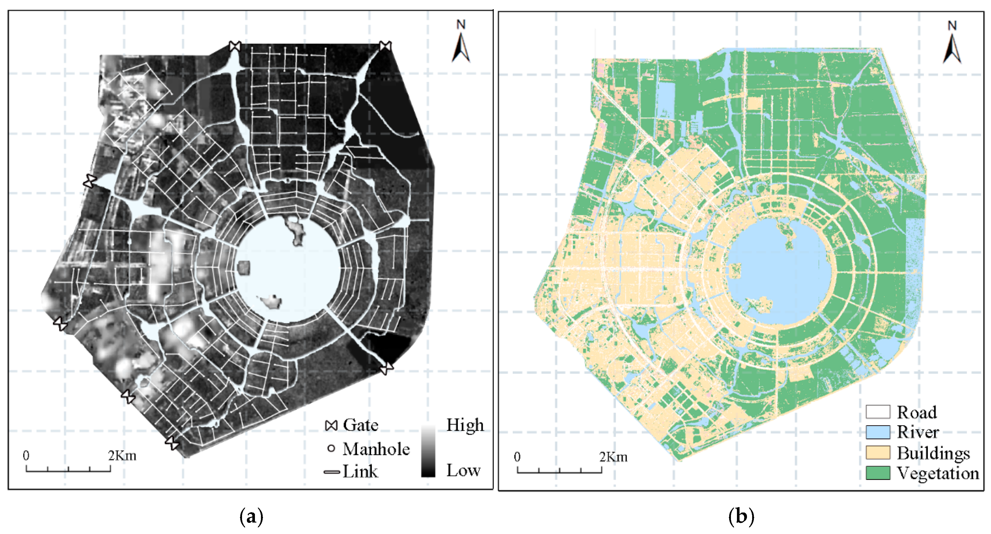
2.1. Regional Model Construction

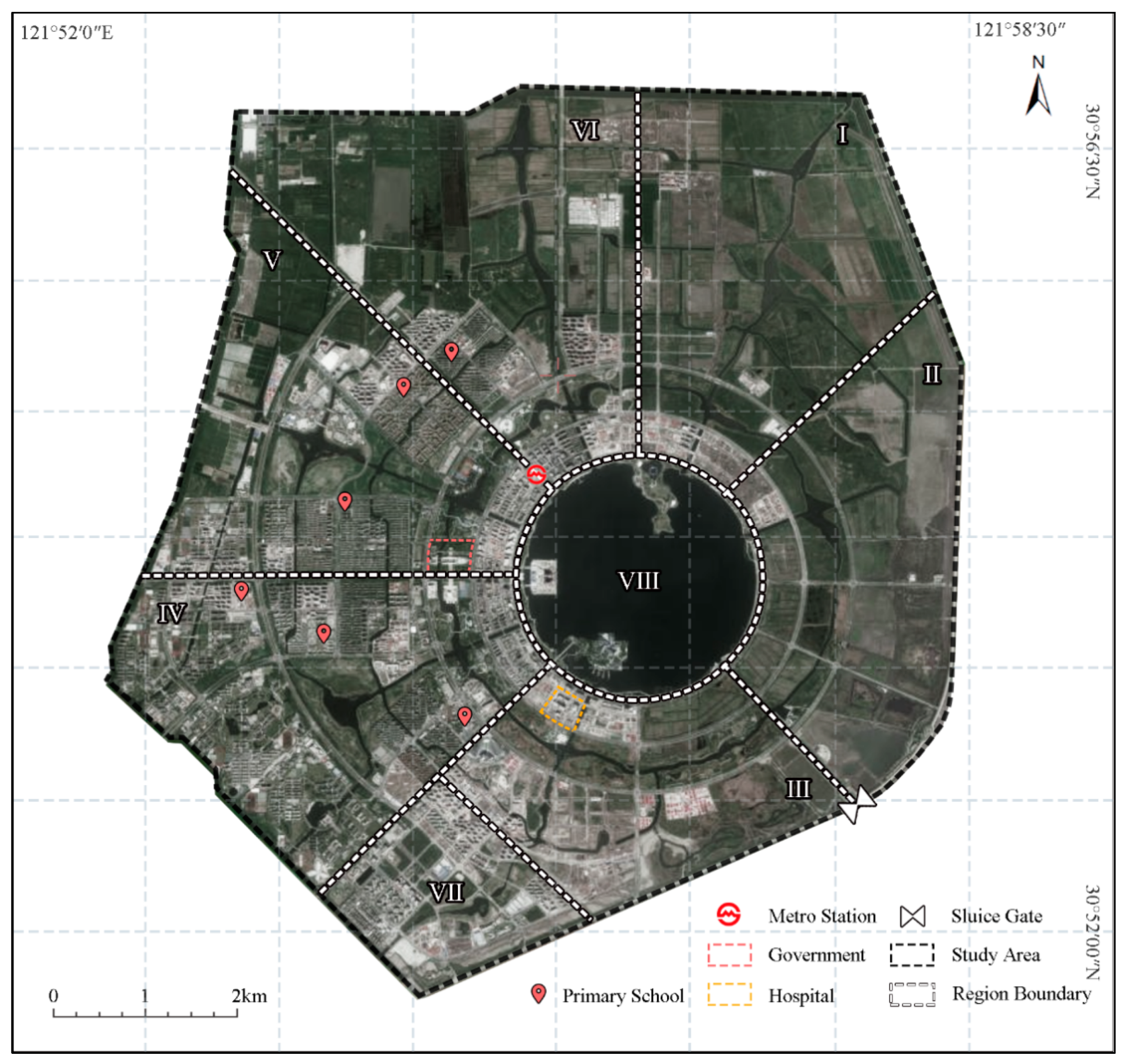
2.1.1. Regional Overview

The Dishui Lake area, located in the Lingang New Area of Shanghai, lies south of the Dazhi River and east of Jinhui Port, covering an area of 68.2 km². Surrounded by rivers, the area features control gates at key river mouths, forming a relatively isolated embanked zone. Centered around Dishui Lake, the region is characterized by four interconnected rivers and seven radial rivers. The terrain has a slope of less than 3%, with flat land and low surface runoff dynamics, typical of a plain city. Shanghai’s subtropical monsoon climate makes the Dishui Lake area particularly susceptible to extreme rainfall events (EREs), it is representative to select this area for research. The area is divided into eight relatively independent Subregions (I–VIII) based on drainage zoning (Figure 2).

The drainage system employs a separate approach for sewage and stormwater drainage. The river’s normal water level is 2.6 m, with the downstream area connected to the East China Sea via a single discharge sluice. Detailed hydrological information is provided in

Table 1. Regional hydrological information.

Composition	Name	Estuary Width (m)	Riverbed Width (m)	Riverbed Elevation (m)	Control Width (m)	Remarks
One Lake	Dishui Lake	--	--	--	--	Area: 4.5 km2
Four Rivers	Chunlian	43	15	−1	20	Partial Expansion Water level: 2.0–3.3 m
	Xialian	25–43	5–15	−1	20 (10)
	Qiulian	25–43	5–15	−1	20 (30)
	Donglian	25–43	5–15	−1	20 (6)
Seven Channels	Chifeng Channel	70	40	−1	30	--
	Chenghe Channel	30–45	15	−1	6–30	Partial Expansion Water level: 2.0–3.3 m
	Huangri Channel	45	15	−1	6–30
	L1ha Channel	45	15	−1	6–30
	Qingxiang Channel	45–90	15–60	−1	6–30
	Lanyun Channel	45	15	−1	30 (15)
	Zifei Channel	45	15	−1	30
Discharge Sluice	Dishui Lake Sluice	--	--	--	--	Maximum flow rate: 40 m3/s

.

2.1.2. Data Sources

This study utilizes Digital Elevation Model (DEM) data obtained from the Geographic Information Data Cloud Platform http://www.gscloud.cn (accessed on 1 October 2024). Due to confidentiality restrictions on drainage network data, the actual network parameters could not be accessed. Therefore, the drainage network topology is designed according to the 5-year return period standard. Although this method cannot accurately capture the hydraulic characteristics of the drainage network, the primary focus of this study is on extreme rainfall events (EREs), during which the network’s capacity is limited. Crucially, the absence of drainage network data does not compromise the validity of comparative effectiveness evaluations between CRSD scenarios, as all simulations maintain identical parameterization frameworks. The core research objective—assessing relative performance improvements through CRSD implementation—remains unaffected by this assumption.

In recent years, various coupled models have been applied to urban waterlogging simulations, accurately identifying the locations, extent, and waterlogging depth of stormwater overflow [37,38]. This study develops a waterlogging coupling model using MIKE FLOOD, with the drainage network comprising 420 pipe segments, 421 manholes, and 84 outfalls (Figure 3a), as well as the river network consisting of 4 tributaries and 7 main streams. Given that the highest resolution of the available DEM is 30 m, the 2D surface hydrodynamic model employs a 30 m × 30 m grid with closed boundary conditions. The area is then classified into four categories—roads, buildings, green spaces, and water bodies, based on land use data from the project (Figure 3b). According to project survey data, buildings in the area are typically taller than three stories. To simplify the representation of their impact on water flow, the building height is uniformly increased by 10 m, and road elevations are adjusted downward by 0.15 m to reflect curb height.

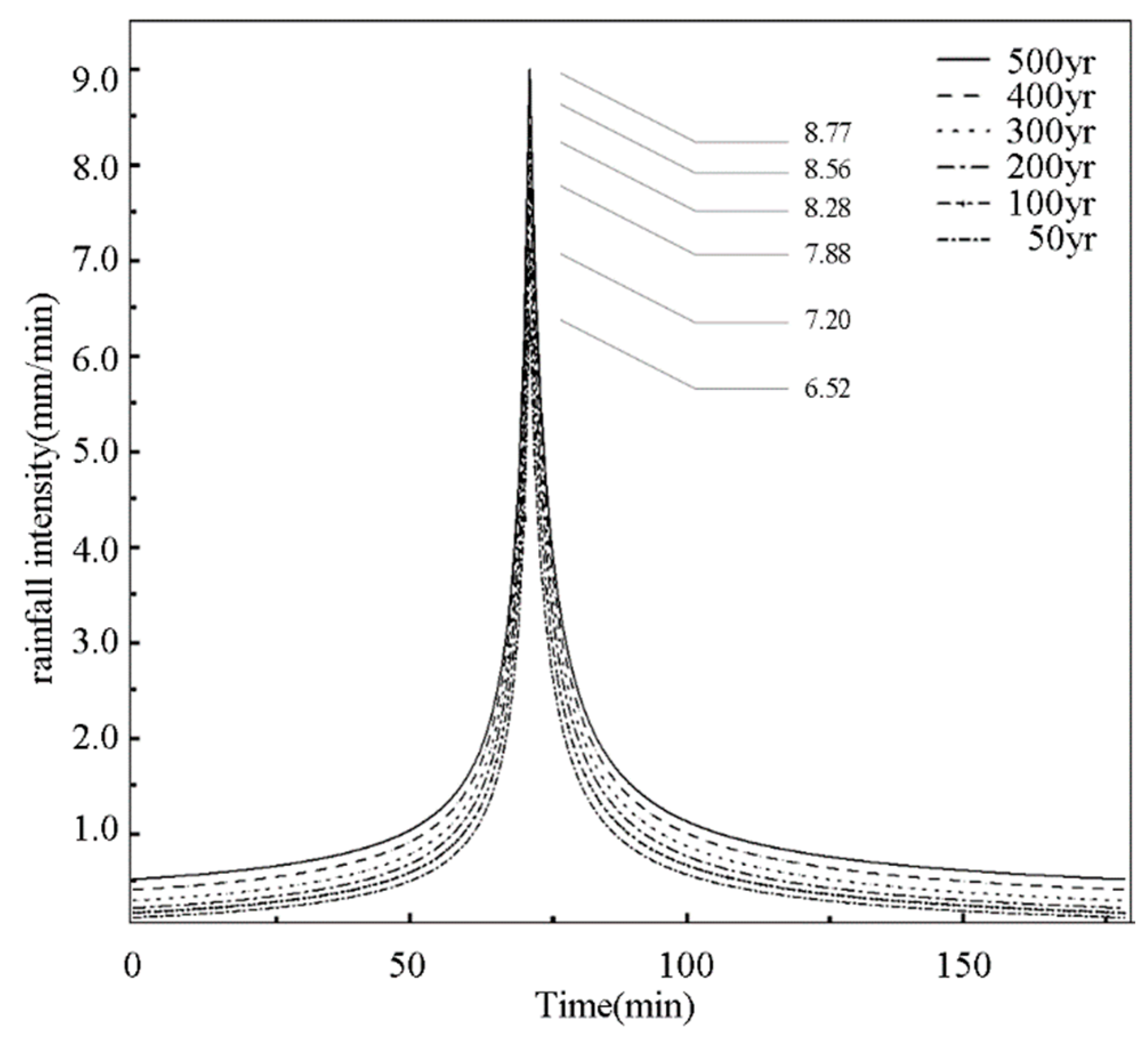
2.1.3. Design Rainfall

Research indicates that 75% of urban waterlogging disasters are caused by rainfall events lasting approximately 3 h [37]. This study uses the Shanghai Rainstorm Intensity Formula to construct EREs, with return periods ranging from 50 yr to 500 yr for short-duration rainfall events (with a duration of 3 h). According to the local standards of Shanghai (DB31/T 1043-2017), the peak rain coefficient is set to 0.4 to generate the design rainfall process curve (Figure 4).

The heavy rainfall intensity formula is shown as follows:

$$i={\displaystyle \frac{9.581(1+0.846lgP)}{{(t+7.0)}^{0.656}}},$$

(1)

In the formula: $i$ is the rainfall intensity (unit: mm/min); $t$ is the rainfall duration (unit: min); $P$ is the rainfall return period (unit: a).

To quantitatively assess the waterlogging control effectiveness of CRSD, the urban waterlogging risk in this study was divided into three levels: 0.15 cm ≤ mild waterlogging (level 1); ≤0.3 m < moderate waterlogging (level 2); <0.5 m ≤ severe waterlogging (level 3) waterlogging [14,39].

2.2. Establishment of CRSD

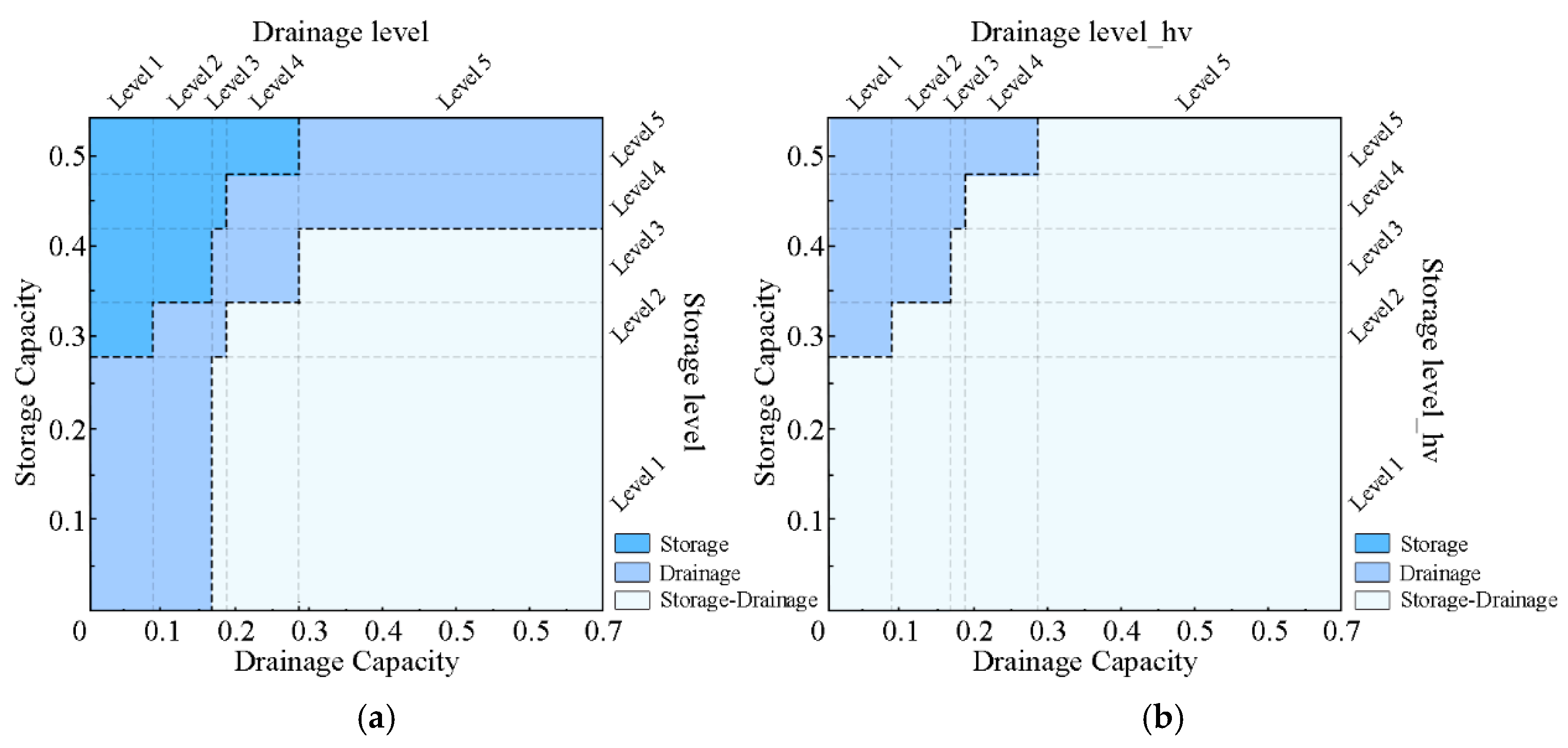
2.2.1. Regional Allocation of CRSD

The entropy weight method, an objective numerical assignment technique, uses entropy value theory to determine the weight of each influencing factor’s indicators. This approach eliminates subjective bias, allowing for a more accurate reflection of each factor’s importance in the comprehensive evaluation of impact targets [40]. The evaluation system for CRSD is constructed based on the entropy weight method [41]. In the mode selection process, it is crucial to thoroughly consider the region’s water storage and drainage capacity, socio-economic conditions, and ecological factors [42]. Therefore, this study selects indicators across three dimensions: rainwater waterlogging carrying capacity, drainage capacity, and regional value. The natural breaks method is employed to categorize each indicator into five levels (1–5). The specific indicator framework and calculation methods are provided in the table below (

Table 2. Indicator evaluation system and calculation methods for CRSD in plain cities.

Evaluation Goals	Evaluation Indicators		Calculation Method
$\mathrm{Rainwater} \mathrm{Flood} \mathrm{Carrying} \mathrm{Capacity} \left(G_1\right)$ (1–5 Levels)	$\mathrm{Depression} \mathrm{Rate} (x_1$) (%)		${\displaystyle \frac{\mathrm{D}\mathrm{e}\mathrm{p}\mathrm{r}\mathrm{e}\mathrm{s}\mathrm{s}\mathrm{i}\mathrm{o}\mathrm{n} \mathrm{A}\mathrm{r}\mathrm{e}\mathrm{a}}{\mathrm{T}\mathrm{o}\mathrm{t}\mathrm{a}\mathrm{l} \mathrm{A}\mathrm{r}\mathrm{e}\mathrm{a} \mathrm{o}\mathrm{f} \mathrm{R}\mathrm{e}\mathrm{g}\mathrm{i}\mathrm{o}\mathrm{n}}}$× 100%
	$\mathrm{Urban} \mathrm{Storage} \mathrm{and} \mathrm{Regulation} \mathrm{Space} \left(x_2\right)$ (m3)		Coefficient (10) × Design Rainfall × Confluence Area × Average Runoff Coefficient
	$\text{Blue-Green} \mathrm{Space} (x_3$) (m3)		Green Space × Infiltration Rate × Rainfall Duration + Water System Area × Water Depth
$\mathrm{Drainage} \mathrm{Capacity} (G_2$) (1–5 Levels)	$\mathrm{River} \mathrm{Drainage} \mathrm{Capacity} (x_4$) (%)		${\displaystyle \frac{\mathrm{R}\mathrm{i}\mathrm{v}\mathrm{e}\mathrm{r} \mathrm{A}\mathrm{r}\mathrm{e}\mathrm{a}}{\mathrm{T}\mathrm{o}\mathrm{t}\mathrm{a}\mathrm{l} \mathrm{A}\mathrm{r}\mathrm{e}\mathrm{a} \mathrm{o}\mathrm{f} \mathrm{R}\mathrm{e}\mathrm{g}\mathrm{i}\mathrm{o}\mathrm{n}}}$ × 100%
	$\mathrm{Road} \mathrm{Drainage} \mathrm{Capacity} (x_5$) (%)		${\displaystyle \frac{\mathrm{R}\mathrm{o}\mathrm{a}\mathrm{d} \mathrm{A}\mathrm{r}\mathrm{e}\mathrm{a}}{\mathrm{T}\mathrm{o}\mathrm{t}\mathrm{a}\mathrm{l} \mathrm{A}\mathrm{r}\mathrm{e}\mathrm{a} \mathrm{o}\mathrm{f} \mathrm{R}\mathrm{e}\mathrm{g}\mathrm{i}\mathrm{o}\mathrm{n}}}$ × 100%
	$\mathrm{Network} \mathrm{Drainage} \mathrm{Capacity} (x_6$) (m3/s)		Sum of the Design Flow of Downstream Sewer Outlets in the Region [43]
$\mathrm{Regional} \mathrm{Value} (G_3$) (1–5 Levels)	$\mathrm{Building} \mathrm{Density} (x_7$) (%)	Low Value (1–2 Levels)	${\displaystyle \frac{\mathrm{R}\mathrm{i}\mathrm{v}\mathrm{e}\mathrm{r} \mathrm{A}\mathrm{r}\mathrm{e}\mathrm{a}}{\mathrm{T}\mathrm{o}\mathrm{t}\mathrm{a}\mathrm{l} \mathrm{A}\mathrm{r}\mathrm{e}\mathrm{a} \mathrm{o}\mathrm{f} \mathrm{R}\mathrm{e}\mathrm{g}\mathrm{i}\mathrm{o}\mathrm{n}}}$ × 100%
		High Value (3–5 Levels)

Note(s): The depression rate is defined as the percentage of low-lying terrain area within a specific region relative to the total area of that region. For simplicity, the proportion of regional road area and the proportion of regional river channel area are used as substitute indicators to assess road drainage capacity and river drainage capacity. Building area is used as a generalization of regional value.

).

The calculation of the regional rainwater flood carrying capacity, drainage capacity, and regional value is provided below:

$$G_k={\sum }_{i=m}^n{\mathrm{w}}_i\times {\displaystyle \frac{x_i-x_{i min}}{x_{i max}}}$$

(2)

In the formula: $G_k$ is the final quantity of the k-th evaluation goals; ${\mathrm{w}}_i$ is the weight of the i-th indicator in the evaluation indicator under the k-th evaluation goal; $x_i$ is the numerical value of the i-th indicator in the evaluation indicator under the k-th evaluation goal; $x_{i max}$ and $x_{i min}$ represent the maximum and minimum values of the i-th indicator

The basic CRSD modes are categorized into three types: priority storage, priority drainage, and combined storage and drainage. For high-value regions, priority should be given to drainage, while for regions with lower value but better ecological conditions, measures should focus on alleviating flood pressure in high-value areas [44]. Figure 5 illustrates the mode selection rules for low-value and high-value regions (HV). In this figure, the horizontal axis represents drainage capacity, and the vertical axis represents rainwater flood carrying capacity. The value ranges (level 1 to level 5) based on the natural breaks method are presented in

Table 3. Range of classification levels.

Evaluation Goals	Level 1	Level 2	Level 3	Level4	Level 5
$G_1$	0–0.28	0.28–0.34	0.34–0.42	0.42–0.48	0.48–0.52
$G_2$	0–0.09	0.09–0.17	0.17–0.19	0.19–0.29	0.29–0.71
$G_3$	0–0.11	0.11–0.25	0.25–0.32	0.32–0.64	0.64–1.11

.

Figure 5 presents the regional mode selection chart. By comparing three key indicators, the appropriate regional mode can be determined. For low-value regions (Figure 5a), the priority storage mode is applied when the rainwater flood carrying capacity exceeds the drainage capacity. Conversely, if the rainwater flood carrying capacity is at least two levels lower than the drainage capacity, the priority drainage mode is chosen. If both capacities are similar, the combined storage and drainage mode is adopted.

For high-value regions (Figure 5b), the priority drainage strategy is generally preferred to rapidly address waterlogging. The combined storage and drainage mode is only used when the rainwater flood carrying capacity surpasses the drainage capacity. In all other cases, the priority drainage mode is implemented.

For example, if Region A is categorized as a low-risk area, the model selection follows Figure 5a. When the rainwater carrying capacity is at level 3 (0.34–0.42) and the drainage capacity is at level 1 (0–0.09), the region falls within the deep blue area. Therefore, the model for Region A would prioritize water storage.

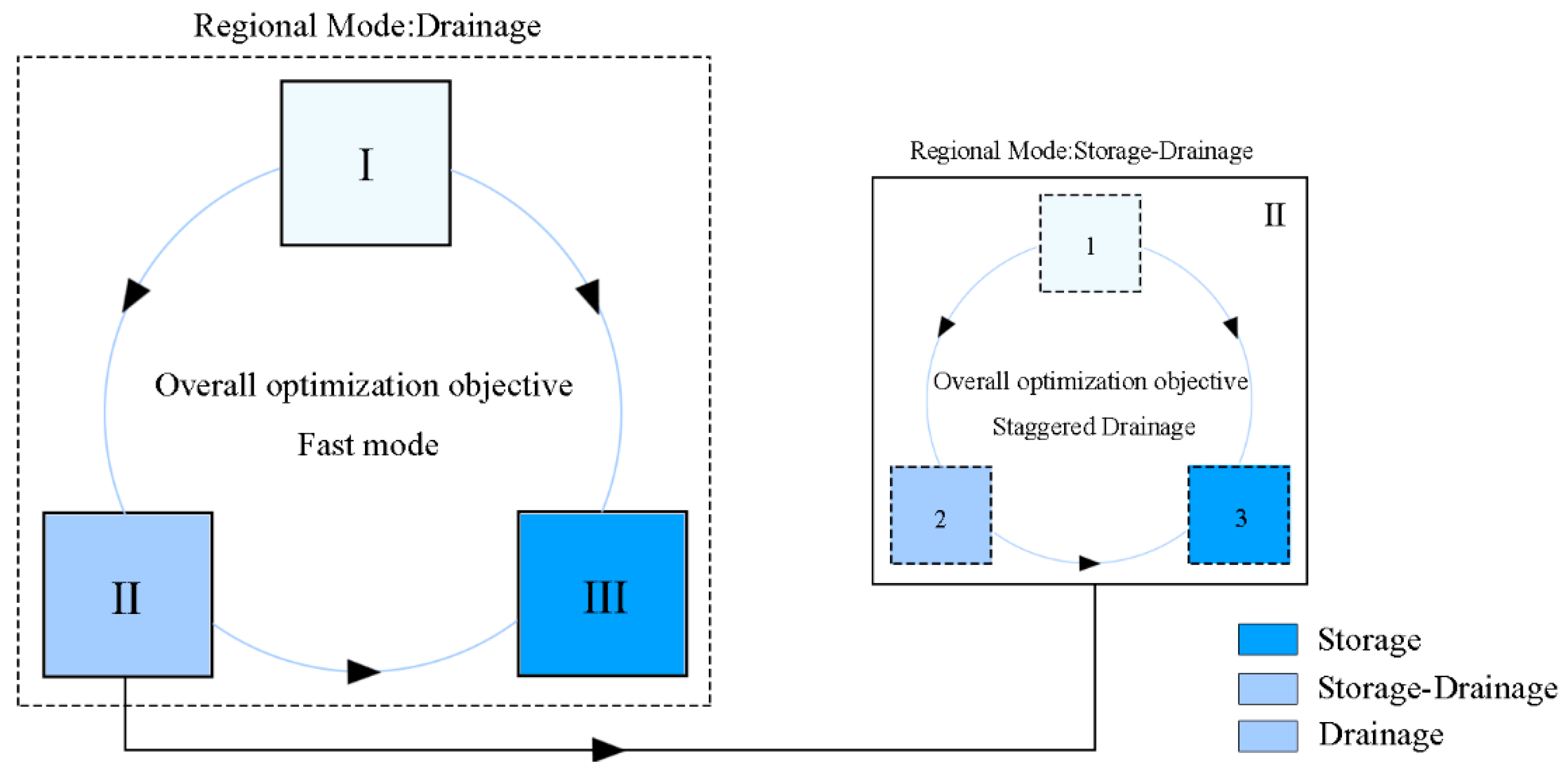
2.2.2. Scheduling Rules of CRSD

CRSD strategy alleviates the contradiction between the demand for rainwater management space and the insufficient urban space through inter-regional water volume scheduling [36]. Establishing scheduling rules can clarify the water distribution path to address the above issue. The specific rules include:

• Watershed Principle: CRSD implementation is only allowed within the same watershed.
• Upstream–Downstream Principle: Water from upstream regions can be preferentially stored and regulated into downstream regions;
• Value Principle: High-value regions should prioritize drainage to low-value regions;
• Mode Principle: The drainage priority among different modes is priority drainage > combined storage and drainage > priority storage.
• Carrying Capacity Principle: Regions with lower rainwater flood carrying capacity can drain into regions with higher carrying capacity.
• Rule Priority: The priority of the rules is: Mode Principle > Value Principle > Carrying Capacity Principle > Upstream–Downstream Principle
• When the drainage priorities of regions are the same, they can drain into each other.

It should be clarified that this model is not a multi-objective optimization model, but rather a strategy selection process based on a single objective, focusing on choosing the most appropriate storage and drainage mode according to the specific characteristics and needs of the region.

2.2.3. Optimization Objective of CRSD

Setting targeted optimization objectives can enhance the coordination and cooperation among regions. The following five optimization objectives are proposed, and the user can select them according to the specific conditions of the region and the surrounding areas.

• Maximum Consumption (MC): Maximize the retention of excess rainfall within the urban river network system, which may increase waterlogging risks in high-value regions;
• Safe Consumption (SC): Prioritize the safety of high-value regions, using low-value regions for storage and regulation;
• Off-Peak Outflow (OPO): Through mutual cooperation between regions, avoid runoff peaks occurring simultaneously in downstream discharge areas;
• Average Pressure (AP): Adjust the storage and discharge ratio between regions to ensure that the river levels in regions with the same mode are consistent;
• Rapid Drainage (RD): Achieve rapid rainwater discharge by improving the convergence capacity of sewer networks and lowering upstream water levels, thereby mitigating the damming effect.

The relationship between the optimization objectives and the basic CRSD modes (Figure 6) is illustrated as follows: The dashed box on the left represents the overall area, which is subdivided into three subregions (I–III). Subregions I–III correspond to the priority water storage area, priority drainage area, and combined water storage and drainage area, respectively. These subregions work in coordination to achieve the optimization goals defined by the user. Furthermore, each subregion can be further divided. For instance, Subregion II can be broken down into Subregions I–III, corresponding to the priority water storage area, priority drainage area, and combined water storage and drainage area, respectively. The coordination among these subregions facilitates the achievement of Subregion II’s overall optimization goals. This nested subdivision method ensures the effective implementation of top-down water storage and drainage planning at a specified scale.

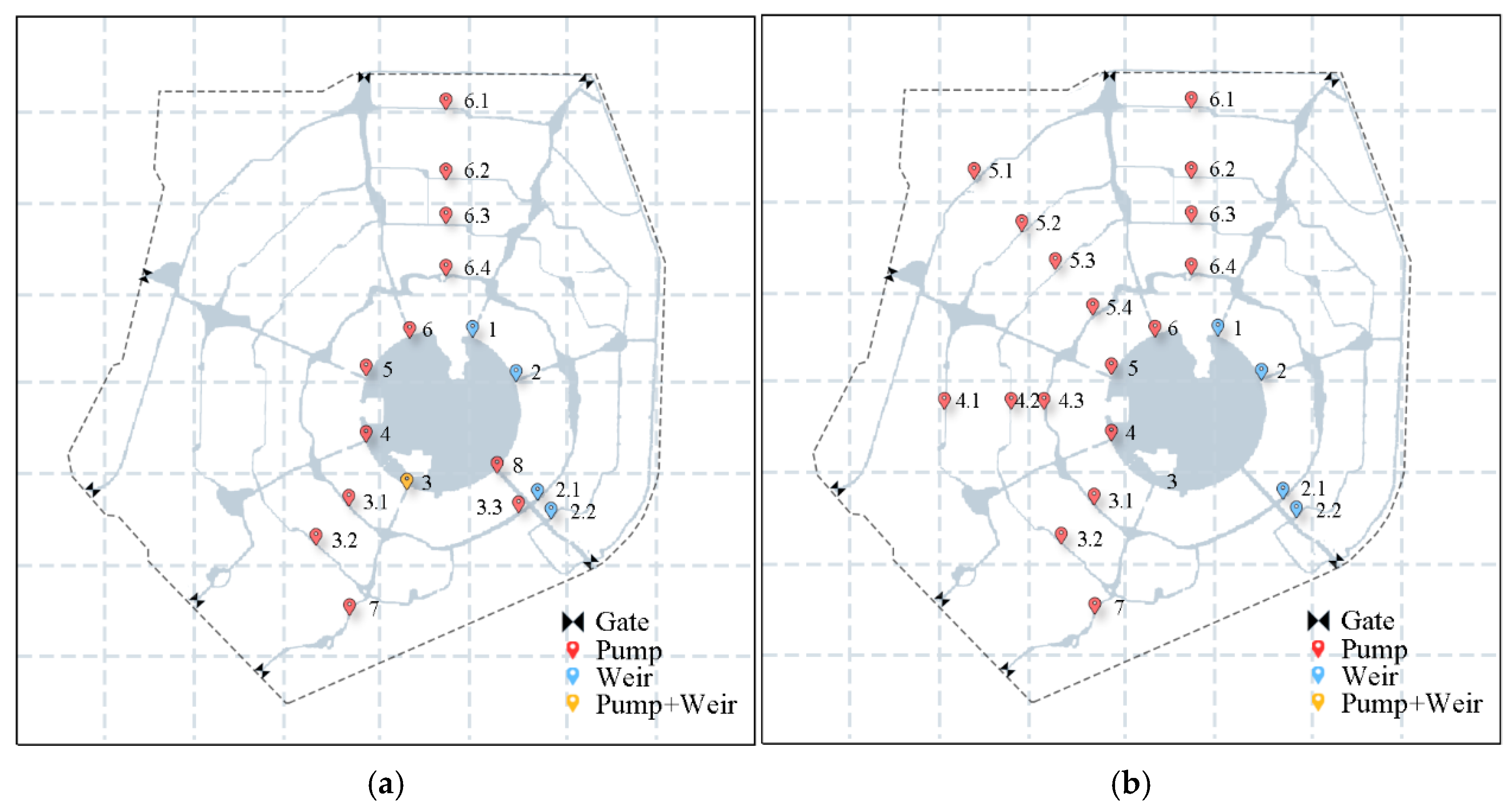
2.2.4. Control Methods of CRSD

Urban drainage systems face higher waterlogging risks due to issues such as insufficient inlet points, defects in the network topology, and low confluence efficiency [45,46]. Simulation results indicate that when the pump station capacity is 3.5 m³/s, the regional drainage network utilization reaches its maximum. Further increases in pump station capacity do not effectively improve drainage efficiency (Figure 7).

CRSD enhances the confluence capacity of drainage networks in priority drainage and combined storage-drainage regions by installing pumps at key inspection well nodes (Figure 8a). Additionally, in line with CRSD principles and optimization objectives, hydraulic control facilities such as pumping stations, overflow weirs, and sluice gates are deployed in rivers (Figure 8b). By dynamically adjusting river water levels, the CRSD method strengthens the city’s flood control capacity in the context of extreme rainfall events (EREs).

2.3. Evaluation Indicators for CRSD Effectiveness

To visually assess the effectiveness of CRSD in flood prevention and control within the study area, this study selects several key indicators, including the rate of change in waterlogging area, reduction in waterlogging area, waterlogging point distribution, density, and changes in downstream outlet water levels. Specifically, the waterlogging area change rate reflects the rate at which waterlogging areas change over time or under different scenarios. It evaluates the effectiveness of CRSD by comparing the waterlogging areas before and after implementation and assessing the speed of change. The reduction in waterlogging area quantifies the decrease in waterlogging extent by measuring the difference in waterlogging areas before and after CRSD implementation, helping to evaluate the actual impact of CRSD on controlling waterlogging. The distribution and density of waterlogging points describe the spatial distribution of waterlogging points within the study area and their concentration levels. Distribution refers to the specific areas where waterlogging points are concentrated, while density measures the number of waterlogging points within a given area. A higher density of waterlogging points generally indicates more severe drainage issues in that area, which may require additional mitigation measures. Changes in downstream outlet water levels measure variations in water levels at the downstream drainage outlets. The implementation of CRSD can influence the flow of water throughout the watershed, and changes in downstream water levels reflect CRSD’s impact on the overall water resource distribution and drainage system. A decrease in downstream water levels suggests that CRSD has effectively reduced the flow of water downstream, alleviating waterlogging problems. The calculation formulas for some of the indicators are shown as follows.

The reduced waterlogging area and waterlogging area change rate are calculated using the following formula:

$$R={\displaystyle \frac{\Delta A}{A_0}}\times 100\%$$

(3)

$$\Delta A=A_1-A_0$$

(4)

In the formula, $R$ represents the waterlogging change rate, $\Delta A$ represents the reduced waterlogging area, $A_1$ represents the waterlogging area after the change, and $A_0$ represents the waterlogging area before the change.

The waterlogging point density is calculated using the following formula:

$$f’\left(x\right)={\displaystyle \frac{1}{nh}}\sum _{i=m}^{n}K\left({\displaystyle \frac{x-x_i}{h}}\right)$$

(5)

In the formula, $f’\left(x\right)$ is the waterlogging point density estimate at point $x$, $n$ is the total number of waterlogging points, $h$ is the bandwidth parameter, $x_i$ is the i-th waterlogging point, and $K$ is the kernel function, typically the Gaussian kernel.

3. Results

3.1. Results of CRSD

3.1.1. Indicator Weights and Regional Modes

Based on the calculation methods for the indicators outlined above, the weights of each indicator were determined using the entropy weight method (

Table 4. Final weights of each indicator.

Evaluation Goals	Evaluation Indicators	Weight
$G_1$	$x_1$	0.21
	$x_2$	0.27
	$x_3$	0.15
$G_2$	$x_4$	0.70
	$x_5$	0.21
	$x_6$	0.09
$G_3$	$x_7$	1

). The analysis reveals that the blue–green space has the most significant impact on urban rainwater flood carrying capacity, while river drainage capacity plays a decisive role in evaluating regional drainage capacity.

$G_1$$x_1$$x_2$$x_3$$G_2$$x_4$$x_5$$x_6$$G_3$$x_7$ The evaluation results for each region, based on the indicator system, are presented in

Table 5. Regional evaluation results.

Region No.	${\mathit{G}}_1$	${\mathit{G}}_2$	${\mathit{G}}_3$	Regional Mode
I	Level 2	Level 1	Level 2	Priority Storage
II	Level 4	Level 3	Level 2	Priority Storage
III	Level 3	Level 2	Level 4	Storage Discharge
IV	Level 3	Level 4	Level 5	Priority Discharge
V	Level 3	Level 4	Level 5	Priority Discharge
VI	Level 3	Level 3	Level 3	Priority Discharge
VII	Level 1	Level 2	Level 3	Priority Discharge
VIII	Level 5	Level 5	Level 1	Storage Discharge

. The indicator score represents the weighted score for each dimension.

3.1.2. Water Allocation of CRSD

Based on the above evaluation results and the basic CRSD principles, the drainage paths between regions have been determined (Figure 9). In this figure, dark blue blocks represent the priority storage mode, light blue blocks represent the combined storage and drainage mode, and white skyblue blocks represent the priority drainage mode. Square symbols denote Regions I to VII, while circular symbols represent Drip Water Lake. Gray arrows indicate river sections directly connected to downstream drainage sluice gates, while line segments represent interconnected paths between regions. The direction of the arrows indicates the water flow direction. Black arrows represent the primary drainage direction, while orange arrows indicate the secondary drainage direction. Taking Region V as an example, according to the watershed principle, Region V is interconnected with Regions IV, VI, and VIII for water resource allocation; according to the drainage mode principle, Region V should drain into Drip Water Lake; according to the value mode, although Regions IV and VI share the same mode as Region V, due to their higher value, drainage from Region V may be directed to Regions IV and VI. Finally, based on the priority ranking of these principles, Region V and Drip Water Lake are designated as the primary drainage path, while Regions IV and VI serve as the secondary drainage path.

The drainage paths between regions and their respective priorities are presented in

Table 6. Regional drainage pathway.

Source Region	Target Region	Flow Type
I	II	Free Flow
	VIII	Opportunistic Drainage
II	III	Disconnected
	VIII	Opportunistic Drainage
III	VIII	Priority Drainage
IV	III	Priority Drainage
	VIII	Priority Drainage
V	IV	Free Flow/Opportunistic Drainage
	VI	Free Flow/Opportunistic Drainage
	VIII	Priority Drainage
VI	I	Priority Drainage
	VIII	Priority Drainage
VII	III	Priority Drainage
VIII	I	Priority Drainage
	II	Priority Drainage
	Outlet	Priority Drainage

.

3.1.3. Optimization Objective Control Scheme

The study area is composed of independent polders, and its connection to the outlet is solely through the Dishi Lake sluice, rendering the RD method unsuitable for this region. In the absence of external constraints, however, the RD model can enhance regional drainage efficiency and reduce the extent of waterlogging. In accordance with the fundamental principles of CRSD, appropriate hydraulic facilities should be strategically placed along the primary drainage paths to establish the desired drainage direction. Furthermore, selectively positioning hydraulic facilities along secondary drainage paths can further support the implementation of the CRSD model. These hydraulic facilities adjust in real-time based on river water levels, enabling coordinated operation across both drainage pathways to achieve diverse optimization objectives (Figure 9).

In OPO (Figure 10a), Regions I–II prioritize the collection of rainwater from Regions IV to VI through nodes 6.1–6.4 and stop accepting rainwater when the river capacity of Regions I–II reaches its maximum (water level ≥ 3.3 m). Meanwhile, Region III discharges rainwater downstream through node 3.3, while Region VIII discharges rainwater downstream through node 8 when the flood peak arrives. Regions III and VIII cooperate closely through nodes 3.3 and 8 to ensure that the downstream discharge does not experience the cumulative effect of flood peaks.

In AP (Figure 10b), Regions I–II collect rainwater from Regions IV–VI through nodes 6.1–6.4, while Regions IV–VI balance the river water levels of all three regions through nodes 4.1–5.3. At the same time, node 3 connects Region III and Region VIII to jointly bear the storage and discharge pressure.

In MC (Figure 10c), all regions except for Regions IV–VI are required to store water. Region III collects rainwater from Regions IV–VI through nodes 3.1–3.2 and node 7, and when the water level exceeds 3.3 m, Region III discharges water to Region VIII.

Unlike MC, SC (Figure 10d) stores water according to the importance of each region. Regions I–II collect rainwater from Regions IV–VI through nodes 6.1–6.4, while Regions IV–VI are required to prioritize discharging water to Region VIII through nodes 4–6. If the water level in Region VIII exceeds 3.3 m, nodes 4–6 are closed, and other regions assist in water storage. The types of nodes and their operation priorities are shown in the table below (

Table 7. Node control methodology.

Optimization Objective	Facility Type	Location ID	Control Method
OPO	Pump	6.1–6.4	Open if the water level before the pump in Region VI is greater than 2.1 m and the water level in Region I is less than 3.3 m, otherwise close.
		4–7	Open if the water level before the pump in Region IV-VII is greater than 2.1 m, otherwise close.
		3.1–3.2	Open if the water level before the pump in Region IV is greater than 2.1 m and the water level in Region III is less than 3.3 m, otherwise close.
		3	Open if the water level in Region III is greater than 3.2 m, otherwise close.
		8	Keep open to maintain downstream water level around 2.6 m.
	Gate	3.3	Keep open to maintain downstream water level around 2.6 m.
	Weir	All	Open during rainfall, with a height restriction of 3.3 m.
AP	Pump	6.1–6.4	Open if the water level before the pump in Region VI is greater than 2.1 m and the water level in Region I is less than 3.3 m, otherwise close.
		4–7	Open if the water level before the pump in Region IV–VII is greater than 2.1 m, otherwise close.
		4.1–4.3, 5.1–5.4	Maintain consistent water levels in Regions IV–VI.
		3.1–3.2	Open if the water level before the pump in Region IV is greater than 2.1 m and the water level in Region III is less than 3.3 m, otherwise close.
	Weir	All	Open during rainfall, with a height restriction of 3.3 m.
MC	Pump	6.1–6.4	Open if the water level before the pump in Region VI is greater than 2.1 m and the water level in Region I is less than 3.3 m, otherwise close.
		4–7	Open if the water level before the pump in Region IV–VII is greater than 2.1 m, otherwise close.
		3	Open if the water level in Region III is greater than 3.2 m, otherwise close.
		3.1–3.2	Open if the water level before the pump in Region IV is greater than 2.1 m and the water level in Region III is less than 3.3 m, otherwise close.
	Weir	All	Open during rainfall, with a height restriction of 3.3 m.
SC	Pump	6.1–6.4	Open if the water level before the pump in Region VI is greater than 2.1 m, the water level in Region I is less than 3.3 m, and the water level in Dripping Water Lake is greater than 3.3 m, otherwise close.
		4–7	Open if the water level before the pump in Region IV–VII is greater than 2.1 m, otherwise close.
		3, 3.3	Open if the water level in Region III is greater than 2.1 m, and close when the water level in Dripping Water Lake is greater than 3.3 m.
		3.1–3.2	Open if the water level before the pump in Region IV is greater than 2.1 m and the water level in Region III is less than 3.3 m, otherwise close.
	Weir	All	Open during rainfall, with a height restriction of 3.3 m.

).

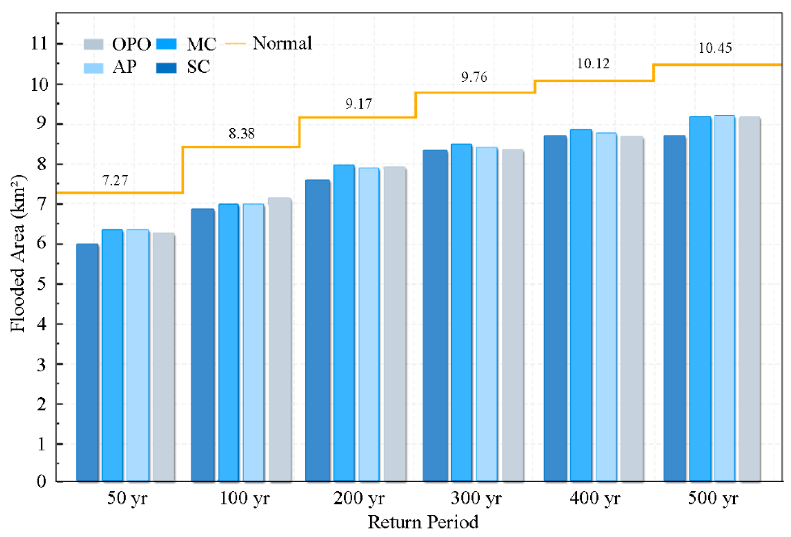
3.2. Mode Effect Evaluation Under Different Return Periods

3.2.1. Regional Waterlogging Situation

By comparing the simulated results of peak rainfall depth for 50 yr and 500 yr (Figure 11), it can be observed that the drainage capacity in the study area is severely inadequate when dealing with EREs with a gap of over 64%. High-value regions face significant waterlogging risk, with large areas at high risk of severe waterlogging. As the return period of rainfall increases, the spatial distribution of waterlogging caused by EREs shows no significant change. Waterlogging is mainly concentrated in urban streets, downstream river areas, and low-lying regions.

As the return period of rainfall increases, the area at risk of waterlogging expands significantly (Figure 12). When the return period increases from 50 yr to 100 yr, the growth rate of the submerged area reaches 13.19%, exhibiting rapid expansion. However, once the return period exceeds 100 yr, the growth rate slows down, decreasing from 8.69% to 3.36%. It is noteworthy that the proportion of area for each risk level remains relatively stable as the return period increases, with fluctuations consistently within a range of ±2%. The waterlogging area and its proportion for each return period are shown in the table below (

Table 8. F Waterlogging Area and Proportion.

Return Period	Level 1 (km2)	Proportion (%)	Level 2 (km2)	Proportion (%)	Level 3 (km2)	Proportion (%)	Total (km2)	Waterlogging Area in High-Value (km2)
50 yr	3.58	49.18	1.86	25.57	1.83	25.25	7.27	4.24
100 yr	4.10	48.96	2.13	25.48	2.14	25.56	8.38	4.90
200 yr	4.48	48.82	2.29	25.01	2.40	26.17	9.17	5.32
300 yr	4.73	48.45	2.48	25.41	2.55	26.14	9.76	5.55
400 yr	4.78	47.38	2.64	26.18	2.67	26.44	10.09	5.80
500 yr	4.99	47.71	2.68	25.67	2.78	26.62	10.45	5.89

).

3.2.2. Drainage Capacity Improvement

After applying the CRSD method, the drainage capacity of the study area improved across all return periods. The orange line represents the waterlogged area in the region without CRSD, while different colors correspond to the waterlogged areas under the four optimization objectives (Figure 13). The results indicate that CRSD effectively enhances the city’s drainage capacity. All four optimization objectives contribute to mitigating urban waterlogging risks caused by extreme rainfall events (EREs). Specifically, the waterlogged area in the 300 yr period decreased from 9.76 km² to an average of 8.38 km², which is comparable to the average waterlogged area in the 100 yr period without the model. Similarly, the waterlogged area in the 500 yr period reduced to an average of 9.17 km², which is comparable to the average waterlogged area in the 200 yr period without the model. Among the optimization modes, SC performs relatively well, while MC shows less favorable results.

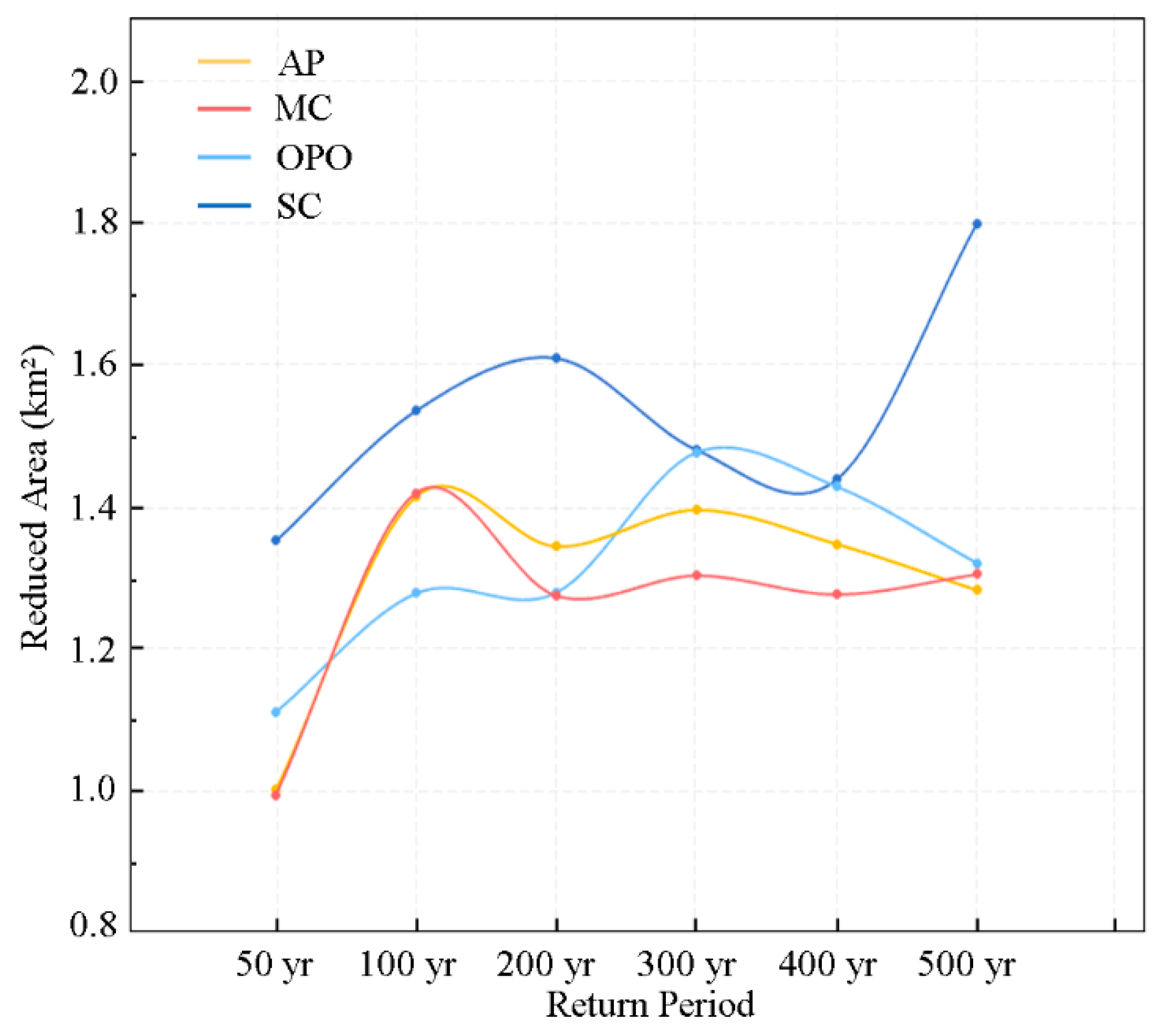
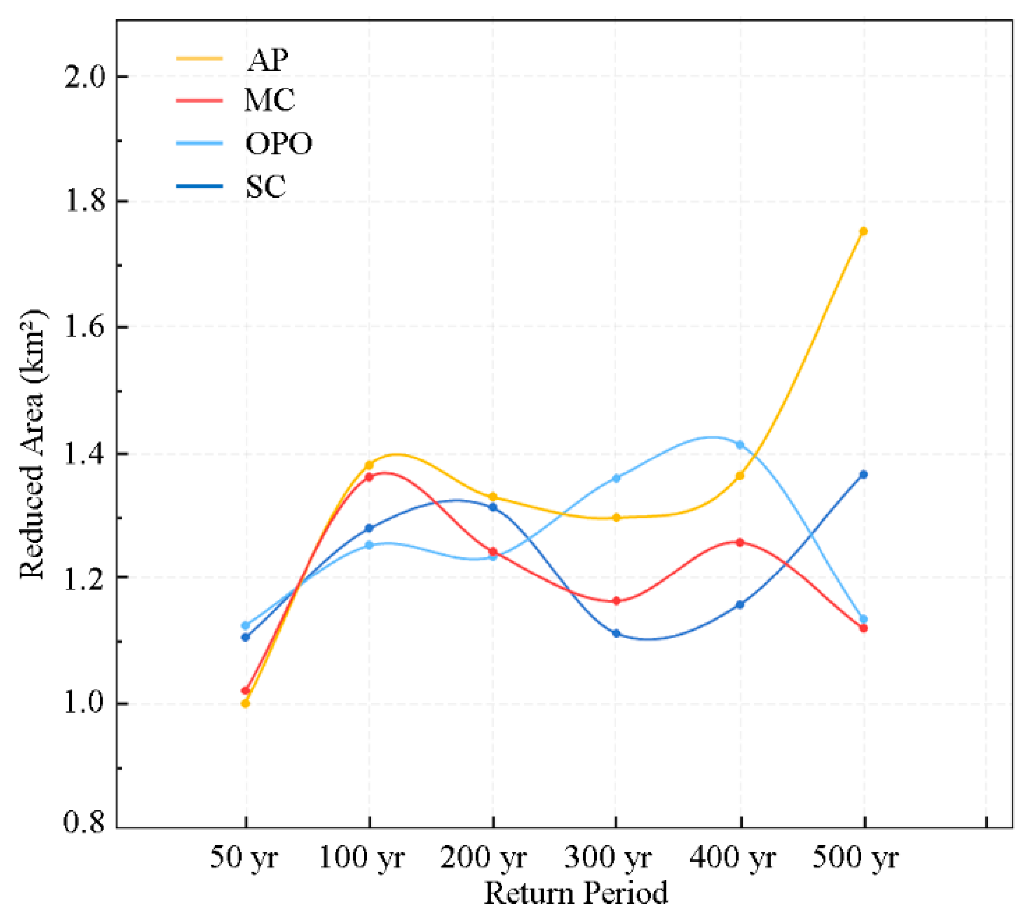
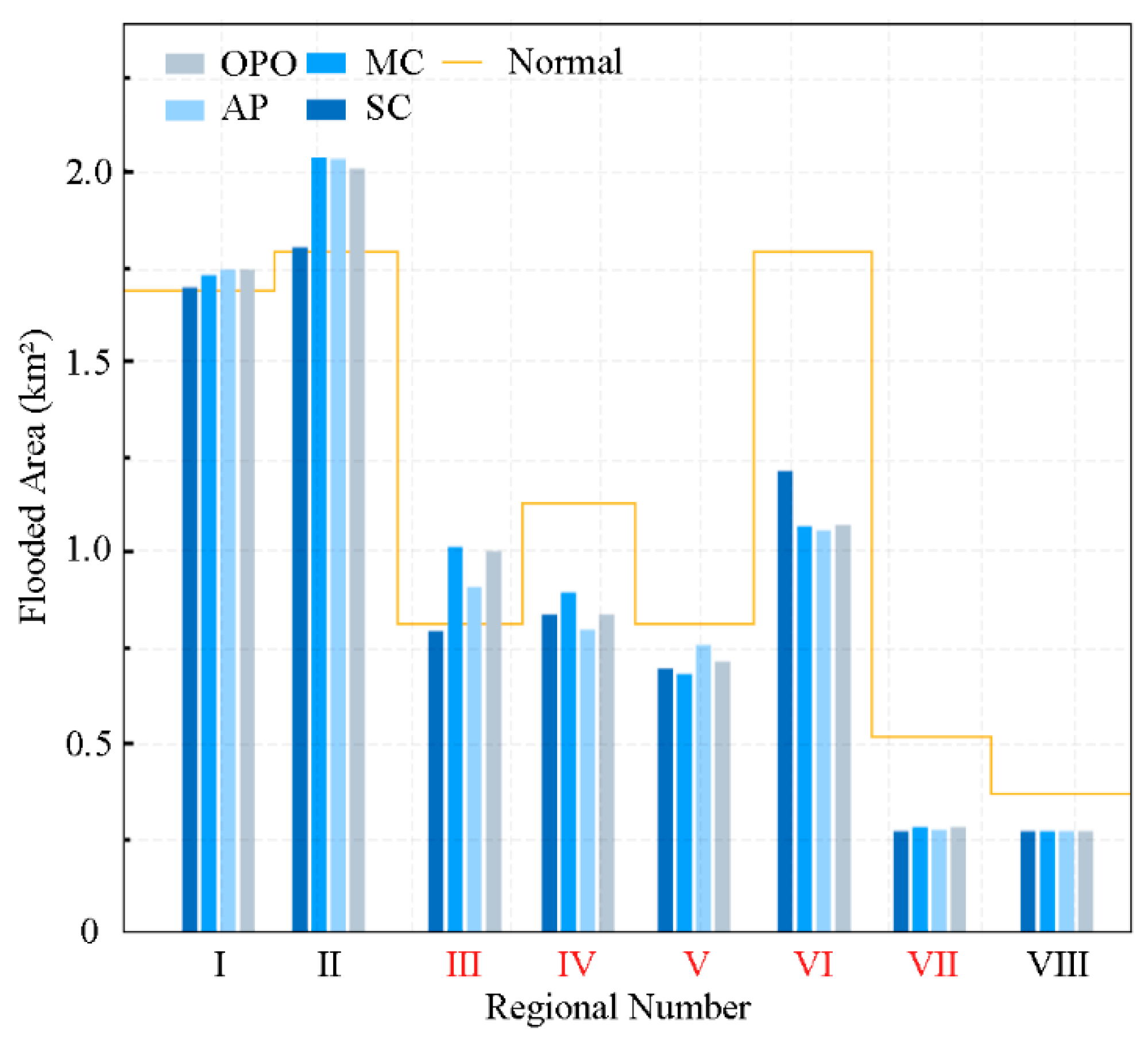
3.2.3. Comparison of Optimization Objectives’ Effects

Comparing the effects of different optimization objectives under various return periods (Figure 14), the results show that as the return period increases, the waterlogging mitigation effect of each optimization objective continues to improve during the early stages of rainfall (50 yr–100 yr). However, after 100 yr, the waterlogging mitigation effects of the optimizations exhibit significantly different trends as the return period increases. SC mode outperforms all other optimization objectives across all return periods. Its mitigation capacity continues to increase from 50 yr to 200 yr, reaching its peak at 200 yr. Subsequently, between 200 yr and 400 yr, the reduction in the waterlogged area gradually decreases, and the effect is most pronounced at 500 yr, where the waterlogged area is reduced by 1.80 km². MC and AP show rapid increases in waterlogging reduction in the early stages of rainfall, reaching their maximum values of 1.41 km² at 100 yr. However, after 100 yr, the waterlogging reduction area for both modes stabilizes. OPO exhibits a fluctuating upward trend across the 50 yr to 500 yr, with a maximum value of 1.47 km².

Comparing the effects of four waterlogging control modes on high-value areas under different rainfall return periods (Figure 15), the results show that during the early stages of rainfall (50 yr–100 yr), the waterlogging elimination effect increases rapidly. However, after 100 yr, the drainage capacity of each mode exhibits significantly different trends as the return period increases. AP continues to improve until it reaches its maximum value in 200 yr, then decreases slightly, with the best performance in 500 yr, eliminating 1.96 km² of waterlogged areas. MC shows a fluctuating downward trend after 100 yr, recovering only after 400 yr, and then declines again at 500 yr. OPO shows a fluctuating increasing trend from 50 yr to 400 yr, reaching its maximum value of 1.61 km² at 400 yr, before rapidly decreasing at 500 yr. SC shows a fluctuating upward trend from 50 yr to 500 yr, reaching its maximum value of 1.57 km² at 500 yr.

Comparing the waterlogging area in high-value regions with the waterlogging risk area across the entire case study area, it becomes evident that SC contributes significantly to the reduction in waterlogged areas in the overall study area, yielding relatively better results. However, its performance in reducing waterlogging in high-value regions is less notable. In contrast, AP shows the opposite trend: it performs well in mitigating waterlogging in high-risk areas, and as the return period increases, its effectiveness in reducing waterlogging risk in high-value regions becomes increasingly prominent.

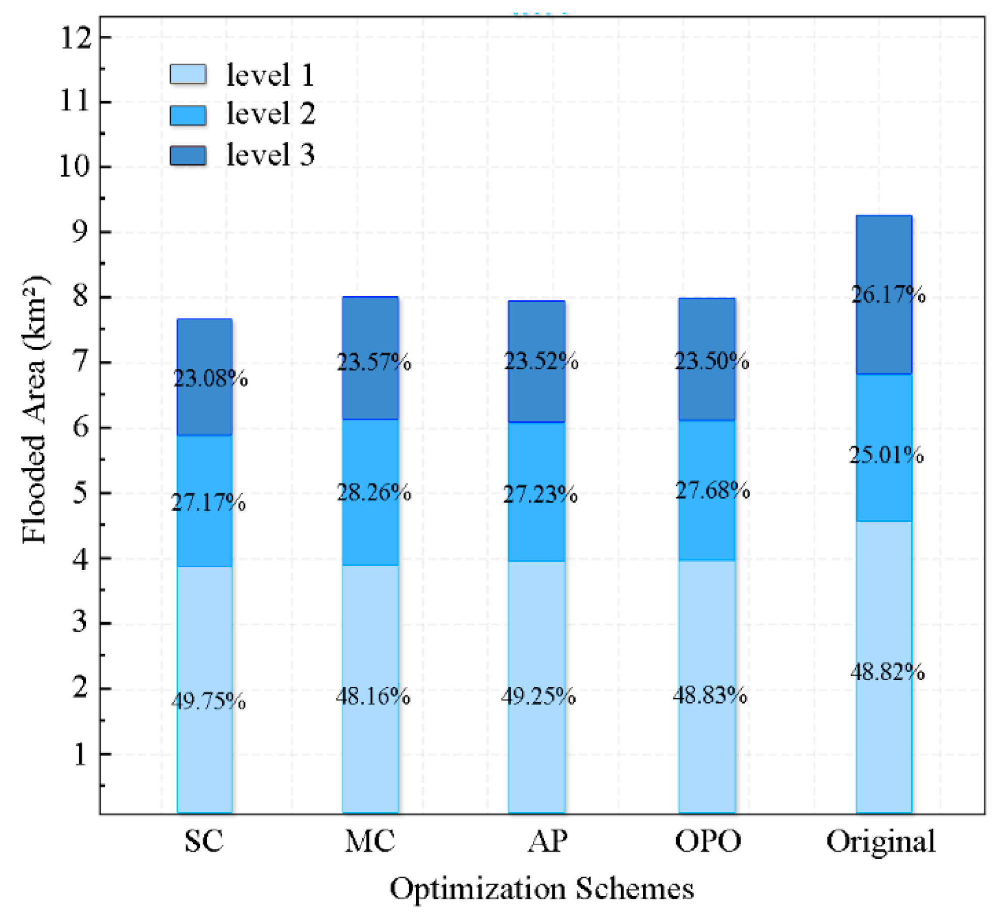
3.3. Evaluation of Mode Effects Under the Same Return Period—200 Yr

The design standards of urban flood control and drainage systems are generally focused on 50–100 yr. Using the 200 yr period can reveal the failure mechanisms of traditional systems under rainfall events exceeding the design standards. At the same time, the 200 yr period is considered a moderately high level within the return period range of 50 yr to 500 yr, possessing typical characteristics of extreme rainfall, yet not being too rare, thereby ensuring the practical feasibility of the research findings.

3.3.1. Comparison of Mode Effects

Comparing the simulation results of each optimization objective under the 200 yr period, by statistically analyzing the areas of different waterlogging levels and their proportions within the waterlogging area (Figure 16), the effectiveness of CRSD and the differences between optimization objectives are demonstrated. At 200 yr, SC shows the best waterlogging mitigation effect, reducing the waterlogged area by approximately 1.61 km². Additionally, it performs the best in reducing the proportion of severe waterlogging, with the severe waterlogging ratio decreasing from 26.17% to 23.08%.

The effects of different optimization objectives also vary among different regions. To showcase the comparison of waterlogging situations across various regions, the regions marked in red text represent the waterlogging situations in high-value areas (Figure 17). After implementing CRSD, all optimization objectives effectively reduce the waterlogging risk area in high-risk zones. Among them, SC not only ensures effective results but also has a minimal impact on other regions. AP demonstrates the best waterlogging mitigation effect, reducing the waterlogged area in high-value regions by 1.53 km².

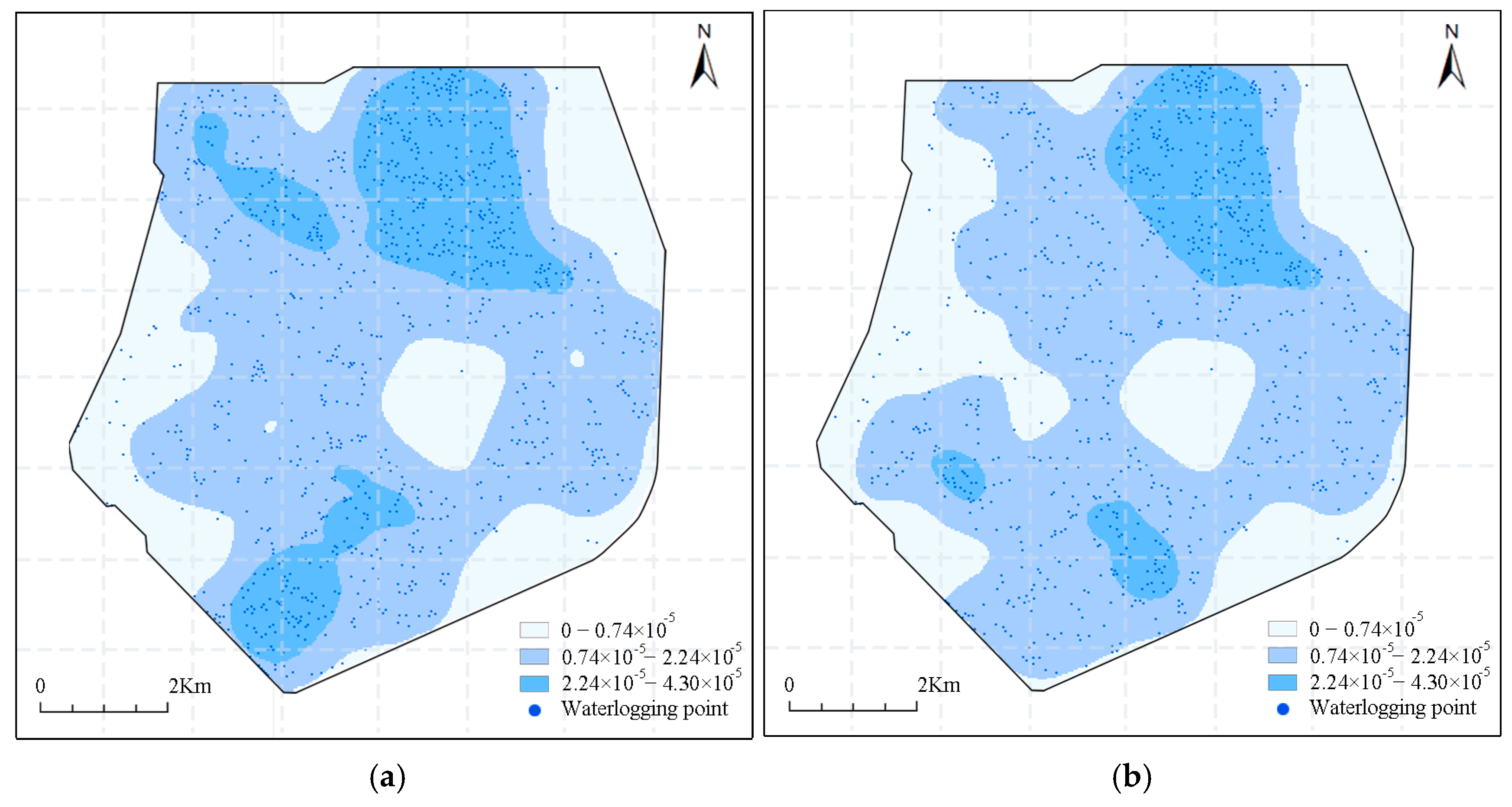
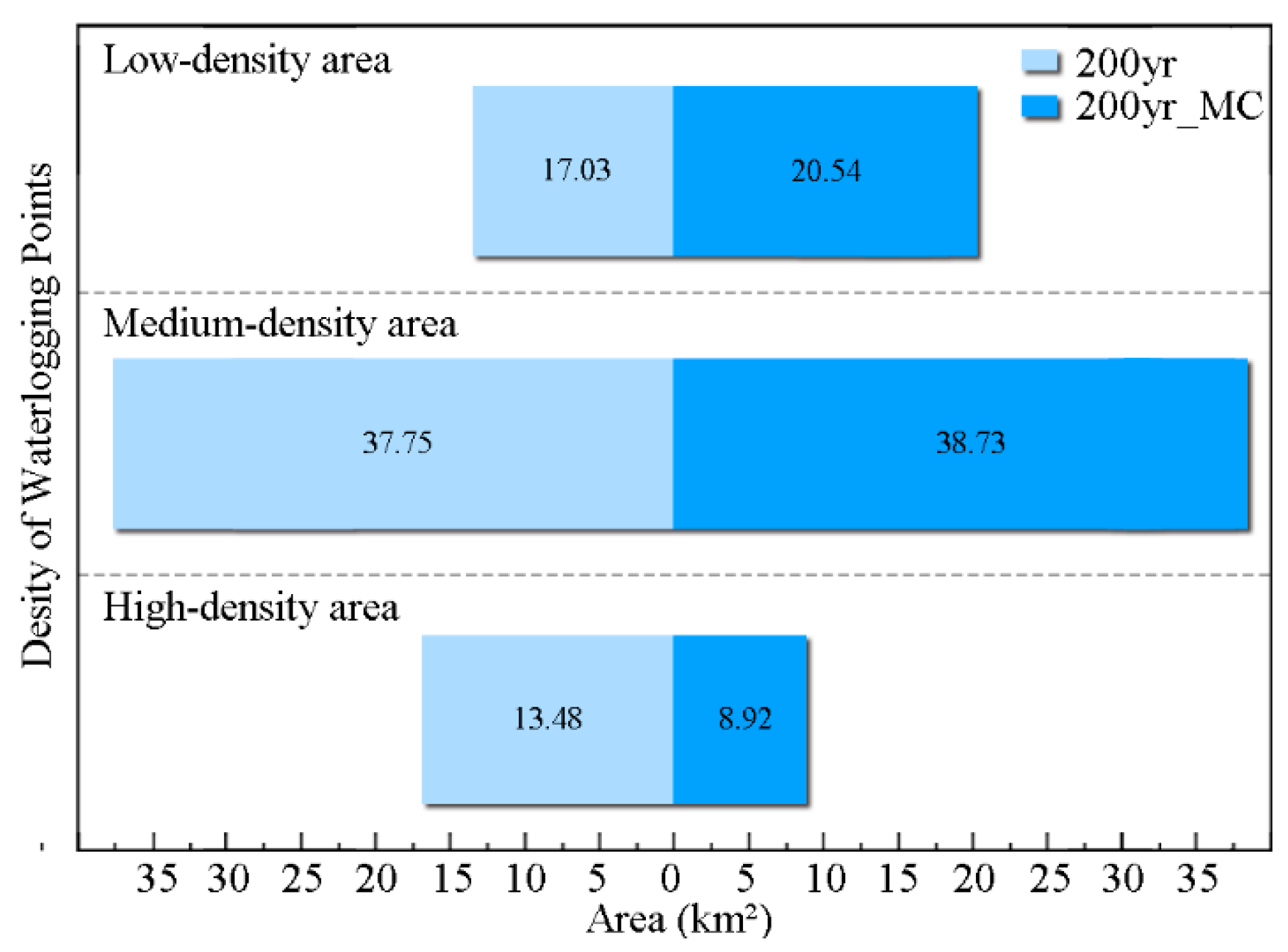
3.3.2. Waterlogging Point Density Distribution

By analyzing the number of waterlogging points under each mode and performing kernel density analysis (Figure 18), areas with darker shades indicate higher concentrations of waterlogging points. A higher density of waterlogging points in a given area typically correlates with lower drainage efficiency [14]. The analysis shows a total of 1059 waterlogging points in the region. After applying the CRSD method, the number of waterlogging points was significantly reduced, with the MC method yielding the best results, decreasing the number of points by 168. Furthermore, CRSD also reduced the extent of densely concentrated waterlogging points, shifting the high-density areas towards the eastern part of the study area (Figure 19).

3.3.3. Comparison of Outlet Pressure

Comparison of outlet water level under different modes at 200 yr (Figure 20). As shown in Figure 18, under normal conditions, the downstream outlet water level reaches its peak at around 4 h, with the peak water level approximately 1.73 m. When comparing the downstream outlet water levels under different modes, it can be seen that SC exerts the highest pressure on the downstream outlet, followed by AP and MC modes. OPO effectively controls the water level and reduces the downstream outlet pressure, with its peak water level not exceeding 1.8 m. Additionally, OPO can delay the peak time and reduce the peak flow.

4. Discussion

4.1. Evolution Characteristics of Urban Waterlogging Under EREs and Validation of CRSD Optimization System

In the context of EREs, the study area has experienced significant urban waterlogging. The waterlogged area increased from 7.27 km² to 10.45 km² as the return period extended from 50 yr to 500 yr (Table 8). At lower return periods, the flood area increases rapidly; however, the growth rate gradually slows down as the return period increases. This is because low-lying urban areas, which serve as the primary spaces to accommodate EREs, have already been fully utilized. As the return period increases further, only the flood depth can continue to increase. Additionally, the evaluation results (Figure 19) reveal that the waterlogged area in the prioritized drainage zones is relatively large, while the flood area in the prioritized storage zones remains smaller. Furthermore, the distribution of waterlogging points provides insight into regional drainage capacity: areas with lower densities of waterlogging points indicate stronger drainage capacity, while regions with higher densities correspond to weaker drainage capacity (Figure 17). These findings align with expectations and indirectly confirm the reliability of the CRSD evaluation system.

By highlighting the challenges posed by EREs to urban flood management, this study emphasizes the importance of optimizing drainage and storage strategies. It particularly affirms the reliability of the CRSD evaluation system, offering valuable guidance for the optimization of urban flood management systems.

4.2. Hydraulic Explanation of Response Curves

By comparing the response curves of various optimization objectives (Figure 13 and Figure 14), it can be seen that SC prioritizes the safety of high-value areas. It also utilizes a sluice-pump control system to preferentially direct floodwaters to low-value retention areas or downstream rivers. The scheme performs well when the river channel capacity is not fully utilized, but its effectiveness decreases when the return period exceeds 200 yr. However, the improvement in performance for 500 yr may be due to the high drainage pressure in high-value areas, which forces rainwater from other areas to be unable to flow into the river through the drainage network in the shortest possible time. As a result, more rainwater is absorbed by other facilities, indirectly increasing the capacity of the river channel.

MC prioritizes the use of storage spaces in low-value areas to maximize the interception of rainfall runoff. AP dynamically balances the water levels across multiple river sections through the pump station, ensuring that drainage pressure is evenly distributed across regions to prevent local flooding. At low return periods (50 yr–100 yr), regional storage capacity is sufficient, and the storage effect is significant, leading to a rapid reduction in water accumulation areas. However, as rainfall intensity increases, regional storage capacity becomes saturated and downstream river water levels rise, causing the effectiveness to gradually stabilize.

OPO by utilizing the temporal differences in drainage between regions, the scheme avoids overlapping with downstream flood peaks, reducing the instantaneous flow in the river. However, controlling downstream flood peaks weakens the drainage efficiency, and the existence of regional hydraulic response time differences leads to unstable performance under high return periods.

By comparing the strengths and weaknesses of each case, this study not only provides multiple feasible strategies for flood management but also offers scientific guidance for designing flood control solutions in different urban environments in the future.

4.3. Applicable Scenarios for Optimization Objectives

The results show that the effectiveness of the optimization objectives varies, each with its own limitations, making them suitable for different urban contexts. Specifically, the following observations can be made:

• SC prioritizes the protection of high-value areas while using low-value areas for water storage. Although the overall performance is good, this model results in a peak water level of 3.3 m at the downstream outlet, which increases the flood risk downstream. This model is suitable for urban areas with limited rainwater flood carrying capacity, where modifications are challenging, and the downstream flood risk is relatively low.
• MC maximizes the absorption of excess water by prioritizing water storage areas and the urban river network. However, due to the limited overall rainwater flood carrying capacity of the region, the model performs poorly under higher return periods. This model is suitable for urban areas with a higher rainwater flood carrying capacity.
• OPO reduces downstream flood pressure by implementing peak-shifting drainage; however, it sacrifices drainage efficiency during EREs. This model is suitable for urban areas with significant flood risk.
• AP balances the drainage pressure between high-value areas, reducing the waterlogged area in high-value zones by 1.96 km² and showing better performance under higher rainfall return periods. However, this model requires multi-region and multi-device coordinated scheduling, which increases system complexity. It is suitable for urban areas with a multi-center structure and good connectivity between regions.
• RD, though not discussed in this paper due to specific constraints, is expected to perform well in mitigating regional waterlogging. Its main disadvantage is the need for extensive hydraulic infrastructure, which increases costs. This model is suitable for cities with well-connected water systems and high-value areas.

These findings, through a comparison of different optimization schemes, reveal the advantages and limitations of each approach under different urban environments and flood risks. They provide scientific support for the design of future flood control strategies in various urban settings, especially in terms of their adaptability to different drainage capacities, regional structures, and hydraulic system conditions. These conclusions offer diverse perspectives and practical experience for urban flood management, with significant theoretical and practical value.

5. Conclusions

Extreme rainfall events (EREs) present significant challenges for flat, low-lying cities with inadequate surface runoff dynamics. Traditional grey infrastructure often experiences system overload when rainfall exceeds design thresholds, while the synergistic effectiveness of blue–green–grey integrated infrastructure is constrained by spatial conflicts and the lack of cross-regional coordination mechanisms. This study addresses these critical issues by proposing a Collaborative Regulation of Storage and Drainage (CRSD) system specifically designed for flat cities. By developing an entropy-weighted evaluation system that considers rainwater carrying capacity, drainage efficiency, and regional value, we have enabled differentiated allocation of storage and drainage strategies. The applicability of this system was validated using the MIKE coupled model. This approach enhances urban flood management by offering a replicable strategy for flat cities facing the increasing challenges posed by EREs. The key conclusions are as follows:

• In response to EREs, the study reveals a significant drainage deficit in the study area, with the drainage capacity falling short by over 64%. As the return period of rainfall increases, the waterlogged area develops in three distinct phases: a rapid rise, followed by a leveling off, and, ultimately, reaching a state of deep saturation. The implementation of CRSD can substantially mitigate urban waterlogging caused by EREs, with the capacity to absorb at least 0.98 km² of waterlogged area. Specifically, under a 500 yr return scenario, the waterlogged area is reduced to the level typically seen at 200 yr, and in the case of 300 yr, it is brought down to 100 yr.
• The CRSD evaluation system performs excellently in regional model assessments, as demonstrated by the waterlogging simulation results. The system identifies priority drainage areas, which are typically high-value regions with more severe waterlogging and weaker drainage capacity. In contrast, priority storage areas experience less severe waterlogging and are better equipped to manage excessive rainfall, highlighting the system’s ability to target and regulate critical areas effectively.
• CRSD model significantly improves urban waterlogging control by dynamically coordinating cross-regional water resource allocation with blue–green–grey infrastructure. In the scenario of a 500 yr return period, SC reduces waterlogged areas by 1.80 km², while AP reduces waterlogging by 1.96 km², particularly in high-value areas. This supports the effectiveness of regional differentiated regulation. The study also uncovers notable differences in the response mechanisms of various optimization objectives: SC optimizes conditions globally by prioritizing the safety of high-value areas, AP enhances resilience in high-risk zones by balancing pressure, and OPO alleviates downstream pressure through peak-shifting drainage techniques.

References

1. Kong, F.; Sun, S.; Lei, T.J. Understanding China’s Urban Rainstorm Waterlogging and Its Potential Governance. Water 2021, 13, 891. [Google Scholar] [CrossRef]
2. Ardiclioglu, M.; Hadi, A.; Periku, E.; Kuriqi, A. Experimental and Numerical Investigation of Bridge Configuration Effect on Hydraulic Regime. Int. J. Civ. Eng. 2022, 20, 981–991. [Google Scholar] [CrossRef]
3. Hosseini, F.S.; Choubin, B.; Mosavi, A.; Nabipour, N.; Shamshirband, S.; Darabi, H.; Haghighi, A.T. Flash-Flood Hazard Assessment Using Ensembles and Bayesian-Based Machine Learning Models: Application of the Simulated Annealing Feature Selection Method. Sci. Total Environ. 2020, 711, 135161. [Google Scholar] [CrossRef]
4. Zhou, X.Y.; Bai, Z.J.; Yang, Y.H. Linking Trends in Urban Extreme Rainfall to Urban Flooding in China. Int. J. Climatol. 2017, 37, 4586–4593. [Google Scholar] [CrossRef]
5. Kumar, S.; Kant, S.; Ahmed, R. Assessment of an Extreme Heavy Rainfall over Meghalaya, India on 16th & 17th June 2022: A Case Study Using Meteorological and Remote Sensing Observations. Trop. Cyclone Res. Rev. 2025, 14, 60–70. [Google Scholar] [CrossRef]
6. Saufina, E.; Trismidianto; Satiadi, D.; Harjupa, W.; Risyanto; Purwaningsih, A.; Fathrio, I.; Praja, A.S.; Juaeni, I.; Witono, A.; et al. The role of Madden-Julian Oscillation, Westerly Wind Bursts, and Kelvin Waves in Triggering Extreme Rainfall Through Mesoscale Convective Systems: A Case Study of West Sumatra, March 7–8, 2024. Atmos. Res. 2025, 318, 107993. [Google Scholar] [CrossRef]
7. Xie, C.; Xu, C.; Huang, Y.; Liu, J.; Shao, X.; Xu, X.; Gao, H.; Ma, J.; Xiao, Z. Advances in the Study of Natural Disasters Induced by the “23.7” Extreme Rainfall Event in North China. Nat. Hazards Res. 2025, 5, 1–13. [Google Scholar] [CrossRef]
8. Yazdanfar, Z.; Sharma, A. Urban Drainage System Planning and Design—Challenges with Climate Change and Urbanization: A Review. Water Sci. Technol. 2015, 72, 165–179. [Google Scholar] [CrossRef]
9. Tavakol-Davani, H.; Burian Steven, J.; Devkota, J.; Apul, D. Performance and Cost-Based Comparison of Green and Gray Infrastructure to Control Combined Sewer Overflows. J. Sustain. Water Built Environ. 2016, 2, 04015009. [Google Scholar] [CrossRef]
10. Zhang, Y.K.; Wang, E.S.; Gong, Y.W. A Structural Optimization of Urban Drainage Systems: An Optimization Approach for Mitigating Urban Floods. Water 2024, 16, 1696. [Google Scholar] [CrossRef]
11. Anwer, A.A.; Soliman, A.H.; Radwan, H.G. Hydraulic-Based Optimization Algorithm for the Design of Stormwater Drainage Networks. Appl. Water Sci. 2024, 14, 139. [Google Scholar] [CrossRef]
12. Ngamalieu-Nengoue, U.A.; Iglesias-Rey, P.L.; Martínez-Solano, F.J.; Mora-Meliá, D.; Valderrama, J.G.S. Urban Drainage Network Rehabilitation Considering Storm Tank Installation and Pipe Substitution. Water 2019, 11, 515. [Google Scholar] [CrossRef]
13. Mark, O.; Weesakul, S.; Apirumanekul, C.; Aroonnet, S.B.; Djordjević, S. Potential and Limitations of 1D Modelling of Urban Flooding. J. Hydrol. 2004, 299, 284–299. [Google Scholar] [CrossRef]
14. Ding, Y.; Wang, H.; Liu, Y.; Lei, X. Urban Waterlogging Structure Risk Assessment and Enhancement. J. Environ. Manag. 2024, 352, 120074. [Google Scholar] [CrossRef]
15. Lu, P.; Sun, Y.; Steffen, N. Scenario-Based Performance Assessment of Green-Grey-Blue Infrastructure for Flood-Resilient Spatial Solution: A Case Study of Pazhou, Guangzhou, Greater Bay Area. Landsc. Urban Plan. 2023, 238, 104804. [Google Scholar] [CrossRef]
16. Wang, J.; Liu, J.; Wang, H.; Shao, W.; Mei, C.; Ding, X. Matching Analysis of Investment Structure and Urban Inundation Control Function of Sponge Cities in China. J. Clean. Prod. 2020, 266, 121850. [Google Scholar] [CrossRef]
17. Wu, J.; Xu, J.; Lu, M.; Ming, H. An Integrated Modelling Framework for Optimization of the Placement of Grey-Green-Blue Infrastructure to Mitigate and Adapt Flood Risk: An Application to the Upper Ting River Watershed, China. J. Hydrol. Reg. Stud. 2025, 57, 102156. [Google Scholar] [CrossRef]
18. Chen, W.; Wang, W.; Huang, G.; Wang, Z.; Lai, C.; Yang, Z. The Capacity of Grey Infrastructure in Urban Flood Management: A Comprehensive Analysis of Grey Infrastructure and the Green-Grey Approach. Int. J. Disaster Risk Reduct. 2021, 54, 102045. [Google Scholar] [CrossRef]
19. Green, D.; O’Donnell, E.; Johnson, M.; Slater, L.; Thorne, C.; Zheng, S.; Stirling, R.; Chan, F.K.S.; Li, L.; Boothroyd, R.J. Green Infrastructure: The Future of Urban Flood Risk Management? Wiley Interdiscip. Rev. Water 2021, 8, e1560. [Google Scholar] [CrossRef]
20. Qin, Y. Urban Flooding Mitigation Techniques: A Systematic Review and Future Studies. Water 2020, 12, 3579. [Google Scholar] [CrossRef]
21. Wickenberg, B. Collaborating for Nature-Based Solutions: Bringing Research and Practice Together. Local Environ. 2024, 29, 118–134. [Google Scholar] [CrossRef]
22. Yin, D.; Zhang, X.; Cheng, Y.; Jia, H.; Jia, Q.; Yang, Y. Can Flood Resilience of Green-Grey-Blue System Cope with Future Uncertainty? Water Res. 2023, 242, 120315. [Google Scholar] [CrossRef] [PubMed]
23. Omori, Y.; Kuriyama, K.; Tsuge, T.; Onuma, A.; Shoji, Y. Coastal Infrastructure Typology and People’s Preference-Based Grey-Green-Hybrid Infrastructure Classifications Using a Latent Class Model: A Case Study of Japan. Int. J. Disaster Risk Reduct. 2024, 114, 104992. [Google Scholar] [CrossRef]
24. Sarkar, S.K.; Rahman, M.A.; Esraz-Ul-Zannat, M.; Islam, M.F. Simulation-Based Modeling of Urban Waterlogging in Khulna City. J. Water Clim. Change 2021, 12, 566–579. [Google Scholar] [CrossRef]
25. Alves, A.; Vojinovic, Z.; Kapelan, Z.; Sanchez, A.; Gersonius, B. Exploring Trade-Offs Among the Multiple Benefits of Green-Blue-Grey Infrastructure for Urban Flood Mitigation. Sci. Total Environ. 2020, 703, 134980. [Google Scholar] [CrossRef]
26. Zhi-Yong, H.; Xiao-Yan, H.E.; Jin-Chi, H.; Hui-Rang, W. Studing on Non-Engineering Flood Control Strategies Abroad (I): Disaster Reduction Measures. J. Nat. Disasters 2002, 5, 52–56. [Google Scholar]
27. Huang, X.; Shen, J.; Li, S.; Chi, C.; Guo, P.; Hu, P. Sustainable Flood Control Strategies Under Extreme Rainfall: Allocation of Flood Drainage Rights in the Middle and Lower Reaches of the Yellow River Based on a New Decision-Making Framework. J. Environ. Manag. 2024, 367, 122020. [Google Scholar] [CrossRef]
28. Zhang, J.; Zhang, C.; Liu, L.; Shen, J.; Zhang, D.; Sun, F. Necessity and Feasibility of Allocation and Trading of Drainage Rights in Jiangsu Province. Water Resour. Prot. 2019, 35, 25–28. [Google Scholar]
29. Liu, Q.; Yang, H.; Liu, M.; Sun, R.; Zhang, J. An Integrated Flood Risk Assessment Model for Cities Located in the Transitional Zone between Taihang Mountains and North China Plain: A Case Study in Shijiazhuang, Hebei, China. Atmosphere 2019, 10, 104. [Google Scholar] [CrossRef]
30. Zhang, Q.; Wu, Z.; Zhang, H.; Dalla Fontana, G.; Tarolli, P. Identifying Dominant Factors of Waterlogging Events in Metropolitan Coastal Cities: The Case Study of Guangzhou, China. J. Environ. Manag. 2020, 271, 110951. [Google Scholar] [CrossRef]
31. Wang, J.; Liu, J.; Mei, C.; Wang, H.; Lu, J. A Multi-Objective Optimization Model for Synergistic Effect Analysis of Integrated Green-Gray-Blue Drainage System in Urban Inundation Control. J. Hydrol. 2022, 609, 127725. [Google Scholar] [CrossRef]
32. Liu, Y.; Zhang, X.; Liu, J.; Wang, Y.; Jia, H.; Tao, S. A Flood Resilience Assessment Method of Green-Grey-Blue Coupled Urban Drainage System Considering Backwater Effects. Ecol. Indic. 2025, 170, 113032. [Google Scholar] [CrossRef]
33. Joyce, J.; Chang, N.-B.; Harji, R.; Ruppert, T. Coupling Infrastructure Resilience and Flood Risk Assessment via Copulas Analyses for a Coastal Green-Grey-Blue Drainage System Under Extreme Weather Events. Environ. Model. Softw. 2018, 100, 82–103. [Google Scholar] [CrossRef]
34. Lintsen, H. Two Centuries of Central Water Management in the Netherlands. Technol. Cult. 2002, 43, 549–568. [Google Scholar] [CrossRef]
35. Guo, J. Urban Flood Mitigation and Stormwater Management; CRC Press: Boca Raton, FL, USA, 2017. [Google Scholar]
36. Yau, W.K.; Radhakrishnan, M.; Liong, S.-Y.; Zevenbergen, C.; Pathirana, A. Effectiveness of Abc Waters Design Features for Runoff Quantity Control in Urban Singapore. Water 2017, 9, 577. [Google Scholar] [CrossRef]
37. Zhang, M.; Xu, M.; Wang, Z.; Lai, C. Assessment of the Vulnerability of Road Networks to Urban Waterlogging Based on a Coupled Hydrodynamic Model. J. Hydrol. 2021, 603, 127105. [Google Scholar] [CrossRef]
38. Martínez, C.; Vojinovic, Z.; Price, R.; Sanchez, A. Modelling Infiltration Process, Overland Flow and Sewer System Interactions for Urban Flood Mitigation. Water 2021, 13, 2028. [Google Scholar] [CrossRef]
39. GB 51222-2017; Technical Code for Urban Flooding Prevention and Control. Ministry of Housing and Urban-Rural Development: Beijing, China, 2017.
40. Wang, Y.; Li, Y.; Li, H.; Dang, W.; Zheng, A. Study on the Correlation Between Soil Resistivity and Multiple Influencing Factors Using the Entropy Weight Method and Genetic Algorithm. Electr. Power Syst. Res. 2025, 246, 111692. [Google Scholar] [CrossRef]
41. Xu, Y.; Wang, J. A Maximum-Entropy-Based Method for Alarm Flood Prediction. J. Process Control 2021, 107, 58–69. [Google Scholar] [CrossRef]
42. Zhang, D.; Shen, J.; Liu, P.; Zhang, Q.; Sun, F. Use of Fuzzy Analytic Hierarchy Process and Environmental Gini Coefficient for Allocation of Regional Flood Drainage Rights. Int. J. Env. Res. Public Health 2020, 17, 2063. [Google Scholar] [CrossRef]
43. Vatankhah, A.R. Analytical Solution of Gradually Varied Flow Equation in Circular Channels Using Variable Manning Coefficient. Flow Meas. Instrum. 2015, 43, 53–58. [Google Scholar] [CrossRef]
44. Zhang, D.; Shen, J.; Sun, F.; Liu, B.; Wang, Z.; Zhang, K.; Li, L. Research on the Allocation of Flood Drainage Rights of the Sunan Canal Based on a Bi-level Multi-Objective Programming Model. Water 2019, 11, 1769. [Google Scholar] [CrossRef]
45. Al-busaltan, S.; Kadhim, M.; Basim, K.; Alshammaa, G. Evaluating Porous Pavement for the Mitigation of Stormwater Impacts; IOP Publishing: Bristol, UK, 2021; Volume 1067. [Google Scholar]
46. Barreiro, J.; Santos, F.; Ferreira, F.; Neves, R.; Saldanha Matos, J. Development of a 1D/2D Urban Flood Model Using the Open-Source Models SWMM and MOHID Land. Sustainability 2022, 15, 707. [Google Scholar] [CrossRef]
Figure 1. Technical roadmap.
Water 17 01385 g001
Figure 2. Location map of Lingang New District.
Water 17 01385 g002
Figure 3. Regional data: (a) DEM and drainage network of the study area; (b) land use of the study area.
Water 17 01385 g003
Figure 4. Design rainstorm intensity curve.
Water 17 01385 g004
Figure 5. Regional storage and discharge mode distribution diagram: (a) normal area; (b) high-value area.
Water 17 01385 g005
Figure 6. Mode nesting diagram.
Water 17 01385 g006
Figure 7. Drainage network utilization at different pump station capacities.
Water 17 01385 g007
Figure 8. Schematic of key node locations: (a) pipeline network key node; (b) river network key node.
Water 17 01385 g008
Figure 9. Basic CRSD network diagram.
Water 17 01385 g009
Figure 10. Diagram of river network node locations and types under different optimization objectives: (a) OPO, (b) AP, (c) MC, (d) SC.
Water 17 01385 g010aWater 17 01385 g010b
Figure 11. Pre-renovation regional waterlogging situation: (a) 50 yr; (b) 500 yr.
Water 17 01385 g011
Figure 12. Waterlogging area and its variation ratio map.
Water 17 01385 g012
Figure 13. Comparison of waterlogging area under different optimization objectives.
Water 17 01385 g013
Figure 14. Comparison of waterlogging area reduction effect under different optimization objectives.
Water 17 01385 g014
Figure 15. Comparison of the effects of different optimization objectives on high-value areas.
Water 17 01385 g015
Figure 16. Comparison of waterlogging area under different optimization objectives for 200yr.
Water 17 01385 g016
Figure 17. Waterlogging situation in the region under different optimization objectives.
Water 17 01385 g017
Figure 18. Waterlogging point density distribution map: (a) 200 yr, (b) 200 yr MC.
Water 17 01385 g018
Figure 19. Comparison of areas with different waterlogging point densities.
Water 17 01385 g019
Figure 20. Downstream outlet water levels under different optimization goals.
Water 17 01385 g020