An Overview of Evapotranspiration Estimation Models Utilizing Artificial Intelligence

Abstract

Evapotranspiration (ET) has a significant role in various natural and human systems, such as water cycle balance, climate regulation, ecosystem health, agriculture, hydrological cycle, water resource management, and climate studies. Among various approaches that are employed for estimating ET, the Penman–Monteith equation is known as the widely accepted reference approach. However, the extensive data requirement of this method is a crucial challenge that limits its usage, particularly in data-scarce regions. Therefore, as an alternative approach, artificial intelligence (AI) models have gained prominence for estimating evapotranspiration because of their capacity to handle complicated relationships between meteorological variables and water loss processes. These models leverage large datasets and advanced algorithms to provide accurate and timely ET predictions. The current research aims to review previous studies addressing the application of the AI model in ET modeling under four main categories: neuron-based, tree-based, kernel-based, and hybrid models. The results of this study indicated that traditional models like the Penman–Monteith (PM) require extensive input data, while AI-based approaches offer promising alternatives due to their ability to model complex nonlinear relationships. Despite their potential, AI models face challenges such as overfitting, interpretability, inconsistent input variable selection, and lack of integration with physical ET processes, highlighting the need for standardized input configurations, better pre-processing techniques, and incorporation of hydrological and remote sensing data.

1. Introduction

Evapotranspiration (ET), a dual process encompassing evaporation (a physical phase) and transpiration (a biological phase), refers to the phenomenon of water evaporating from the Earth’s surface into the atmosphere [1]. It is critically important to estimate evapotranspiration accurately so that water resources can be managed efficiently, irrigation schedules can be devised, and crops can be grown sustainably [2].

A widely used categorization method for determining ET involves two main approaches: direct and indirect. Lysimeter, eddy covariance (EC), sap flow (SF), scintillometer, and Bowen ratio (BR) are techniques that directly measure ET, whereas indirect approaches utilize specific equations to calculate the latent heat flux [3]. Employing direct methods on a large scale for ET mapping faces challenges such as expensive installation and upkeep, disturbances in flow surrounding sensors, and localized measurements [4,5,6]. In contrast, indirect methods, which utilize theoretical principles to estimate ET, have the capability to reasonably accurately estimate ET over extensive regions. However, some indirect methods have conceptual and mathematical complexities that limit their widespread applications. Among the indirect models, Penman–Monteith (PM), which estimates the reference ET (ET₀) from a reference crop under standard climatic conditions, is considered the most effective approach in both humid and arid climates. This method considers both thermodynamic and aerodynamic factors [1]. By incorporating the crop coefficients suggested by the Food and Agricultural Organization (FAO), the variations between the reference surface and the specific crop’s physiology, physics, and morphology are accounted for through the FAO-56 PM model [7,8,9]. The FAO-56 model has been extensively used to estimate crop ET; however, the blind use of crop coefficients suggested by FAO-56 may cause errors in ET₀ estimates. In addition, applying PM-based models to various locations worldwide, despite their straightforward nature and solid theoretical foundation, poses challenges due to the extensive input data required that are not easily obtained [8,9].

Noteworthy progress in computer technology has resulted in the development of different machine learning (ML) methods, referred to as computational artificial intelligence (AI) models, which employ a dynamic approach to mapping input features to output features. These models consist of mathematical representations derived from training data to predict target variables through the analysis of data characteristics. They possess the ability to approximate intricate nonlinear relationships, including those that are nonlinear, nonmonotonic, and multimodal, without relying heavily on assumptions regarding the distribution of data or predefined conceptual connections between input and output data. ML methods have proven to be effective alternatives for estimating ET₀ using a restricted quantity of meteorological variables, as demonstrated in various studies [10,11,12,13,14]. The early achievement in ET estimation by employing ML algorithms was demonstrated in a previous study [15], in which an artificial neural network (ANN) was employed to estimate ET in California. Their study established the reliability of ML algorithms by comparing their results with lysimetric records and PM-based estimations. Subsequent studies have evaluated the efficiency of ML algorithms in the estimation of ET. During the previous two decades, various ML algorithms, such as extreme learning machine (ELM), support vector machine (SVM), deep learning algorithms, adaptive neuro-fuzzy inference system (ANFIS), and random forest (RF), have been utilized for ET estimation, which has provided the superior capability of AI models in forecasting ET₀, particularly in managing complex relationships and offering flexibility in selecting input data. For example, Ferreira et al. [10] found that both SVM and ANN models were superior compared to the existing equations in the estimation of daily ET₀ across Brazil, even after calibration. Moreover, ELM, as a relatively novel approach, has been confirmed in numerous studies to effectively handle nonlinear problems. For instance, Dou et al. [16] employed the ELM method to simulate ET in various ecosystems and highlighted its fast learning capability, recommending it as an important complement to conventional AI methods because of its flexibility and robustness.

Given that AI methods have demonstrated reliable ET estimations in various areas [17,18], the objective of this study is to review advanced evapotranspiration estimation models derived from AI theories. The assessment was performed in four main categories, namely neuron-based models, kernel-based models, tree-based models, and hybrid models. The studies conducted using these approaches were thoroughly examined. Finally, the limitations and future prospects are deliberated upon.

2. Penman–Monteith (PM) Method

The Penman equation, formulated by Penman [19], is a semi-empirical expression that approximates evaporation occurring from open water bodies. It relies on the principles of mass transfer and energy balance, utilizing monthly meteorological information, such as wind velocity, solar radiation, air temperature, and humidity levels. The fundamental Penman equation [7] is expressed as follows:

$$E={\displaystyle \frac{∆\times {LE}_n+\gamma \times {LE}_a}{∆+\gamma }}$$

(1)

where E denotes the evaporation rate, $∆$ is the gradient of the saturation vapor pressure curve at air temperature T, ${LE}_n$ indicates the evaporation rate due to net radiation, $\gamma$ shows the psychrometric constant, and ${LE}_a$ denotes the evaporation rate resulting from mass transfer.

By incorporating physical principles through introducing canopy and aerodynamic resistances, Monteith [20] modified the Penman model, resulting in the development of the well-known PM equation. The PM model is built upon the integration of aerodynamic-based ET, which accounts for mass transfer and surface energy balance (SEB)-based sensible heat flux within a single layer. The PM is represented by the following mathematical formula [7]:

$${ET}_0={\displaystyle \frac{R_n-G}{1+\frac{\gamma }{∆}\left[1-\frac{\left(e_s-e_a\right)}{\left(e_o-e_a\right)}\right]\frac{(r_a+r_s)}{r_a}}}$$

(2)

where ${ET}_0$ denotes the reference evapotranspiration, $R_n$ shows the net radiation flux, G is the soil heat flux, $r_s$ represents the surface resistance, $r_a$ is the aerodynamic resistance to heat and/or vapor transport, $e_a$ is the actual vapor pressure of air, $e_o$ is the vapor pressure within the leaf, and $e_s$ is the saturation vapor pressure at the air temperature T.

The model is based on the big canopy assumption, treating it like a single “big leaf” to simplify the parameterization of transpiration via canopy stomatal conductance [19,20,21,22]. This assumption, however, becomes problematic when considering changes in canopy structure resulting from differences in the size of the leaf and its density, leaf angle, and the height of the plant. Such changes can lead to unrealistic representations of the canopy configuration [21].

It has been demonstrated that the model adequately simulates ET for densely vegetated canopies [23]. However, the PM model struggles to accurately account for soil evaporation in sparse canopies owing to its big-leaf concept [20]. To address this limitation, Shuttleworth et al. [24] introduced models consisting of two layers. These models incorporate the relationship between vegetation and soil to calculate evaporation from the uncovered soil and transpiration from moist surfaces and plants. While more intricate, these two-layer models provide a better representation of real-world processes. To further enhance accuracy, more complex multi-layer models involving multiple canopy layers have been developed. These models independently compute resistance networks for distinct layers within the canopy, making them highly adaptable and capable of delivering precise ET estimations under varying weather conditions and crop growth stages [22,23]. Despite the detailed structure, the practical use of these models is limited owing to the extensive data requirements. Therefore, FAO further refined and standardized the original PM model for practical applications in agricultural water management. The FAO-56 version provides specific parameter values and recommendations for various situations and crop types by introducing crop coefficients. Although the crop coefficient-driven models decreased the data required for the original PM model, dealing with numerous variables still presents a considerable challenge. Furthermore, blindly adopting coefficients of the crop suggested by FAO-56 can result in errors [25]. The equation below [7] represents the mathematical formula of the PM model:

$$E{T}_0={\displaystyle \frac{0.408\left(R_n-G\right)+\mathsf{\gamma }\left[\frac{900}{\mathrm{T}+273}\right]u_2\left(e_s-e_a\right)}{∆+\gamma \left[1+0.34u_2\right]}}$$

(3)

where $u_2$ is the speed of wind at two meters above the ground.

To overcome the data challenges of PM-based models, researchers have employed alternative approaches such as empirical equations and AI techniques. A growing amount of research has proven the enhanced effectiveness of AI models in predicting ET₀, particularly in handling complex relationships and providing adaptable choices for input selection.

3. AI-Based Models for ET Estimation

3.1. Neuron-Based Models

Neuron-based models have been provided to emulate the structure and function of neural networks of the human brain for various purposes. Popular neuron-based models include ANNs and deep neural networks (DNNs), which are discussed below.

3.1.1. Artificial Neural Networks (ANN)

ANNs are computational models made up of interconnected units called artificial neurons or perceptrons. These networks consist of an input layer, a hidden layer, and an output layer, and the connections between the neurons are associated with weights. By modifying these weights through the training phase, ANNs can learn the patterns among the inputs and outputs to make predictions and decisions [26].

The utilization of ANNs has proven to be effective in simulating the nonlinear patterns of intricate processes (e.g., ET₀), addressing the limitations associated with the use of the PM equation. In this regard, numerous researchers have reported the use of ANNs for ET₀ prediction modeling and have proposed enhancements in the architecture and learning algorithms of ANNs. For instance, Kumar et al. [15] explored the use of a multi-layer perceptron (MLP) ANN to estimate ET₀. They compared the performance of the conventional backpropagation algorithms employing learning rates of 0.2 and 0.8, as well as that of backpropagation with momentum, against the traditional PM equation. Daily ET₀ estimation was based on two sets of climatic data for Davis, California, including the maximum and minimum air temperature, maximum and minimum relative humidity, solar radiation, and wind speed. Considering the different architectures of the input, hidden, and output layers, the ANN model consists of six input layers, seven hidden layers, and a single output, exhibiting better efficiency in estimating ET₀ compared to the PM equation against lysimetric measurements.

Kişi [27] evaluated the feasibility of utilizing the generalized regression neural network (GRNN) technique using four different combinations of meteorological records to model ET₀ derived from the PM equation. The findings suggested that by incorporating relative humidity, daily air temperature, solar radiation, and wind speed from the specific station, the GRNN model performed better in modeling ET₀ against the GRNN model trained with data from neighboring stations.

Wang et al. [28] estimated monthly pan evaporation in China using various models, including MLP, GRNN, ANFIS with grid partition (ANFIS-GP), multivariate adaptive regression splines (MARS), fuzzy genetic (FG), and least-squares support vector machine (LSSVM). The effectiveness of these models was evaluated in comparison to two regression techniques: Stephens and Stewart (SS) and multiple linear regression (MLR) models. The meteorological inputs included monthly recorded data of the air temperature, wind speed, sunshine duration, relative humidity, solar radiation, and pan evaporation. The findings indicated that the AI models exhibited higher levels of accuracy than the SS and MLR techniques. According to the statistical criteria, the best models were MLP, GRNN, LSSVM, FG, ANFIS-GP, MARS, and MLR, respectively. It should be noted that the inclusion of more input parameters improved model accuracy.

Kişi [29] evaluated the efficacy of three ANN techniques, i.e., GRNN, MLP, and radial basis function neural network (RBFNN), to simulate PM-based ET₀ by using daily wind speed, air temperature, solar radiation, and relative humidity. They compared the performances of models with empirical models such as the California Irrigation Management Information System (CIMIS), Hargreaves, Penman, and Ritchie. The results indicated that MLP and RBFNN could be effectively utilized in modeling PM ET₀. The Hargreaves model performed the best in estimating ET₀ using data from nearby stations. In a study conducted by [30] in Basque Country (northern Spain), daily estimated ET₀s from empirical and semi-empirical equations, including Turc, Makkink, Priestley–Taylor, Hargreaves and Samani, and ANN, were compared to ET₀ data obtained from the FAO-56 PM equation at four stations. The ANN models, comprising seven different scenarios using various meteorological parameters, including air temperature (minimum, maximum, and mean), wind speed, extra-terrestrial radiation, relative humidity, and solar radiation, outperformed the calibrated equations.

El-Baroudy et al. [31] investigated the performance of data-driven techniques, including ANN, evolutionary polynomial regression (EPR), and genetic programming (GP) models, to model actual ET recorded by the eddy covariance system. They also studied the impact of past states (time lags) of the climatic inputs in two Canadian study areas. The EPR model exhibited performance comparable to that of the GP and ANN models. In addition, this model is simpler. The efficiency of the EPR model was increased by including the previous states, thereby revealing the dynamic nature of the evapotranspiration process.

Antonopoulos et al. [32] compared the performance of ANN with mass transfer models and empirical methods such as Makkink, Priestley–Taylor, and Hargreaves for estimating ET₀ using daily meteorological data, showing the superiority of ANN trained by wind speed and relative humidity over other models.

Kişi [33] made a comparison between the ANN and fuzzy genetic (FG) approaches as well as empirical methods, including the CIMIS, Turc, Ritchie, and Hargreaves methods, in daily ET₀ estimation using daily weather data of relative humidity, solar radiation, wind speed, and air temperature. They reached the conclusion that the FG model surpassed the performance of other models.

Traore et al. [34] investigated the capability of developing an ANN model for estimating ET₀ based on the PM equation to address situations where there might be insufficient climatic data at meteorological stations within the case study. The researchers used the Hargreaves equation, which relies solely on air temperature data, to evaluate the capability of a feedforward backpropagation ANN (FFBPNN) model against standard PM estimations. Results from statistical analysis showed that the FFBPNN model outperformed the Hargreaves equation based on temperature data alone. The introduction of the wind speed parameter significantly increased the R² value, whereas the inclusion of relative humidity and sunshine had a lesser impact on the performance of the model. The investigations indicated that wind speed was the most influential parameter in ET₀ simulation.

Nema et al. [35] evaluated ANN capabilities to enhance the accuracy of estimations for monthly evapotranspiration in a sub-humid climatic area located in Dehradun. Different ANN methods, including various combinations of training functions and numbers of neurons, have been developed to model ET₀. During the modeling process, data on monthly relative humidity, temperature, wind speed, rainfall, and sunshine hours were employed. The ANN model that utilized the Levenberg–Marquardt training algorithm along with a single hidden layer containing nine neurons demonstrated the best predictive capabilities for the study station.

Sudheer et al. [36] focused on modeling daily ET₀ specifically for rice cultivation using RBFNNs, experimenting with different sets of climatic inputs including humidity, sunshine duration, wind speed, air temperature, and actual ET measurements. The findings unequivocally indicated the effectiveness of the ANN technique in estimating ET compared with lysimetric ET measurements.

Bruton et al. [37] applied ANN, MLR, and Priestley–Taylor models to model daily pan evaporation by employing daily observations of rainfall, relative humidity, temperature, wind speed, and solar radiation. They reported that the ANN model proved to be the most precise approach, yielding an R² value of 0.71 and an RMSE of 1.1 mm.

Sudheer et al. [38] used MLP with a back-propagation algorithm to model daily pan evaporation by considering sunshine hours, temperature, wind speed, and relative humidity. The ANN model exhibited superior performance compared to the SS model, a widely recognized climatic method used for estimating evaporation. Nonetheless, an examination of the discrepancies observed in the residual data of the developed ANN model indicated substantial inaccuracies in the predictions during the validation phase. This suggests that the ability of ANN models to generalize effectively could be compromised unless the training process is meticulously executed. In addition, the research highlighted that the ANN method has the potential to reasonably predict evaporation values based solely on temperature data.

Keskin et al. [39] compared the performance of ANN and Penman approaches in daily pan evaporation retrieval using daily observations of relative humidity, air and water temperature, wind speed, air pressure, solar radiation, and sunshine hours. They indicated that it achieved significantly higher accuracy compared to the Penman equation. An explicit neural network (ENN) was introduced by Aytek et al. [40] to estimate daily ET₀ in California, USA, using relative humidity, air temperature, wind speed, and solar radiation. The findings suggested that while ENN provided an alternative approach for estimating ET₀, the improvement in accuracy was only marginal compared to simpler linear techniques.

Rahimikhoob [41] explored the feasibility of utilizing ANNs to estimate ET₀ in a humid subtropical region along the southern coast of the Caspian Sea in Iran. They compared the findings with the estimations obtained through the Hargreaves equation and the FAO-56 model. The ANNs were trained using input variables including wind speed, daylight hours, minimum and maximum air temperature, and relative humidity. The FAO-56 PM model was employed to evaluate the performance of both approaches. Their findings demonstrated that ANNs successfully estimated ET₀ variability utilizing air temperature data without compromising accuracy.

Parasuraman et al. [42] compared the performance of the GP model with the PM and ANN models for ET₀ prediction as a function of the surface temperature, wind speed, air temperature, relative humidity, and net radiation. The results demonstrated that GP successfully simulated the dynamics of the ET₀ process compared with the other models.

Two types of ANN, MLP and RBFNN, were compared by Tezel and Buyukyildiz [43], along with support vector regression (SVR), in order to estimate monthly pan evaporation using inputs including relative humidity, temperature, wind speed, and total rainfall. The performance of the AI models was further compared to that of two empirical models, the Romanenko and Meyer methods. The findings revealed that ANN outperformed alternative empirical methods and other AI models.

Aghelpour et al. [44] estimated rice evapotranspiration in the southern areas of the Caspian Sea using AIs, such as the group method of data handling neural network (GMDH-NN), GRNN, MLR, and RBFNN, driven by weather data of relative humidity, air temperature, precipitation, sunshine duration, pan evaporation, and wind speed. They found that these models provided highly accurate estimations of the evapotranspiration rates of rice on a daily basis. The comparison of the models exhibited better performance of GMDH-NN with both NSE and R² greater than 0.98, as well as RMSE ranging between 0.214 and 0.234 mm/day.

Kişi [45] examined MLP and RBFNN in modeling monthly pan evaporation using monthly climatic data in California. These models were compared with the MLR and SS methods. It was found that both AI methods exhibited superior performance compared to regression and SS methods.

Three different ANN algorithms, including generalized feedforward (GFF), MLP, and probabilistic neural networks (PNN), as well as linear regression (LR), were compared by Traore et al. [46] to predict short-term ET₀ based on different data combinations, including temperature, extraterrestrial radiation, and net solar radiation in Dallas. The MLP network provided the best results with the scenario of full weather data as inputs. The maximum temperature was considered an important ET₀ predictor, while the estimation accuracy of the net solar radiation determined the rate of model improvement.

Trajkovic [47] highlighted the limitations of the standard PM equation due to the extensive range of weather data required and examined the possibility of achieving reliable outcomes by relying solely on maximum and minimum air temperatures. Four temperature-based methods, including the RBFNN, Hargreaves, Thornthwaite, and reduced-set PM equations, were evaluated and compared to the standard PM equation. The RBFNN performance closely resembled the PM ET₀ at most locations, suggesting that RBFNN can be effective for predicting ET₀ using only air temperature records in locations that suffer from a lack of other climatic inputs, including solar radiation, relative humidity, and wind speed.

Similarly, Tabari and Hosseinzadeh Talaee [48] pointed out that the primary challenge in applying the PM equation lies in the extensive set of meteorological data that are needed as inputs for the ET₀ calculations. Additionally, the nonlinearity of the ET phenomenon poses a challenge in precisely forecasting the impacts of climate change on ET. They employed various MLP networks based on six learning algorithms such as Delta-Bar-Delta, Levenberg–Marquardt, Step, Conjugate Gradient, Momentum, and Quickprop to model daily ET₀ in Hamedan, Iran, as a semiarid region. They explored scenarios involving complete sets of climate variables as well as scenarios where some of these parameters were missing. Different types of learning algorithms have been utilized to optimize the functions of MLP networks. Among the MLP models, the model trained using the conjugate gradient algorithm and full input variables demonstrated the best performance.

Zhu et al. [49] aimed to develop two AI models, the extreme learning machine (ELM) and GRNN, with the objective of ET₀ estimation on a daily basis only based on temperature inputs. ELM is a newly proposed ML technology that has been confirmed to be a promising ET₀ estimation tool because of its higher effectiveness and significantly faster computational speed [49]. The models were evaluated at six meteorological stations in the Sichuan Basin, Southwest China. The historical daily meteorological variables considered in this study were air temperature at a height of 2 m, relative humidity, wind speed at a height of 10 m, and sunshine duration. The effectiveness of the proposed ELM and GRNN models was evaluated against that of FAO-56 PM ET₀ as a benchmark, along with the temperature-based Hargreaves model and calibrated Hargreaves model. Notably, the Hargreaves model was refined using Bayesian theory to account for local conditions at 19 meteorological stations, exhibiting superior performance than the original Hargreaves model [50]. Two scenarios for data management were taken into account for estimating the ET₀. In the first scenario, all models were trained and tested using local data from individual stations. In the second scenario, each model was trained by employing aggregated data from all stations and was subsequently tested independently at all stations. In the initial scenario, the ELM model surpassed the GRNN, Hargreaves model, and its calibrated version, exhibiting an average mean absolute error (MAE) of 0.267 mm/d, relative root mean square error (RRMSE) of 0.198, and Nash–Sutcliffe coefficient (NSE) of 0.891. The GRNN model yielded the most precise results among all considered models, with an average MAE of 0.263 mm/d, RRMSE of 0.194 mm/d, and NSE of 0.895 in the second scenario. Overall, the performance of both the ELM and GRNN models surpassed that of the Hargreaves and calibrated Hargreaves models in both scenarios. Therefore, these models are recommended as suitable alternatives for estimating ET₀ accurately in the Sichuan Basin of southwest China.

In a separate investigation conducted by [51], the authors examined the application of the ELM in predicting weekly evapotranspiration and compared it with ANN, least square support vector machine (LSSVM), and Hargreaves models in Thar Desert, India. They observed that the ELM model exhibited more accurate performance than the ANN and Hargreaves models and similar performance to the LSSVM model.

Heddam et al. [52] suggested two types of ELM, namely optimally pruned ELM (OPELM) and online sequential ELM (OSELM), for predicting the ET₀ on a daily basis in the Mediterranean region of Algeria. Large datasets covering various regions in Algeria from east to west were used to develop the models, employing commonly used climatic variables such as daily relative humidity, minimum and maximum air temperatures, and wind speed as input features. According to the results, the OPELM models exhibited superior overall performance compared with the OSELM models.

Malik et al. [53] predicted daily pan evaporation in India by employing various models, including RBFNN, MLR, Stephens–Stewart, Christiansen, Griffiths, Priestley–Taylor, SOMNN, Jensen–Burman–Allen, and Penman. The climatic inputs employed to train the models were the relative humidity, maximum and minimum air temperatures, sunshine hours, wind speed, and daily pan evaporation. According to their results, the RBFNN model achieved the highest accuracy, with an RMSE of 1.02 mm/day, CE of 0.87, and R of 0.93.

Malik et al. [54] employed several model strategies, including MARS, multi-gene genetic programming (MGGP), support vector machine (SVM), and M5 model tree (M5Tree), to estimate monthly pan evaporation by employing monthly meteorological inputs of sunshine hours, relative humidity, minimum and maximum temperature, pan evaporation, and wind speed. Additionally, this study used a hybrid model known as the multiple model ANN (MM-ANN) to model the evaporation process. It incorporates two tiers of learning, Level 1 and Level 2, within the modeling process. The first level controls the primary learning procedure and involves training potential AI models using input variables (meteorological data) and corresponding output (pan evaporation data) within a single context. Conversely, Level 2, which is based on the results obtained from Level 1, creates a form of binary learning procedure within the ML modeling strategy. The outcomes of the Level 1 learning phase are used as input features, whereas the original output (pan evaporation) serves as the output for the Level 2 stage (Figure 1).

The findings demonstrated that the MGGP and MM-ANN models, with RMSE, NSE, MAPE, WI, and LM equal to 0.536, 0.954, 9.988%, 0.988, and 0.801 for the Pantnagar station and equal to 0.911, 0.975, 0.724, 0.364, and 12.297% for the Ranichauri station, were more successful compared to the other models in simulating pan evaporation in India on a monthly basis.

Makwana, Tiwari [55] assessed various AI-based models, including ANN, ELM, M5Tree, and MLR, for the estimation of daily reference evapotranspiration (ET₀) using different combinations of meteorological variables. According to the findings, the best parameters resulting in precise estimation of ET₀ included maximum temperature and wind speed as two significant predictor variables. Additionally, ANN was identified as the best model with R², NSE, RMSE, Pdv, and MAE values of 0.98, 98.11%, 0.27 mm day⁻¹, 7.75, and 0.19 mm day⁻¹ to calculate ET₀ using limited meteorological data compared to the FAO-56 Penman–Monteith equation used as a benchmark.

In order to estimate daily ET₀, Güzel, Üneş [56] explored the application of AI-based models, including ANN, ANFIS, simple membership functions, the fuzzy rules generation technique (fuzzy-SMRGT), support vector regression (SMOReg), and multivariate regression, including multi-linear regression (MLR), interaction (I-MR), pure quadratic (P-MR), and quadratic (Q-MR), highlighting the novelty of using the fuzzy-SMRGT model in this context. Various soft computing techniques were compared against classical statistical methods using input data of air temperature, wind speed, solar radiation, and relative humidity. In comparison with Penman-based ET₀, ANN achieved the best performance based on R², average percentage error (APE), and RMSE. ANFIS ranked second after ANN in terms of these evaluation metrics. Based on R², the ranking from best to worst was Q-MR, I-MR, P-MR, fuzzy-SMRGT, MLR, and SMOReg. However, in terms of RMSE, the order changed to I-MR, Q-MR, P-MR, fuzzy-SMRGT, MLR, and SMOReg. When assessed based on APE, the best-performing methods were I-MR, Q-MR, MLR, P-MR, SMOReg, and fuzzy-SMRGT, respectively.

Another study [57] focused on developing a reliable model to estimate ET₀ using climatic predictors, comparing two techniques: stepwise regression and ANNs. The results showed that the ANN model outperformed the stepwise regression model, with an R² of 0.99 and a MAPE of 2.7%, compared to an R² of 0.95 and a MAPE of 8.06% for the stepwise regression model. Significant climatic factors affecting ET₀ included maximum temperature (100%), wind speed (93%), humidity (83%), and solar radiation (80%). The study also faced limitations, including data availability, model generalization to other regions, and the computational complexity of artificial neural networks, which could hinder practical application. Future research should focus on ensemble modeling, the potential of remotely sensed data as ancillary inputs, and exploring the impact of climate change on ET₀ estimations in arid regions.

In [58], pan evaporation changes using AI techniques driven by daily climate data were modeled. They used all pan evaporation data across the Slovak Republic from 2010 to 2023 to offer insights into (i) which river basin in the Slovak Republic is the most and least impacted by changes in pan evaporation during the given period; (ii) which AI techniques, including ML and deep learning (DL) models, are best suited for modeling pan evaporation in Slovak conditions; and (iii) the key variables that most affect the estimation accuracy. This study utilized linear regression (LR) models, tree-based methods, SVMs, ensemble methods (EM), NNs, and kernels. According to the results, LR models (LR and Interaction LR) provided the best fit, achieving RMSE values between 0.805 and 0.821 and R² values above 0.60. The NN models (narrow, medium, wide, and bilayered) yielded similar RMSE and MAE values, not surpassing the traditional regression methods. SVM models exhibited consistent performance, with RMSE values ranging from 0.882 to 0.900 and R² values between 0.538 and 0.556. Tree-based models (fine, medium, and coarse) underperformed, with the fine tree model showing the highest RMSE of 1.035. Gaussian process models provided solid RMSE and MAE outcomes, with the best RMSE around 0.877. The results also revealed that evaporation is rising in rivers such as Bodrog, Hornád, and Váh, while rivers like Dunaj and Hron showed a decreasing trend, due to the various ecological factors. Among all models, stepwise linear regression emerged as the most effective, with relative humidity and minimum temperature identified as crucial factors that enhanced the accuracy of evaporation predictions. Regarding the most effective climatic data as inputs, relative humidity followed by minimum temperature showed the highest impact on the target variable. Following them in rank were wind speed, maximum temperature, and average temperature, respectively.

The study in [59] aimed to predict seasonal crop ET (ET_c) and crop water use efficiency (CWUE) by using ANN and MLR under two different scenarios: (i) considering only climatic factors and (ii) incorporating both crop parameters and climatic data. Both models, by using only climatic variables, showed acceptable performance; however, the accuracy of the MLR model significantly improved when physiological parameters were incorporated. It is worth noting that ANN maintained strong predictive capability with or without crop parameters.

The current study [60] sought to assess the effectiveness of ANN model in forecasting ET₀ and ET_c and evaluating the surplus or deficit in cassava’s water requirements. ANN predictions were generated using inputs from Blaney–Morin–Nigeria (BMN) and Hargreaves–Samani (HAG) models, referred to as BMN-ANN and HAG-ANN. The ANN model results were then compared to those obtained through the Penman–Monteith method. Based on results, ANN models demonstrated superior predictive accuracy compared to the empirical models. The BMN-ANN model achieved the best performance, with an R² of 0.9890, an RMSE of 0.000056 mm/day, and a Willmott’s index of agreement (d) of 0.9960.

Table 1. A list of studies carried out to estimate ET by ANNs.

Reference	Models	Input	Output	Performance Criteria	Best Model(s)
Kumar et al. [15]	MLP, PM model	Maximum and minimum air temperature, maximum and minimum relative humidity, wind speed, and solar radiation	Daily ET0	WSEE = 0.3–0.6 mm/day	MLP
Kişi [27]	GRNN, PM model	Air temperature, wind speed, relative humidity, and solar radiation	Daily ET0	MSE = 0.058 and 0.032 mm2 day−2, MAE = 0.184 and 0.127 mm day−1, R2 = 0.985 and 0.986	GRNN
Wang et al. [28]	MLP, GRNN, ANFIS-GP, MARS, FG, LSSVM, MLR, SS	Air temperature, sunshine durations, solar radiation, relative humidity, wind speed, and pan evaporation	Monthly pan evaporation	MAE = 0.2585, RMSE = 0.4668, R2 = 0.9914, MSE = 0.2214	MLP
Kişi [29]	GRNN, MLP, RBfNN, CIMIS, Hargreaves, Penman, Ritchie	Air temperature, relative humidity, wind speed, and solar radiation	Daily ET0	MSE = 0.664 and 0.712 mm2 day−2, MAE = 0.619 and 0.663, R2 = 0.870 and 0.855	MLP, RBFNN, Hargreaves model
Landeras et al. [30]	ANN, Turc, Makkink, Priestley–Taylor, Hargreaves and Samani, PM model	Air temperatures (minimum, maximum, and mean), relative humidity, wind speed, extraterrestrial radiation, and solar radiation	Daily ET0	MBE = 0.063–0.048, MAE = 0.174–0.442, RMSE = 0.238–0.646	ANN
El-Baroudy et al. [31]	ANN, EPR, GP	Air temperature, ground temperature, net radiation, relative humidity, wind speed	Actual ET	RMSE = 38.1, MARE = 0.33, R = 0.86	EPR
Antonopoulos et al. [32]	ANN, Makkink, Priestley–Taylor, Hargreaves, mass transfer models	Maximum, minimum, average, and standard deviation values of temperature, relative humidity, wind speed, solar radiation, and ET0	Daily ET0	RMSE = 0.574–1.33 mmd−1, R = 0.955–0.986	ANN
Kişi [33]	ANN, FG, CIMIS, Turc, Hargreaves, Ritchie	Air temperature, solar radiation, relative humidity, and wind speed	Daily ET0	RMSE = 0.138–0.167, MAE = 0.098–0.115, R = 0.998–0.999	FG
Traore et al. [34]	FFBPNN, Hargreaves, PM model	Relative humidity, maximum and minimum air temperature, precipitation, wind velocity, sunshine duration	Daily ET0	RMSE = 0.048–0.714, MAE = 0.033–0.581, R2 = 0.693–0.998	FFBPNN
Nema et al. [35]	Different ANNs	Minimum, average, and maximum temperature; relative humidity (minimum and maximum); wind speed; sunshine hours; and rainfall	Monthly ET0	R = 0.969–0.989, SSE = 1.102–3.047, RMSE = 0.101–0.168, NSE = 0.938–0.978, MAE = 0.843–0.885	ANN with one single hidden layer, nine neurons, and Levenberg–Marquardt training algorithm
Sudheer et al. [36]	Different RBFNNs	Relative humidity, air temperature, relative humidity, sunshine duration, wind speed, and actual ET measurements	Daily ET0	SEE = 0.030–1.071, RSEE = 0.030–0.945, Efficiency (%) = 98.20–98.40	RBFNN trained with only temperature data
Bruton et al. [37]	ANN, MLR, Priestley–Taylor	Temperature, relative humidity, solar radiation, rainfall, and wind speed	Daily pan evaporation	RMSE = 1.11 mm, R2 = 0.717	ANN
Sudheer et al. [38]	MLP, SS	Minimum and maximum temperature and relative humidity, wind speed, and sunshine hours	Daily pan evaporation	RMSE = 1.07–2.31, CE = 9.63–70.71, PE = −14.74–11.49, SD = 0.28–0.50, R = 0.54–0.86	ANN
Keskin and Terzi [39]	ANN and Penman models	Air and water temperature, solar radiation, air pressure, sunshine hours, wind speed, and relative humidity	Daily pan evaporation	MSE = 0.007–0.01, R2 = 0.629–0.778	ANN
Aytek et al. [40]	ENN, MLR	Wind speed, solar radiation, relative humidity, and air temperature	Daily ET0	MSE = 0.084–0.123, R2 = 0.983–0.989	ENN
Rahimikhoob [41]	ANN, PM, Hargreaves	Wind speed, maximum and minimum air temperature, relative humidity, and daylight hours	Daily ET0	R2 = 0.95, R = 1, RMSE = 0.41	ANNs utilizing air temperature data
Parasuraman et al. [42]	GP, ANN,	Surface temperature, air temperature, net radiation, wind speed, and relative humidity	Daily ET0	RMSE = 38.8–69.8, MARE = 0.34–1.02, R = 0.71–0.85	GP
Tezel et al. [43]	ANN, MLP, RBF, Romanenko, Meyer	Temperature, relative humidity, wind speed, and total rainfall	Monthly pan evaporation	MAE = 0.516–0.671 mm/month, RMSE = 2.419–3.147 mm/month, R2 = 0.893–0.914	ANN
Aghelpour et al. [44]	GMDH-NN, GRNN, MLR, RBFNN	Minimum, average, and maximum air temperature and relative humidity, sunshine duration, precipitation, wind speed, and pan evaporation	Daily ET0	RMSE = 0.220–0.234 mm/day, NSE = 0.986–0.990, R2 = 98.76–99.04, NRMSE = 0.017–0.030, MAE = 0.173–0.613 mm/day	GMDH-NN
Kişi [45]	MLP, RBFNN, SS	Air temperature, solar radiation, wind speed, pressure, and humidity	Monthly evaporation	MSE = 0.009–2.398 mm2, MARE = 1.778–52.552, R2 = 0.768–0.999	MLP and RBNN
Traore [46]	GFF, MLP, PNN, LR	Minimum and maximum temperature, net solar radiation, and extraterrestrial radiation	Short-term ET0	MSE = 1.408–3.197 mm/day, NMSE = 0.262–0.595 mm/day, MAE = 0.944–1.382 mm/day, MSESS = 0.405–0.738, CC = 0.703–0.860	MLP
Trajkovic [47]	RBFNN, Thornthwaite, Hargreaves, PM models	Temperature, wind speed, relative humidity, actual vapor pressure, and sunshine hours	Daily ET0	MXE = 0.482–0.850, MAE = 0.130–0.193, RMSE = 0.161–0.266	RBFNN
Tabari and Hosseinzadeh Talaee [48]	Different MLPs	Minimum, average, and maximum air temperature, dew point temperature, water vapor pressure, relative humidity, wind speed, precipitation, atmospheric pressure, solar radiation, and sunshine hours	Daily ET0	RMSE = 0.139–0.698, MAE = 0.117–0.597, R = 0.891–1.065, Ratio = 0.973–0.998	MLP model trained with the Levenberg–Marquardt algorithm
Zhu et al. [49]	ELM, GRNN, PM, Hargreaves, calibrated Hargreaves model	Maximum air temperature, minimum air temperature, mean air temperature at a height of 2 m, mean relative humidity, wind speed at a height of 10 m, and sunshine duration	Daily ET0	RRMSE = 17.9–21.7%, MAE = 0.445–0.496 mm/d, NSE = 0.907–0.929	ELM trained by local data and GRNN trained using pooled data
Patil et al. [51]	ELM, ANN, LSSVM, Hargreaves	Minimum, average, and maximum air temperature; maximum and minimum relative humidity; solar radiation; wind speed; and ET0	Weekly ET0	RMSE = 0.33–0.76 mm/day, NSE = 0.85–0.98, TS = 20.4–94.2	ANN, ELM and LSSVM
Heddam et al. [52]	OPELM, OSELM	Wind speed, maximum and minimum air temperatures, and relative humidity	Daily ET0	RMSE = 1.267–0.240, MAE = 1.053–0.184, R = 0.668–0.990	OPELM
Malik et al. [53]	RBFNN, MLR, Griffiths, SS, Priestley–Taylor, Christiansen, Penman, SOMNN, and Jensen–Burman–Allen	Relative humidity, minimum and maximum air temperatures, wind speed, sunshine hours, and daily pan evaporation	Daily pan evaporation	RMSE = 1.024 mm/day, CE = 0.874, R = 0.934	RBNN
Malik et al. [54]	MM-ANN, MARS, SVM, MGGP, M5Tree	Sunshine hours, relative humidity, wind speed, maximum and minimum temperature, and pan evaporation	Monthly pan evaporation	MAPE = 9.988–12.297%, WI = 0.975–0.988, RMSE = 0.364–0.536 mm/month, NSE = 0.911–0.954, LM = 0.724–0.801	MM-ANN and MGGP
Makwana et al. [55]	ANN, ELM, M5Tree, and MLR	Maximum temperature, minimum temperature, relative humidity, wind speed, and BSS.	Daily ET0	R2 = 0.30–0.98, NSE = 28.22–98.11, RMSE = 0.27–1.88, Pdv = 4.70–50.76, MAE = 0.19–1.52	ANN
Güzel et al. [56]	ANN, ANFIS, fuzzy-SMRGT, SMOReg, and multivariate regression models	Air temperature, wind speed, solar radiation, relative humidity, and evapotranspiration	Daily ET0	R2 = 0.998, RMSE = 0.075, APE = 3.361%	ANN
Abdel-Fattah et al. [57]	ANN, stepwise regression	Minimum and maximum temperature, humidity, wind speed, sunshine, radiation, ET0, rain	Monthly ET0	R2 = 0.99, MSE = 0.24, RMSE = 0.49, MAPE = 2.7%	ANN
Novotná et al. [58]	LR models, tree-based methods, SVMs, EMs, NNs, Kernels	Pan evaporation, minimum temperature, maximum temperature, relative humidity, average wind speed	Daily pan evaporation	MSE = 0.647–0.674, RMSE = 0.805–0.821, MAE = 0.611–0.625, R2 = 0.598–0.614	LR and Interaction LR
Faloye et al. [59]	ANN, MLR	Maximum and minimum air temperature, precipitation, wind speed, relative humidity, ET0, LAI, and plant height	Seasonal ETc	RMSE = 2.297–15.333, MAE = 0.517–3.049, NRMSE = 0.653–4.367, R2 = 0.875–0.998	ANN
Eludire et al. [60]	ANN	Minimum air temperature, maximum air temperature, mean relative humidity, solar radiation, wind speed, and rainfall	Daily ET0 and ETc	WI = 0.996, R2 = 0.989, RMSE = 0.000056 mm/day	BMN-ANN

Notes: Abbreviations: weighted standard error of estimate (WSEE), mean absolute errors (MAE), root mean square errors (RMSE), determination coefficient (R²), Nash–Sutcliffe (NSE), mean square errors (MSE), mean bias error (MBE), mean bias error (MBE), mean absolute relative error (MARE), correlation coefficient (R), sum of squared errors (SSE), standard error of estimates (SEE), raw standard error of estimates (RSEE), percentage error (PE), standard deviation (SD), normalized root mean square error (NRMSE), normalized mean square error (NMSE), mean square error skill score (MSESS), coefficient of efficiency (CE), threshold statistics (TS), relative root mean square error (RRMSE), ratio between average estimated ET₀ values and observed values (Ratio), mean absolute percentage error (MAPE), Willmott’s index of agreement (WI), Legate and McCabe’s index (LM), maximum absolute error (MXE), bright sunshine hours (BSS), peak percentage deviation (Pdv), average percentage error (APE), leaf area index (LAI).

summarizes the aforementioned studies on ET estimation using ANN models.

ANNs, particularly models such as the MLP and GRNN, have demonstrated superior performance over conventional empirical methods, including Hargreaves, Penman, and Turc, for estimating ET [28,36,55,56,58]. This superiority is attributed to several key advantages inherent in ANN-based modeling. Notably, ANNs exhibit higher predictive accuracy, enhanced capability in handling multiple input variables, and greater adaptability under data-scarce conditions. Their ability to model nonlinear relationships and their flexible architecture further reinforce their effectiveness across diverse hydrological and climatic settings.

A critical advantage of ANNs lies in their capacity to integrate a comprehensive range of meteorological variables. including maximum and minimum temperature, solar radiation, relative humidity, and wind speed, significantly enhances model performance compared to traditional approaches that typically rely on a limited set of inputs [26,61]. Furthermore, although many studies do not explicitly address data incompleteness, ANNs inherently manage missing data through implicit interpolation during training. This capacity is especially valuable when using data from multiple stations, where spatial correlations can aid in estimating ET at locations with partial records [61].

Despite these strengths, certain limitations warrant consideration. ANN models are most effective when trained on large, high-quality datasets. Their performance can degrade when confronted with incomplete or poorly representative input data [26,62]. Moreover, successful application requires meticulous optimization of network architecture and hyperparameters to ensure optimal performance [63,64]. Although ANN models outperform conventional methods, they are not exempt from challenges related to model complexity and parameter tuning [61,65].

Another critical concern involves the extrapolation capability of ANN models. Their performance may decline when predicting ET under extreme or previously unseen climatic events, such as severe droughts, heatwaves, or anomalous precipitation patterns, particularly if such events are underrepresented in the training dataset. As climate regimes evolve, models trained solely on historical data risk becoming outdated, necessitating periodic retraining to preserve predictive reliability in dynamically changing environmental conditions [66,67].

3.1.2. DNNs

While regular regression models struggle to handle non-linear patterns in time-series data, ANNs are generally more adept in this regard. However, most ANNs fail to account for seasonality or time dependence. For instance, simple ANN architectures, such as multilayer perceptrons, lack memory blocks to retain previous information, which is crucial for accurate predictions. To address this limitation, DNNs with multiple hidden layers were developed to automatically learn complex features from input data. Convolutional neural networks (CNNs) and recurrent neural networks (RNNs) are popular examples of deep learning architectures.

Convolutional layers are used by CNNs to automatically extract the input data’s spatial feature hierarchies. Because of this, CNNs are excellent at tasks like object detection, image creation, and image classification. In contrast, RNNs designed for sequential data incorporate cycles within a network of nodes to capture the dynamics of sequences [68]. They have loops that allow the transfer of information from one step to the subsequent one, enabling RNNs to understand time-based relationships in the data. A significant type of RNN architecture is long short-term memory (LSTM) network, which addresses the issue of vanishing gradients in RNNs and possesses the ability to store important data across extended sequences [69]. LSTMs use memory cells to preserve data across extended sequences, making them more capable of learning long-range dependencies in data.

Although many researchers have addressed the potential assessment of commonly used AI techniques, such as ANN, the most recent ML approaches, for example, RNN and CNN, are less employed for ET₀ forecasting. For example, Afzaal et al. [70] examined the efficiency of conventional LSTM and bidirectional LSTM models in predicting ET₀ obtained from the FAO-56 method on Prince Edward Island, Canada. Nine variables were chosen, including heat degree days, wind speed, air temperature, relative humidity, atmospheric pressure, and dew point temperature as inputs. A novel dataset was generated by computing the average values of the climatic inputs to account for variability across various regions of the study area. Subset regression analysis revealed that maximum air temperature and relative humidity were the most important variables among the selected factors for estimating ET₀. According to the findings, all RNNs utilized in this study, which were trained using the Adam optimizer without applying dropout in the LSTM layers, were able to converge successfully without experiencing overfitting or underfitting, and they achieved comparable training and testing accuracies.

Saggi and Jain [71] conducted a comparative study in India to investigate the effectiveness of generalized linear model (GLM), deep learning-multilayer perceptrons (DLMP), gradient-boosting machine (GBM), and random forest (RF) in daily ET₀ modeling using six attributes: maximum and minimum air temperature, wind speed, relative humidity, sunshine hours, and solar radiation. The analysis of these models was conducted within the H₂O framework, which provided a novel approach for training, validating, testing, and enhancing the effectiveness of classification utilizing ML algorithms. The findings of the analysis demonstrated that all the models exhibited high efficiency when predicting evapotranspiration on a daily basis. However, they concluded that the DLMP demonstrated better performance than the other models.

Ferreira et al. [10] presented a novel evaluation of the application of restricted hourly meteorological data to predict ET₀ in Brazil on a daily basis. Data on the highest and lowest recorded temperatures, highest and lowest relative humidity levels, wind speed, and solar radiation were gathered for analysis. The evaluation was carried out at both regional and local scales using ML models, such as RF, XGBoost, ANN, and CNN. The results revealed that the CNN model achieved higher accuracy compared to the other methods.

Daily ET₀ estimation for a seven-day period was conducted utilizing three contemporary deep learning models: LSTM, ConvLSTM, and ID-CNN trained using daily climatic inputs such as air temperature (maximum, minimum, mean), solar radiation, relative humidity, and wind speed [72]. Although, in both the calibration and validation procedures, the ConvLSTM model showed superior performance compared to both LSTM and CNN by exhibiting the lowest RMSE in the weekly ET₀ estimations, there was not a significant distinction in the daily ET₀ estimations.

The study in [73] investigated the effectiveness of AI-based models to estimate PM-calculated ET₀ by using limited meteorological data. They used an ANN model to estimate long-term ET₀, while LSTM and CNN-LSTM were applied for short-term ET₀ predictions. Compared to traditional models, findings showed the superiority of AI models in ET₀ estimation. ANN, which used temperature, solar radiation, and relative humidity as inputs, yielded the best results with R² between 0.992 and 0.998, MAE from 0.07 to 0.16 mm/day, and RMSE between 0.12 and 0.25 mm/day. Conversely, for short-term ET₀ forecasting, the LSTM model using the same inputs was the most effective for predicting ET₀ four days ahead, achieving R² ranging from 0.608 to 0.756, MAE from 1.05 to 1.28 mm/day, and RMSE between 1.35 and 1.62 mm/day. This study demonstrated that AI algorithms can effectively estimate and predict ET₀ using limited meteorological data, though their forecasting accuracy could be enhanced by testing over longer periods. While regional AI models, trained with data from multiple meteorological stations, improve generalizability, they tend to be less accurate than location-specific models due to variations in training data. To balance generalizability and performance, grouping stations based on meteorological characteristics rather than geography may lead to more reliable regional models [73].

The study in [74] utilized four deep learning models of CNN, DNN, bidirectional long short-term memory (BiLSTM), and gated recurrent units (GRU) to predict daily ET₀ in Australia. The results demonstrated that deep learning models effectively estimated ET, with GRU and DNN outperforming the other models. During the testing period, the GRU model achieved the highest accuracy, with R² = 0.989, RMSE = 0.1794, MSE = 0.0322, and MAE = 0.1417, followed by DNN (R² = 0.980, RMSE = 0.185, MSE = 0.0345, MAE = 0.1507). The CNN model had the lowest precision (R² = 0.958, RMSE = 0.364, MSE = 0.1330), while BiLSTM performed better than CNN but remained behind GRU and DNN, with R² = 0.969 and MSE = 0.0988. According to the sensitivity analysis, radiation with 42% and maximum temperature with 32% had the greatest impact on the evapotranspiration process, while minimum relative humidity contributed the least.

Table 2. Studies related to estimating ET by using DNN models.

Reference	Models	Input	Output	Performance Criteria	Best Model(s)
Afzaal et al. [70]	Different configuration of LSTM, PM	Hourly minimum, mean, and maximum air temperature, heat degree days, relative humidity, wind speed, dew point temperature, and atmospheric pressure	Daily ET0	MAE = 0.0375–0.0555, RMSE = 0.38–0.58, R2 = 0.86–0.92	LSTM trained by the Adam optimizer
Saggi and Jain [71]	DLMP, GLM, RF, GBM	Maximum air temperature, minimum air temperature, relative humidity, wind speed, solar radiation, and sunshine hours	Daily ET0	MSE = 0.0369–0.1215, RMSE = 0.1921–0.2691, NRMSE = 13.90–18.70%, RMSLE = 0.0693–0.1023, R = 0.96–0.98, R2 = 0.95–0.99, LL, NSE = 0.95–0.98, ACC = 85–95, MCE = 0.042–0.085	DLMP
Ferreira et al. [10]	RF, XGBoost, ANN, and CNN	Minimum and maximum air temperature, minimum and maximum relative humidity, wind speed, and solar radiation	Daily ET0	RMSE = 0.2–1.2 mm/day, MBE = −1.00–1.00	CNN
Farooque et al. [72]	LSTM, ID-CNN, and ConvLSTM	Minimum, mean, and maximum air temperature, solar radiation, relative humidity, and wind speed	Daily ET0	RMSE = 0.62–0.95, R2 = 0.61–0.74, NSE = 0.67–0.75	ConvLSTM
Fang et al. [73]	ANN, LSTM, and CNN-LSTM	Maximum air temperature, minimum air temperature, Relative humidity, solar radiation, wind speed, and mean atmospheric pressure	Daily ET0	R = 0.992–0.998, MAE = 0.07–0.16 mm/day, RMSE = 0.12–0.25 mm/day	ANN for long-term predictions and LSTM for short-term predictions
Baishnab et al. [74]	CNN, DNN, BiLSTM, GRU	Rainfall, maximum temperature, minimum temperature, solar radiation, maximum relative humidity, minimum relative humidity, and short crop evapotranspiration	Daily ET0	R2 = 0.989, RMSE = 0.1794, MAE = 0.1417, MSE = 0.0322	GRU

Notes: Abbreviations: root mean square logarithmic error (RMSLE), log loss (LL), accuracy (ACC), mean per-class error (MCE).

presents a compilation of research papers that focused on estimating ET using DNN models.

Recent advancements in DL have led to the development of sophisticated models for forecasting ET₀ using a variety of meteorological inputs [10,70,71]. In particular, emerging research has focused on the application of DL techniques for both short-term and long-term ET₀ prediction [72,73,74]. DL models have demonstrated notable advantages over traditional empirical methods, attributed to their (1) enhanced predictive accuracy, (2) robustness under varying climatic and environmental conditions, (3) ability to capture complex nonlinear interactions, (4) improved computational efficiency, and (5) adaptability to newly available data.

Compared to empirical approaches, DL models exhibit reduced sensitivity to missing or incomplete data [75,76]. Furthermore, DL models have demonstrated consistent performance across a wide range of climatic zones, underscoring their applicability in diverse geographic extents [77]. Unlike traditional empirical models that depend on fixed mathematical formulations, DL architectures inherently learn relationships from data without requiring predefined equations or assumptions about the underlying processes [75,78]. Additionally, DL models can be trained on localized datasets and subsequently applied to broader regions using global-scale inputs. This transferability facilitates the accurate upscaling of ET₀ estimates from site-specific to regional and global levels [79]. Once trained, DL models offer computationally efficient ET estimation, in contrast to empirical approaches that often necessitate extensive data inputs [77]. Moreover, DL frameworks support continuous model refinement through retraining or fine-tuning as new data becomes available, thereby maintaining long-term model relevance and accuracy [75,78].

Several critical components, namely data selection, preprocessing, feature selection, and the treatment of missing data, play a pivotal role in the effective application of DL models, as evidenced by the existing literature. Commonly, DL studies utilize key meteorological variables such as air temperature, relative humidity, solar radiation, and wind speed as model inputs. Moreover, hourly data are frequently preferred over daily records due to their higher temporal resolution, which have led to model accuracy [75,79]. To improve compatibility with DL algorithms and to optimize performance, climatic datasets are typically normalized [80]. Feature selection techniques are employed to eliminate redundant or irrelevant variables, thereby reducing computational demands and improving model accuracy [80]. Addressing missing data is also essential for maintaining dataset integrity; this is often achieved through statistical imputation or machine learning-based methods. The implementation of effective feature selection has been shown to significantly enhance the predictive performance of various models by emphasizing the most informative input variables [80]. In summary, DL-based approaches to ET estimation benefit substantially from the integration of advanced data preprocessing strategies, feature optimization, and robust methods for handling incomplete data, thereby demonstrating strong potential for improved predictive performance.

Previous studies highlight both the strengths and limitations of DL-based ET estimation. DL models are particularly effective in capturing complex and nonlinear interactions among climatic variables; however, their performance is highly dependent on appropriate hyperparameter tuning and rigorous model validation [75]. Despite their predictive capabilities, the interpretability of DL models remains a significant challenge. Nevertheless, the integration of hybrid approaches such as combining DL with gradient boosting techniques like XGBoost offers enhanced scalability and performance [81]. A further concern is the potential for overfitting, particularly in regions with limited training data or low variability in input features [79]. These considerations underscore the need for careful model design and data management when applying DL techniques to ET estimation.

One of the significant DNNs’ advantages for ET₀ prediction is in spatiotemporal modeling. Architectures like hybrid CNN-LSTM models excel at capturing temporal dependencies and spatial variability in dynamic weather conditions [82]. However, DNNs face challenges related to high computational cost during training, requiring substantial resources and time, which can limit their use in low-resource settings [83]. Additionally, while transfer learning improves adaptability, DNNs often struggle with generalizability across extreme or sparse climates, such as arid or polar regions. Without targeted data augmentation or domain-specific fine-tuning, DNNs may not perform well in these environments, highlighting the need for careful model adaptation in diverse climatic contexts.

3.2. Tree-Based Models

Tree-based models, which are employed for both regression and classification purposes, construct a hierarchical arrangement of decisions that resembles a tree. These models are specifically useful for capturing complex relationships in data and are widely used in various fields. Typical tree-based models encompass decision trees, random forests, gradient boosting machines, adaptive boosting, gradient boosted regression trees, and extremely randomized trees, among which random forests are more popular for modeling ET₀.

A random forest (RF) model is a collective learning approach that combines multiple decision trees to improve predictive accuracy and reduce overfitting. Every tree was trained on a randomly selected subset of data to make estimations. The final prediction is obtained by averaging (in regression) or using majority voting (for classification) on the predictions from individual trees. Because of its effectiveness across diverse datasets, accurate estimation, a limited set of pre-defined parameters, the capability to predict the relative value of the parameters, and its capacity to prevent overfitting, the RF method has gained significant popularity in recent years [84,85,86,87]. For example, Wang et al. [86] assessed the generalization capabilities of the RF algorithm in modeling ET₀ using various input combinations, particularly in scenarios involving missing data. The study also compared the performance of RF with the gene expression programming (GEP) approach by data collected from 24 stations situated in a karst region in China. The findings indicate that the RF-based models successfully modeled ET₀ using both entire and partial meteorological variables. The performance measures, including R², NSE, RMSE, and PBIAS, ranged from 0.64 to 0.99, 0.63 to 0.99, 0.11 to 0.56, and −2.92% to 1.57%, respectively. Similarly, the GEP-based models showed promising results, with performance measures of R², NSE, RMSE, and PBIAS ranging from 0.64 to 0.94, 0.64 to 0.94, 0.22 to 0.56, and −1.98% to 0.25%, respectively. While models based on RFs demonstrated a slight superiority compared to models based on GEPs, the GEP approach offered the advantage of providing explicit relationships among dependent and independent parameters, enhancing accessibility for irrigators with limited computer proficiency. Therefore, it was recommended to utilize the RF-based models for water balance purposes and the GEP-based models for agricultural irrigation practices. Furthermore, the study observed a decline in model performance over time because of the impact of climate change on ET₀. Finally, both the RF and GEP methods demonstrated the ranking of meteorological variables based on their significance for ET₀, such as air temperature, sunshine duration, wind speed, and relative humidity.

Shi et al. [88] estimated the ET₀ on a daily basis in southeastern Australia using RF-based models and evaluated their efficiency in comparison to empirical methods including Makkink, Abtew, Jensen–Haise, and Hargreaves. Data on daily historical climate conditions were gathered throughout the study period, which included parameters such as relative humidity, temperature, solar radiation, and rainfall. The RF-based models outperformed in estimating ET for all stations with R², RMSE, and rMBE values ranging from 0.68 to 0.92, 0.58 mm/day to 1.46 mm/day, and −16.10% to 9.73%, respectively. Subsequently, empirical methods and RF-based models were employed to forecast future ET across eight stations using climatic data from 34 general circulation models (GCMs), which were statistically downscaled on a daily basis. Two distinct representative concentration pathways (RCP4.5 and RCP8.5) were used during the modeling. All models showed an increase in ET under RCP4.5 and RCP8.5 from 33 mm/year to 129 mm/year and from 43 mm/year to 248 mm/year, respectively. Additionally, uncertainties, which were quantified in ET projections, revealed that RCP-related uncertainty was the predominant contributor to the uncertainty in projected ET (approximately 40% for most stations), while uncertainties related to GCMs and ET models contributed approximately equal amounts to the projected ET uncertainty (10–30%).

In the study conducted by Vulova et al. [89], an approach that integrates flux footprint modeling, ML techniques, and a Geographic Information System (GIS) was implemented along by employing data acquired through remote sensing to estimate ET at a half-hourly temporal resolution in a diverse urban area. The hypothesis consisted of incorporating GIS data and remote sensing via footprint modeling, instead of relying merely on meteorological data. Two algorithms, 1D CNN and RF, were compared in the analysis. While RF demonstrated a slightly higher level of accuracy, CNNs also demonstrated promising results.

Feng et al. [90] employed RF and GRNN to predict the daily ET₀ at the Chengdu and Nanchong stations in southwest China. Two different input scenarios were used: a complete dataset including the maximum and minimum air temperature, solar radiation, wind speed, and relative humidity. It was observed that both RF and GRNN exhibited strong performance; however, the RF model exhibited higher accuracy based on statistical performance criteria.

Al-Mukhtar et al. [91] assessed various AI methods, including quick RF (QRF), RF, SVM, and feed-forward ANN (FFANN), as well as multiple regression analysis, to predict pan evaporation rates using monthly data of air temperatures, wind speed, and relative humidity recorded by three meteorological stations in Iraq. Both the QRF and RF methods showed superior performance compared to the other models during both calibration and validation phases in terms of modeling pan evaporation on a monthly basis at all meteorological stations. Overall, the ranking of the investigated models, from best to worst performance, in relation to the observed data, was as follows: QRF > RF > ANN > SVM > MLR.

In the study carried out by [92], aimed to incorporate a robust modeling approach, utilizing diverse sites along Turkey’s southern coastline, to develop a general model for predicting monthly ET₀ comprehensively. To this end, a comprehensive investigation was carried out by three distinct approaches: MLR, RF, and ELM, based on 20 different combinations of meteorological and geographical factors, resulting in a total of 60 predictive models. The input data included historical monthly meteorological records, such as humidity, temperature, reference evapotranspiration, and wind speed. The ELM model provided more accurate predictions compared to the MLR and RF models.

Furthermore, other tree-based models, including M5Tree and gradient boosting machines, have been employed by researchers to estimate ET₀ based on different data scenarios. For example, Fan et al. [93] proposed a novel tree-based soft computing model called the light gradient boosting machine (LGBM) to model the daily ET₀ for 49 meteorological stations throughout China.

The LGBM constitutes a gradient-based learning approach built upon decision trees and the boosting concept. The main advantage of the LGBM model over XGBoost lies in its use of histogram-based algorithms to enhance the speed of the training process, curtail memory usage, and implement a leaf-wise growth method with depth constraints. The standard decision tree growth method, known as “level-wise”, exhibited weakness because it treats all leaves at the same level, incurring unnecessary memory overhead. Therefore, a more efficient alternative, termed “leaf-wise”, was developed to choose leaves that exhibit the greatest branching advantage from the entire leaf pool, leading to superior accuracy with the same number of segmentation attempts. However, it is noteworthy that leaf-wise orientation can lead to deeper decision trees and the possibility of overfitting. To strike a balance between efficiency and overfitting, the LGBM introduces a limit for the maximum depth at the highest leaf level. A visual depiction of level-wise and leaf-wise tree growth methods is presented in Figure 2.

The performance of LGBM used in this study was compared with M5Tree, RF, and four empirical models (Tabari, Hargreaves–Samani, Trabert, and Makkink). The LGBM model was found to be the most effective in this comparison. Different combinations of daily meteorological inputs, including minimum and maximum temperature, wind speed at a height of 2 m, relative humidity, global solar, and extraterrestrial solar radiation, were used for developing the models. The results demonstrated that LGBM outperformed RF and M5Tree in both local and external applications across all combinations, with an average RMSE ranging from 0.08 to 0.58 mm/day, 0.11 to 0.62 mm/day, and 0.13 to 0.60 mm/day, respectively. In addition, all three models provided significantly improved estimates of daily ET₀ compared to the corresponding empirical models using the same inputs. Among the meteorological variables, solar radiation was identified as the primary factor affecting the prediction of daily ET₀ estimation in the study area, followed by wind speed, relative humidity, and minimum and maximum temperature.

Huang et al. [11] examined the viability of a novel ML algorithm called CatBoost, which utilizes gradient boosting on decision trees to accurately predict daily ET₀ in humid areas of China using limited meteorological data. Two commonly used ML algorithms, RF and SVM, were also evaluated for comparison. This research utilized different combinations of daily meteorological input data such as solar radiation, minimum and maximum temperatures, wind speed, and relative humidity. According to the results, the SVM model performed the best with limited access to climatic data, whereas the CatBoost model performed the best with full access to climatic data. CatBoost, as a tree-based algorithm, significantly improved stability, accuracy, and computational efficiency compared to RF. It was concluded that CatBoost has great capability for modeling ET₀ in other areas worldwide with similar climates to humid regions of China.

Rahimikhoob [41] investigated the efficiency of ANN and M5Tree models to predict ET₀ using humidity, maximum and minimum air temperature, and extraterrestrial radiation at four meteorological stations in a region with an arid climate. The results demonstrated that the ANN-based ET₀ estimates with an R² of 0.98 and an RMSE of 5.6% outperformed the M5Tree model; however, the results obtained from both models were close to those of the PM method.

Ref. [94] introduced an extensive investigation to accurately predict ET₀ across 14 stations situated in China using different types of techniques, namely GRNN, MLP, ANFIS, SVM, MARS, extreme gradient boosting (XGBoost), M5Tree, and a kernel-based nonlinear extension of the Arps decline model (KNEA). The input data included the daily relative humidity, minimum and maximum temperatures, wind speed, solar radiation, and precipitation. The study results demonstrated that ML techniques could offer reliable predictions of ET₀ using merely temperature variables. Additionally, adding precipitation data improved prediction accuracy by 7.6% across China, particularly in humid regions. MARS, KNEA, and SVM generally performed better than the other models.

Wu and Fan [95] utilized the M5Tree, ANFIS, and conjugate gradient (CG) models for pan evaporation simulations using measured daily meteorological input data of sunshine hours, air temperature, relative humidity, wind speed, and pan evaporation. Their results revealed that the CG model outperformed the M5Tree and ANFIS methods.

Three distinct ET models were proposed to predict actual evapotranspiration, with variations in the input variables used [4]. The inputs included net solar radiation, soil moisture content, mean temperature and relative humidity, wind speed, and sensible-heat flux. Each model consisted of four different variants, employing different ML algorithms, namely, the SVR, bagging, RF, and M5P regression tree. According to the results, models using a comprehensive range of climatic input variables offer greater accuracy but require sufficient measuring stations, limiting their applicability. Furthermore, the M5P models exhibited a noticeable rise in result variance when dealing with ET values greater than 3 mm/day. Conversely, the SVR models consistently overestimated ET when it exceeded 3 mm/d. M5P and SVR models showed the largest residuals in the 0–1 mm and 2.5–5 mm ranges, similar to RF models. This suggests that excluding moisture content and sensible-heat flux from the inputs adversely affects the effectiveness of the predictive model. The highest residual values observed across the entire range of experimental measurements were comparable in the RF models.

Wang et al. [96] predicted the pan evaporation on a daily basis in China using the M5Tree, ANFIS-GP, and FG models trained by air pressure and temperature, solar radiation, wind speed, and pan evaporation. Their results demonstrated the considerable capability of the FG model for estimating pan evaporation.

The research in [97] aimed to forecast crop water stress index (CWSI) and crop evapotranspiration (ETc) to design irrigation decision support systems (IDSS) by using different AI algorithms in comparison with traditional methods such as FAO56 ETc and Jackson’s theoretical CWSI. The data included different combinations of weather data, soil water content, and ancillary variables. The findings indicated that CatBoost, with RMSE ranging from 0.06 to 0.09, and stacked regression, with RMSE ranging from 0.27 to 0.72 mm d⁻¹, were the best models in prediction of CWSI and estimation of ET_c, respectively.

The study performed in [98] evaluated the effectiveness of machine learning models, including the gradient boosting decision tree (GBDT), partial least square regression (PLSR), random forest regression (RFR), k-nearest neighbors (KNN), backpropagation neural network (BPNN), and SVR, to estimate the spatiotemporal distribution of ET with limited input variables in China. In tandem with machine learning-based models, a feature space method called the long-term sequence feature space method (LTSFSM) was used to improve the estimation accuracy of ET. Among the ML models, PFR demonstrated the highest accuracy with the R, RMSE, MAE, and MBE equal to 0.79, 0.61 mm/day, 0.42 mm/day, and −0.02 mm, respectively. Compared to machine learning models, which generally need a large dataset for training, the feature space method can estimate ET directly without prior data and follows a simpler computational process. As a result, the feature space method offers greater advantages for widespread applications. It is worth mentioning that ET estimates from both types of models showed compatible spatial distribution patterns with MOD16 ET data, confirming the reliability of both methods.

The study performed in [99] endeavored to estimate actual evapotranspiration under semi-arid Mediterranean conditions by combining agro-meteorological data with high-resolution satellite imagery. For this purpose, they used three ML algorithms, including elastic net, random forest, and support vector machine. According to the results, random forest demonstrated the highest predictive performance, achieving an average R² of 0.74, an RMSE of 0.577 mm, and an MBE of 0.03 mm. A list of ET estimation studies using tree-based algorithms is presented in

Table 3. Studies conducted to estimate ET using tree-based algorithms.

Reference	Models	Input	Output	Performance Criteria	Best Model(s)
Wang et al. [86]	RF, GEP	Minimum and maximum air temperature, duration of sunshine, relative humidity, and wind speed at a height of 2 m	Daily ET0	R2 = 0.637–0.987, NSCE = 0.626–0.986, RMSE = 0.107–0.563 mm/day, PBIAS = −2.916–1.571%	RF
Shi et al. [88]	RF, Jensen–Haise, Makkink, Abtew, and Hargreaves	Minimum and maximum air temperature, solar radiation, rainfall, and minimum and maximum relative humidity	Daily ET0	R2 = 0.68–0.92, RMSE = 0.58–1.46 mm/day, rMBE = −16.10–9.73%	RF
Vulova et al. [89]	RF, CNN	Air pressure, air temperature, diffuse solar radiation, dry bulb temperature, longwave downward radiation, ET0, relative humidity, saturated vapor pressure, shortwave downward radiation, soil temperature, solar zenith angle, vapor pressure deficit, wind speed, impervious surface fraction, building height, NDVI, vegetation height, vegetation fraction, water fraction	Half-hourly urban ET	R2 = 0.840, RMSE = 0.0239 mm/h, MAE = 0.0154, NRMSE = 8.30, PBIAS = 1.80	RF
Feng et al. [90]	RF, GRNN	Minimum and maximum air temperature, solar radiation, wind speed, and relative humidity	Daily ET0	RRMSE = 0.067–0.258, MAE = 0.1–0.4, NSE = 0.834–0.987	RF
Al-Mukhtar et al. [91]	quick RF (QRF), RF, SVM, FFANN	Maximum and minimum air temperatures, relative humidity, and wind speed	Monthly pan evaporation	RMSE = 14.44–23.36 mm, R2 = 0.98–0.99, NSE = 0.98–0.99	QRF
Hameed et al. [92]	MLR, RF, ELM	Temperature, humidity, wind speed, and ET0	Monthly ET0	MAE = 0.946 mm/month, RMSE = 1.155 mm/month, MARE = 0.146, RMSRE = 0.18, RRMSE = 16.544%, MBE = 5.958, erMAX = 1.634	ELM
Fan et al. [93]	LGBM, M5Tree, RF, Hargreaves–Samani, Tabari, Makkink, and Trabert).	Minimum and maximum air temperature, wind speed at 2 m height, relative humidity, and global and extraterrestrial solar radiation	Daily ET0	RMSE = 0.08–0.58, R2 = 0.85–1, NRMSE = 0.03–0.24	LGBM
Huang et al. [11]	CatBoost, RF, SVM	Minimum and maximum air temperature, solar radiation, relative humidity, and wind speed	Daily ET0	RMSE = 13–288, R2 = 15–287, MBE = 49–221 MAPE = 12–283	SVM with limited access to climatic data, CatBoost with full access to climatic data
Rahimikhoob [41]	ANN, M5Tree	Maximum and minimum air temperature, extraterrestrial radiation, and humidity	ET0	RMSE = 0.41 mm/day, R2 = 0.95 R = 1	ANN
Wu et al. [94]	GRNN, MLP, ANFIS, M5Tree, XGBoost, SVM, KNEA, MARS	Minimum and maximum air temperature, wind speed, relative humidity, precipitation, and solar radiation	Daily ET0	RMSE = 0.718 mm/day, R2 = 0.829, MAE = 0.508 mm/day NRMSE = 0.250	SVM
Keshtegar et al. [95]	M5Tree, CG, ANFIS	Air temperature, wind speed, sunshine hours, relative humidity, and pan evaporation	Daily pan evaporation	RMSE = 1.944–4.947, EF = 0.840–0.872, d = 0.928–0.964	CG
Granata [4]	M5P Regression Tree, Bagging, RF, SVR	Soil moisture content, net solar radiation, sensible-heat flux, mean relative humidity and temperature, and wind speed	Daily actual evapotranspiration	NSE 0.932–0.987, MAE = 0.14–0.322 mm/day, RMSE = 0.179–0.400 mm/day, RAE = 15.4–35.4%	M5P regression tree trained with net solar radiation, sensible-heat flux, soil moisture, wind speed, relative humidity, and temperature
Wang et al. [96]	M5Tree, FG, ANFIS-GP	Air temperature and pressure, wind speed, solar radiation, and pan evaporation	Daily pan evaporation	RMSE = 0.592 mm/day, MAE = 0.459 mm/day, R2 = 0.932	FG
Katimbo et al. [97]	CatBoost and Stacked Regression	Minimum, maximum, and mean air temperatures; relative humidity, wind speed, and shortwave incoming solar radiation; soil volumetric water content; ET0, NDVI; and CGDDs	Daily ET0	R2 = 0.40–0.99, RMSE = 0.15–0.25, MAE = 0.10–0.19, MAPE = 7.9 to 15.1%	CatBoost
Sun et al. [98]	GBDT, PLSR, RFR, KNN, BPNN, SVR	NDVI, LST, NSATave, NSATmax, NSATmin, and ET	Daily ET	R = 0.79, RMSE = 0.61 mm/day, MAE = 0.42 mm/day, MBE = −0.02 mm	PFR
Garofalo et al. [99]	Elastic Net, RF, SVM	Multispectral reflectance data, local meteorological observations	Daily actual ET	R2 = 0.74, RMSE = 0.577 mm, MBE = 0.03 mm	RF

Notes: Abbreviations: relative mean bias error (Rmbe), root mean square relative error (RMSRE), maximum absolute relative error (erMAX), coefficient of efficiency (CE), agreement index (D), percent bias (PBIAS), relative absolute error (RAE), cumulative growing degree days (CGDDs), normalized difference vegetation index (NDVI), land surface temperature (LST), average near-surface air temperature (NSATave), maximum near-surface air temperature (NSAT_max), minimum near-surface air temperature (NSAT_min).

.

Tree-based machine learning models, particularly RF, have gained substantial recognition for their effectiveness in estimating ET₀ across diverse geographic regions and environmental contexts [86,88]. Numerous studies have demonstrated the successful integration of RF into various methodological frameworks, enhancing its predictive performance not only for ET₀ but also for actual ET estimation under different conditions and data availability scenarios [11,89,90,91,92]. In complex and data-scarce environments, such as arid regions, RF’s ability to capture nonlinear interactions among climatic variables offers a significant advantage over traditional empirical models [78,100].

The strengths of RF include its superior accuracy and reliability, flexibility in handling diverse meteorological inputs (e.g., temperature, humidity, wind speed, sunshine duration), and robustness against missing data [100,101]. Unlike empirical models that require complete datasets and rely on static equations, RF can maintain predictive performance even in the presence of incomplete data [87]. This resilience is partly due to its ensemble architecture, which also supports the integration of uncertainty analysis and model interpretability through feature importance evaluation [102].

In addition to RF, other tree-based methods, such as regression trees and boosting algorithms (e.g., GBoost and XGBoost), have also been employed for ET prediction. A key advantage of these models lies in their inherent interpretability, enabling identification of the most influential meteorological variables in ET estimation. This feature is critical for both advancing scientific understanding and informing practical water resource management decisions. Furthermore, boosting algorithms offer the unique ability to adapt to new climatic data via incremental learning, thus making them well-suited for modeling under evolving climate regimes.

Despite these advantages, several limitations must be considered. RF and boosting models can be computationally intensive, particularly during feature selection and training phases, and when conducting interpretability or sensitivity analyses [102]. Moreover, like other machine learning techniques, these models are susceptible to overfitting, especially boosting methods, when applied to small or noisy ET datasets unless appropriate regularization strategies are implemented. Additionally, their extrapolation capacity to extreme or previously unobserved weather conditions remains limited unless the ensemble design explicitly promotes model diversity and robustness [103]. RF’s integration with remote sensing technologies further enhances its utility in large-scale agricultural water management, offering spatial scalability alongside high predictive accuracy [99,101].

3.3. Kernel-Based Models

Kernel function-embedded methods (known as kernel-based models) are a class of ML algorithms that use kernel functions, including linear and radial basis function (RBF) kernels, sigmoid, and polynomial, to implicitly map data points into an expanded dimensional space, where they might be more easily separable or transformable. The main advantage of kernel-based models is the capability to handle complex relationships among features and capture non-linear patterns. However, they can also be computationally expensive, particularly when dealing with large datasets (i.e., high-dimensional spaces). Additionally, the selection of the kernel function and its associated parameters can significantly affect the performance of the model.

Kernel functions are commonly associated with SVM and SVR for classification and regression purposes, respectively. The SVM aims to discover the most optimal hyperplane for distinguishing between data points of distinct classes, with a focus on maximizing the margin between them. SVR, on the other hand, is used to identify a hyperplane that best fits the data points, aiming to minimize discrepancies between actual and predicted values. Moreover, the relevance vector machine (RVM) is an ML algorithm that falls within the category of kernel methods and is often employed for regression and classification tasks. RVM was considered as a sparser alternative to SVM, meaning that it tends to use fewer support vectors for the final model, which can result in improved interpretability and efficiency. These models have been successfully applied in modeling non-linear systems, including evaporation, evapotranspiration, air temperature, and streamflow. For example, Shrestha and Shukla [104] developed an SVM model to estimate crop coefficient and crop evapotranspiration using a large dataset spanning 10 seasons obtained from lysimeters, specifically focusing on multiple crop-season combinations in the presence of plastic mulch. The meteorological variables included relative humidity, air temperature, wind speed, solar radiation, and rainfall. SVM-based models successfully predicted crop coefficients for bell pepper (R² = 0.71) and watermelon (R² = 0.82) crops by incorporating factors such as time, rainfall events, and water table depth. It should be noted that the time since transplant was used as an indicator of plant growth and transpiration, whereas depth of water table and rainfall events captured the influence of surface soil moisture on evaporation. Furthermore, the SVM-predicted crop coefficients were statistically similar to the actual crop coefficient values for both the crops. On the other hand, the FAO-56 estimates significantly underestimated the coefficients for bell peppers (p = 0.016) and watermelons (p = 0.025). This model can facilitate the development of region-specific crop coefficients to enhance ET estimates.

Kişi [105] assessed the effectiveness of three heuristic regression approaches, namely the MARS, M5Tree models, and LSSVM, for monthly ET₀ estimation in Turkey by using input data of solar radiation, air temperature, wind speed, and relative humidity. The results showed that the MARS and M5Tree techniques exhibited superior performance under local and external conditions, respectively.

Goyal et al. [106] employed least-squares support vector regression (LSSVR), FL, ANN, and ANFIS techniques to model pan evaporation in India on a daily basis. The measured daily meteorological variables were the minimum and maximum humidity, minimum and maximum air temperatures, sunshine hours, and rainfall. The accuracy of the AI techniques was compared against the SS and Hargreaves–Samani equations. This study demonstrated that ANFIS and LSSVR could be efficiently employed to model daily pan evaporation. Additionally, the AI models outperformed the traditional Hargreaves–Samani and SS empirical methods.

Given the explicit and direct input–output model structure, accounting for the uncertainty in the modeling process becomes crucial. It can become challenging to rely on models in dealing with real-world issues and making informed decisions [107,108,109]. Furthermore, that research primarily focused on the performance and practicality of AI models in estimating ET₀ by including user-friendly models and optimized combinations of inputs [10,110,111], while the analysis of uncertainty was largely overlooked. Therefore, the objective of the study [112] was to evaluate the uncertainty associated with the modeling process and assess the validity of all potential input combinations of weather variables such as air temperature, solar radiation, relative humidity, wind speed, sunshine duration, and atmospheric pressure for daily ET₀ estimations. By employing ANN, SVM, and ELM models, this study investigated the most effective pattern of input combinations for AI models using the Monte Carlo (MC) approach. The results revealed that wind speed and solar radiation had the greatest effect on variation in ET₀. The maximum temperature exhibited a more significant influence than the minimum temperature, and the relative humidity appeared to have the least influence. Furthermore, ET₀ showed higher sensitivity to higher values of wind speed and solar radiation, whereas it demonstrated sensitivity within certain ranges of minimum and maximum temperature and relative humidity. The outcome of the uncertainty analysis indicated that all three models could be trusted for predicting ET₀ on a daily basis. However, both ELM and ANN models exhibited sensitivity to high ET₀ estimation values, whereas SVM was deemed the most robust model.

Tabari et al. [113] investigated the prediction of monthly ET₀ in Nozheh, western Iran, using ANFIS, SVM, MLR, and multiple non-linear regression (MNLR), as well as some empirical equations. Six different scenarios were considered, incorporating the air temperatures, solar radiation, relative humidity, and wind speed. The findings indicated that the ANFIS and SVM models outperformed the empirical and regression methods for estimating monthly ET₀. Furthermore, these models demonstrated superior accuracy when utilizing mean air temperature, wind speed, relative humidity, and solar radiation as inputs.

Wen et al. [114] utilized ANN, SVM, and three empirical equations of Priestley–Taylor, Hargreaves, and Ritchie for estimating the daily ET₀ in the Ejina Basin in northwestern China. Four scenarios were developed with limited meteorological data, incorporating parameters including the minimum and maximum air temperatures, solar radiation, and wind speed. The SVM model demonstrated superiority over the empirical equations and ANN for modeling daily ET₀.

Sobh et al. [115] employed SVM, GMDH-NN, MARS, DENFIS, and RF to estimate high-resolution daily ET₀ over Egypt. The meteorological data contained daily records of the minimum, mean, and maximum temperature, wind speed, and dew point temperature. The results revealed that wind speed led to an increase in the estimation accuracy of the model more than relative humidity, along with the maximum and minimum temperatures. Among the AI models, the RF models exhibited the highest accuracy, followed closely by SVM, as validated by Mehdizadeh et al. [116], who highlighted the robust performance of SVM-polynomial in predicting monthly ET₀ in Iran. In addition, GMDH-NN exhibited satisfactory results, as reported by [117] in Turkey. In addition, this study identified the DINFIS models as the least effective between the employed algorithms, aligning with the findings of [118] in their modeling of monthly ET₀ in China.

Kişi [119] used the LSSVM, M5Tree, and MARS models to estimate monthly pan evaporation through air temperature, solar radiation, wind speed, humidity, and pan evaporation in Turkey. Their study demonstrated that the MARS model performed better compared to other models, showing significant superiority.

Eslamian et al. [120] employed SVM and MLP models with various input combinations, including humidity, air temperature, solar radiation, wind speed, and precipitation, to improve the accuracy of ET₀ prediction. Although both models performed well in estimating ET, the SVM showed superior performance to the ANN.

Nourani et al. [121] utilized various AI models, including SVR, ANFIS, and FFANN, as well as empirical models such as Hargreaves–Samani, modified Hargreaves–Samani, Makkink, Ritchie, and MLR, to predict daily ET₀ across Iran, Turkey, Iraq, Cyprus, and Libya. They observed that the most accurate predictions were provided by the AI models. The meteorological parameters considered were the surface pressure, relative humidity, precipitation, minimum, mean, and maximum air temperature, minimum, mean, and maximum wind speed, solar radiation, and pan evaporation. The results indicated that the performance of the empirical models varied depending on the stations and the climate of the corresponding regions. However, the empirical models generally yielded acceptable results for ET₀ estimations. Although the MLR model struggled with data nonlinearity, selecting the optimal input variables for the MLR models in the phase of input selection helped to ensure reliable results in both the training and validation stages for ET₀ estimations. Among the AI models, ANFIS demonstrated superior performance across the majority of stations that can be attributed to the combination of the neural network learning capabilities and fuzzy concepts within a unified framework. In addition, the findings highlighted that combining the outputs of multiple models, as ensemble models, achieved greater accuracy in simulating ET₀ than individual models.

Wang et al. [122] assessed the efficiency of various models such as LSSVR, MARS, MLR, FG, and M5Tree in estimating daily pan evaporation in China. The findings revealed that the FG and LSSVR models exhibited the highest accuracies among the employed models. The climatic data in this study included surface and air temperature, wind speed, relative humidity, and sunshine hours. Surface and air temperature and sunshine hours were known as major influencing factors through the nonlinear method of the Gamma Test. Additionally, by considering the wind speed or relative humidity as inputs, the model performance was significantly improved.

Current AI-based models, designed to predict evaporation rates, have not adequately considered the effect of the time increment rate on the accuracy of predictions. Therefore, a previous study evaluated the potential of RBFNN and SVR as AI models in the prediction of evaporation rates [123]. The suggested models were proposed based on the historical time-series data related to evaporation rates to forecast forthcoming evaporation rates. An alternative scenario was examined, which included the average temperature and historical evaporation rate as inputs for the model. Each scenario involved daily, weekly, and monthly time-series intervals. The findings revealed that incorporating temperature data as inputs in the modeling process significantly improved the accuracy of the predictions. The choice of timescale also had a notable impact on model performance. Among the three timescales considered, the utilization of daily evaporation data resulted in a more reliable predictive model for evaporation. The study concluded that the RBFNN model surpassed SVR in predicting evaporation data.

Deo et al. [124] developed the ELM, RVM, and MARS to model pan evaporation in Australia using minimum and maximum temperatures, precipitation, atmospheric vapor pressure, and solar radiation as inputs. The findings revealed that the RVM model demonstrated superior predictive capability when compared to other techniques.

Torres et al. [125] employed RVM and MLP to forecast ET₀ in Central Utah. The general ET₀ model utilized was the 1985 Hargreaves Equation that relies merely on the minimum and maximum daily air temperatures. This makes it suitable for regions with limited climate data. The results demonstrated that the proposed methods in this study could effectively forecast daily ET₀ up to four days ahead with a satisfactory level of accuracy, indicated by a goodness of fit parameter ($\eta$) greater than or equal to 0.8. Additionally, applying specified learning machines provided an estimation of the expected variability for each forecast day, resulting in a highly accurate estimation of the forecasted ET₀.

Table 4. Studies implemented to model ET using kernel-embedded models.

Reference	Models	Input	Output	Performance Criteria	Best Model(s)
Shresthaand Shukla [104]	SVM, PM	Air temperature, wind speed, relative humidity, solar radiation, and rainfall	Actual ET	R2 = 0.71–0.82, MSE = 0.034–0.116, MAE = 0.026–0.213	SVM
Kişi [105]	LSSVM, MARS, M5Tree	Air temperature, solar radiation, relative humidity, and wind speed	Monthly ET0	SI = 0.097–0.212, MAE = 0.339–0.783, R2 = 0.843–0.970	MARS in local conditions and M5Tree in external conditions
Goyal et al. [106]	LSSVR, FL, ANN, ANFIS, SS, Hargreaves–Samani	Minimum and maximum humidity, minimum and maximum air temperatures, sunshine hours, and rainfall	Daily pan evaporation	RMSE = 2.15–2.94, CORR = 0.56–0.73	LSSVR, ANFIS
Yu et al. [112]	ANN, SVM, and ELM	Air temperature, wind speed, solar radiation, relative humidity, sunshine duration, and atmospheric pressure	Daily ET0	R, RMSE, MAE, NSE	SVR
Tabari et al. [113]	SVM, ANFIS, MLR, MNLR, Blaney–Criddle, Hargreaves, Makkink, Turc, Jensen–Haise, McGuinness–Bordne, Priestley–Taylor, Ritchie, Abtew	Minimum, maximum, and mean air temperatures, solar radiation, relative humidity, and wind speed	Monthly ET0	R = 0.626–1, RMSE = 0.032–1.511 mm/day, MAE = 0.017–1.130	SVM and ANFIS
Wen et al. [114]	ANN, SVM, Priestley–Taylor, Hargreaves, Ritchie	Minimum and maximum air temperatures, solar radiation, and wind speed	Daily ET0	R = 0.772–0.950, RMSE = 0.262–0.539 mm/day, MAE = 0.207–0.446 mm/day	SVM
Sobh et al. [115]	SVM, GMDH-NN, MARS, DENFIS, RF	Minimum, mean, maximum, and dewpoint temperatures and wind speed	Daily ET0	KGE = 0.52–0.75	RF
Kişi [119]	LSSVM, M5Tree, MARS	Air temperature, wind speed, solar radiation, humidity, and pan evaporation	Monthly pan evaporation	RMSE =0.632–1.359, MAE = 0.499–1.370	MARS
Eslamian et al. [120]	SVM, MLP	Humidity, solar radiation, air temperature, precipitation, and wind speed	ET0	MAE = 0.55, MAXE = 1.95, EF = 0.91, WI = 0.97, R2 = 0.96	SVM
Nourani et al. [121]	SVR, ANFIS, FFANN, Hargreaves–Samani, modified Hargreaves–Samani, Makkink, Ritchie, MLR	Relative humidity, surface pressure, precipitation, maximum air temperature, minimum air temperature, mean air temperature, minimum wind speed, maximum wind speed, mean wind speed, solar radiation, and pan evaporation	Daily ET0	R2 = 0.517–0.918, RMSE = 0.073–0.168	ANFIS
Wang et al. [122]	LSSVR, MARS, MLR, FG, and M5Tree,	Air temperature, surface temperature, wind speed, relative humidity, and sunshine hours	Daily pan evaporation	MAE = 0.54–1.55, RMSE = 0.72–2.03, MBE = −0.18–0.49, R2 = 0.593–0.928	LSSVR, FG
Allawi et al. [123]	RBFNN, SVR	Pan evaporation and mean air temperature	Daily pan evaporation	MBE = 0.399–0.557, RMSE = 5.549–11.409 mcm/month, MAE = 3.522–6.598 mcm/month, NSE = 0.447–0.898, SI = 0.746–1.112, WI = 0.804–0.858, Cl = 0.359–0.770, BIAS = 0.849–1.813 mcm/month	RBFNN
Deo et al. [124]	ELM, MARS, RVM	Maximum and minimum temperatures, atmospheric vapor pressure, precipitation, and solar radiation	Daily pan evaporation	R = 0.979, RMSE = 9.306, MAE = 0.034, q = 0.034	RVM
Torres et al. [125]	RVM, MLP	Minimum and maximum air temperatures, crop coefficients (Kc), ET0, and information about crop distributions and effective agricultural area	Daily ET0	RMSE = 0.65–0.89 mm/day, NSE = 0.77–0.88%	RVM

Notes: Abbreviations: SI, sensitivity index (SI), relative error (RE), Kling–Gupta efficiency (KGE), relative error (RE), performance index (q), mean bias error (MBE), Willmott index of agreement (WI), confidence index (CI).

presents a collection of research endeavors focused on estimating ET using kernel-based models.

By utilizing key meteorological variables such as temperature, wind speed, and solar radiation, SVMs have consistently outperformed empirical equations and other AI techniques like ANNs in daily ET₀ prediction across diverse climatic settings [104,105,106,113,114,115]. SVMs have proven effective in capturing complex, nonlinear relationships among climatic variables, and their flexibility and generalizability make them a promising tool for ET estimation in varied environmental conditions. These models also show robustness in data-scarce regions, delivering accurate predictions even when limited climatic data are available, unlike data-intensive empirical models [78,126]. Moreover, SVMs’ adaptability to different climates, evidenced by consistently high R² and efficiency indices, contrasts with the fixed relationships used by empirical models, which require recalibration for different regions or climates [17].

Key advantages of SVMs also lie in their ability to integrate optimization algorithms, which fine-tune model parameters and enhance predictive accuracy. This approach addresses the limitations of empirical models, which often rely on iterative calibration [78,126]. In addition, the use of time-series data structures, input variable combinations, and temporal resolution further improves the accuracy of AI-based ET₀ and evaporation rate estimates [123,125]. Furthermore, SVMs can accommodate missing data either through imputation strategies or by training on incomplete datasets, which enhances their applicability in various data availability scenarios [102]. Feature selection techniques can also improve predictive accuracy by reducing the number of input variables, highlighting the importance of data preprocessing in optimizing model performance [80].

However, despite their strengths, SVMs face several challenges. One significant limitation is their sensitivity to kernel function selection and parameter tuning, which are essential for achieving optimal performance. The time-consuming nature of this process, especially when large-scale applications are involved, can limit its practical use [127]. Furthermore, SVMs generally perform less effectively than more advanced models, such as LSTM networks, when addressing highly nonlinear relationships or working with larger datasets [102,128]. Therefore, while SVMs provide promising results in many ET prediction scenarios, their performance depends on careful model tuning and expert knowledge, and in certain conditions, they may be outperformed by alternative AI techniques.

3.4. Hybrid Models

Classical neural networks (NNs) are incapable of enhancing the perception of physics related to ET₀ because of their black box nature without explicit expressions. Additionally, it is widely recognized that classical NNs become stuck easily in a local minimum. In this regard, hybrid methods that integrate various modeling approaches have been developed to promote the effectiveness of independent models in estimating ET₀. The subsequent sections explore the various categories of these hybrid models.

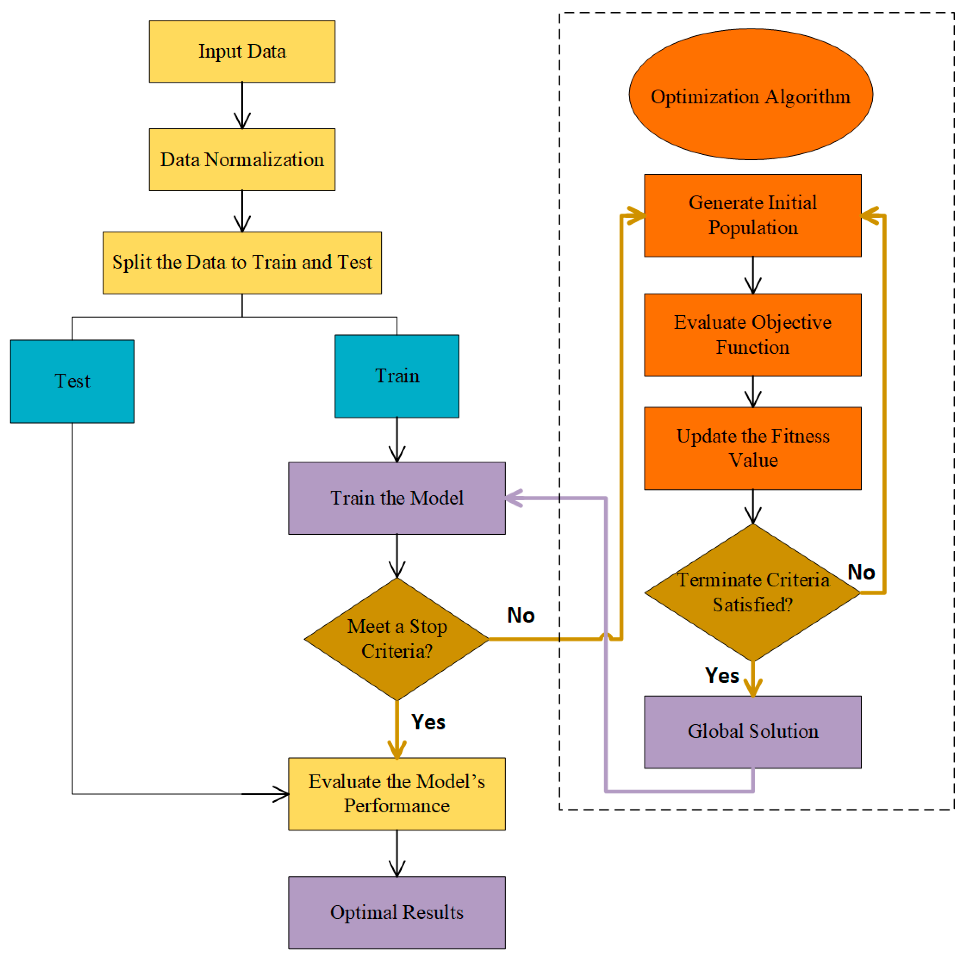
3.4.1. Combination of AI Models and Optimization Algorithms

A well-known category of hybrid models is based on combining AI models utilizing optimization algorithms inspired by biological processes, called bio-inspired (Figure 3). AI performance has been notably enhanced in diverse scenarios through the effective application of bio-inspired optimization algorithms [5,129,130,131,132,133,134]. Mohammadi and Mehdizadeh [135] demonstrated that using the whale optimization algorithm, as a bio-inspired algorithm, improved the AI’s accuracy in modeling daily ET₀ values. Other widely recognized bio-inspired algorithms, including genetic and firefly algorithms, have also shown significant improvements in the accuracy of AIs for modeling the evapotranspiration [136,137,138,139,140,141]. For instance, Maroufpoor et al. [142] investigated the capacity of the ANN-GWO, as a hybrid model, which is a combination of an ANN and grey wolf optimization algorithm, to approximate ET₀ in Iran under different climates. The ANN-GWO model’s efficiency was evaluated in comparison to the LSSVR and standalone ANN models. The results demonstrated a reduction in estimation errors by 42% and 30% when compared to the LS-SVR and ANN models, respectively. Among the different scenarios based on different input data combinations, the scenario that utilized only three inputs (i.e., wind speed and minimum and maximum temperature) demonstrated superiority over the other scenarios.

Wu et al. [143] assessed the performance of combining the ELM model with the flower pollination algorithm (FPA) and whale optimization algorithm (WOA) for monthly pan evaporation prediction. These models were further compared with ANN, improved M5Tree, and ELM optimized by differential evolution (DE), which is known as a floating-point evolutionary optimization algorithm. The climatic factors considered were wind speed, sunshine hours, relative humidity, and minimum and maximum temperatures. They noted that the hybrid ELM model demonstrated superior prediction accuracy against the hybrid M5Tree and ANN models. Additionally, the results explicitly indicate that the performance of the models is noticeably impacted by whether certain inputs are present or absent in the input sets. Among the five predictor variables examined, the maximum temperature and wind speed emerged as the two most effective predictors for accurately estimating ET₀. In the optimal ANN model, all five input variables were deemed significant in contrast to the other models. Additionally, across various performance indices, the ANN model outperformed the ELM and M5Tree models, despite the fact that their performances were generally comparable and closely aligned in most cases. The study carried out by Hadadi et al. [144] aimed to investigate the functionality of the ANFIS model along with its combinations with two optimization algorithms—specifically, the shuffled frog-leaping algorithm (SFLA) and GWO—in predicting monthly actual ET across the Neishaboor watershed located in Iran. The models’ input variables were categorized into three groups: (1) meteorological parameters, namely, air temperature (average, minimum, maximum), relative humidity, wind speed, sunshine hours, and dew point; (2) remotely sensed parameters, namely, net radiation, land surface temperature (LST), normalized difference vegetation index (NDVI), soil wetness deficit index (SWDI), and soil adjusted vegetation index (SAVI); and (3) hybrid predictors. The results indicated that the SWDI predictor had an indispensable effect on the estimation of ET in all three models. The estimation error was reduced by 12.5%, 17%, and 26.5% in the testing set and by 18.4%, 25.4%, and 24.5% in the training set in ANFIS, ANFIS-SFLA, and ANFIS-GWO, respectively. The findings also demonstrated the effectiveness of employing either optimization algorithm to enhance ET estimation. The most significant reduction in error rates in the testing set was observed for ANFIS-SFLA compared to ANFIS (12.5%), and ANFIS-GWO exhibited a decrease of 13.7% relative to ANFIS. Tang et al. [6] employed SVM and optimized ANN by a genetic algorithm (GA) to model actual ET in a partial plastic film mulching (MFR) and rainfed maize field under non-mulching (CK) conditions. Meteorological inputs, including minimum, mean, and maximum air temperature; minimum, mean, and maximum relative humidity; wind speed; and solar radiation; as well as crop input data such as plant height and LAI during the seasons in 2011–2012 when maize growing was employed to train the ANN-GA and SVM models. The results revealed that the GANN1 and SVM1 models, incorporating both meteorological and crop data as inputs, successfully predicted ET in maize. This confirmed the effectiveness of the GANN and SVM models in estimating ET in maize. Although the GANN2 and SVM2 models, which just used meteorological inputs, had comparatively lower efficiencies than the GANN1 and SVM1 models, their approximated outcomes remained satisfactory even when just meteorological data were accessible. Notably, the GANN models marginally outperformed the SVM models under both MFR and CK conditions, possibly because of the genetic algorithm optimization capability for ANN, which helps to avoid local minima and overfitting of the neural network.

Tikhamarine et al. [145] employed three different optimization algorithms, GA, GWO, and particle swarm optimizer (PSO), to enhance the precision of SVR in predicting the monthly ET₀ using wind speed, relative humidity, minimum and maximum air temperatures, and solar radiation at three sites in Algeria. The effectiveness of the proposed hybrid AI models was assessed in contrast to traditional ANNs and empirical models, including Ritchie, Turc, three variations of the Valiantzas, and Thornthwaite method. The results demonstrate that the hybrid models incorporating optimization algorithms exhibited superior performance compared to the standalone SVR models. Additionally, the SVR-GWO with five inputs, namely minimum and maximum temperature, wind speed, solar radiation, and relative humidity, exposed a feasible model to estimate ET₀. The GWO algorithm outperformed the GA and PSO algorithms. The conventional empirical methods employed in this study, excluding the Thornthwaite model, could demonstrate reliable estimates for ET₀. Furthermore, it is noteworthy to emphasize that the Valiantzas method performed better than other conventional approaches at the designated study stations.

Eslamian et al. [138] assessed the performance of ANN-GA and ANN models in modeling PM ET₀ using Esfahan, Iran’s province, meteorological data. The meteorological inputs included the average, minimum, and maximum air temperature, relative humidity, wind speed, and sunshine during a period from 1951 to 2005. The estimated values of the ANN-GA model outperformed the ANN model predictions when compared with a reference such as PM ET₀.

In a study conducted by Tikhamarine et al. [146], they put forward five hybrid models by combining ANN with five dissimilar optimization algorithms, namely GWO (ANN-GWO), PSO (ANN-PSO), multi-verse optimizer (ANN-MVO), ant lion optimizer (ANN-ALO), and WOA (ANN-WOA), to predict monthly ET₀ at two locations in Algeria and India. The predictions generated by these hybrid machine learning models were contrasted with those derived from the Valiantzas model. The comparative results indicated that the ANN-GWO-1 model was the most effective at both study stations, using five input variables (including maximum and minimum temperature, solar radiation, wind speed, and relative humidity).

The study carried out by Zounemat-Kermani et al. [147] aimed to evaluate the capabilities of three well-known ML approaches, that is, neural network autoregressive with exogenous input (NNARX), ANFIS, and GEP; five metaheuristic algorithms, that is, GA, PSO, firefly algorithm (FA), artificial bee colony (ABC), and continuous ant colony optimization (CACO); and two empirical relationships proposed through algebraic formulas for predicting the pan evaporation on a monthly basis at two meteorological stations. To achieve this goal, solar radiation, measured air temperature, wind speed, and relative humidity data were employed as inputs for the model. A comparison of the total evaporation estimates from the NNARX, GEP, and ANFIS models revealed that the ANFIS and NNARX predictions were closer to the measured one than those of the GEP model. The PSO algorithm performed the best among the five applied metaheuristic algorithms in predicting pan evaporation.

Kişi [148] evaluated the application of ENN in the modeling of pan evaporation on a monthly basis by employing inputs obtained from two stations in the Mediterranean Region of Turkey, including air temperature, pan evaporation, solar radiation, wind speed, and relative humidity. The ENNs used in this study were acquired using the adjustment of the ANN model’s weights by employing DE. The performance of ENN models was evaluated against ANFIS, FG, ANN, and SS models, revealing superior results in comparison to the alternatives. Additionally, the results indicated that the proposed models with inputs including full meteorological data outperformed the other models.

Ahmadi et al. [5] employed standalone GEP and SVR models as well as a proposed hybrid model by combining the intelligent water drop (IWD) and SVR algorithms considering different scenarios based on climatic inputs and historical ET₀ data to estimate monthly ET₀. The IWD algorithm acts as a meta-heuristic in order to optimize the weights among the layers of the model and the variables of the membership functions in SVR. The input weather data included the monthly minimum, mean, and maximum air temperature, relative humidity, sunshine duration, and wind speed at 2 m height. The findings indicated that in scenarios based on historical ET₀ data, the GEP models exhibited a slightly better performance against the SVR models. However, the best ET₀ estimates across all study sites were achieved using the hybrid SVR-IWD model.

Recent studies (e.g., Mehdizadeh et al. [135]) have explored the effectiveness of bio-inspired optimization algorithms to improve the accuracy of AI models for estimating ET₀ and pan evaporation. Bio-inspired algorithms like GA and firefly algorithms have also been used to optimize AI models, resulting in better predictions (e.g., Maroufpoor et al. [142]). In addition to these advancements, studies have combined ML models like ELM and SVM with optimization algorithms such as FPA and WOA [143]. Additionally, several studies have shown that incorporating a combination of meteorological and crop-related inputs, along with optimization algorithms, leads to more reliable predictions (e.g., Tang et al. [6] and Tikhamarine et al. [146]). These findings highlight the growing trend of using hybrid AI models and optimization algorithms to enhance the accuracy of ET estimations across diverse regions and climatic conditions.

3.4.2. Gene Expression Programming (GEP)

In accordance with the research conducted, employing function discovery techniques such as symbolic regression (SR) offers several advantages over other data-driven methods. SR, a nonlinear regression technique, aims to uncover suitable mathematical structures and algebraic expressions capable of capturing the nonlinearity problem tailored to the input data. Unlike traditional regression methods that require the user to predefine the model structure, SR automatically generates structures and formulates optimal algebraic expressions [149,150]. Furthermore, SR produces a generalized equation set that enables predictions across a significant spatial range, surpassing the capabilities of black-box data-driven methods [151]. SR primarily involves gene expression programming (GEP), which combines GA and genetic programming (GP). GEP, initially proposed by Ferreira [143], utilizes linear and simple chromosomes with consistent length, resembling the structure of a GA. In addition, it incorporates diverse branch structures along with varying sizes and configurations, comparable to the parsing trees utilized in GP, to construct its structure. Various research endeavors have investigated the predictive precision of GEP for estimating ET₀ [42,152,153,154]. For instance, Shiri et al. [155] employed the GEP model to predict daily ET₀ in Basque, Spain. They used daily meteorological data gathered from four weather stations, including solar radiation, wind speed, relative humidity, and air temperature, for the period—1999–2003—to estimate the PM ET₀. The efficiency of the GEP model was compared to that of models based on the Priestley–Taylor, ANFIS, and Hargreaves–Samani methods. The results demonstrated that the ANFIS and GEP models performed similarly, but the straightforward mathematical formulation in the GEP model positioned it as the favored option for estimating ET₀ in cases where the required meteorological data for the PM equation were not accessible. [156] conducted a study in Burkina Faso, where they employed GEP for estimating decadal ET₀ at four weather stations. They created a set of 16 distinct GEP models by employing various input parameters, including minimum, mean, and maximum air temperatures, sunshine hours, wind speed, relative humidity, and extra-terrestrial radiation. The findings highlight the reliability of GEP for ET₀ estimation because of its ability to present numerical models.

Wang Sheng et al. [157] employed GEP and ANN models to predict daily ET₀ at four stations in China’s southwestern Guangxi Province, known as the karst region. They developed 15 ANN and GEP models utilizing variables such as sunshine duration, maximum and minimum air temperatures, relative humidity, extra-terrestrial radiation, and wind speed. The study indicated that in general, ANN models displayed superior performance compared to their corresponding GEP counterparts. Moreover, the scenarios in which all inputs were considered in both ANN and GEP models were recognized as the most precise in the studied areas. Mehdizadeh et al. [116] carried out research in Iran, estimating the mean ET₀ on a monthly basis at 44 stations using GEP, SVM, MARS, and empirical equations. Sixteen different scenarios were proposed using monthly climate inputs, including the minimum, mean, and maximum temperature, wind speed at 2 m height, relative humidity, solar radiation, vapor pressure deficit, net, and extra-terrestrial radiation. The results showed that the AI methods outperformed the empirical equations, with the MARS model outperforming the GEP and SVM models.

Yassin et al. [158] employed GEP and ANN to determine daily ET₀ in the arid climate of Saudi Arabia using climatic data on minimum, mean, and maximum air temperature and relative humidity, solar radiation, wind speed, and reference crop height. They reported that ANN, with R² ranging from 67.6% to 99.8% and RMSE varying from 0.20 to 2.95 mm/day, slightly outperformed the GEP model in ET₀ estimation.

Gavili et al. [159] assessed the effectiveness of three soft computing approaches (GEP, ANFIS, and ANN) to model ET₀ using daily meteorological inputs including minimum and maximum temperature, sunshine hours, wind speed, and relative humidity. In addition to AI models, they used several empirical equations, such as Priestley–Taylor, Hargreaves−Samani, Hargreaves, Makkink, and Makkink−Hansen, and found that the AI models, as the leading approach in which the ANN is on top, outperformed the empirical methods.

The research highlights the advantages of SR over traditional data-driven methods, particularly in its ability to automatically generate optimal mathematical structures for nonlinear problems without requiring predefined models. SR, especially through GEP, combines genetic algorithms and programming to produce predictive models. Studies have demonstrated GEP’s effectiveness in estimating ET₀ across various regions and climates, such as Spain, Burkina Faso, China, and Saudi Arabia, comparing it to other models like ANFIS, ANN, and empirical equations. While GEP models often performed comparably or better than other methods, artificial intelligence-based models like ANN were sometimes found to outperform GEP in prediction accuracy, depending on the input variables and scenarios. These findings emphasize the reliability and versatility of GEP for ET₀ estimation, especially when meteorological data are limited.

3.4.3. Adaptive Neuro-Fuzzy Inference Systems (ANFIS)

ANFIS represents another significant subset of hybrid models that blend ANN with FG. These models translate the input parameters into output objectives using a combination of membership functions and conditional rules. Despite the ability of ANFIS to forecast changes in target variables with minimal input parameters and reasonable prediction precision, the enduring adaptability of neural networks is curtailed due to the arbitrary structure of the FG rules. In addition, incorporating further preprocessing entails time-consuming calculations in both frequency domains and time. Nonetheless, ANFIS remains a widely used choice for modeling evapotranspiration. Kişi and Öztürk [160] obtained ET₀ values using the PM equation with four years of climate parameter records on a daily basis and compared the results with empirical methods, ANN, and ANFIS, such as Hargreaves and Ritchie. The comparative analysis demonstrated that ANFIS, with inputs of relative humidity, radiation, temperature, and wind speed, outperformed ANN and empirical methods in modeling daily ET₀.

Dogan [161] investigated the performance of the ANFIS model in daily estimation of ET₀. Four ANFIS models were proposed by employing solar radiation, air temperature, wind speed, and relative humidity as the inputs collected at the Morgan Hill weather station in San Francisco, USA. The results demonstrated the successful implementation of the ANFIS model for estimating daily ET₀. In addition, the scenario incorporating all the input parameters exhibited the best performance.

Dou and Yang [16] utilized four different ML methods, namely ANFIS, ELM, ANN, and SVM, for estimating ET₀ in four different regions. The input data included air temperature, soil temperature, relative humidity, and net radiation. The results demonstrated that all models performed well in modeling daily ET, with high values for R² (ranged from 0.9398 to 0.9593) and NSE (ranged from 0.8877 to 0.9147) in the forest ecosystem. In the case of ANFIS, fuzzy c-means clustering and the subtractive clustering algorithms generally outperformed the grid-partitioning algorithm. The hybrid ELM methods, namely, complex ELM, online sequential ELM, and self-adaptive evolutionary ELM, among the ELM models, consistently performed better than the original ELM method across the studied sites, and the computational time required for training these models was significantly decreased. It shows that the advanced ANFIS and ELM models are valuable complements to the SVM and ANN methods because of their robustness and flexibility. Additionally, notable differences in modeling performance were observed between the four major ecosystem types. In forested areas, the models consistently demonstrated superior performance, whereas the lowest performance was observed in cropland ecosystems.

Kişi [162] examined the capabilities of ANN, ANFIS, and the SS models in predicting daily evaporation using different climatic inputs, including daily air temperature, pressure, wind speed, humidity, and solar radiation. Both approaches outperformed the conventional SS method with higher accuracy.

Moghaddamnia et al. [163] employed ANFIS and ANN models to simulate pan evaporation in different areas of Iran. The recorded meteorological data included daily wind speed, air temperature, saturation vapor, pan evaporation, relative humidity, and pressure deficit. Both ANN and ANFIS models demonstrated high capability in estimating pan evaporation values compared to empirical formulas, including Hefner, Lincare, and Marciano. However, ANN slightly outperformed the ANFIS.

del Cerro et al. [164] made a comparison between ANFIS and empirical equations, which are based on radiation and temperature, to model the daily ET₀ in southern India. The results indicated that the ANFIS model trained using meteorological data of temperature, solar radiation, relative humidity, and wind speed provided the most accurate estimates, with a root mean square difference (RMSD) of 0.002 and a correlation coefficient (R) of 0.999. Among the empirical models, the Ritchie method was identified as the most suitable for the region, yielding an RMSD of 0.507 and an R-value of 0.851. Furthermore, a sensitivity analysis was implemented to assess the stability of the best models when introducing errors in the inputs, which indicated the superiority of the empirical models over the ANFIS models.

Pour-Ali Baba et al. [165] investigated the performance of the ANFIS and ANN models in estimating daily ET₀ in Gwangju and Haenam, South Korea. Varied scenarios using sunshine hours, air temperature, relative humidity, and wind speed were considered for both ANN and ANFIS models. The results demonstrated that both the ANN and ANFIS models exhibited capability in the estimation of ET₀, surpassing the accuracy of the empirical equations, including the Priestly–Taylor, Hargreaves– Samani, and PM models.

Citakoglu et al. [166] predicted the mean ET₀ on a monthly basis using ANFIS and ANN models in Turkey at 275 stations based on different scenarios utilizing input parameters including relative humidity, air temperature, wind speed, and solar radiation. It was concluded that the scenario with all inputs yielded the highest accuracy. Additionally, the efficiency of the ANN and ANFIS models was investigated against two empirical equations of Hargreaves and Ritchie, with both models demonstrating higher accuracy than the empirical equations. Notably, the ANFIS model demonstrated a marginally superior performance compared to the ANN model.

Petković et al. [167] investigated the performance of the ANFIS model for estimating ET₀ on a monthly basis at twelve stations in Serbia. They defined 35 different patterns using variables such as minimum and maximum air temperatures, relative humidity, actual vapor pressure, sunshine hours, and wind speed. The results demonstrated that it is possible to estimate monthly ET₀ accurately using the ANFIS model by employing meteorological inputs, with sunshine hours being the most influential factor.

Cobaner [168] compared the performance of two types of ANFIS models, that is, ANFIS with subtractive clustering (ANFIS-SC) and grid partitioning (ANFIS-GP), in estimating ET₀ using daily weather data such as air temperature, solar radiation, wind speed, and relative humidity. In addition, these FIS models were investigated against the MLP and empirical models such as the CIMIS Penman, Ritchie, and Hargreaves methods. The results indicated that ANFIS-SC outperformed ANFIS-GP and other models with fewer computations.

Sanikhani et al. [169] assessed the prediction accuracy of the MLP, GRNN, RBFNN, ANFIS-GP, GEP, ANFIS-SC, Hargreaves–Samani, and calibrated Hargreaves–Samani models by employing monthly data from two stations in Turkey (i.e., Antalya and Isparta). The focus of this study was modeling ET₀ based on the temperature. The climate variables used to predict ET included solar radiation, minimum and maximum air temperatures, relative humidity, and wind speed monthly data over a 25-year period. The ranking of the AI models based on their prediction performance, measured by the RMSE and MAE, was as follows: RBFNN, ANFIS-SC, ANFIS-GP, MLP, GEP, GRNN, calibrated Hargreaves–Samani, and Hargreaves–Samani.

Zakhrouf et al. [170] evaluated the capability of ANFIS-SC, MLR, and ANFIS based on the fuzzy C-means clustering (ANFIS-F) in estimating daily ET₀ by climate data inputs of relative humidity, wind speed, insolation duration, and air temperature on a daily scale. The results revealed that the ANFIS-SC model considerably outperformed the MLR and ANFIS-F models.

The dynamic evolving neural fuzzy inference system (DENFIS) is also a hybrid computational model that employs the elements of NN and FG to create a system that can adapt and evolve over time to handle changing data patterns. The DENFIS is designed to provide accurate predictions in dynamic and non-linear environments. Ref. [171] employed two advanced ML algorithms, namely MARS and DENFIS, for estimating ET₀ on a daily scale by employing daily minimum and maximum temperatures. The hyperparameters of the models were optimized by applying two advanced metaheuristic optimization algorithms, bat Algorithm (BA) and WOA, resulting in four models: MARS-BA, MARS-WOA, DENFIS-BA, and DENFIS-WOA. These optimization algorithms have shown high efficiency in fine-tuning ML-based prediction models for problems in hydrological engineering [18,135,172,173,174,175]. By comparing the performances of the two AI-based optimization algorithms employed in this study, it was found that the WOA outperformed the BA. Superior performance of the WOA to evade entrapment in local optima may have participated in the enhanced effectiveness of the DENFIS model since its internal parameters were optimized by employing the WOA. In addition, DENFIS has the capacity to enhance its learning by dynamically developing the neuro-fuzzy functions of inputs and outputs and continuously updating the process of learning. This characteristic likely enables DENFIS to more reliably simulate ET in an environment with complex settings.

Malik et al. [176] assessed the suitability of the co-active neuro-fuzzy inference system (CANFIS) for predicting monthly ET₀ at two locations in India using meteorological data on a monthly basis, including wind speed, minimum and maximum air temperatures, solar radiation, and relative humidity. The effectiveness of the CANFIS models was investigated against that of the MLP, MLR, and RBFNN self-organizing map neural network (SOMNN) models. They concluded that CANFIS provided superior results compared with the other AI techniques used in this study.

Malik et al. [177] applied ANN MLR and CANFIS models to predict daily pan evaporation by employing different combinations of meteorological inputs such as relative humidity, minimum and maximum air temperature, sunshine hours, and wind speed in India at different stations. The findings revealed that the ANN models achieved higher success rates than other models.

In another study, Aytek [178] used CANFIS for daily ET₀ prediction using atmospheric parameters, including solar radiation, relative humidity, air temperature, and wind speed in California. The results indicated that the proposed model provided higher accuracy than the conventional Hargreaves and Turc equations.

This study [179] focused on the capability of three AI models, i.e., ANN, ANFIS, and ANN-gray wolf optimization (ANN-GWO), in estimating ET₀ in arid climates. These models were assessed with various input combinations, including minimum and maximum temperatures, ET₀, and wind speed. In data-scarce conditions, AI modes outperformed the Hargreaves equation, with ANFIS representing the most superior performance.

A substantial body of research has demonstrated the effectiveness of ANFIS and other ML models, as discussed above, in estimating ET₀ using meteorological inputs. Numerous studies have consistently shown that ANFIS models outperform traditional empirical methods, particularly when key climatic variables such as air temperature, wind speed, relative humidity, and solar radiation are incorporated [160,163,167]. In efforts to further enhance prediction accuracy, several studies have integrated ANFIS with clustering techniques and optimization algorithms (e.g., Ye et al. [171]). Advanced configurations, such as ANFIS-SC, have also shown improved performance compared to empirical models like the Hargreaves–Samani method, particularly across varying climatic regions [169,176]. These findings highlight some advantages of ANFIS over traditional empirical approaches in ET estimation.

ANFIS is particularly adept at modeling the intricate and nonlinear interactions among meteorological variables influencing ET, which are often oversimplified in empirical methods. Its data-driven architecture allows it to adaptively learn from patterns in the input data, enabling better handling of uncertainties and environmental variability [180,181]. Moreover, ANFIS supports hybridization with various metaheuristic optimization algorithms (e.g., Snake Optimizer), which further enhances its predictive capacity. This level of adaptability is lacking in empirical models, which are not designed for dynamic optimization based on dataset characteristics [180]. The application of ANFIS across a range of climatic conditions and datasets has also demonstrated its reliability and consistency, in contrast to empirical approaches that often require regional recalibration due to limited flexibility in response to changing climatic inputs [170,181].

A review of the literature allows for a comprehensive understanding of key methodological aspects such as data selection, preprocessing, feature selection, and the treatment of missing data in the context of ET₀ estimation using ANFIS models. ANFIS has demonstrated the capacity to accurately estimate ET₀ even with a limited set of climatic inputs, emphasizing its adaptability in utilizing alternative variables when conventional meteorological data are incomplete or unavailable [182]. Although the evaluation of acceptable error thresholds often relies on subjective criteria, hybrid adaptive neuro-fuzzy inference systems integrated with heuristic optimization algorithms have shown promise in addressing missing data challenges [183,184]. These hybrid approaches illustrate the potential of soft computing methods to deliver reliable ET₀ estimates across diverse environmental conditions and data availability constraints.

ANFIS represents a robust and effective approach for estimating ET, particularly in contexts characterized by incomplete meteorological data or the need to utilize non-traditional input variables. Its strength lies in its adaptability and flexibility; however, the model’s performance is highly contingent upon the quality, relevance, and adequacy of the input data. Despite its potential, the successful application of ANFIS often necessitates considerable domain expertise and computational resources to ensure optimal model configuration and performance.

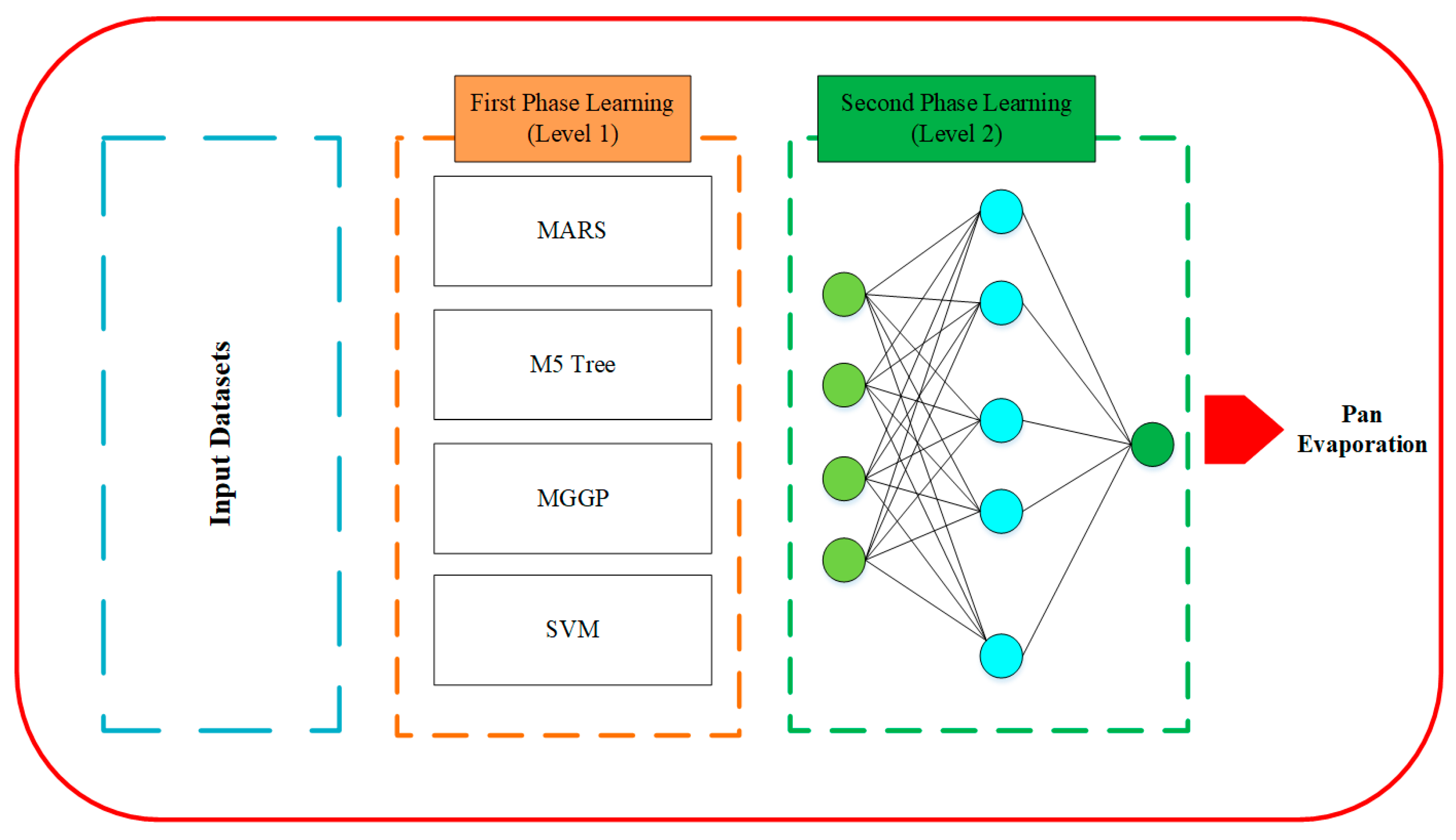
3.4.4. Combination of Different Models

Another type of hybridization is based on combining different algorithms with AI models, such as wavelet coupled with ANN [185,186], wavelet enhanced extreme learning machine [187], and wavelet transform regression model [188], to increase the estimation precision of evapotranspiration. Falamarzi et al. [185] employed wavelet-ANN (WNN) and ANN for predicting evapotranspiration on a daily scale from wind speed and temperature data. The results revealed that both models provided precise predictions for evapotranspiration.

Partal et al. [187] explored the feasibility of the wavelet extreme learning machine (WELM) model that combines discrete wavelet transform with ELM methods, in order to estimate ET₀ on a daily basis in Ankara and Kirikkale, Turkey. Different combinations of climatic inputs such as temperature, wind speed, solar radiation, and relative humidity were employed to train the models. The performance of the WELM model was investigated against the WANN, single ANN, ELM, and OS ELM models. The findings indicated that models incorporating all four inputs had higher precision than models with fewer input variables. Solar radiation was identified as the most influential input for the ET₀ estimation. Among the models tested, the WELM model emerged as the most accurate for estimating the ET₀. In addition, wavelet-based ensemble models, such as WELM and WANN, exhibit superior accuracy compared with single models.

Mehdizadeh et al. [189] employed GEP and MARS for estimating ET₀ on a daily basis in Iran. This study focused on six different climate stations in Iran, namely Urmia, Isfahan, Tabriz, Shiraz, Zahedan, and Yazd, representing semi-arid, arid, and hyper-arid climates, respectively. Daily weather data, including solar radiation, mean air temperature, wind speed at a height of 2 m, relative humidity, and ET₀ data, were utilized from 2000 to 2014 for this analysis. Two types of scenarios were considered as input: one dependent on weather data and the other on lagged ET₀ data. The findings of the local analysis revealed that both the GEP and MARS approaches were capable of estimating daily ET₀ using meteorological inputs and lagged ET₀ data. However, MARS exhibited the best performance under weather-data-based scenarios. Moreover, there were no significant differences in the models’ accuracy by employing data-based scenarios and lagged ET₀. In this study, novel hybrid models in lagged ET₀ data-based scenarios were proposed by combining GEP and MARS models with an autoregressive conditional heteroscedasticity (ARCH) time series model. The findings indicated that these hybrid models, namely GEP-ARCH and MARS-ARCH, promoted the effectiveness of modeling the ET₀ compared with using single GEP or MARS models at all studied stations. Furthermore, an external evaluation of the models’ performance at stations exhibiting comparable climatic conditions indicated that data from nearby stations could be applied in order to predict ET₀ on a daily basis at the target station. This finding suggests the potential applicability of neighboring station data for ET₀ estimation in similar climatic regions. According to the sensitivity analysis results, mean air temperature was found to be the best predictor for the accurate estimation of daily ET₀, while wind speed was identified to be the least influential predictor.

In order to optimize irrigation demands and improve crop resilience against water stress, Rahman, Hasan [190] combined AI models, including FFANN, CNN, GRU, and LSTM, with climatic data to predict ET, potential ET (PET), and CWSI in Bangladesh. To depict a wide range of possible future climate scenarios, the study used high-resolution climate data retrieved from ACCESS-ESM. Their findings indicated that the FFNN model, enhanced with a deep learning algorithm (FFNN-DLA), provided the most accurate predictions for representing spatio-temporal distributions of variables in different seasons.

Various statistical and ML models have been developed for ET₀ prediction; however, no single algorithm has proven universally optimal across all conditions. To address this, the current study [191] introduced a novel hybrid modeling approach, a combination of linear mixed effects (LME) model, nonlinear autoregressive neural network (NANN), and support vector machine (SVM) models to predict ET_0. NANN and SVM models are appropriate for capturing nonlinear residuals, while LME is capable of detecting linear patterns. Although both hybrid approaches performed well, the LME-SVM hybrid model demonstrated a slight advantage over the LME-NANN model. A summary of the studies conducted for estimating ET by employing hybrid models is presented in

Table 5. Studies conducted to model ET using hybrid techniques.

Reference	Models	Hybrid Model Type	Input	Output	Performance Criteria	Best Model(s)
Maroufpoor et al. [142]	ANN-GWO, LSSVR, ANN	Combination of AI models with optimization algorithms	Maximum and minimum temperatures, relative humidity, wind speed, sunshine hours, and precipitation	Monthly ET0	ScI = 0.077–0.187, R2 = 0.890–0.981, MAE = 0.279–0.717 mm/day	ANN-GWO
Wu et al. [143]	ELM-FPA, ELM-WOA, ANN, M5Tree, ELM-DE	Combination of AI models with optimization algorithms	Sunshine hours, wind speed, relative humidity, and maximum and minimum temperature	Monthly pan evaporation	R2 = 0.853–0.958, NSE = 0.766–0.956, RMSE = 0.2584–0.5032 mm/day, MAE = 0.2041–0.3726 mm/day, MAPE = 0.0928–0.1605	Hybrid ELM
Hadadi et al. [144]	ANFIS, ANFIS-SFLA, ANFIS-GWO	Combination of AI models with optimization algorithms	Meteorological data, including wind speed, relative humidity, air temperature (average, minimum, maximum), dew point, and sunshine hours, remotely sensed data, namely net radiation, NDVI, LST, SAVI, and SWDI	Actual ET	RMSE = 11.06, NSE = 0.74, RRMSE = 0.37	ANFIS-SFLA
Tang et al. [6]	SVM, ANN-GA	Combination of AI models with optimization algorithms	Meteorological data, including minimum, maximum, and mean air temperature; minimum, maximum, and mean relative humidity; solar radiation; and wind speed, as well as crop data like LAI and plant height	Daily actual ET	RMSE = 0.215–0.536 mm/day, MAE = 0.182–0.435 mm/day, NSE = 0.868–0.979	ANN-GA
Tikhamarine et al. [145]	SVR-GWO, SVR-GA, SVR-PSO, ANN, Turc, Ritchie, Thornthwaite, Valiantzas	Combination of AI models with optimization algorithms	Relative humidity, maximum and minimum air temperatures, solar radiation, and wind speed	Monthly ET0	RMSE = 0.0374–0.0776 mm, NSE = 0.9953–0.9995, PCC  =  0.9978–0.9998, WI  =  0.9988–0.9999	SVR-GWO
Eslamian et al. [138]	ANN, ANN-GA	Combination of AI models with optimization algorithms	Maximum, minimum, and average air temperature, relative humidity, wind speed, and sunshine duration	ET0	R2 = 0.9685, NMSE = 0.0675, MAE = 0.4751, MSE = 0.3693	ANN-GA
Tikhamarine et al. [146]	ANN-GWO, ANN-MVO, ANN-PSO, ANN-WOA, ANN-ALO, Valiantzas	Combination of AI models with optimization algorithms	Minimum and maximum air temperatures relative humidity, wind speed, solar radiation	Monthly ET0	RMSE = 0.0592–0.0808, NSE = 0.9956–0.9972, PCC = 0.9978–0.9986, WI = 0.9989–0.9993	ANN-GWO trained with minimum temperature, maximum temperature, relative humidity, wind speed, and solar radiation
Zounemat-Kermani et al. [147]	NNARX, GEP, and ANFIS models optimized by GA, PSO, CACO, ABC, and FA	Combination of AI models with optimization algorithms	Air temperature, solar radiation, relative humidity, and wind speed	Monthly pan evaporation	R2 = 0.959, RMSE = 0.631 mm, MAE = 0.447 mm, Kruskal–Wallis test = 0.0014	ANFIS-PSO
Kişi [148]	Priestley–Taylor, ANFIS, Hargreaves–Samani	Combination of AI models with optimization algorithms	Air temperature, relative humidity, wind speed, and solar radiation	Daily ET0	MAE = 0.603–1.345 mm, RMSE = 0.789–1.528 mm, R2 = 0.852–0.935	GEP
Ahmadi et al. [5]	SVR-IWD, GEP	Combination of AI models with optimization algorithms	Solar radiation, relative humidity, air temperature, wind speed, and pan evaporation	Monthly pan evaporation	RMSE = 0.210–1.064 mm/day, R = 0.838–0.996, MAE = 0.160–0.901 mm/day	SVR-IWD
Shiri et al. [155]	GEP	Combination of AI models with optimization algorithms	Minimum air temperature, maximum air temperature, mean air temperature, wind speed at 2 m height, sunshine duration, and relative humidity	Monthly ET0	RMSE = 0.316–1.159 mm/day, R2 = 0.881–0.967	GEP
Traore and Guven [156]	GEP, PM	Combination of GP and GA	Minimum, maximum, and mean air temperatures, relative humidity, extraterrestrial radiation, wind speed, and sunshine duration	Decadal ET0	RMSE = 0.108, R2 = 0.979	GEP
Wang Sheng et al. [157]	GEP, ANN	Combination of GP and GA	Minimum and maximum air temperatures, extraterrestrial radiation, relative humidity, wind speed, and sunshine duration	Daily ET0	R2 = 0.799–0.977, RMSE = 0.225–0.754 mm/day	GEP
Mehdizadeh et al. [116]	GEP, MARS, SVM, and empirical equations	Combination of GP and GA	Minimum temperature, maximum temperature, mean temperature, wind speed at 2 m height, relative humidity, solar radiation. vapor pressure deficit, extraterrestrial radiation, and net radiation	Monthly ET0	RMSE 0.07–1.75, MAE = 0.05–1.47, R2 = 0.331–0.999	MARS
Yassin et al. [158]	GEP and ANN	Combination of GP and GA	Air temperature (maximum, minimum, and mean), relative humidity (maximum, minimum, and mean), solar radiation, wind speed, and reference crop height	Daily ET0	R2 = 64.4–95.5%, RMSE = 1.13–3.1 mm/day	ANN
Gavili et al. [159]	ANN, ANFIS, GEP, Priestley−Taylor, Hargreaves−Samani, Hargreaves, Makkink, and Makkink−Hansen	Combination of GP and GA	Maximum temperature, minimum temperature, relative humidity, wind speed, and sunshine hours	Daily ET0	R2 = 0.9814–0.9873, RMSE = 0.3077–0.3451 mm, MAE = 0.2258–0.2483, NSE = 0.9812–0.9872	ANN
Kişi and Öztürk [160]	ANFIS, ANN, Hargreaves, Ritchie	Combination of NN and FG	Temperature, wind speed, relative humidity, and radiation	Daily ET0	R2 = 0.811–0.871, MSE = 0.615–0.712 mm2day2, MAE = 0.590–0.850 mm/day	ANFIS
Dogan [161]	ANFIS, PM	Combination of NN and FG	Air temperature, solar radiation, relative humidity, and wind speed	Daily ET0	AARE = 6.4%, R2 = 0.996, MSE = 0.016	ANFIS
Dou and Yang [16]	ANFIS, ELM, ANN, SVM	Combination of NN and FG	Air temperature, soil temperature, net radiation, and relative humidity	Daily ET0	R2 = 0.9398–0.9593, NSE = 0.8817–0.9147, RMSE = 0.3138–0.6807, MAE = 0.2217–0.4821	Advanced ANFIS and ELM models
Kişi [162]	ANFIS, ANN, SS	Combination of NN and FG	Air temperature, solar radiation, humidity, pressure, wind speed	Daily pan evaporation	MSE = 0.09–6.23 mm2/day2, MARE = 3.40–17.9%, R2 = 0.860–0.998	ANFIS
Moghaddamnia et al. [163]	ANFIS, ANN	Combination of NN and FG	Air temperature, wind speed, saturation vapor pressure deficit, relative humidity, and pan evaporation	Daily pan evaporation	RMSE = 1.51–2.47%, R2 = 0.92–0.97	ANN, ANFIS
del Cerro et al. [164]	ANFIS, PM, Ritchie, Irmak, Blaney–Criddle, Priestley–Taylor, Hargreaves, Baier–Robertson, McGuiness–Bordne, Jensen–Haise, Turc, Modified Turc, Makkink	Combination of NN and FG	Solar radiation, temperature, wind speed, and relative humidity	Daily ET0	d = 0.6415–0.9999, MAE = 0.0008–0.7746, SEE = 0.0016–0.5534, RMSD = 0.0016–1.0197	ANFIS, Ritchie
Pour-Ali Baba et al. [165]	ANFIS, ANN, Hargreaves–Samani, Priestly–Taylor, PM	Combination of NN and FG	Air temperature, sunshine hours, wind speed, and relative humidity	Daily ET0	RMSE = 0.474–0.965 mm, MAE = 0.307–0.659 mm, NSE = 0.764–0.959, R2 = 0.765–0.959	ANFIS, ANN
Citakoglu et al. [166]	ANFIS, ANN, Hargreaves, Ritchie	Combination of NN and FG	Air temperature, relative humidity, solar radiation, and wind speed	Monthly ET0	RMSE = 0.198–0.486, MAE = 0.345–0.538, R2 = 0.960–0.985	ANFIS
Petković et al. [167]	ANFIS	Combination of NN and FG	Maximum and minimum air temperatures, maximum and minimum relative humidity, wind speed, actual vapor pressure, and sunshine hours	Monthly ET0	RMSE = 0.3148 mm/day, R = 0.9801, R2 = 0.9607	ANFIS trained by minimum temperature, maximum humidity, and actual vapor pressure
Cobaner [168]	ANFIS-GP, ANFIS-SC, MLP, CIMIS Penman, Hargreaves, Ritchie	Combination of NN and FG	Solar radiation, air temperature, relative humidity, and wind speed	Daily ET0	RMSE = 0.11–0.66 mm, MAE = 0.06–1.12 mm, R2 = 0.507–0.995	ANFIS-SC
Sanikhani et al. [169]	MLP, GRNN, RBFNN, ANFIS-GP, ANFIS-SC, GEP, Hargreaves–Samani, and calibrated Hargreaves–Samani	Combination of NN and FG	Solar radiation, minimum and maximum air temperatures, relative humidity, and wind speed	Daily ET0	RMSE = 0.524 mm/day, MAE = 0.383, R2 = 0.905	RBNN
Zakhrouf et al. [170]	ANFIS-SC, ANFIS-F, MLR	Combination of NN and FG	Relative humidity, insolation duration, wind speed, and air temperature	Daily ET0	MARE = 16.43%, MSE = 0.316 mm2, ME = 0.30 mm, NSE = 94.01%	ANFIS-SC
Ye et al. [171]	DENFIS-WOA, DENFIS-BA, MARS-WOA, and MARS-BA	Combination of NN and FG	Maximum and minimum temperature, ET0	Daily ET0	NRMSE = 0.35–0.54, SD = 1.00–1.01, R2 = 0.85–0.94, md = 0.73–0.82, NSE = 0.71–0.87, KGE = 0.70–0.86	DENFIS-WOA
Malik et al. [176]	CANFIS, MLP, RBFNN, SOMNN, MLR	Combination of NN and FG	Minimum and maximum air temperatures, wind speed, relative humidity, and solar radiation	Monthly ET0	RMSE = 0.0978–0.1394, ScI = 0.0261–0.0475, CE = 0.9846–0.9963, PCC = 0.9942–0.9982, WI = 0.9959–0.9991	CANFIS
Malik et al. [177]	CANFIS, MLR, ANN	Combination of NN and FG	Relative humidity, air temperature (maximum and minimum), wind speed, and sunshine hours	Daily pan evaporation	RMSE = 1.233–1.406 mm/day, CE = 0.729–0.792, R = 0.887–0.921	ANN
Aytek [178]	CANFIS, Hargreaves, Turc	Combination of NN and FG	Solar radiation, relative humidity, air temperature, and wind speed	Daily ET0	RMSE = 0.13 mm/day, CE = 0.97%, R2 = 0.98	CANFIS
Falamarzi et al. [185]	ANN, WNN	Combination of different models	Temperature and wind speed	Daily ET0	R = 0.82–0.90, RMSE = 1.10–1.54 mm/day, APE = 23–30%, NSE = 0.53–0.76	ANN, WNN
Kişi [187]	WELM, ANN, ELM, and OS-ELM	Combination of different models	Temperature, solar radiation, relative humidity, and wind speed	Daily ET0	RMSE 0.3590–1.6381 mm/day, R2 = 0.0.2617–0.9518, MAE = 0.3848–1.3774 mm/day, NSE = 0.2334–0.9492	WELM
Mehdizadeh [189]	MARS-ARCH and GEP-ARCH	Combination of different models	Air temperature, solar radiation, relative humidity, wind speed, ET0	Daily ET0	RMSE = 0.40–1.85 mm/day, R2 = 0.200–0.962, MAE = 0.29–1.64 mm/day, MAPE = 11.20–105.50%	MARS-ARCH and GEP-ARCH
Rahman et al. [190]	FFNN, CNN, GRU, and LSTM	Combination of different models	Air temperature, humidity, solar radiation, wind speed, maximum and minimum temperature, and precipitation	Daily ET and PET	R2 = 0.94	FFNN-DLA
Bidabadi et al. [179]	ANN, ANFIS, and ANN-GWO	Combination of NN with FG and optimization algorithms	Minimum and maximum air temperature, wind speed, and ET0	Monthly ET0	RMSE = 0.335–0.434, R2 = 0.947–0.970, MSE = 0.112–0.212	ANFIS
Habeeb et al. [191]	LME-SVM, LME-NANN	Combination of different models	Wind speed, maximum and minimum temperatures, average temperature, humidity, and ET0	Monthly ET0	MAE = 5.0580–6.9283, MAPE = 1.8713–2.9077, RMSE = 6.1883–9.6620	LME-SVM

Notes: Abbreviations: peak percentage deviation (Pdv), average absolute relative error (AARE), root mean square difference (RMSD), mean error (ME), average performance error (APE), scatter index (ScI), modified index of agreement (md), performance indicator (GPI), uncertainty with a 95% confidence level (U95), linear mixed effects (LME), nonlinear autoregressive neural network (NANN), Pearson correlation coefficient (PCC), coefficient of efficiency (CE).

.

Recent investigations (e.g., [189,190,191]) have explored hybrid modeling approaches for ET₀ estimation, reporting consistent—albeit marginal—improvements in predictive performance over standalone models. These hybrid methods offer clear advantages over traditional empirical techniques, including enhanced accuracy, better adaptability to complex datasets, improved interpretability, robustness in data-scarce contexts, more refined estimation of ET components, and reduced uncertainty. Frameworks such as RF-XGBoost and XGBoost-LightGBM have reliably outperformed empirical models by achieving superior statistical metrics—higher KGE and R², and lower RMSE—thereby supporting more dependable ET estimates, especially under variable meteorological conditions [78].

Hybrid models demonstrate the capacity to process a wide range of meteorological variables—temperature, relative humidity, solar radiation, and wind speed—addressing a major limitation of empirical approaches and enabling application across diverse climates [78,192]. Models that integrate additive regression with decision tree-based algorithms or ensemble strategies (e.g., RF-M5Tree) strike a favorable balance between predictive accuracy and interpretability. Moreover, their compatibility with remote sensing data and physically based simulations enhances their utility in regions with limited ground-based observations. These capabilities position hybrid models as a significant advancement in ET estimation methodologies, enabling accurate prediction across heterogeneous climatic settings [78,81,193].

A key strength of hybrid models is their ability to integrate multi-source datasets, which helps mitigate issues stemming from sparse observational networks. This often involves combining conventional meteorological data (e.g., air temperature, humidity, wind speed) with remote sensing inputs such as satellite-derived vegetation indices and outputs from eddy covariance systems or physically based models [81,194]. Ensuring computational efficiency and predictive reliability typically requires steps like data normalization and hyperparameter tuning, particularly in models such as XGBoost [78]. Feature selection also plays a crucial role in enhancing performance; in semi-arid regions, temperature-based inputs tend to offer more consistency and reliability than solar radiation variables [78,195]. XGBoost-based hybrids have shown strong performance using combinations of minimum and maximum temperature, solar radiation, humidity, and wind speed [78], reinforcing their adaptability to variable climate conditions and data availability constraints.

Research has underscored the utility of models like RF-XGBoost, which combine high accuracy with moderate interpretability [78]. Deep learning-based hybrids, such as deep long short-term memory (D-LSTM) models, have demonstrated promising results even in data-scarce environments, although often at the expense of transparency and interpretability [196]. Despite their strengths, hybrid models face notable limitations. Equifinality—where multiple parameter sets yield similar outputs—can introduce uncertainty and diminish reliability [197]. These challenges highlight the need for continued refinement to ensure model robustness, particularly when applied across differing climatic regimes or regions.

Hybrid models often integrate metaheuristic optimizers (PSO, GA, Grey Wolf, etc.) to tune parameters, yielding notably better generalization [198]. Modern hybrids not only improve raw predictive accuracy but can also reveal dominant physical drivers: e.g., GEP models in multi-climate tests identified mean relative humidity as the key determinant of ET₀ variability [199]. By combining algorithms (ANN, fuzzy systems, tree ensembles, etc.) with evolutionary optimization, current hybrids provide expressive, flexible models that learn complex ET₀ relationships beyond what classic empirical formulas or simple ML can capture.

On the other hand, one of the challenges is model complexity and computational cost. Advanced hybrids (ensembles of deep nets or many tree models) can require heavy training resources. In one comparative study, RF ensembles gave the best ET₀ estimates but suffered much greater computation than simpler models [200]. Overfitting is another concern: data-driven hybrids like GEP or ANFIS can fit training data too closely, especially with limited records. Ensuring the transferability of a hybrid model to new regions or climate regimes remains an open issue. Recent reviews recommend attention to domain-adaptation strategies (e.g., transfer learning or multi-site training) to improve robustness, since many ML-based ET₀ models fail when relocated.

4. Comparison Between Time Series and AI Models

Comparing time-series and AI models, some studies have reported the advantage of time-series models compared to AI. For example, Aghelpour et al. [201] utilized a hybrid model called ANFIS-DE, a combination of ANFIS and DE, as well as seasonal autoregressive integrated moving average (SARIMA), a classic stochastic time series model, for monthly ET forecasting using input weather data, including air temperature, sunshine duration, and relative humidity. The findings demonstrated the ability of the DE algorithm to significantly promote the accuracy of the simple ANFIS model. However, SARIMA was considered the most suitable model compared to ANFIS and ANFIS-DE for ET₀ predictions on a monthly basis in all study areas. Ashrafzadeh et al. [202] used SVM, GMDH, and SARIMA models to predict ET₀ in Guilan Province, Iran. It was found that the models could predict ET₀ for the subsequent two years; nevertheless, the SARIMA models generally showed better performance than the SVM and GMDH models. Aghelpour et al. [203] compared several stochastic models, such as autoregressive, moving average, autoregressive moving average, and autoregressive integrated moving average (ARIMA), with three AI models (SVM, GRNN, and ANFIS) for daily ET₀ prediction. Although both model types demonstrated high capability in the prediction of daily ET₀ rates for humid regions, the time series models were preferred over AI models, similar to the studies conducted by Ashrafzadeh et al. [202,204], which suggested that linear autocorrelation is more robust compared to nonlinear autocorrelation in the ET₀ time series, explaining the preference for time series models in the study conducted by Aghelpour et al. [201] because of their higher accuracy and ease of use. It should be noted that the limitations of the SARIMA model, which only considers time lags of the evaporation variable as inputs, led to the application of machine learning models using ET₀ time lags to enable a meaningful comparison. Additionally, in Tamil Nadu, India, ref. [205] compared AI and stochastic methods and concluded that stochastic models were more suitable for ET₀ prediction. Conversely, in a study conducted in Brazil [206], AI models provided relatively more accurate predictions of ET₀ compared to time series models, which contradicts the findings of the aforementioned studies. They compared the CNN model with the SARIMA stochastic model for daily ET prediction using meteorological data. This discrepancy could be due to the differences in climatic conditions between the study areas. Landeras et al. [207] conducted a comparison between stochastic and AI methods, that is, ARIMA and ANN, for predicting weekly ET in Spain using meteorological data, including air temperature, relative humidity, wind speed, and solar radiation. According to the results, both types of models improved the weekly ET₀ predictions compared to the mean-based models; however, the AI model slightly outperformed the stochastic model.

5. Challenges to AI Models

Despite the increasing application of AI techniques in estimating ET₀, the use of black-box models without incorporating the fundamental physical principles underlying the ET process can lead to significant inaccuracies [208]. A critical challenge in deploying AI models for ET₀ prediction lies in the quality and quantity of the training data. Small or noisy datasets may prevent these models from learning the true underlying patterns. Specifically, limited data can result in overfitting, where the model captures noise rather than meaningful trends, while excessively noisy data may cause underfitting, particularly when simple learning architectures are used [208]. To mitigate these issues, data preprocessing techniques such as normalization, bias reduction, and expansion of training datasets are essential. Another key consideration is the selection of relevant input features, as the choice of climatic parameters directly influences model accuracy. However, despite their importance, these preprocessing and feature selection methods have been underutilized in many AI-based ET modeling studies. For instance, Goyal et al. [106] evaluated multiple combinations of input variables, ranging from a full set including rainfall, temperature extremes, relative humidity, and sunshine hours to reduced sets with fewer variables—using the Gamma test (GT). Their results indicated that including all six climatic parameters yielded the highest accuracy in estimating pan evaporation. Similarly, other studies have employed GT to construct optimal input combinations by minimizing mean square error (MSE). One study [54] found that a combination of relative humidity, minimum and maximum temperatures, sunshine hours, and wind speed provided optimal performance for monthly pan evaporation prediction. Moghaddamnia et al. [163] used the Gamma test across various regions in Iran to assess the impact of input selection on evaporation simulation. While wind speed emerged as the most influential factor based on GT results, this contradicted intuitive assessments that identified air temperature as the most relevant. This inconsistency highlights the complexity and spatial variability in the influence of climatic parameters on ET processes. In another study, Ahmadi et al. [5] employed τ-Kendall and entropy-based methods to identify effective inputs from a dataset comprising minimum, mean, and maximum air temperature, wind speed at 2 m height, relative humidity, and sunshine duration. Their findings showed that models using climatic data outperformed those based solely on antecedent ET₀ values. Air temperature and solar radiation were consistently significant, while wind speed also played a notable role, especially in the τ-Kendall method.

The contribution of wind speed to ET₀ estimation has been further validated in prior research. Although wind speed alone may result in poor model performance, its inclusion alongside other climatic inputs substantially improves estimation accuracy [116,166]. Nevertheless, a persistent challenge in AI-based ET modeling is the variability in optimal input combinations across studies. For example, Wen et al. [114] found that SVM performed well using only minimum and maximum temperatures and solar radiation, while Antonopoulos et al. [32] identified temperature, relative humidity, and wind speed as the best predictors for ANN. Such inconsistencies restrict the generalizability of AI models and underscore the need for location-specific and model-specific input selection strategies.

In addition to the limitations mentioned above, emerging challenges in AI-based ET₀ estimation relate to model generalizability across diverse climatic and geographic regions, the dynamic and nonlinear behavior of environmental variables, and the inadequate temporal adaptability inherent in many existing predictive frameworks. AI models that are predominantly trained on static historical datasets often exhibit poor performance when exposed to non-stationary climate conditions, which are increasingly prevalent due to the compounded effects of global climate change, anthropogenic land-use transformations, and shifting agricultural practices. These evolving conditions introduce variability that traditional machine learning models are not inherently designed to accommodate. Furthermore, the reliance on region-specific datasets for training restricts the spatial transferability of models, as they may fail to capture the localized hydrometeorological characteristics of distinct agroecological or hydrological regimes. Without rigorous retraining, recalibration, or the use of domain adaptation strategies, the applicability of these models across broader regions remains limited [209,210,211].

6. Conclusions and Future Studies

ET is the combined process of water vapor transfer to the atmosphere through evaporation from surfaces and transpiration from plants. Accurate ET estimation is vital for agriculture, water resource management, climate studies, and ecological assessments. The choice of estimation methods depends on data availability, computational resources, and required accuracy. ET estimation approaches are broadly classified into direct and indirect methods. Direct methods, though accurate, are often limited by high costs, maintenance demands, and localized measurements. Indirect methods, particularly the Penman–Monteith (PM) model, are widely used but require extensive input data, which may not be available globally. As an alternative, AI techniques offer a promising solution due to their ability to model the nonlinear nature of ET processes. This study explores the use of AI in ET estimation—specifically ET₀, actual ET, and pan evaporation—using four model types: neuron-based, tree-based, kernel-based, and hybrid models.

ANN models that fall into the neuron-based category have gained popularity for estimating ET because of their capability to capture complex nonlinear relationships among input variables and output estimates. Although this type of method is well-suited for large datasets with intricate patterns and various data distributions, it suffers from overfitting under limited data conditions and is difficult to interpret, especially in the case of deep architecture. Similarly, tree-based models, especially deep trees, can overfit; however, ensemble methods, such as RF and GB, can mitigate overfitting and generalize effectively. Furthermore, tree-based models can handle non-linear relationships and missing datasets and are more interpretable than neural network-based models. Unlike the aforementioned methods, kernel-based methods are able to capture fewer non-linear relationships and are well-suited for small- to medium-sized datasets. Additionally, selecting an appropriate kernel function is challenging because it requires domain expertise. According to previous studies that estimated ET using AI models, ANNs have been extensively employed due to their flexibility and generalization ability. Another type of neuron-based model, that is, DNN, has rarely been used by researchers, while the superior performance of RNNs compared to simple ANNs is demonstrated in studies. This can be because of additional capabilities in their architecture, like the additional memory units to maintain historical data records. Likewise, CNN can extract valuable features for modeling tasks. The challenges related to data, resources, complexity, and interpretability likely contributed to their reduced use in ET modeling compared to traditional ANNs. Among tree-based models, RF and other ensemble methods have shown acceptable performance in ET modeling. In addition, many investigations concluded that hybrid models, including optimized AI models, ANFIS, GEP, and other combined models, outperformed traditional models due to integrating the strengths of various models to enhance predictive performance.

To further advance the applicability and robustness of AI-based ET prediction, future research should target several strategic areas. A particularly promising direction involves the application of transfer learning, where models initially trained in data-rich regions are adapted for data-scarce areas through fine-tuning or domain adaptation techniques. This not only reduces the reliance on extensive local datasets but also significantly enhances spatial generalizability, making it highly suitable for large-scale ET₀ mapping across diverse climatic zones. In addition, there is increasing recognition of the importance of integrating socioeconomic variables, such as land use change, irrigation intensity, and anthropogenic landscape transformations, into AI modeling frameworks. These factors play a pivotal role in shaping ET dynamics, particularly in rapidly transforming agricultural and peri-urban regions, and their inclusion can lead to more context-sensitive and policy-relevant predictions. Furthermore, the development of climate-adaptive AI frameworks offers a compelling path forward. By incorporating real-time climatic indices (e.g., ENSO events, drought severity indicators) into the model architecture, such systems can dynamically recalibrate in response to evolving environmental conditions. This adaptability is essential for enhancing model resilience under extreme climate variability and can provide critical decision support for sustainable water resource planning and agricultural management in an era of intensifying climate change.

In this regard, there are some concluding remarks outlining potential directions for future studies:

• The integration of physical ET processes into AI models to reduce inaccuracies from the current black-box approaches.
• The development of standardized input variable combinations for AI-based ET₀ estimation to address inconsistencies in variable selection across similar climate conditions.
• The exploration and implementation of advanced pre-processing techniques to improve input variable selection and overall model accuracy.
• A combination of AI models with hydrological modeling and remote sensing data for more accurate, real-time, or near-real-time ET estimations at various spatiotemporal scales.
• The establishment of benchmarks for consistent evaluation of ET₀ models across different geographic and climatic contexts by integrating domain-specific knowledge and multi-source data.
• The transfer learning enhances model generalizability by adapting knowledge from data-rich regions to data-scarce areas.
• Socioeconomic factors, including land use changes and irrigation practices, are crucial for context-sensitive ET₀ predictions.

References

1. Taheri, M.; Mohammadian, A.; Ganji, F.; Bigdeli, M.; Nasseri, M. Energy-based approaches in estimating actual evapotranspiration focusing on land surface temperature: A review of methods, concepts, and challenges. Energies 2022, 15, 1264. [Google Scholar] [CrossRef]
2. Omar, P.J.; Gupta, P.; Wang, Q. Exploring the rise of AI-based smart water management systems. AQUA Water Infrastruct. Ecosyst. Soc. 2023, 72, iii–iv. [Google Scholar] [CrossRef]
3. Abdullah, S.S.; Malek, M.A. Empirical Penman-Monteith equation and artificial intelligence techniques in predicting reference evapotranspiration: A review. Int. J. Water 2016, 10, 55–66. [Google Scholar] [CrossRef]
4. Granata, F. Evapotranspiration evaluation models based on machine learning algorithms—A comparative study. Agric. Water Manag. 2019, 217, 303–315. [Google Scholar] [CrossRef]
5. Ahmadi, F.; Mehdizadeh, S.; Mohammadi, B.; Pham, Q.B.; Doan, T.N.C.; Vo, N.D. Application of an artificial intelligence technique enhanced with intelligent water drops for monthly reference evapotranspiration estimation. Agric. Water Manag. 2021, 244, 106622. [Google Scholar] [CrossRef]
6. Tang, D.; Feng, Y.; Gong, D.; Hao, W.; Cui, N. Evaluation of artificial intelligence models for actual crop evapotranspiration modeling in mulched and non-mulched maize croplands. Comput. Electron. Agric. 2018, 152, 375–384. [Google Scholar] [CrossRef]
7. Allen, R.G.; Pereira, L.S.; Raes, D.; Smith, M. Crop Evapotranspiration-Guidelines for Computing Crop Water Requirements-FAO Irrigation and Drainage Paper 56; FAO: Rome, Italy, 1998; pp. 147–151. [Google Scholar]
8. Allen, R.G. Using the FAO-56 dual crop coefficient method over an irrigated region as part of an evapotranspiration intercomparison study. J. Hydrol. 2000, 229, 27–41. [Google Scholar] [CrossRef]
9. Ding, R.; Kang, S.; Zhang, Y.; Hao, X.; Tong, L.; Du, T. Partitioning evapotranspiration into soil evaporation and transpiration using a modified dual crop coefficient model in irrigated maize field with ground-mulching. Agric. Water Manag. 2013, 127, 85–96. [Google Scholar] [CrossRef]
10. Ferreira, L.B.; da Cunha, F.F.; de Oliveira, R.A.; Fernandes Filho, E.I. Estimation of reference evapotranspiration in Brazil with limited meteorological data using ANN and SVM–A new approach. J. Hydrol. 2019, 572, 556–570. [Google Scholar] [CrossRef]
11. Huang, G.; Wu, L.; Ma, X.; Zhang, W.; Fan, J.; Yu, X.; Zeng, W.; Zhou, H. Evaluation of CatBoost method for prediction of reference evapotranspiration in humid regions. J. Hydrol. 2019, 574, 1029–1041. [Google Scholar] [CrossRef]
12. Qutbudin, I.; Shiru, M.S.; Sharafati, A.; Ahmed, K.; Al-Ansari, N.; Yaseen, Z.M.; Shahid, S.; Wang, X. Seasonal drought pattern changes due to climate variability: Case study in Afghanistan. Water 2019, 11, 1096. [Google Scholar] [CrossRef]
13. dos Santos Farias, D.B.; Althoff, D.; Rodrigues, L.N.; Filgueiras, R. Performance evaluation of numerical and machine learning methods in estimating reference evapotranspiration in a Brazilian agricultural frontier. Theor. Appl. Climatol. 2020, 142, 1481–1492. [Google Scholar] [CrossRef]
14. Yang, Y.; Sun, H.; Xue, J.; Liu, Y.; Liu, L.; Yan, D.; Gui, D. Estimating evapotranspiration by coupling Bayesian model averaging methods with machine learning algorithms. Environ. Monit. Assess. 2021, 193, 156. [Google Scholar] [CrossRef] [PubMed]
15. Kumar, M.; Raghuwanshi, N.; Singh, R.; Wallender, W.; Pruitt, W. Estimating evapotranspiration using artificial neural network. J. Irrig. Drain. Eng. 2002, 128, 224–233. [Google Scholar] [CrossRef]
16. Dou, X.; Yang, Y. Evapotranspiration estimation using four different machine learning approaches in different terrestrial ecosystems. Comput. Electron. Agric. 2018, 148, 95–106. [Google Scholar] [CrossRef]
17. Ehteram, M.; Singh, V.P.; Ferdowsi, A.; Mousavi, S.F.; Farzin, S.; Karami, H.; Mohd, N.S.; Afan, H.A.; Lai, S.H.; Kisi, O.; et al. An improved model based on the support vector machine and cuckoo algorithm for simulating reference evapotranspiration. PLoS ONE 2019, 14, e0217499. [Google Scholar] [CrossRef]
18. Chia, M.Y.; Huang, Y.F.; Koo, C.H. Support vector machine enhanced empirical reference evapotranspiration estimation with limited meteorological parameters. Comput. Electron. Agric. 2020, 175, 105577. [Google Scholar] [CrossRef]
19. Penman, H.L. Natural evaporation from open water, bare soil and grass. Proc. R. Soc. London. Ser. A Math. Phys. Sci. 1948, 193, 120–145. [Google Scholar]
20. Monteith, J.L. Evaporation and environment. The stage and movement of water in living organisms. In 19th Symp. Society for Experimental Biology; Cambridge University Press: Cambridge, UK, 1965. [Google Scholar]
21. Wróblewski, P.; Drożdż, W.; Lewicki, W.; Miązek, P. Methodology for assessing the impact of aperiodic phenomena on the energy balance of propulsion engines in vehicle electromobility systems for given areas. Energies 2021, 14, 2314. [Google Scholar] [CrossRef]
22. Luo, X.; Chen, J.M.; Liu, J.; Black, T.A.; Croft, H.; Staebler, R.; He, L.; Arain, M.A.; Chen, B.; Mo, G.; et al. Comparison of big-leaf, two-big-leaf, and two-leaf upscaling schemes for evapotranspiration estimation using coupled carbon-water modeling. J. Geophys. Res. Biogeosci. 2018, 123, 207–225. [Google Scholar] [CrossRef]
23. Alves, I.; Perrier, A.; Pereira, L. Aerodynamic and surface resistances of complete cover crops: How good is the “big leaf”? In Transactions of the ASAE; ASABE: St Joseph, MI, USA, 1998; Volume 41, pp. 345–351. [Google Scholar]
24. Shuttleworth, W.J.; Wallace, J. Evaporation from sparse crops-an energy combination theory. Q. J. R. Meteorol. Soc. 1985, 111, 839–855. [Google Scholar] [CrossRef]
25. Zhao, W.; Li, A. A review on land surface processes modelling over complex terrain. Adv. Meteorol. 2015, 2015, 1–17. [Google Scholar] [CrossRef]
26. Skhiri, A.; Ferhi, A.; Bousselmi, A.; Khlifi, S.; Mattar, M.A. Artificial neural network for forecasting reference evapotranspiration in semi-arid bioclimatic regions. Water 2024, 16, 602. [Google Scholar] [CrossRef]
27. Kişi, Ö. Generalized regression neural networks for evapotranspiration modelling. Hydrol. Sci. J. 2006, 51, 1092–1105. [Google Scholar] [CrossRef]
28. Wang, X.; Li, W.; Li, Q. A new embedded estimation model for soil temperature prediction. Sci. Program. 2021, 2021, 1–16. [Google Scholar] [CrossRef]
29. Kisi, O. The potential of different ANN techniques in evapotranspiration modelling. Hydrol. Process. 2008, 22, 2449–2460. [Google Scholar] [CrossRef]
30. Landeras, G.; Ortiz-Barredo, A.; López, J.J. Comparison of artificial neural network models and empirical and semi-empirical equations for daily reference evapotranspiration estimation in the Basque Country (Northern Spain). Agric. Water Manag. 2008, 95, 553–565. [Google Scholar] [CrossRef]
31. El-Baroudy, I.; Elshorbagy, A.; Carey, S.; Giustolisi, O.; Savic, D. Comparison of three data-driven techniques in modelling the evapotranspiration process. J. Hydroinform. 2010, 12, 365–379. [Google Scholar] [CrossRef]
32. Antonopoulos, V.Z.; Antonopoulos, A.V. Daily reference evapotranspiration estimates by artificial neural networks technique and empirical equations using limited input climate variables. Comput. Electron. Agric. 2017, 132, 86–96. [Google Scholar] [CrossRef]
33. Kisi, O. Fuzzy genetic approach for modeling reference evapotranspiration. J. Irrig. Drain. Eng. 2010, 136, 175–183. [Google Scholar] [CrossRef]
34. Traore, S.; Wang, Y.-M.; Kerh, T. Artificial neural network for modeling reference evapotranspiration complex process in Sudano-Sahelian zone. Agric. Water Manag. 2010, 97, 707–714. [Google Scholar] [CrossRef]
35. Nema, M.K.; Khare, D.; Chandniha, S.K. Application of artificial intelligence to estimate the reference evapotranspiration in sub-humid Doon valley. Appl. Water Sci. 2017, 7, 3903–3910. [Google Scholar] [CrossRef]
36. Sudheer, K.; Gosain, A.; Ramasastri, K. Estimating actual evapotranspiration from limited climatic data using neural computing technique. J. Irrig. Drain. Eng. 2003, 129, 214–218. [Google Scholar] [CrossRef]
37. Bruton, J.; McClendon, R.; Hoogenboom, G. Estimating daily pan evaporation with artificial neural networks. In Transactions of the ASAE; ASABE: St Joseph, MI, USA, 2000; Volume 43, pp. 491–496. [Google Scholar]
38. Sudheer, K.; Gosain, A.; Mohana Rangan, D.; Saheb, S. Modelling evaporation using an artificial neural network algorithm. Hydrol. Process. 2002, 16, 3189–3202. [Google Scholar] [CrossRef]
39. Keskin, M.E.; Terzi, Ö. Artificial neural network models of daily pan evaporation. J. Hydrol. Eng. 2006, 11, 65–70. [Google Scholar] [CrossRef]
40. Aytek, A.; Guven, A.; Yuce, M.I.; Aksoy, H. An explicit neural network formulation for evapotranspiration. Hydrol. Sci. J. 2008, 53, 893–904. [Google Scholar] [CrossRef]
41. Rahimikhoob, A. Estimation of evapotranspiration based on only air temperature data using artificial neural networks for a subtropical climate in Iran. Theor. Appl. Climatol. 2010, 101, 83–91. [Google Scholar] [CrossRef]
42. Parasuraman, K.; Elshorbagy, A.; Carey, S.K. Modelling the dynamics of the evapotranspiration process using genetic programming. Hydrol. Sci. J. 2007, 52, 563–578. [Google Scholar] [CrossRef]
43. Tezel, G.; Buyukyildiz, M. Monthly evaporation forecasting using artificial neural networks and support vector machines. Theor. Appl. Climatol. 2016, 124, 69–80. [Google Scholar] [CrossRef]
44. Aghelpour, P.; Bahrami-Pichaghchi, H.; Karimpour, F. Estimating daily rice crop evapotranspiration in limited climatic data and utilizing the soft computing algorithms MLP, RBF, GRNN, and GMDH. Complexity 2022, 2022, 4534822. [Google Scholar] [CrossRef]
45. Kişi, Ö. Modeling monthly evaporation using two different neural computing techniques. Irrig. Sci. 2009, 27, 417–430. [Google Scholar] [CrossRef]
46. Traore, S.; Luo, Y.; Fipps, G. Deployment of artificial neural network for short-term forecasting of evapotranspiration using public weather forecast restricted messages. Agric. Water Manag. 2016, 163, 363–379. [Google Scholar] [CrossRef]
47. Trajkovic, S. Temperature-based approaches for estimating reference evapotranspiration. J. Irrig. Drain. Eng. 2005, 131, 316–323. [Google Scholar] [CrossRef]
48. Tabari, H.; Hosseinzadeh Talaee, P. Multilayer perceptron for reference evapotranspiration estimation in a semiarid region. Neural Comput. Appl. 2013, 23, 341–348. [Google Scholar] [CrossRef]
49. Zhu, B.; Feng, Y.; Gong, D.; Jiang, S.; Zhao, L.; Cui, N. Hybrid particle swarm optimization with extreme learning machine for daily reference evapotranspiration prediction from limited climatic data. Comput. Electron. Agric. 2020, 173, 105430. [Google Scholar] [CrossRef]
50. Feng, Y.; Jia, Y.; Cui, N.; Zhao, L.; Li, C.; Gong, D. Calibration of Hargreaves model for reference evapotranspiration estimation in Sichuan basin of southwest China. Agric. Water Manag. 2017, 181, 1–9. [Google Scholar] [CrossRef]
51. Patil, A.P.; Deka, P.C. An extreme learning machine approach for modeling evapotranspiration using extrinsic inputs. Comput. Electron. Agric. 2016, 121, 385–392. [Google Scholar] [CrossRef]
52. Heddam, S.; Kisi, O.; Sebbar, A.; Houichi, L.; Djemili, L. New formulation for predicting daily reference evapotranspiration (et 0) in the mediterranean region of Algeria country: Optimally pruned extreme learning machine (opelm) versus online sequential extreme learning machine (oselm). In Water Resources in Algeria-Part I: Assessment of Surface and Groundwater Resources; Springer Nature: Berlin/Heidelberg, Germany, 2020; pp. 181–199. [Google Scholar]
53. Malik, A.; Kumar, A.; Kisi, O. Daily pan evaporation estimation using heuristic methods with gamma test. J. Irrig. Drain. Eng. 2018, 144, 04018023. [Google Scholar] [CrossRef]
54. Malik, A.; Kumar, A.; Kim, S.; Kashani, M.H.; Karimi, V.; Sharafati, A.; Ghorbani, M.A.; Al-Ansari, N.; Salih, S.Q.; Yaseen, Z.M.; et al. Modeling monthly pan evaporation process over the Indian central Himalayas: Application of multiple learning artificial intelligence model. Eng. Appl. Comput. Fluid Mech. 2020, 14, 323–338. [Google Scholar] [CrossRef]
55. Makwana, J.J.; Tiwari, M.K.; Deora, B.S. Development and comparison of artificial intelligence models for estimating daily reference evapotranspiration from limited input variables. Smart Agric. Technol. 2023, 3, 100115. [Google Scholar] [CrossRef]
56. Güzel, H.; Üneş, F.; Erginer, M.; Kaya, Y.Z.; Taşar, B.; Erginer, İ.; Demirci, M. A Comparative Study on Daily Evapotranspiration Estimation by Using Various Artificial Intelligence Techniques and Traditional Regression Calculations; AIMS Press: Springfield, MO, USA, 2023. [Google Scholar]
57. Abdel-Fattah, M.K.; Kotb Abd-Elmabod, S.; Zhang, Z.; Merwad, A.R.M. Exploring the Applicability of Regression models and Artificial neural networks for calculating reference evapotranspiration in arid regions. Sustainability 2023, 15, 15494. [Google Scholar] [CrossRef]
58. Novotná, B.; Cviklovič, V.; Chvíla, B.; Minárik, M. Application of Developing Artificial Intelligence (AI) Techniques to Model Pan Evaporation Trends in Slovak River Sub-Basins. Sustainability 2025, 17, 526. [Google Scholar] [CrossRef]
59. Faloye, O.T.; Ajayi, A.E.; Babalola, T.; Omotehinse, A.O.; Adeyeri, O.E.; Adabembe, B.A.; Ogunrinde, A.T.; Okunola, A.; Fashina, A. Modelling crop evapotranspiration and water use efficiency of maize using artificial neural network and linear regression models in biochar and inorganic fertilizer-amended soil under varying water applications. Water 2023, 15, 2294. [Google Scholar] [CrossRef]
60. Eludire, O.O.; Faloye, O.T.; Alatise, M.; Ajayi, A.E.; Oguntunde, P.; Badmus, T.; Fashina, A.; Adeyeri, O.E.; Olorunfemi, I.E.; Ogunrinde, A.T. Evaluation of Evapotranspiration Prediction for Cassava Crop Using Artificial Neural Network Models and Empirical Models over Cross River Basin in Nigeria. Water 2025, 17, 87. [Google Scholar] [CrossRef]
61. Diamantopoulou, M.; Georgiou, P.; Papamichail, D. Performance evaluation of artificial neural networks in estimating reference evapotranspiration with minimal meteorological data. Glob. NEST J. 2011, 13, 18–27. [Google Scholar]
62. Genaidy, M. Estimating of evapotranspiration using artificial neural network. Misr J. Agric. Eng. 2020, 37, 81–94. [Google Scholar] [CrossRef]
63. Kartal, V. Prediction of monthly evapotranspiration by artificial neural network model development with Levenberg–Marquardt method in Elazig, Turkey. Environ. Sci. Pollut. Res. 2024, 31, 20953–20969. [Google Scholar] [CrossRef]
64. Dimitriadou, S.; Nikolakopoulos, K.G. Artificial neural networks for the prediction of the reference evapotranspiration of the Peloponnese Peninsula, Greece. Water 2022, 14, 2027. [Google Scholar] [CrossRef]
65. Sattari, M.T.; Apaydin, H.; Band, S.S.; Mosavi, A.; Prasad, R. Comparative analysis of kernel-based versus ANN and deep learning methods in monthly reference evapotranspiration estimation. Hydrol. Earth Syst. Sci. 2021, 25, 603–618. [Google Scholar] [CrossRef]
66. Shi, H.; Cai, X. Extrapolability improvement of machine learning-based evapotranspiration models via domain-adversarial neural networks. Environ. Model. Softw. 2025, 187, 106383. [Google Scholar] [CrossRef]
67. Hettiarachchi, P.; Hall, M.; Minns, A. The extrapolation of artificial neural networks for the modelling of rainfall—Runoff relationships. J. Hydroinform. 2005, 7, 291–296. [Google Scholar] [CrossRef]
68. Lipton, Z.C.; Berkowitz, J.; Elkan, C. A critical review of recurrent neural networks for sequence learning. arXiv 2015, arXiv:1506.00019. [Google Scholar]
69. Hochreiter, S.; Schmidhuber, J. Long short-term memory. Neural Comput. 1997, 9, 1735–1780. [Google Scholar] [CrossRef]
70. Afzaal, H.; Farooque, A.A.; Abbas, F.; Acharya, B.; Esau, T. Computation of evapotranspiration with artificial intelligence for precision water resource management. Appl. Sci. 2020, 10, 1621. [Google Scholar] [CrossRef]
71. Saggi, M.K.; Jain, S. Reference evapotranspiration estimation and modeling of the Punjab Northern India using deep learning. Comput. Electron. Agric. 2019, 156, 387–398. [Google Scholar] [CrossRef]
72. Farooque, A.A.; Afzaal, H.; Abbas, F.; Bos, M.; Maqsood, J.; Wang, X.; Hussain, N. Forecasting daily evapotranspiration using artificial neural networks for sustainable irrigation scheduling. Irrig. Sci. 2022, 40, 55–69. [Google Scholar] [CrossRef]
73. Fang, S.L.; Lin, Y.S.; Chang, S.C.; Chang, Y.L.; Tsai, B.Y.; Kuo, B.J. Using artificial intelligence algorithms to estimate and short-term forecast the daily reference evapotranspiration with limited meteorological variables. Agriculture 2024, 14, 510. [Google Scholar] [CrossRef]
74. Baishnab, U.; Hossen Sajib, M.S.; Islam, A.; Akter, S.; Hasan, A.; Roy, T.; Das, P. Deep learning approaches for short-crop reference evapotranspiration estimation: A case study in Southeastern Australia. Earth Sci. Inform. 2025, 18, 4. [Google Scholar] [CrossRef]
75. Ba-ichou, A.; Zegoumou, A.; Benhlima, S.; Bekr, M.A. Daily reference evapotranspiration estimation utilizing deep learning models with varied combinations of weather data. In Proceedings of the E3S Web of Conferences, 9–20 May 2023; EDP Sciences: Kenitra, Morocco; Volume 492, p. 01002. [Google Scholar]
76. Treder, W.; Klamkowski, K.; Wójcik, K.; Tryngiel-Gać, A. Evapotranspiration estimation using machine learning methods. J. Hortic. Res. 2023, 31, 35–44. [Google Scholar] [CrossRef]
77. Ravindran, S.M.; Bhaskaran, S.K.M.; Ambat, S.K.N. A deep neural network architecture to model reference evapotranspiration using a single input meteorological parameter. Environ. Process. 2021, 8, 1567–1599. [Google Scholar] [CrossRef]
78. Acharki, S.; Raza, A.; Vishwakarma, D.K.; Amharref, M.; Bernoussi, A.S.; Singh, S.K.; Al-Ansari, N.; Dewidar, A.Z.; Al-Othman, A.A.; Mattar, M.A. Comparative assessment of empirical and hybrid machine learning models for estimating daily reference evapotranspiration in sub-humid and semi-arid climates. Sci. Rep. 2025, 15, 2542. [Google Scholar] [CrossRef] [PubMed]
79. Kraft, B.; Nelson, J.A.; Walther, S.; Gans, F.; Weber, U.; Duveiller, G.; Reichstein, M.; Zhang, W.; Rußwurm, M.; Tuia, D.; et al. On the added value of sequential deep learning for upscaling evapotranspiration. EGUsphere 2024, 2024, 1–30. [Google Scholar]
80. Caminha, H.D.; da Silva, T.L.C.; da Rocha, A.R.; Lima, S.C.R.V. Estimating Reference Evapotranspiration using Data Mining Prediction Models and Feature Selection. In Proceedings of the ICEIS (1), Porto, Portugal, 26–29 April 2017; pp. 272–279. [Google Scholar]
81. Chen, J.; Dafflon, B.; Tran, A.P.; Falco, N.; Hubbard, S.S. A deep learning hybrid predictive modeling (HPM) approach for estimating evapotranspiration and ecosystem respiration. Hydrol. Earth Syst. Sci. 2021, 25, 6041–6066. [Google Scholar] [CrossRef]
82. Farhangmehr, V.; Imanian, H.; Mohammadian, A.; Cobo, J.H.; Shirkhani, H.; Payeur, P. A spatiotemporal CNN-LSTM deep learning model for predicting soil temperature in diverse large-scale regional climates. Sci. Total Environ. 2025, 968, 178901. [Google Scholar] [CrossRef]
83. Im, M.S.; Dasari, V.R. Computational complexity reduction of deep neural networks. arXiv 2022, arXiv:2207.14620. [Google Scholar]
84. Karimi, S.; Shiri, J.; Marti, P. Supplanting missing climatic inputs in classical and random forest models for estimating reference evapotranspiration in humid coastal areas of Iran. Comput. Electron. Agric. 2020, 176, 105633. [Google Scholar] [CrossRef]
85. Shiri, J. Improving the performance of the mass transfer-based reference evapotranspiration estimation approaches through a coupled wavelet-random forest methodology. J. Hydrol. 2018, 561, 737–750. [Google Scholar] [CrossRef]
86. Wang, S.; Lian, J.; Peng, Y.; Hu, B.; Chen, H. Generalized reference evapotranspiration models with limited climatic data based on random forest and gene expression programming in Guangxi, China. Agric. Water Manag. 2019, 221, 220–230. [Google Scholar] [CrossRef]
87. Gonzalo-Martin, C.; Lillo-Saavedra, M.; Garcia-Pedrero, A.; Lagos, O.; Menasalvas, E. Daily evapotranspiration mapping using regression random forest models. IEEE J. Sel. Top. Appl. Earth Obs. Remote Sens. 2017, 10, 5359–5368. [Google Scholar] [CrossRef]
88. Shi, L.; Feng, P.; Wang, B.; Li Liu, D.; Cleverly, J.; Fang, Q.; Yu, Q. Projecting potential evapotranspiration change and quantifying its uncertainty under future climate scenarios: A case study in southeastern Australia. J. Hydrol. 2020, 584, 124756. [Google Scholar] [CrossRef]
89. Vulova, S.; Meier, F.; Rocha, A.D.; Quanz, J.; Nouri, H.; Kleinschmit, B. Modeling urban evapotranspiration using remote sensing, flux footprints, and artificial intelligence. Sci. Total Environ. 2021, 786, 147293. [Google Scholar] [CrossRef] [PubMed]
90. Feng, Y.; Cui, N.; Gong, D.; Zhang, Q.; Zhao, L. Evaluation of random forests and generalized regression neural networks for daily reference evapotranspiration modelling. Agric. Water Manag. 2017, 193, 163–173. [Google Scholar] [CrossRef]
91. Al-Mukhtar, M. Modeling the monthly pan evaporation rates using artificial intelligence methods: A case study in Iraq. Environ. Earth Sci. 2021, 80, 39. [Google Scholar] [CrossRef]
92. Hameed, M.M.; AlOmar, M.K.; Mohd Razali, S.F.; Kareem Khalaf, M.A.; Baniya, W.J.; Sharafati, A.; AlSaadi, M.A. Application of artificial intelligence models for evapotranspiration prediction along the southern coast of Turkey. Complexity 2021, 2021, 1–20. [Google Scholar] [CrossRef]
93. Fan, J.; Ma, X.; Wu, L.; Zhang, F.; Yu, X.; Zeng, W. Light Gradient Boosting Machine: An efficient soft computing model for estimating daily reference evapotranspiration with local and external meteorological data. Agric. Water Manag. 2019, 225, 105758. [Google Scholar] [CrossRef]
94. Wu, L.; Fan, J. Comparison of neuron-based, kernel-based, tree-based and curve-based machine learning models for predicting daily reference evapotranspiration. PLoS ONE 2019, 14, e0217520. [Google Scholar] [CrossRef]
95. Keshtegar, B.; Piri, J.; Kisi, O. A nonlinear mathematical modeling of daily pan evaporation based on conjugate gradient method. Comput. Electron. Agric. 2016, 127, 120–130. [Google Scholar] [CrossRef]
96. Wang, L.; Kisi, O.; Zounemat-Kermani, M.; Li, H. Pan evaporation modeling using six different heuristic computing methods in different climates of China. J. Hydrol. 2017, 544, 407–427. [Google Scholar] [CrossRef]
97. Katimbo, A.; Rudnick, D.R.; Zhang, J.; Ge, Y.; DeJonge, K.C.; Franz, T.E.; Shi, Y.; Liang, W.-z.; Qiao, X.; Heeren, D.M.; et al. Evaluation of artificial intelligence algorithms with sensor data assimilation in estimating crop evapotranspiration and crop water stress index for irrigation water management. Smart Agric. Technol. 2023, 4, 100176. [Google Scholar] [CrossRef]
98. Sun, D.; Zhang, H.; Qi, Y.; Ren, Y.; Zhang, Z.; Li, X.; Lv, Y.; Cheng, M. A Comparative Analysis of Different Algorithms for Estimating Evapotranspiration with Limited Observation Variables: A Case Study in Beijing, China. Remote Sens. 2025, 17, 636. [Google Scholar] [CrossRef]
99. Garofalo, S.P.; Ardito, F.; Sanitate, N.; De Carolis, G.; Ruggieri, S.; Giannico, V.; Rana, G.; Ferrara, R.M. Robustness of Actual Evapotranspiration Predicted by Random Forest Model Integrating Remote Sensing and Meteorological Information: Case of Watermelon (Citrullus lanatus,(Thunb) Matsum. & Nakai, 1916). Water 2025, 17, 323. [Google Scholar] [CrossRef]
100. Abed, M.; Imteaz, M.A.; Ahmed, A.N.; Huang, Y.F. Modelling monthly pan evaporation utilising Random Forest and deep learning algorithms. Sci. Rep. 2022, 12, 13132. [Google Scholar] [CrossRef] [PubMed]
101. Wu, M.; Feng, Q.; Wen, X.; Deo, R.C.; Yin, Z.; Yang, L.; Sheng, D. Random forest predictive model development with uncertainty analysis capability for the estimation of evapotranspiration in an arid oasis region. Hydrol. Res. 2020, 51, 648–665. [Google Scholar] [CrossRef]
102. Rai, P.; Kumar, P.; Al-Ansari, N.; Malik, A. Evaluation of machine learning versus empirical models for monthly reference evapotranspiration estimation in Uttar Pradesh and Uttarakhand States, India. Sustainability 2022, 14, 5771. [Google Scholar] [CrossRef]
103. Ayaz, A.; Rajesh, M.; Singh, S.K.; Rehana, S. Estimation of reference evapotranspiration using machine learning models with limited data. AIMS Geosci. 2021, 7, 268–290. [Google Scholar] [CrossRef]
104. Amani, S.; Shafizadeh-Moghadam, H. A review of machine learning models and influential factors for estimating evapotranspiration using remote sensing and ground-based data. Agric. Water Manag. 2023, 284, 108324. [Google Scholar] [CrossRef]
105. Shrestha, N.; Shukla, S. Support vector machine based modeling of evapotranspiration using hydro-climatic variables in a sub-tropical environment. Agric. For. Meteorol. 2015, 200, 172–184. [Google Scholar] [CrossRef]
106. Kisi, O. Modeling reference evapotranspiration using three different heuristic regression approaches. Agric. Water Manag. 2016, 169, 162–172. [Google Scholar] [CrossRef]
107. Goyal, M.K.; Bharti, B.; Quilty, J.; Adamowski, J.; Pandey, A. Modeling of daily pan evaporation in sub tropical climates using ANN, LS-SVR, Fuzzy Logic, and ANFIS. Expert Syst. Appl. 2014, 41, 5267–5276. [Google Scholar] [CrossRef]
108. Cherkassky, V.; Krasnopolsky, V.; Solomatine, D.P.; Valdes, J. Computational intelligence in earth sciences and environmental applications: Issues and challenges. Neural Netw. 2006, 19, 113–121. [Google Scholar] [CrossRef]
109. Elshorbagy ACorzo, G.; Srinivasulu, S.; Solomatine, D.P. Experimental Investigation of the Predictive Capabilities of Data Driven Modeling Techniques in Hydrology-Part 1: Concepts and methodology. Hydrol. Earth Syst. Sci. 2010, 14, 1931–1941. [Google Scholar] [CrossRef]
110. Jain, S.; Nayak, P.; Sudheer, K. Models for estimating evapotranspiration using artificial neural networks, and their physical interpretation. Hydrol. Process. Int. J. 2008, 22, 2225–2234. [Google Scholar] [CrossRef]
111. Abdullah, S.S.; Malek, M.A.; Abdullah, N.S.; Kisi, O.; Yap, K.S. Extreme learning machines: A new approach for prediction of reference evapotranspiration. J. Hydrol. 2015, 527, 184–195. [Google Scholar] [CrossRef]
112. Güçlü, Y.S.; Subyani, A.M.; Şen, Z. Regional fuzzy chain model for evapotranspiration estimation. J. Hydrol. 2017, 544, 233–241. [Google Scholar] [CrossRef]
113. Yu, H.; Wen, X.; Li, B.; Yang, Z.; Wu, M.; Ma, Y. Uncertainty analysis of artificial intelligence modeling daily reference evapotranspiration in the northwest end of China. Comput. Electron. Agric. 2020, 176, 105653. [Google Scholar] [CrossRef]
114. Tabari, H.; Kisi, O.; Ezani, A.; Talaee, P.H. SVM, ANFIS, regression and climate based models for reference evapotranspiration modeling using limited climatic data in a semi-arid highland environment. J. Hydrol. 2012, 444, 78–89. [Google Scholar] [CrossRef]
115. Wen, X.; Si, J.; He, Z.; Wu, J.; Shao, H.; Yu, H. Support-vector-machine-based models for modeling daily reference evapotranspiration with limited climatic data in extreme arid regions. Water Resour. Manag. 2015, 29, 3195–3209. [Google Scholar] [CrossRef]
116. Sobh, M.T.; Nashwan, M.S.; Amer, N. High-resolution reference evapotranspiration for arid Egypt: Comparative analysis and evaluation of empirical and artificial intelligence models. Int. J. Climatol. 2022, 42, 10217–10237. [Google Scholar] [CrossRef]
117. Mehdizadeh, S.; Behmanesh, J.; Khalili, K. Using MARS, SVM, GEP and empirical equations for estimation of monthly mean reference evapotranspiration. Comput. Electron. Agric. 2017, 139, 103–114. [Google Scholar] [CrossRef]
118. Adnan, R.M.; Heddam, S.; Yaseen, Z.M.; Shahid, S.; Kisi, O.; Li, B. Prediction of potential evapotranspiration using temperature-based heuristic approaches. Sustainability 2020, 13, 297. [Google Scholar] [CrossRef]
119. Muhammad Adnan, R.; Chen, Z.; Yuan, X.; Kisi, O.; El-Shafie, A.; Kuriqi, A.; Ikram, M. Reference evapotranspiration modeling using new heuristic methods. Entropy 2020, 22, 547. [Google Scholar] [CrossRef] [PubMed]
120. Kisi, O. Pan evaporation modeling using least square support vector machine, multivariate adaptive regression splines and M5 model tree. J. Hydrol. 2015, 528, 312–320. [Google Scholar] [CrossRef]
121. Eslamian, S.; Abedi-Koupai, J.; Amiri, M.; Gohari, S. Estimation of Daily Reference Evapotranspiration Using Support Vector. Res. J. Environ. Sci. 2009, 3, 439–447. [Google Scholar]
122. Nourani, V.; Elkiran, G.; Abdullahi, J. Multi-station artificial intelligence based ensemble modeling of reference evapotranspiration using pan evaporation measurements. J. Hydrol. 2019, 577, 123958. [Google Scholar] [CrossRef]
123. Wang, L.; Niu, Z.; Kisi, O.; Yu, D. Pan evaporation modeling using four different heuristic approaches. Comput. Electron. Agric. 2017, 140, 203–213. [Google Scholar] [CrossRef]
124. Allawi, M.F.; Jaafar, O.; Hamzah, F.M.; El-Shafie, A. Novel reservoir system simulation procedure for gap minimization between water supply and demand. J. Clean. Prod. 2019, 206, 928–943. [Google Scholar] [CrossRef]
125. Deo, R.C.; Samui, P.; Kim, D. Estimation of monthly evaporative loss using relevance vector machine, extreme learning machine and multivariate adaptive regression spline models. Stoch. Environ. Res. Risk Assess. 2016, 30, 1769–1784. [Google Scholar] [CrossRef]
126. Torres, A.F.; Walker, W.R.; McKee, M. Forecasting daily potential evapotranspiration using machine learning and limited climatic data. Agric. Water Manag. 2011, 98, 553–562. [Google Scholar] [CrossRef]
127. Tausif, M.; Iqbal, M.W.; Bashir, R.N.; AlGhofaily, B.; Elyassih, A.; Khan, A.R. Federated learning based reference evapotranspiration estimation for distributed crop fields. PLoS ONE 2025, 20, e0314921. [Google Scholar] [CrossRef]
128. Chia, M.Y.; Huang, Y.F.; Koo, C.H.; Fung, K.F. Recent advances in evapotranspiration estimation using artificial intelligence approaches with a focus on hybridization techniques—A review. Agronomy 2020, 10, 101. [Google Scholar] [CrossRef]
129. Ahmadianfar, I.; Shirvani-Hosseini, S.; He, J.; Samadi-Koucheksaraee, A.; Yaseen, Z.M. An improved adaptive neuro fuzzy inference system model using conjoined metaheuristic algorithms for electrical conductivity prediction. Sci. Rep. 2022, 12, 4934. [Google Scholar] [CrossRef] [PubMed]
130. Mehdizadeh, S.; Mohammadi, B.; Ahmadi, F. Establishing coupled models for estimating daily dew point temperature using nature-inspired optimization algorithms. Hydrology 2022, 9, 9. [Google Scholar] [CrossRef]
131. Babanezhad, M.; Behroyan, I.; Nakhjiri, A.T.; Marjani, A.; Rezakazemi, M.; Heydarinasab, A.; Shirazian, S. Investigation on performance of particle swarm optimization (PSO) algorithm based fuzzy inference system (PSOFIS) in a combination of CFD modeling for prediction of fluid flow. Sci. Rep. 2021, 11, 1505. [Google Scholar] [CrossRef]
132. Mohammadi, B.; Guan, Y.; Moazenzadeh, R.; Safari, M.J.S. Implementation of hybrid particle swarm optimization-differential evolution algorithms coupled with multi-layer perceptron for suspended sediment load estimation. Catena 2021, 198, 105024. [Google Scholar] [CrossRef]
133. Aghelpour, P.; Varshavian, V. Forecasting different types of droughts simultaneously using multivariate standardized precipitation index (MSPI), MLP neural network, and imperialistic competitive algorithm (ICA). Complexity 2021, 2021, 1–16. [Google Scholar] [CrossRef]
134. Deo, R.C.; Ghorbani, M.A.; Samadianfard, S.; Maraseni, T.; Bilgili, M.; Biazar, M. Multi-layer perceptron hybrid model integrated with the firefly optimizer algorithm for windspeed prediction of target site using a limited set of neighboring reference station data. Renew. Energy 2018, 116, 309–323. [Google Scholar] [CrossRef]
135. Mohammadi, B.; Mehdizadeh, S. Modeling daily reference evapotranspiration via a novel approach based on support vector regression coupled with whale optimization algorithm. Agric. Water Manag. 2020, 237, 106145. [Google Scholar] [CrossRef]
136. Roy, D.K.; Lal, A.; Sarker, K.K.; Saha, K.K.; Datta, B. Optimization algorithms as training approaches for prediction of reference evapotranspiration using adaptive neuro fuzzy inference system. Agric. Water Manag. 2021, 255, 107003. [Google Scholar] [CrossRef]
137. Tao, H.; Diop, L.; Bodian, A.; Djaman, K.; Ndiaye, P.M.; Yaseen, Z.M. Reference evapotranspiration prediction using hybridized fuzzy model with firefly algorithm: Regional case study in Burkina Faso. Agric. Water Manag. 2018, 208, 140–151. [Google Scholar] [CrossRef]
138. Eslamian, S.S.; Gohari, S.A.; Zareian, M.J.; Firoozfar, A. Estimating Penman–Monteith reference evapotranspiration using artificial neural networks and genetic algorithm: A case study. Arab. J. Sci. Eng. 2012, 37, 935–944. [Google Scholar] [CrossRef]
139. Aghajanloo, M.-B.; Sabziparvar, A.-A.; Hosseinzadeh Talaee, P. Artificial neural network–genetic algorithm for estimation of crop evapotranspiration in a semi-arid region of Iran. Neural Comput. Appl. 2013, 23, 1387–1393. [Google Scholar] [CrossRef]
140. Yin, Z.; Wen, X.; Feng, Q.; He, Z.; Zou, S.; Yang, L. Integrating genetic algorithm and support vector machine for modeling daily reference evapotranspiration in a semi-arid mountain area. Hydrol. Res. 2017, 48, 1177–1191. [Google Scholar] [CrossRef]
141. Gocić, M.; Motamedi, S.; Shamshirband, S.; Petković, D.; Ch, S.; Hashim, R.; Arif, M. Soft computing approaches for forecasting reference evapotranspiration. Comput. Electron. Agric. 2015, 113, 164–173. [Google Scholar] [CrossRef]
142. Maroufpoor, S.; Bozorg-Haddad, O.; Maroufpoor, E. Reference evapotranspiration estimating based on optimal input combination and hybrid artificial intelligent model: Hybridization of artificial neural network with grey wolf optimizer algorithm. J. Hydrol. 2020, 588, 125060. [Google Scholar] [CrossRef]
143. Wu, L.; Huang, G.; Fan, J.; Ma, X.; Zhou, H.; Zeng, W. Hybrid extreme learning machine with meta-heuristic algorithms for monthly pan evaporation prediction. Comput. Electron. Agric. 2020, 168, 105115. [Google Scholar] [CrossRef]
144. Hadadi, F.; Moazenzadeh, R.; Mohammadi, B. Estimation of actual evapotranspiration: A novel hybrid method based on remote sensing and artificial intelligence. J. Hydrol. 2022, 609, 127774. [Google Scholar] [CrossRef]
145. Tikhamarine, Y.; Malik, A.; Souag-Gamane, D.; Kisi, O. Artificial intelligence models versus empirical equations for modeling monthly reference evapotranspiration. Environ. Sci. Pollut. Res. 2020, 27, 30001–30019. [Google Scholar] [CrossRef]
146. Tikhamarine, Y.; Malik, A.; Kumar, A.; Souag-Gamane, D.; Kisi, O. Estimation of monthly reference evapotranspiration using novel hybrid machine learning approaches. Hydrol. Sci. J. 2019, 64, 1824–1842. [Google Scholar] [CrossRef]
147. Zounemat-Kermani, M.; Kisi, O.; Piri, J.; Mahdavi-Meymand, A. Assessment of artificial intelligence–based models and metaheuristic algorithms in modeling evaporation. J. Hydrol. Eng. 2019, 24, 04019033. [Google Scholar] [CrossRef]
148. Kişi, Ö. Evolutionary neural networks for monthly pan evaporation modeling. J. Hydrol. 2013, 498, 36–45. [Google Scholar] [CrossRef]
149. Ferreira, C. Gene expression programming: A new adaptive algorithm for solving problems. arXiv 2001, arXiv:cs/0102027. [Google Scholar]
150. Schmidt, M.; Lipson, H. Distilling free-form natural laws from experimental data. Science 2009, 324, 81–85. [Google Scholar] [CrossRef] [PubMed]
151. Razaq, S.A.; Shahid, S.; Ismail, T.; Chung, E.S.; Mohsenipour, M.; Wang, X.J. Prediction of flow duration curve in ungauged catchments using genetic expression programming. Procedia Eng. 2016, 154, 1431–1438. [Google Scholar] [CrossRef]
152. Shiri, J. Evaluation of FAO56-PM, empirical, semi-empirical and gene expression programming approaches for estimating daily reference evapotranspiration in hyper-arid regions of Iran. Agric. Water Manag. 2017, 188, 101–114. [Google Scholar] [CrossRef]
153. Shiri, J.; Zounemat-Kermani, M.; Kisi, O.; Mohsenzadeh Karimi, S. Comprehensive assessment of 12 soft computing approaches for modelling reference evapotranspiration in humid locations. Meteorol. Appl. 2020, 27, e1841. [Google Scholar] [CrossRef]
154. Jovic, S.; Nedeljkovic, B.; Golubovic, Z.; Kostic, N. Evolutionary algorithm for reference evapotranspiration analysis. Comput. Electron. Agric. 2018, 150, 1–4. [Google Scholar] [CrossRef]
155. Shiri, J.; Kişi, Ö.; Landeras, G.; López, J.J.; Nazemi, A.H.; Stuyt, L.C. Daily reference evapotranspiration modeling by using genetic programming approach in the Basque Country (Northern Spain). J. Hydrol. 2012, 414, 302–316. [Google Scholar] [CrossRef]
156. Traore, S.; Guven, A. New algebraic formulations of evapotranspiration extracted from gene-expression programming in the tropical seasonally dry regions of West Africa. Irrig. Sci. 2013, 31, 1–10. [Google Scholar] [CrossRef]
157. Wang, S.; Fu, Z.-y.; Chen, H.-s.; Nie, Y.-p.; Wang, K.-l. Modeling daily reference ET in the karst area of northwest Guangxi (China) using gene expression programming (GEP) and artificial neural network (ANN). Theor. Appl. Climatol. 2016, 126, 493–504. [Google Scholar] [CrossRef]
158. Yassin, M.A.; Alazba, A.; Mattar, M.A. Artificial neural networks versus gene expression programming for estimating reference evapotranspiration in arid climate. Agric. Water Manag. 2016, 163, 110–124. [Google Scholar] [CrossRef]
159. Gavili, S.; Sanikhani, H.; Kisi, O.; Mahmoudi, M.H. Evaluation of several soft computing methods in monthly evapotranspiration modelling. Meteorol. Appl. 2018, 25, 128–138. [Google Scholar] [CrossRef]
160. Kişi, Ö.; Öztürk, Ö. Adaptive neurofuzzy computing technique for evapotranspiration estimation. J. Irrig. Drain. Eng. 2007, 133, 368–379. [Google Scholar] [CrossRef]
161. Dogan, E. Reference evapotranspiration estimation using adaptive neuro-fuzzy inference systems. Irrig. Drain. 2009, 58, 617–628. [Google Scholar] [CrossRef]
162. Kişi, Ö. Daily pan evaporation modelling using a neuro-fuzzy computing technique. J. Hydrol. 2006, 329, 636–646. [Google Scholar] [CrossRef]
163. Moghaddamnia, A.; Gousheh, M.G.; Piri, J.; Amin, S.; Han, D. Evaporation estimation using artificial neural networks and adaptive neuro-fuzzy inference system techniques. Adv. Water Resour. 2009, 32, 88–97. [Google Scholar] [CrossRef]
164. del Cerro, R.T.G.; Subathra, M.; Kumar, N.M.; Verrastro, S.; George, S.T. Modelling the daily reference evapotranspiration in semi-arid region of South India: A case study comparing ANFIS and empirical models. Inf. Process. Agric. 2021, 8, 173–184. [Google Scholar]
165. Pour-Ali Baba, A.; Shiri, J.; Kisi, O.; Fard, A.F.; Kim, S.; Amini, R. Estimating daily reference evapotranspiration using available and estimated climatic data by adaptive neuro-fuzzy inference system (ANFIS) and artificial neural network (ANN). Hydrol. Res. 2013, 44, 131–146. [Google Scholar] [CrossRef]
166. Citakoglu, H.; Cobaner, M.; Haktanir, T.; Kisi, O. Estimation of monthly mean reference evapotranspiration in Turkey. Water Resour. Manag. 2014, 28, 99–113. [Google Scholar] [CrossRef]
167. Petković, D.; Gocic, M.; Trajkovic, S.; Shamshirband, S.; Motamedi, S.; Hashim, R.; Bonakdari, H. Determination of the most influential weather parameters on reference evapotranspiration by adaptive neuro-fuzzy methodology. Comput. Electron. Agric. 2015, 114, 277–284. [Google Scholar] [CrossRef]
168. Cobaner, M. Evapotranspiration estimation by two different neuro-fuzzy inference systems. J. Hydrol. 2011, 398, 292–302. [Google Scholar] [CrossRef]
169. Sanikhani, H.; Kisi, O.; Maroufpoor, E.; Yaseen, Z.M. Temperature-based modeling of reference evapotranspiration using several artificial intelligence models: Application of different modeling scenarios. Theor. Appl. Climatol. 2019, 135, 449–462. [Google Scholar] [CrossRef]
170. Zakhrouf, M.; Bouchelkia, H.; Stamboul, M. Neuro-fuzzy systems to estimate reference evapotranspiration. Water SA 2019, 45, 232–238. [Google Scholar] [CrossRef]
171. Ye, L.; Zahra, M.M.A.; Al-Bedyry, N.K.; Yaseen, Z.M. Daily scale evapotranspiration prediction over the coastal region of southwest Bangladesh: New development of artificial intelligence model. Stoch. Environ. Res. Risk Assess. 2022, 36, 451–471. [Google Scholar] [CrossRef]
172. Niu, T.; Wang, J.; Zhang, K.; Du, P. Multi-step-ahead wind speed forecasting based on optimal feature selection and a modified bat algorithm with the cognition strategy. Renew. Energy 2018, 118, 213–229. [Google Scholar] [CrossRef]
173. Bui, D.T.; Hoang, N.-D.; Nguyen, H.; Tran, X.-L. Spatial prediction of shallow landslide using Bat algorithm optimized machine learning approach: A case study in Lang Son Province, Vietnam. Adv. Eng. Inform. 2019, 42, 100978. [Google Scholar]
174. Han, Y.; Wu, J.; Zhai, B.; Pan, Y.; Huang, G.; Wu, L.; Zeng, W. Coupling a bat algorithm with xgboost to estimate reference evapotranspiration in the arid and semiarid regions of china. Adv. Meteorol. 2019, 2019, 9575782. [Google Scholar] [CrossRef]
175. Tikhamarine, Y.; Malik, A.; Pandey, K.; Sammen, S.S.; Souag-Gamane, D.; Heddam, S.; Kisi, O. Monthly evapotranspiration estimation using optimal climatic parameters: Efficacy of hybrid support vector regression integrated with whale optimization algorithm. Environ. Monit. Assess. 2020, 192, 696. [Google Scholar] [CrossRef]
176. Malik, A.; Kumar, A.; Ghorbani, M.A.; Kashani, M.H.; Kisi, O.; Kim, S. The viability of co-active fuzzy inference system model for monthly reference evapotranspiration estimation: Case study of Uttarakhand State. Hydrol. Res. 2019, 50, 1623–1644. [Google Scholar] [CrossRef]
177. Malik, A.; Kumar, A. Pan evaporation simulation based on daily meteorological data using soft computing techniques and multiple linear regression. Water Resour. Manag. 2015, 29, 1859–1872. [Google Scholar] [CrossRef]
178. Aytek, A. Co-active neurofuzzy inference system for evapotranspiration modeling. Soft Comput. 2009, 13, 691–700. [Google Scholar] [CrossRef]
179. Bidabadi, M.; Babazadeh, H.; Shiri, J.; Saremi, A. Estimation reference crop evapotranspiration (ET0) using artificial intelligence model in an arid climate with external data. Appl. Water Sci. 2024, 14, 3. [Google Scholar] [CrossRef]
180. Akiner, M.E.; Ghasri, M. Comparative assessment of deep belief network and hybrid adaptive neuro-fuzzy inference system model based on a meta-heuristic optimization algorithm for precise predictions of the potential evapotranspiration. Environ. Sci. Pollut. Res. 2024, 31, 42719–42749. [Google Scholar] [CrossRef] [PubMed]
181. Mohammadrezapour, O.; Piri, J.; Kisi, O. Comparison of SVM, ANFIS and GEP in modeling monthly potential evapotranspiration in an arid region (Case study: Sistan and Baluchestan Province, Iran). Water Supply 2019, 19, 392–403. [Google Scholar] [CrossRef]
182. Gökkuş, M.K. Anfis Based Reference Evapotranspiration (ET0) Estimation Using Limited and Different Climate Parameters. ISPEC J. Agric. Sci. 2024, 8, 1022–1033. [Google Scholar]
183. Córdova, M.; Carrillo-Rojas, G.; Crespo, P.; Wilcox, B.; Célleri, R. Evaluation of the Penman-Monteith (FAO 56 PM) method for calculating reference evapotranspiration using limited data. Mt. Res. Dev. 2015, 35, 230–239. [Google Scholar] [CrossRef]
184. Adnan, R.M.; Mostafa, R.R.; Islam, A.R.M.T.; Kisi, O.; Kuriqi, A.; Heddam, S. Estimating reference evapotranspiration using hybrid adaptive fuzzy inferencing coupled with heuristic algorithms. Comput. Electron. Agric. 2021, 191, 106541. [Google Scholar] [CrossRef]
185. Falamarzi, Y.; Palizdan, N.; Huang, Y.F.; Lee, T.S. Estimating evapotranspiration from temperature and wind speed data using artificial and wavelet neural networks (WNNs). Agric. Water Manag. 2014, 140, 26–36. [Google Scholar] [CrossRef]
186. Partal, T. Modelling evapotranspiration using discrete wavelet transform and neural networks. Hydrol. Process. Int. J. 2009, 23, 3545–3555. [Google Scholar] [CrossRef]
187. Kisi, O.; Alizamir, M. Modelling reference evapotranspiration using a new wavelet conjunction heuristic method: Wavelet extreme learning machine vs wavelet neural networks. Agric. For. Meteorol. 2018, 263, 41–48. [Google Scholar] [CrossRef]
188. Kişi, Ö. Evapotranspiration modeling using a wavelet regression model. Irrig. Sci. 2011, 29, 241–252. [Google Scholar] [CrossRef]
189. Mehdizadeh, S. Estimation of daily reference evapotranspiration (ETo) using artificial intelligence methods: Offering a new approach for lagged ETo data-based modeling. J. Hydrol. 2018, 559, 794–812. [Google Scholar] [CrossRef]
190. Rahman, M.; Hasan, M.M.; Hossain, M.A.; Das, U.K.; Islam, M.M.; Karim, M.R.; Faiz, H.; Hammad, Z.; Sadiq, S.; Alam, M. Integrating deep learning algorithms for forecasting evapotranspiration and assessing crop water stress in agricultural water management. J. Environ. Manag. 2025, 375, 124363. [Google Scholar] [CrossRef] [PubMed]
191. Habeeb, R.; Almazah, M.M.; Hussain, I.; Al-Rezami, A.; Raza, A.; Ray, R.L. Improving Reference Evapotranspiration Predictions with Hybrid Modeling Approach. Earth Syst. Environ. 2025, 1–18. [Google Scholar] [CrossRef]
192. Guo, N.; Chen, H.; Han, Q.; Wang, T. Evaluating data-driven and hybrid modeling of terrestrial actual evapotranspiration based on an automatic machine learning approach. J. Hydrol. 2024, 628, 130594. [Google Scholar] [CrossRef]
193. Lu, H.; Liu, T.; Yang, Y.; Yao, D. A hybrid dual-source model of estimating evapotranspiration over different ecosystems and implications for satellite-based approaches. Remote Sens. 2014, 6, 8359–8386. [Google Scholar] [CrossRef]
194. Koppa, A.; Rains, D.; Hulsman, P.; Poyatos, R.; Miralles, D.G. A deep learning-based hybrid model of global terrestrial evaporation. Nat. Commun. 2022, 13, 1912. [Google Scholar] [CrossRef]
195. Tosan, M.; Gharib, M.R.; Attar, N.F.; Maroosi, A. Enhancing Evapotranspiration Estimation: A Bibliometric and Systematic Review of Hybrid Neural Networks in Water Resource Management. Comput. Model. Eng. Sci. (CMES) 2025, 142, 1109–1154. [Google Scholar] [CrossRef]
196. Xing, L.; Cui, N.; Guo, L.; Du, T.; Gong, D.; Zhan, C.; Zhao, L.; Wu, Z. Estimating daily reference evapotranspiration using a novel hybrid deep learning model. J. Hydrol. 2022, 614, 128567. [Google Scholar] [CrossRef]
197. ElGhawi, R.; Kraft, B.; Reimers, C.; Reichstein, M.; Körner, M.; Gentine, P.; Winkler, A.J. Hybrid modeling of evapotranspiration: Inferring stomatal and aerodynamic resistances using combined physics-based and machine learning. Environ. Res. Lett. 2023, 18, 034039. [Google Scholar] [CrossRef]
198. Heramb, P.; Ramana Rao, K.; Subeesh, A.; Srivastava, A. Predictive modelling of reference evapotranspiration using machine learning models coupled with grey wolf optimizer. Water 2023, 15, 856. [Google Scholar] [CrossRef]
199. Raza, A.; Vishwakarma, D.K.; Acharki, S.; Al-Ansari, N.; Alshehri, F.; Elbeltagi, A. Use of gene expression programming to predict reference evapotranspiration in different climatic conditions. Appl. Water Sci. 2024, 14, 152. [Google Scholar] [CrossRef]
200. Aly, M.S.; Darwish, S.M.; Aly, A.A. High performance machine learning approach for reference evapotranspiration estimation. Stoch. Environ. Res. Risk Assess. 2024, 38, 689–713. [Google Scholar] [CrossRef]
201. Aghelpour, P.; Varshavian, V.; Khodamorad Pour, M.; Hamedi, Z. Comparing three types of data-driven models for monthly evapotranspiration prediction under heterogeneous climatic conditions. Sci. Rep. 2022, 12, 17363. [Google Scholar] [CrossRef]
202. Ashrafzadeh, A.; Kişi, O.; Aghelpour, P.; Biazar, S.M.; Masouleh, M.A. Comparative study of time series models, support vector machines, and GMDH in forecasting long-term evapotranspiration rates in northern Iran. J. Irrig. Drain. Eng. 2020, 146, 04020010. [Google Scholar] [CrossRef]
203. Aghelpour, P.; Norooz-Valashedi, R. Predicting daily reference evapotranspiration rates in a humid region, comparison of seven various data-based predictor models. Stoch. Environ. Res. Risk Assess. 2022, 36, 4133–4155. [Google Scholar] [CrossRef]
204. Ashrafzadeh, A.; Kişi, O.; Aghelpour, P.; Mostafa Biazar, S.; Askarizad Masouleh, M. Closure to “comparative study of time series models, support vector machines, and gmdh in forecasting long-term evapotranspiration rates in northern Iran” by Afshin Ashrafzadeh, Ozgur Kişi, Pouya Aghelpour, Seyed Mostafa Biazar, and Mohammadreza Askarizad Masouleh. J. Irrig. Drain. Eng. 2021, 147, 07021006. [Google Scholar]
205. Kishore, V.; Pushpalatha, M. Forecasting evapotranspiration for irrigation scheduling using neural networks and ARIMA. Int. J. Appl. Eng. Res. 2017, 12, 10841–10847. [Google Scholar]
206. e Lucas, P.d.O.; Alves, M.A.; e Silva, P.C.d.L.; Guimaraes, F.G. Reference evapotranspiration time series forecasting with ensemble of convolutional neural networks. Comput. Electron. Agric. 2020, 177, 105700. [Google Scholar] [CrossRef]
207. Landeras, G.; Ortiz-Barredo, A.; López, J.J. Forecasting weekly evapotranspiration with ARIMA and artificial neural network models. J. Irrig. Drain. Eng. 2009, 135, 323–334. [Google Scholar] [CrossRef]
208. Kumar, M.; Raghuwanshi, N.; Singh, R. Artificial neural networks approach in evapotranspiration modeling: A review. Irrig. Sci. 2011, 29, 11–25. [Google Scholar] [CrossRef]
209. Materia, S.; García, L.P.; van Straaten, C.; O, S.; Mamalakis, A.; Cavicchia, L.; Coumou, D.; de Luca, P.; Kretschmer, M.; Donat, M. Artificial intelligence for climate prediction of extremes: State of the art, challenges, and future perspectives. Wiley Interdiscip. Rev. Clim. Change 2024, 15, e914. [Google Scholar] [CrossRef]
210. Ye, Y.; González-Vidal, A.; Zamora-Izquierdo, M.A.; Skarmeta, A.F. Transfer and deep learning models for daily reference evapotranspiration estimation and forecasting in Spain from local to national scale. Smart Agric. Technol. 2025, 11, 100886. [Google Scholar] [CrossRef]
211. Banerjee, D.; Ganguly, S.; Tsai, W.-P. A novel hybrid machine learning framework for spatio-temporal analysis of reference evapotranspiration in India. J. Hydrol. Reg. Stud. 2025, 58, 102271. [Google Scholar] [CrossRef]
Figure 1. The configuration of the MM-ANN model.
Water 17 01384 g001
Figure 2. Schematic structure of the growth strategies of leaf-wise and level-wise trees.
Water 17 01384 g002
Figure 3. A flowchart of the hybrid AI model boosted with an optimization algorithm.
Water 17 01384 g003