Abstract
The total global economic cost of flood damages between 1990 and 2024 exceeds £790 billion, with over half of these losses attributed to flood damages occurring in the last decade alone. Recent severe flood events have prompted a shift in flood risk management towards probabilistic approaches, leading to the notion that flood risk management is a continuous process of adaptive management. While substantial research has been dedicated towards characterising and quantifying climate model uncertainty, less focus has been directed towards the propagation of this uncertainty into hydraulically modelled systems and adaptive decision making. Recently, the concept of adaptation pathways has gained growing interest as a decision-focused, analytical tool to assess climate adaptation scenarios under uncertainty. This research develops an approach to quantify climate model uncertainty across multiple plausible adaptation scenarios and examines its influence on adaptation pathways using the case study area of Inverurie, Scotland. Uncertainty is quantified using stratified sampling and captured across scenarios, resulting in the identification and development of adaptation pathways within the context of specified flood risk management objectives and identified adaptation tipping points. The findings underscore the critical importance of embracing uncertainty in adaptation pathways to support robust, informed decision making.
Keywords:
flood risk; uncertainty; probabilistic; climate change; climate model; adaptation; pathways; flood damages 1. Introduction
The total global economic cost of flood damages between 1990 and 2024 is estimated to exceed £790 billion, with £455 billion (58%) incurred over the last decade [1]. In the United Kingdom (UK), Expected Annual Damage (EAD) attributed to flooding is projected to rise significantly by the 2080s, increasing by 50% under a 2 °C warming scenario, 150% under a 4 °C warming scenario and 500% under a “worst-case” warming scenario [2]. Fluvial flooding is the most significant contributor, accounting for approximately 40% of total projected EAD [2]. However, high spatial and temporal climate variability and differences in local exposure and vulnerability introduce uncertainty in regional flood damage estimates [3,4].
Historically, uncertainty in flood risk management has been treated implicitly, relying largely on deterministic flood models [5,6,7]. In the UK, climate model uncertainty is accounted for through the application of climate change allowances (or uplift factors) on deterministic flood models across different return periods and regions based largely on historical observations [8]. Two-dimensional hydraulic models remain the most widely used tools for simulating flood dynamics with reasonable accuracy at an acceptable computational cost [8,9,10]. While deterministic modelling may be justified when physically realistic models and inputs are used, it often requires complex setups and may still suffer from spurious precision [9].
Recent severe flood events have catalysed a shift, driven largely by the research community, toward probabilistic approaches to flood risk management [4,6,11]. The increasing recognition of climate change uncertainty underscores the need to explicitly account for the spatial and temporal variability of flood risk [5,6]. This perspective frames flood risk management as a dynamic, adaptive process, presenting significant challenges in quantifying uncertainty—an inherently complex process [6].
Advancements in computational power, numerical modelling techniques, and high-resolution spatial data have improved the ability to perform uncertainty quantification in flood modelling [12,13]. Several approaches can be used to quantify climate model uncertainty within a hydrological system, the most common of which is the Monte Carlo (MC) approach [4]. However, the computational demand required to perform Full Monte Carlo (FMC) simulations is significant due to the large sample size required to achieve convergence. Other more computationally efficient methods for quantifying climate model uncertainty exist, perhaps the most straightforward of which are stratified sampling approaches such as Latin Hypercube Sampling (LHS) [5].
The mainstream adoption of probabilistic approaches towards flood risk management has largely been policy-driven, for example, by the 2007 European Directive on the Assessment and Management of Flood Risks [14]. While substantial research has focused on characterising climate model uncertainty, less attention has been given to its propagation through hydrological systems [15] and its influence on adaptation decisions [16].
The concept of adaptation pathways has gained growing interest as a decision-focused, analytical tool to assess climate adaptation scenarios under uncertain conditions [16,17,18]. Adaptation pathways are defined as a sequence of adaptation actions that can achieve pre-defined objectives under uncertain future conditions [19]. It provides a framework to facilitate decision making under uncertainty by mapping sequential yet flexible decisions, thereby removing inherent path dependency [20]. Adaptation pathways ultimately provide decision makers a way to recognise the inter-temporal complexities and uncertainties associated with climate change and a mechanism to manage uncertainty at chosen spatial and temporal scales [21].
Transient adaptation scenarios describe alternative, hypothetical futures based on coherent and consistent assumptions about the past, present and future and are a valuable tool for decision makers to assess the robustness of potential actions under uncertain futures [21]. A key component of assessing adaptation pathways is the clear and explicit identification of adaptation tipping points (ATPs)—the point (or points) at which a system change, initiated by an external force, requires an alternative action (or set of actions) to provide an adequate level of risk management [21,22,23].
Downscaled regional climate models play an indispensable role in robust pathway derivation and tipping point identification [21]; however, for adaptation pathways to be robust, climate model uncertainty ought to be explicitly quantified and captured. Despite the growing emphasis on adaptation pathways in flood risk management, no known research has quantified climate model uncertainty within this context. This study aims to address this gap by exploring the research question:
“Can uncertainty quantification be integrated into adaptation pathway development and, if so, how does it influence adaptation decisions?”
While this research focuses on the case study area of Inverurie, Scotland, the approach presented is applicable to other regions and river catchments, provided comparable datasets are available. A key component of this research question is exploring how uncertainty quantification influences adaptation decision making. In the context of risk management, decision makers are inclined to favour actions that maximise value and minimise probability; however, where future states are uncertain, there are several rational decisions and actions that could achieve the defined risk management objectives [6]. Therefore, robust decision making trades optimal performance over a single future for adequate performance over a range of plausible futures, echoing the Keynesian view that it is better to be approximately right rather than precisely wrong [9].
2. Materials and Methods
2.1. Case Study
Figure 1 presents the case study area of Inverurie used within this research. Inverurie is located in Aberdeenshire, Scotland, approximately 16 miles north-west of Aberdeen. The Aberdeen to Inverness railway and A96 road passing through Inverurie make the town a strategic growth area for the North East of Scotland. The river Don is the primary source of flood risk to Inverurie, and the majority of the land use within the Don catchment is rural, comprising predominantly pastoral and arable land and woodlands [24]. River flows for the river Don are recorded at the Haughton gauging station [25], located approximately 1.5 km due west of the A96 [26].
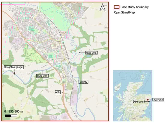
Figure 1.
Case study area of Inverurie, Scotland (Source: Open Street Map).
Inverurie has a long history of fluvial flooding dating back to 1768, with the most notable flood events occurring in November 2002 and January 2016 [26]. The 2002 floods resulted in the highest water level ever recorded, resulting in significant flooding to multiple properties. Across two significant events in January 2016, following Storm Frank, over 80 properties were reported damaged in Inverurie, necessitating evacuation efforts and closure of a number of key transport routes [27]. Given its distinct vulnerability to flooding and long history of severe flood events, Inverurie provides a useful case study for this research.
2.2. Methodology
Figure 2 illustrates the overall research methodology. Observed river flows were extracted from the National River Flow Archive (NRFA) database [25] for the baseline period (1990–2020), and projected flows were extracted from the Earth System Grid Federation (ESGF) across the baseline, near future and far future time horizons (1990–2100). Extreme value (EV) analysis was undertaken on the observed flows, while flow projections were transformed onto the relevant river catchment and bias-corrected to the observed flows across the baseline period (1990–2020), producing the projected flow distributions.

Figure 2.
Research method.
Latin Hypercube Sampling (LHS) was used to quantify climate model uncertainty within the projected flow distributions and transformed into inflow hydrographs, producing upper boundary conditions for the hydraulic model. For the probabilistic approach, each of the inflow hydrographs (n = 100) across the time horizons were used within the LISFLOOD-FP hydraulic model. For the deterministic approach, a single upper boundary condition was used, i.e., the inflow hydrograph for the January 2016 flood event. The hydraulic model’s Manning “n” parameter was calibrated using Particle Swarm Optimization (PSO) techniques, the details of which are reported in [4]. This was done using historical flood data recorded from the November 2002 event, where the Manning “n” friction coefficients were fine-tuned across three parameters. PSO allows for iterative improvements in the fit between the observed and modelled results, until the fitting error is minimised. The fitting statistic (FSTAT), the critical success index determined for each grid cell, was calculated for flood extents, and stage errors (SE) were calculated from the SEPA gauged levels recorded at the Haughton gauge. These were calculated to be 0.77 (FSTAT) and 0.11 (SE) [4].
Flooded extents and maximum water depths were extracted from the model outputs across each of the model runs and were converted into damage estimates based on the maximum water depths recorded for each of the affected properties within Inverurie. The total estimated damage for the deterministic (January 2016) event was calculated. The probabilistic damage estimates and associated probabilities were integrated across all model runs to output a single damage estimate. If the integrated probabilistic damage estimate was found to be greater than the deterministic damage estimate, the adaptation tipping point (ATP) was said to have been reached. However, the probabilistic approach recognises the role that uncertainty plays within adaptation decision making and thus refers rather to the probability at which the ATP is exceeded.
Adaptation scenarios were defined on the basis of plausible local and regional actions [27]. The scenarios were represented in the hydraulic model through variations in the input parameters, for example, changes to the Digital Elevation Model (DEM), river bathymetry, friction coefficients or inflow hydrographs. This was done across the relevant time horizon within which these actions could realistically be implemented, and uncertainty was quantified using the approach described above. The adaptation scenarios were also appraised on the basis of reaching or not reaching the defined ATP, making direct reference to their exceedance probabilities. Each exceedance probability was mapped on the adaptation pathways to facilitate comparison between plausible future scenarios under uncertainty.
NRFA: National River Flow Archive; ESGF: Earth System Grid Federation; EV: extreme value; LHS: Latin Hypercube Sampling; PSO: Particle Swarm Optimization; DEM: Digital Elevation Model.
2.2.1. Hydrology: Boundary Conditions
Daily observed flows for the River Don were extracted from the National River Flow Archive (NRFA) [25], and extreme value (EV) analysis was undertaken to identify annual maximum (AMAX) river flows across the baseline period (1990–2020). Maximum Likelihood Estimation (MLE) was used to fit a generalized extreme value (GEV) statistical distribution to produce a flood frequency curve (Appendix A.1), from which the 95% confidence intervals (CIs) were calculated using parametric bootstrapping, ensuring reproducibility. The range of peak flows for the 1:100-year return period was then determined from the flood frequency curve.
The GEV distribution, G(F), is a three-parameter distribution [28] typically used in the UK to estimate extreme river flows at high return periods [29,30] in accordance with the Flood Estimation Handbook (FEH) [31]:
where ξ is the location parameter, μ is the scale parameter, k is the shape parameter and F is the probability of non-exceedance for a defined return period (T) where F = 1–(1/T).
Daily surface runoff (“mrro”) projections for the RCP8.5 scenario were extracted from the ESGF database for the time periods: 1990–2020 (baseline), 2030–2060 (near future) and 2070–2100 (far future) [32]. EURO-CORDEX is a multi-model ensemble (MME) covering the European (EUR-11) domain [33]. Incomplete datasets were screened out to ensure consistency, resulting in a total of 28 regional climate model (RCM)-global climate model (GCM) combinations [Appendix A.2]. The resolution of the EURO-CORDEX MME was 0.11° (≈12.5 km), and daily surface runoff projections were mapped onto polar rotated co-ordinates in EURO-CORDEX, assuming even distribution across cells. Therefore, the models were transformed onto the Don River catchment and projected onto the British National Grid Coordinates Reference System (CRS) as shown in Figure 3 and described by Equation (2):
where Qcat is the flow rate at the catchment scale, Ng is the total number of grid cells the cover the catchment area (14), lg is the grid cell length (≈12.5 km), ρis water density (≈1000 kg/m3), Ai is the fraction of the i-th grid cell and mrroi is the surface runoff of the i-th grid cell. This follows the methodology detailed within [33].
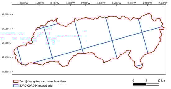
Figure 3.
Transformation of projected flows on the catchment boundary.
Bias correction was performed on each of the 28 RCM-GCM combinations through aggregation and percentile mapping of the projected flows (1990–2100) onto the observed baseline (1990–2020) data extracted for the Haughton gauge from the NRFA. This process applies Percentile Delta Mapping (PDM) to both the observed and projected baseline data by adjusting the projected cumulative density function (CDF) using percentile delta changes between observed and projected flow rates across the baseline period (1990–2020) for each of the 28 ensemble members. This method was chosen over the mean difference or quantile methods as it best captures distributional distances across the range of flows [34]. This process is computationally efficient as it negates the need for catchment-scale modelling [33].
The maximum upper limit and minimum lower limit projected flow rates (m3/s) across the 28 model ensembles for each of the time horizons are summarised in Table A3, Appendix A.3. The range (minimum and maximum values across all 28 ensembles) for each time horizon were extracted, ensuring that all unscreened projections are reflected in the uncertainty quantification process.
2.2.2. Uncertainty Quantification
Latin Hypercube Sampling (LHS), a stratified sampling technique, was used to sample flows across the ensemble ranges. Fewer samples are needed with LHS to obtain convergence whilst maintaining uniformity within the parameter space, when compared with Full Monte Carlo (FMC) methods [4]. In order to construct a normalised hydrograph shape for the upper boundary conditions in the hydraulic model, the January 2016 hydrograph was extracted from the SEPA Online API [35]. The sampled maximum flows were then scaled to produce (n = 100) inflow hydrographs across each of the time horizons.
2.2.3. Hydraulic Model
LISFLOOD-FP, a reduced physics, two-dimensional (2D) model developed to efficiently simulate floodplain inundation, was used for hydraulic (floodplain) modelling [36,37,38,39]. Its reduced physics formulation assists with handling complex topographies over large scales and dynamically simulates the propagation of flood waves across a fluvial floodplain to determine water depths in each grid cell [40].
The 2D model simulates propagation of flood waves along channels and across floodplains by assuming the advection component of the momentum equation is negligible and applying improvements to account for instabilities at large surface friction values [40]:
where q is the flow per unit width (m2/s), h is the flow depth (m), z is the bed elevation (m), g is the acceleration due to gravity (m/s2), n is Manning’s friction coefficient (s/m1/3), t is the time at the current timestep and t + Δt is time at the next timestep (seconds). This flux equation is predicated on the selection of a suitable timestep to ensure that the model stability is maintained for most floodplain flow situations:
where α is a dimensionless coefficient [0.2–0.7] necessary to produce a stable simulation for floodplain flows and Δx horizontal is the cell dimension in the x-direction.
The LISFLOOD-FP base model was created using the acceleration solver for floodplain flow, a computationally efficient finite difference solver represented at a sub-grid resolution [36,37,38,39]. The basic component of the model is the Digital Elevation Model (DEM) created using light detection and ranging (LiDAR) data made available by SEPA [4]. The Manning “n” input raster was created using land cover maps [24] and calibrated through Particle Swarm Optimization (PSO) [4].
To define the boundary conditions, the sampled upstream inflow hydrographs, produced through LHS, were divided by the model resolution (10 m) to generate point-source mass fluxes per unit width (q (m2/s)). The upstream inflows were defined as time-varying, while the downstream boundary condition was modelled as a normal-depth, free boundary to reduce backwater effects, typically experienced when using observed downstream water levels [13]. The boundary condition for the River Urie inflows were modelled as a fixed boundary assuming a constant flow of 10 m3/s, reduced to a point-source fixed mass flux per unit width, q = 1 m2/s. The constant flow assumption of the River Urie was used to isolate the uncertainty related to the River Don and negates the need to undertake joint probability analysis prior to uncertainty quantification. N = 100 models were run for each of the defined time horizons, the outputs from which were converted into probabilistic flooded extents and flood depth hazard maps.
2.2.4. Damage Estimation
Damage curves are a common method to estimate economic loss to properties as a direct function of water depth [41,42,43]. Uncaptured uncertainty in flood hazard analyses, and consequently damage estimates, can lead to poor investment decisions and result in over and under preparedness to respond to future flood hazards. Therefore, uncertainty within the flood hazard analyses was captured in the damage estimations by accounting for the range of water depths and therefore the range of estimated damages experienced by the 1:100-year event.
Property data was extracted from the Scottish Property Database (SPD) within Scotland’s Land Information Service (ScotLIS) [44] and overlayed onto OS Map data in QGIS. The property thresholds were calculated by overlaying the DEM onto the property database, and the properties were classified as per the definitions within the Multi-Coloured Manual (MCM) [45] as presented in Figure 4. Damage curves (as a function of water depth) were derived from the MCM following the UK industry standard approach to economic damage estimation.
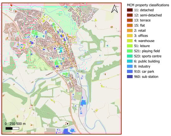
Figure 4.
Property classification according to the MCM [45].
The empirical probability distribution of damages across each time horizon and adaptation scenario were produced, and the probabilities of exceeding the defined adaptation tipping point (ATP) were determined, thereby providing the probabilistic solution across time horizons and scenarios. The objective of flood risk management is explicitly defined by the Local North East Flood Risk Management Plan [27] as “reducing flood risk” or “avoiding an overall increase in risk” relative to the baseline year (2016), where risk is defined as economic losses quantified in terms of total estimated damages (£) incurred in any given year. In contrast, the deterministic solution under risk-based decision making, in any given year, is defined by:
where D(xt) is the polynomial damage curves (from the MCM based on the property classification) as a function of temporally variable water depths (xt) for the affected properties and f(xt) is the fitted continuous probability distribution [6].
The deterministic solutions was computed across all time horizons and scenarios to enable direct comparison with the probabilistic solutions. The application of Equation (5) is predicated on the ability to (i) estimate the time-dependent probability distribution functions f(x) of flooded water depths, (ii) relate water depths to probabilities of flooding where damage may occur and (iii) calculate the damage that is caused by floods of a given magnitude. It also assumes that the flooded system is not significantly sensitive to sub-annual temporal dimensions (such as seasonal variations), and this method ultimately collapses the climate model uncertainty captured through LHS, resulting in a deterministic solution.
The probability functions f(xt) of the water depth distributions were defined, and several goodness-of-fit statistics and criteria were calculated for each scenario across a range of affected grid cells. It was found that 2-parameter Weibull distributions, using the MLE method, fit the water depth distributions most accurately. A 2-parameter Weibull distribution is a continuous probability distribution defined by its shape (k) and scale (λ) as defined by [46]:
The damage within each cell was then summed across the study area to calculate total estimated damages (£) across time horizons and scenarios.
2.2.5. Adaptation Scenarios
A summary of all adaptation scenarios is presented in Table 1, within which the relevant time horizons and adaptation actions are identified. A table of all input parameter modifications and descriptions is enclosed within Appendix B.

Table 1.
Summary of adaptation scenarios, time horizons and actions.
The “No adaptation” scenario represents the future scenario whereby no adaptation actions are implemented. The “Do minimum” scenario represents actions such as the implementation of property-level protection and raised thresholds. This also includes direct flood defences such as 1.5 m flood walls around affected properties. In addition, restoration of the old canal, to provide an additional channel for the flow of water during high-flow conditions, was identified as a relatively cost-effective action and would involve removal of two weirs.
The “storage” scenario represents actions that increase the river and floodplain storage through modifications to the bathymetry of the river channel, setting back of embankments and changes to the floodplain topography. The “woodlands” scenario represents riparian woodland planting. In the near future, it was assumed that the trees will not be fully grown, and therefore a reduced surface friction was used.
A whole-catchment approach, the “land-use management” scenario, represents the implementation of long-term upper catchment land-use management practices to capture surface runoff and increase upstream infiltration, thereby decreasing downstream flows and increasing the time to peak discharge in the far future. A study undertaking catchment-scale modelling of the Tarland catchment found that for a winter 1:100-year event and 15 h storm duration, 100% coniferous afforestation would reduce peak flows by 18% and delay the time to peak by 1 hour [47]. The Tarland catchment is comparable to the Don in terms of location, area, Standard Average Annual Rainfall (SAAR), Base Flow Index (BFI) and standard percentage runoff (SPR). Whole catchment land use change is highly unlikely and the Land Capability for Forestry map [48] indicates that only 19.5% of the Don catchment is classified as having “good” or “moderate” suitability for riparian forestry. This scenario was represented in the hydraulic models as modified inflow hydrographs following resampling using LHS.
These adaptation scenarios were represented within the hydraulic model by modifying the appropriate input parameters, as described in Table A3, Appendix B. The “Do minimum” model included increased Manning coefficients at affected property locations and thresholds across the raster grid cells within to represent property level protection. Grid cell elevations within the DEM were increased by 0.3–1.5 m to account for raised thresholds and impermeable barriers. Canal restoration included incorporating the 1D channel in the flood model and modifications to the DEM and bathymetry (bank, width and bed) input parameters.
The “Storage” model included modifications to the river channel elevations within the DEM and bathymetry parameters by widening the river channel, setting-back the riverbanks and deepening the riverbed depths in locations where increased floodplain storage was viable. These modifications were also undertaken for the “Woodlands” scenario, where riparian woodland planting is represented in the hydraulic model, but included modifications to the Manning coefficients, which represent changes in the surface friction as a result of the increased vegetation.
The “Land-use management” scenario was represented by modifications to the inflow hydrographs through including a decrease in peak flows and a 1-hour delay to peaks across all sampled hydrographs.
3. Results
3.1. Hydrology
Annual maximum (AMAX) discharges (Q) (m3/s) for the baseline period (1991–2020) were extracted for the Don at the Haughton gauge, revealing a maximum peak discharge, Qpeak, of 396.3 m3/s that occurred in January 2016, and the upper and lower limits for the 1:100-year return period were found to be 184.4 m3/s and 733.6 m3/s, respectively.
Figure 5 presents the violin plots for the downscaled and bias-corrected EURO-CORDEX projections, revealing how the distributions of flow rates (m3/s) and associated uncertainties are projected to change over time. Table 2 summarises the transformed and bias-corrected ranges of flow rates used, i.e., the maximum upper limit and minimum lower limit flow rates across the 28 unscreened ensembles, enclosed within Appendix A.3.
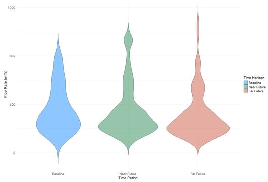
Figure 5.
Violin plot showing the projected flow distributions across time horizons for the 1:100-year return period.
Table 2.
Minimum lower limit and maximum upper limit flow rates (m3/s) across time horizons.
3.2. Probabilistic Hazard Maps
Figure 6 presents the deterministic and probabilistic flood hazard maps (flood extents and maximum water depths) for the 1:100-year return period, revealing the spatial and temporal distributions of flood risk across the case study region and across time horizons. While mapping probabilistic flood extents has been demonstrated by several authors, probabilistic representation of flood depths is less common, and Figure 6 presents the range of flood depths in the deterministic solution as well as the probability of maximum flood depths categorised within four continuous ranges, i.e., <0.3 m, 0.3–1 m, 1–2 m and >2 m, computed across each of the time horizons.
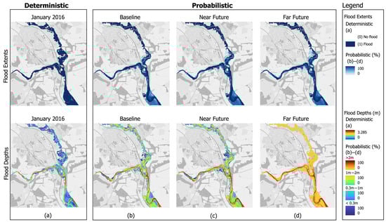
Figure 6.
Deterministic flood extents and depths (a) and probabilistic flood extents and depths across the baseline (b), near future (c) and far future (d).
The deterministic maps (Figure 6a) show a single flood extent and maximum water depth output for the January 2016 event. In contrast, the probabilistic maps (baseline (Figure 6b), near future (Figure 6c) and far future (Figure 6d)) capture uncertainty within the flood extents and depths. Probabilistic flood extents (top row) demonstrate increasing spatial coverage of inundation over time, with the far future scenario showing the greatest extent and highest likelihood of flooding across the floodplain. Probabilistic flood depths (bottom row) also reveal a clear intensification of flood hazard over time, with deeper floodwaters (>2 m) becoming increasingly probable, especially along river-adjacent and low-lying areas.
These results highlight the growing exposure of Inverurie to more severe and widespread fluvial flooding under future climate scenarios. Moreover, they illustrate the additional insight gained through probabilistic modelling, particularly in capturing spatial distributions of flood risk and identifying areas where the likelihood of extreme flood depths significantly increases across time horizons.
3.3. Damage Estimation
Using the property classification method prescribed by the MCM and applying the polynomial expressions for a long duration storm event assuming no early warning, flood damages (£) as a function of maximum flood depths (m) were calculated for the January 2016 event and across time horizons and adaptation scenarios. The January 2016 event is defined explicitly as the adaptation tipping point (ATP) against which future risks (damages) are compared. The total estimated damage of the January 2016 event was calculated to be £147,933.66. The performance of the base (January 2016) hydraulic model was evaluated by comparing simulated flood extents and depths with observed data from the January 2016 event. In terms of damages, the model demonstrated a strong performance, achieving an agreement of 0.88 between observed flood damages attributed to fluvial flooding and the modelled base-year results [27]. To compute the deterministic solutions across time horizons and scenarios, the product of damages within each grid cell were fitted to suitable probability distributions (Equation (6)) integrated across distributions (Equation (5)) and summed across all affected grid cells within the case study area.
Figure 7 presents the spatial distribution of theoretical flood damages (£) across various adaptation scenarios and future time horizons. Theoretical damages were computed by integrating depth–damage curves, derived from the MCM property classification, with appropriately fitted probability distributions (Equation (5)), resulting in deterministic estimates of total damages. Figure 7 presents the spatial distribution of damages across the case study area using a graduated red scale, where higher intensities represent greater estimated damages.
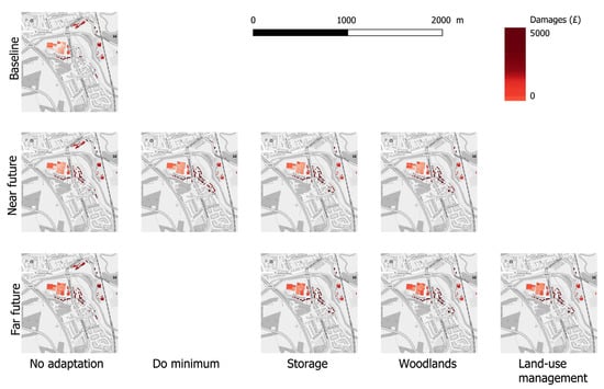
Figure 7.
Spatial distribution of theoretical total estimated damage (£) across scenarios and time horizons.
While spatial patterns of damage remain broadly consistent across all scenarios, with the most affected areas appearing repeatedly, there are subtle yet important differences in both the extent and intensity of fluvial flooding. These variations, although not visually discernible at the 10 m resolution, are reflected in the total damage estimates provided in Table 3.
Table 3.
Total damages (£) across the case study area for each scenario and time horizon.
Table 3 summarises total theoretical damages for each scenario and time horizon. The results indicate that, under the deterministic solution, none of the adaptation strategies achieve a reduction in total damages relative to the ATP, i.e., the January 2016 event. This is reflected in adaptation pathways as binary termination points (see Section 3.4 and Figure 8); however, the “no adaptation” scenario yields the highest total damages in both the near and far future, revealing the potential benefit of adaptive interventions.
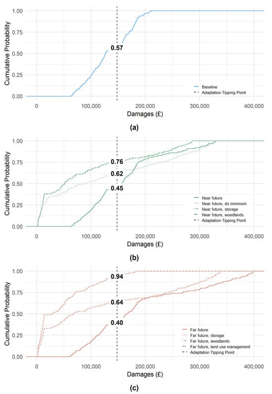
Figure 8.
Empirical cumulative probability distribution of damages (£) for the baseline (a), near future (b) and far future (c).
Although the adaptation scenarios offer some mitigation of future flood damages, particularly in the near future, the deterministic solutions do not capture the relative probabilities of exceeding the ATP. Therefore, while useful for understanding cumulative potential damages of fluvial flooding, the results ought to be presented within a probabilistic framework to fully evaluate adaptation performance.
3.4. Adaptation Pathways
The probabilistic solutions were plotted as empirical cumulative density functions (CDFs), highlighting the probability of each adaptation scenario reaching the defined ATP, as shown in Figure 8. The explicit definition of the ATP is the January 2016 total flood damages (£), calculated at £147,933.66. Figure 8 also presents numerical values on the CDF curves at the ATP thresholds, which represent the non-exceedance probabilities for each scenario, i.e., the probabilities that damages will remain below the ATP.
This facilitates the development of adaptation pathways across time horizons and allows for a direct comparison of exceedance probabilities within the probabilistic solution, as presented in Figure 9, and identification of binary termination points within the deterministic solution. The probabilistic solution prescribes a probability of exceedance on the basis of:
where F(x) = P(X ≤ x) is the CDF (or non-exceedance probability), x = ATP (£) and () is the exceedance probability. Ultimately, this demonstrates the method through which climate model uncertainty can be quantified within the development of adaptation pathways, i.e., through calculation of the ATP exceedance probabilities (EP(x)). The tipping points are defined as the points where flood damages exceed the ATP, and the numbers indicated on the curves reflect the likelihood of remaining below this critical threshold. This enables direct comparison of probabilistic performance between scenarios across time horizons.
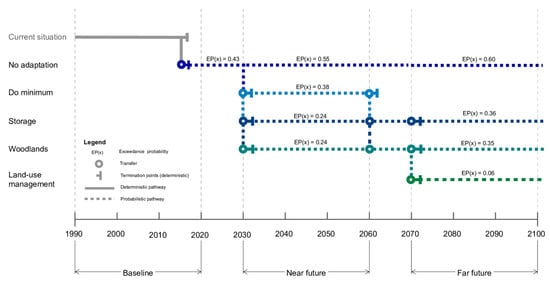
Figure 9.
Adaption pathways identifying deterministic termination points (deterministic), adaptation tipping point exceedance probabilities (probabilistic).
Figure 9 presents the adaptation pathways, identifying multiple combinations of sequences of actions that can be taken across the baseline, near future and far future. The EP(x) values represent a probabilistic performance threshold, i.e., how well each strategy performs in reducing flood risk (in terms of exceedance probabilities). The termination points represent points in time where the deterministic solution, i.e., the integral of the product of damages and probabilities across time horizons, exceeds the base year level of risk (in damages (£)). The pathways depict how adaptation actions can be implemented in sequence, with transfer points indicating when a switch to another action is, or may be, needed. In this way, the pathways allow for flexibility and transitions between actions, removing inherent path dependency and identifying pathways that maintain an acceptable level of risk.
4. Discussion
4.1. Hydrology
An assessment of the future climate hydrology for the River Don reveals a distribution of flow rates for the 1:100-year return period event across time horizons. The violin plots reveal a baseline distribution across RCMs concentrated around lower values (200–400 m3/s), with larger spread in the lower range, tapering towards higher flow rates. The near future distribution has a slightly broader spread with a secondary peak identified (800–900 m3/s), suggesting an increase in extreme flows and indicating larger uncertainty compared to the baseline. The far future projections have the widest distribution, with an extended tail reaching higher extreme flow rates, thereby shifting the central tendency upwards. This reveals that climate model uncertainty and extreme maximum flows increase as the time horizon increases. RCP8.5 has the largest model distribution and therefore captures the largest uncertainty, generally increasing across time horizons, suggesting that flood risk becomes increasingly more uncertain in the future under an RCP8.5 scenario.
4.2. Probabilistic Hazard Maps
The projected flow distributions are reflected in the probabilistic hazard maps, whereby flood extents and depths increase as time horizons increase for the 1:100-year event. The far future scenario has the largest flood extents, indicating that climate-induced increases in fluvial flows contribute to a greater flood-prone area. In addition, uncertainty, captured through the probability of flooding to each affected grid cell, is greater for all scenarios when compared to the deterministic solution and also depicts an increasing trend across time horizons. The far future scenario shows the highest climate model uncertainty, concurring with the results of the hydrological analysis.
The deterministic flood depths show significant flooding along the river channel and adjacent floodplains, generally in agreement with observations recorded following the January 2016 storm event. The probabilistic flood depths show an increase in magnitude and extent over time, with the baseline depicting lower flood depths concentrated near the river channel, while the near future reveals an increase in flood depths and higher water depths (>2 m) within low-lying areas, and the far future reveals more widespread and deeper flooding across large areas, with water depths exceeding 2 m.
The probabilistic hazard maps suggest that flood risk is projected to increase over time, both in extent and depth, with increasing climate model uncertainty and therefore increased risk as time horizons increase. The probabilistic projections provide a more robust assessment of flood risk across time horizons, indicating a range of possible flood outcomes through the capturing of uncertainty, thereby assisting decision making through identification of the likelihood of flooding in conjunction with magnitude. This could improve prioritisation of adaptation actions and supports a more flexible and adaptive approach to flood risk management, accounting for a range of future conditions.
4.3. Damage Estimation
An evaluation of the spatial distribution of flood damages, presented in Figure 7, indicates that the majority of damage is concentrated between the A96 and the railway line, primarily upstream of the confluence of the Rivers Don and Urie. This area includes a mix of land uses: open fields, a sports club, a wastewater treatment facility, and a number of residential and commercial properties.
Across all time horizons, total estimated damages increase significantly, particularly under the “no adaptation” scenario. Table 3 quantifies total damages, demonstrating that while none of the tested adaptation strategies fully mitigate damages to levels observed during the January 2016 event (ATP), all scenarios offer some degree of reduction compared to the “no adaptation” pathway. This trend is particularly evident in the near future, where strategies such as implementing riparian floodplain storage and woodland planting yield notable reductions in expected damages.
The damage estimation process involved the integration of depth–damage curves, derived from the Multi-Coloured Manual (MCM) property classifications, and the relevant fitted probability distributions for each scenario. While this deterministic approach provides valuable insights into potential spatial and temporal flood damage patterns, it has notable limitations. The fitted probability distributions do not account for the full range of variability and uncertainty across time horizons and scenarios. This restricts the ability of the analysis to evaluate the likelihood of exceeding the ATP and underrepresents the probabilistic nature of future flood risks.
Furthermore, the use of MCM depth–damage curves introduce variability in estimated damages based on property type and classification. This means that even when properties experience similar water depths, the resulting damages can differ substantially due to differences in structural vulnerability, use and asset value, introducing an additional layer of complexity, especially when interpreting spatial distribution of flooding across a heterogeneous area.
While the deterministic framework enables a comparative evaluation of adaptation performance and highlights key at-risk areas, the probabilistic approach, whereby uncertainty is captured in the solution, allows for a more robust comparison of adaptation scenario performances based on event likelihood and probabilities of exceeding the defined ATP.
4.4. Adaptation Pathways
Figure 8 and Figure 9 illustrate how combining adaptation pathway mapping with empirical cumulative distribution functions (CDFs) and identification of exceedance probabilities (EP(x)) enables a more dynamic and risk-informed decision-making framework.
Figure 8 presents empirical cumulative distribution functions (CDFs) for the baseline, near future and far future time horizons, showing the probability distributions of flood damages under various adaptation scenarios. The use of a defined adaptation tipping points (ATP) enables direct comparison between scenarios. The exceedance probability at the ATP reflects the likelihood that damages will exceed the defined threshold. The ATP was determined based on total damages during the January 2016 flood event, providing a context-specific threshold for unacceptable risk. The numbers indicated on the CDF curves represent the cumulative probabilities of non-exceedance at the ATP, allowing for a clear interpretation of how likely each scenario is to stay below this risk threshold. For instance, in the far future, a “no adaptation” approach leads to a 60% probability of exceeding the ATP (40% cumulative probability of non-exceedance), while the introduction of “land-use management” reduces this risk to just 6% (94% cumulative probability of non-exceedance). This quantification of exceedance probabilities (EP(x)) under each scenario enables decision makers to assess the relative effectiveness of interventions, not just in deterministic terms but across a full range of possible outcomes.
Figure 9 presents a suite of probabilistic adaptation pathways, each quantified using exceedance probabilities (EP(x)) of reaching the defined adaptation tipping point (ATP). Unlike deterministic models that simply identify binary thresholds, this approach assigns a probability of exceedance to each strategy at different points in time. For instance, the “no adaptation” pathway depicting increasing EP(x) values over time highlights growing exposure to flood risk. In contrast, strategies such as “storage” and “woodlands” reduce EP(x) significantly in the near future (24%), while “land-use management” emerges as the most robust long-term solution, achieving an EP(x) of just 6% by 2070. This quantification enables a meaningful comparison between adaptation scenarios across time horizons.
In contrast, the deterministic solution, which integrates all potential damages and their associated probabilities over time, results in fixed termination points that indicate no single adaptation action, nor sequence of actions, in the near or far future can permanently prevent exceedance of the ATP, thereby falling short of fully mitigating long-term flood risk. This illustrates the difference between probabilistic and deterministic approaches: while deterministic results indicate when risk thresholds are crossed, probabilistic methods provide insight into how probable this is to occur across different scenarios and periods, underscoring the importance of probabilistic approaches to flood risk management.
Together, Figure 8 and Figure 9 demonstrate that embedding climate model uncertainty into adaptation pathways enables more informed, risk-based decision making. Rather than relying on deterministic decision making, different actions can be assessed based on their probabilistic performance across a range of future conditions while preserving flexibility to adapt over time. The probabilistic solution enables identification of plausible future pathways that maintain an acceptable level of risk while allowing flexibility and robustness in decision making under uncertainty.
Finally, these results indicate that adaptation pathways are influenced by the decision context within which the ATPs are defined. Therefore, careful consideration of the selection of appropriate ATPs is recommended to ensure that decisions are made in an informed and consistent manner so as to ensure that the adaptation objectives can be quantified. Climate change under the RCP8.5 climate scenario demonstrates challenges to achieving an overall avoidance of risk in the future when implementing a deterministic approach to decision making; however, through a probabilistic approach, adaptation actions can be suitably appraised through their ability to reduce the exceedance probabilities.
4.5. Further Work
Given the inherent complexity and uncertainty related to the climate models, modelling using alternative climate projections would further validate this methodology. A range of emission scenarios (including RCP2.6 and 4.5) could be considered [49], the outputs from which could be compared with the RCP8.5 scenario. In addition, checking for overfitting for the bias correction of the projections to the observed data is recommended, the results of which could be compared across several bias correction methods.
This research has only considered a 1:100-year return period; however, a range of return periods could be considered (e.g., 1:10, 1:30, 1:200, 1:1000). This would increase the spread of the distributions and therefore uncertainty of the water depths and damages, and the theoretical risk function could be used to integrate across multiple return periods to give a wider spread of data across various magnitudes. In addition, the damage functions could include damage to agricultural land, woodlands, roads, railways, and other critical infrastructure.
The number of samples taken across projected peak flow distributions could be increased from n = 100 to n = 10,000 to ensure a wider and more accurate spread. This would result in a significant increase in model runs and would be computationally more onerous. However, alternative methods of uncertainty quantification, such as Multi-Level Monte Carlo (MLMC) methods [4] or the building of emulators, could be used [30]. In addition, the hydraulic models could be run at a higher resolution (5 m × 5 m) to improve the accuracy of outputs.
Future research could analyse several alternative adaptation actions that integrate engineered solutions and natural flood management (NFM), for which economic appraisals using Cost–Benefit Analysis (CBA) or real options analysis (ROA) could be undertaken. Since the climate projections indicate potential low-flow conditions in the far future, future work could assess the robustness of adaptation options across both high and low flows.
Finally, the success of adaptation depends largely on the vulnerabilities and capabilities of the local community to respond to flood hazards [50]. Therefore, engaging with and understanding the needs of the local community and involving them in the decision-making process is integral to achieving transformational adaptation. A “bottom-up” approach could be compared with the “top-down” approach presented in this research and should include community and stakeholder engagement and elucidation, quantitative or qualitative assessments of vulnerability and assessment of multi-benefits and unquantifiable (or intangible) benefits of flood risk management, not only from an economic perspective but also from environmental and social anthropogenic perspectives.
4.6. Assumptions and Limitations
To isolate the uncertainty attributed to the climate models, other drivers (e.g., population growth) have not been included in the hydraulic models. In addition, non-fluvial hydrological processes such as evaporation, transpiration and groundwater flows have not been hydraulically modelled; however, these are not routinely included in hydraulic simulations of floodplain inundation. Isolation of climate model uncertainty in the hydraulic models allowed for consideration of a theoretical system whereby other sources of uncertainty are appropriately managed and are assumed to be negligible relative to climate model uncertainty [5].
An identified limitation of uncertainty quantification is the computational burden of running a sufficiently large sample of model realisations [11]. This research has used n = 100 iterations to quantify uncertainty using a stratified approach. Full Monto Carlo simulations are often considered to be the “gold standard” approach; however, this requires a larger sample size (e.g., n = 10,000) to ensure the full input distribution uncertainty is captured.
Damage estimation was undertaken in accordance with the MCM [45], accounting for direct damages, measured in terms of 2019–2020 prices. This makes the relative damages across the scenarios directly comparable. However, damage estimation only considered impacts to residential and non-residential properties and did not account for damage to agricultural land and transportation infrastructure, for which there is limited empirical data to derive damage curves. Similarly, indirect damages or damages to natural assets and the environment were not included. In reality, flood damages depend not only on inundation extent and water depth but also velocity, duration of inundation, sediment concentration as well as the communication of flood warnings. However, this paper excludes such factors as there are limited data available.
Real options theory builds upon financial options theory, whereby investment decisions are appraised in terms of net present costs and benefits by applying an appropriate discount factor. It is an alternative approach to cost–benefit analyses (CBA), explicitly accounting for uncertainty for robust decision making [51]. This calculates the (net present) costs of adaptation actions (including capital, operation, maintenance, replacement and decommissioning costs) [52] and often uses “damages avoided” for the basis of the quantification of benefits [53]. Additionally, the comparison of economic value of risk proposes a simplified approach to informing flood management decisions; however, this fails to consider other more complex decision criteria, such as costs to human life, environmental costs, safety, public health and social impacts of floods, the quantification of which would be subject to unquantifiable uncertainties [6].
5. Conclusions
This research has demonstrated that probabilistic approaches to flood risk management can be used to inform adaptation pathways, and that in doing so, different decisions may be taken. It presents a methodology to quantify and capture climate model uncertainty in adaptation pathways for multiple plausible adaptation scenarios across three 30-year time horizons (baseline, near future and far future). Uncertainty is quantified using Latin Hypercube Sampling and captured across hydraulic models, resulting in the identification of adaptation actions and subsequent pathways within the context of a specified flood risk management objective.
The impact of the quantified climate model uncertainty on adaptation pathways is demonstrated through the quantification of exceedance probabilities relative to defined adaptation tipping points across a range of adaptation scenarios and time horizons. This research has identified how climate model uncertainty can be captured in adaptation pathways and subsequently be used to inform decisions on the selection of an appropriate pathway that minimises the probabilities of exceedance. It discusses potential considerations that influence the chosen adaptation pathway in the context of uncertainty.
The results indicate that adaptation pathways are influenced by the type of function fitted to the maximum flood water depth distributions in the deterministic solution and discusses how the decision context may influence the identification of adaptation tipping points. Ultimately, by quantifying climate model uncertainty in adaptation pathways, this study enables more robust, adaptive decision making over multiple time horizons. This research concludes that uncertainty could be embraced in flood risk decision making, particularly to inform adaptation pathways. By quantifying climate model uncertainty in adaptation pathways, decisions can be made about adaptation actions across a range of time horizons, which are different to those made under deterministic modelling. These decisions could support inclusive, “bottom-up” planning decisions in a risk-informed manner.
Author Contributions
Conceptualisation, J.D., W.R. and L.B.; methodology, J.D. and L.B.; software, J.D. and W.R.; validation, J.D. and W.R.; formal analysis, J.D. and W.R.; investigation, J.D. and W.R.; resources, J.D., W.R. and L.B.; data curation, J.D. and W.R.; writing—original draft preparation, J.D.; writing—review and editing, L.B.; visualisation, J.D.; supervision, L.B.; project administration, L.B. All authors have read and agreed to the published version of the manuscript.
Funding
This work was supported by EPSRC EP/X041093/1.
Data Availability Statement
The original data presented in the study are openly available in Zenodo at https://doi.org/10.5281/zenodo.15195618.
Acknowledgments
River flow data and the catchment shapefiles were extracted from the UK National River Flow Archive (NRFA) (National River Flow Archive), flow projections were extracted from the Earth System Grid Federation (ESGF) search portal (CEDA ESGF Search Portal|ESGF-CEDA|ESGF-CoG), the 15-min time series data were extracted from Scottish Environment Protection Agency’s (SEPA) online API (SEPA Time series data service (API)|Scottish Environment Protection Agency|SEPA), property data were extracted from Scotland’s Land Information Service (ScotLIS) (ScotLIS—Registers of Scotland) and LISFLOOD-FP were downloaded from SEAMLESS-WAVE (LISFLOOD-FP8.0|SEAMLESS-WAVE).
Conflicts of Interest
The authors declare no conflicts of interest.
Abbreviations
The following abbreviations are used in this manuscript:
| AMAX | Annual maximum |
| ATP | Adaptation tipping point |
| BFI | Base Flow Index |
| CBA | Cost–benefit analyses |
| CDF | Cumulative density function |
| CI | Confidence interval |
| CMIP | Coupled Model Intercomparison Project |
| CORDEX | Coordinated Regional Climate Downscaling EXperiment |
| CRS | Coordinates Reference System |
| DEM | Digital Elevation Model |
| EV | Extreme value |
| ESGF | Earth System Grid Federation |
| FEH | Flood Estimation Handbook |
| FMC | Full Monte Carlo |
| GCM | General Circulation Model |
| GEV | Generalised extreme value |
| GHG | Greenhouse gas |
| HOST | Hydrology of Soil Types |
| LHS | Latin Hypercube Sampling |
| MC | Monte Carlo |
| MCM | Multi-Coloured Manual |
| MLE | Maximum Likelihood Estimation |
| NRFA | National River Flow Archive |
| NFM | Natural flood management |
| Probability density function | |
| PFM | Probabilistic flood map |
| RCM | Regional climate model |
| RCP | Representative Concentration Pathway |
| ROA | Real options analysis |
| SAAR | Average annual rainfall in the standard period (1961–1990) |
| ScotLIS | Scotland Land Information Service |
| SPD | Scottish Property Database |
| SPR | Standard percentage runoff |
| SEPA | Scottish Environmental Protection Agency |
| TFRCD | Task Force for Regional Climate Downscaling |
| UKCEH | UK Centre for Ecology & Hydrology |
| WCRP | World Climate Research Programme |
Appendix A
Appendix A.1
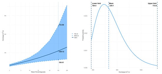
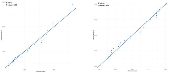
Figure A1.
Extreme value analysis.
Appendix A.2
Table A1.
EURO-CORDEX GCM-RCM combinations.
Table A1.
EURO-CORDEX GCM-RCM combinations.
| Driving Model (GCM) | Institution | RCM |
|---|---|---|
| ICHEC-EC-EARTH | CLM (Climate-Limited Area Modelling) | CCLM4-8-17_1 |
| data | CCLM4-8-17_3 | |
| CCLM4-8-17_4 | ||
| CCLM4-8-17_5 | ||
| KNMI (Koninklijk Nederlands Metrologisch Institute) | RACMO22E_2 | |
| RACMO22E_3 | ||
| RACMO22E_4 | ||
| RACMO22E_5 RACMO22E_6 | ||
| CLM (Climate-Limited Area Modelling) | COSMO-crCLIM-v1-1_1 | |
| COSMO-crCLIM-v1-1_2 | ||
| COSMO-crCLIM-v1-1_3 | ||
| COSMO-crCLIM-v1-1_4 | ||
| MOHC (Met Office Hadley Centre) | HadREM3-GA7-05_1 | |
| HadREM3-GA7-05_3 | ||
| HadREM3-GA7-05_4 | ||
| DMI (Danmarks Meterologiske Institut) | HIRHAM5_1 | |
| HIRHAM5_2 | ||
| HIRHAM5_3 | ||
| HIRHAM5_5 | ||
| HIRHAM5_6 | ||
| MPI-ESM1-M | MPI-M (Max Planck Institute for Meteorology) | REMO2009 |
| NCC-NorESM1-M | GERICS (Climate Service Center Germany) | REMO2015_2 |
| REMO2015_3 | ||
| REMO2015_4 | ||
| REMO2015_5 | ||
| REMO2015_6 | ||
| REMO2015_7 |
Appendix A.3
Table A2.
Minimum lower limit and maximum upper limit flow rates (m3/s) across each climate model for each time horizon.
Table A2.
Minimum lower limit and maximum upper limit flow rates (m3/s) across each climate model for each time horizon.
| Climate Model | Baseline | Near Future | Far Future | |||
|---|---|---|---|---|---|---|
| Min. Lower (m3/s) | Max. Upper (m3/s) | Min. Lower (m3/s) | Max. Upper (m3/s) | Min. Lower (m3/s) | Max. Upper (m3/s) | |
| CCLM4-8-17_1 | 192.9 | 378.2 | 172.9 | 397.8 | 121.0 | 209.9 |
| CCLM4-8-17_3 | 175.1 | 407.9 | 149.1 | 502.9 | 131.4 | 574.4 |
| CCLM4-8-17_4 | 186.5 | 471.7 | 158.1 | 366.0 | 139.4 | 290.3 |
| CCLM4-8-17_5 | 173.6 | 582.9 | 160.8 | 233.8 | 109.8 | 170.2 |
| RACMO22E_2 | 212.9 | 563.7 | 219.6 | 928.9 | 137.6 | 652.0 |
| RACMO22E_3 | 225.2 | 601.6 | 211.2 | 317.2 | 167.5 | 718.0 |
| RACMO22E_4 | 170.3 | 621.1 | 135.4 | 228.6 | 119.9 | 355.7 |
| RACMO22E_5 | 222.8 | 754.3 | 190.9 | 617.3 | 123.0 | 455.9 |
| RACMO22E_6 | ||||||
| COSMO-crCLIM-v1-1_1 | 184.1 | 490.2 | 172.0 | 263.2 | 181.7 | 368.5 |
| COSMO-crCLIM-v1-1_2 | 161.5 | 526.8 | 185.4 | 554.9 | 216.9 | 754.8 |
| COSMO-crCLIM-v1-1_3 | 193.6 | 688.9 | 192.2 | 614.8 | 194.1 | 365.2 |
| COSMO-crCLIM-v1-1_4 | 200.1 | 474.1 | 216.7 | 733.4 | 198.8 | 491.9 |
| HadREM3-GA7-05_1 | 213.4 | 444.4 | 218.7 | 380.5 | 229.5 | 338.5 |
| HadREM3-GA7-05_3 | 156.2 | 422.6 | 153.1 | 279.1 | 185.9 | 767.2 |
| HadREM3-GA7-05_4 | 187.2 | 665.9 | 211.2 | 544.9 | 187.1 | 243.6 |
| HIRHAM5_1 | 197.4 | 427.3 | 205.7 | 325.5 | 209.9 | 396.5 |
| HIRHAM5_2 | 125.5 | 765.5 | 128.1 | 619.5 | 226.8 | 1075.9 |
| HIRHAM5_3 | 135.6 | 763.2 | 133.7 | 356.1 | 135.9 | 489.8 |
| HIRHAM5_5 | 163.5 | 771.6 | 243.1 | 928.9 | 123.7 | 251.6 |
| HIRHAM5_6 | 134.3 | 762.4 | 129.7 | 928.9 | 135.8 | 556.8 |
| REMO2009 | 124.0 | 647.8 | 169.6 | 795.9 | 172.5 | 595.6 |
| REMO2015_2 | 198.4 | 593.9 | 222.5 | 664.7 | 219.3 | 489.3 |
| REMO2015_3 | 199.9 | 656.9 | 196.7 | 343.6 | 209.4 | 573.8 |
| REMO2015_4 | 183.6 | 575.0 | 210.0 | 928.9 | 167.0 | 198.2 |
| REMO2015_5 | 195.8 | 595.8 | 235.1 | 464.3 | 240.4 | 542.5 |
| REMO2015_6 | 219.0 | 777.8 | 210.5 | 583.9 | 208.4 | 561.7 |
| REMO2015_7 | 197.7 | 550.9 | 245.6 | 928.9 | 207.5 | 501.8 |
| Min lower limit | 124.0 | 128.1 | 109.8 | |||
| Max. upper limit | 777.8 | 928.9 | 1075.9 | |||
Appendix B
Table A3.
Adaptation scenarios, actions, modified parameters and description of modifications.
Table A3.
Adaptation scenarios, actions, modified parameters and description of modifications.
| Scenario | Time Horizon | Adaptation Actions | Modified Parameters | Description |
|---|---|---|---|---|
| No adaptation | Baseline Near future Far future | None | None | None |
| Do minimum | Near future | Direct defences | DEM, Manning “n” | Levels raised by 1.5 m at location of proposed walls to the WWTP and commercial properties Residential property thresholds raised by 0.3 m N = 1 for impermeable barriers |
| Old canal restoration | DEM, bed, width, bank, Manning “n” | Includes the old canal channel N = 0.05 | ||
| Storage | Near future Far future | Increase floodplain storage | DEM, bed, width, bank, Manning “n” | Uniformly reduced elevations relative to the river channel elevations Setting back and reprofiling of embankments N = 0.05 |
| Woodlands | Near future Far future | Riparian woodland creation along the riverbanks | DEM, bed, width, bank, Manning “n” | As above N = 0.06 (near future); n = 0.1 (far future) |
| Land-use management | Far future | Whole-catchment woodland creation | Upstream inflows | Reduced peak flow by 3.5% Delay to peak flow by 1 h |
Table A4.
Theoretical (deterministic) damages (£) across adaptation scenarios.
Table A4.
Theoretical (deterministic) damages (£) across adaptation scenarios.
| Scenario | Time Horizon | Total Estimated Damage (£) | Exceeds ATP? |
|---|---|---|---|
| ATP | January 2016 | 147,933.66 | |
| No adaptation | Baseline | 175,576.20 | Y |
| Near future | 273,502.31 | Y | |
| Far future | 228,929.28 | Y | |
| Do minimum | Near future | 261,469.62 | Y |
| Storage | Near future | 224,552.60 | Y |
| Far future | 153,918.23 | Y | |
| Woodlands | Near future | 224,740.00 | Y |
| Far future | 163,360.93 | Y | |
| Land-use management | Far future | 159,968.55 | Y |
References
- Ritchie, H.; Rosado, P. Global Damage Costs from Natural Disasters. Natural Disasters. Available online: https://ourworldindata.org/grapher/damage-costs-from-natural-disasters (accessed on 2 August 2024).
- Sayers, P.B.; Horritt, M.S.; Penning-Rowsell, E.; Mckenzie, A. Climate Change Risk Assessment 2017: Projections of Future Flood Risk in the UK. 2015. Available online: www.sayersandpartners.co.uk (accessed on 18 January 2025).
- Caretta, M.A.; Mukherji, A.; Arfanuzzaman, M.; Betts, R.A.; Gelfan, A.; Hirabayashi, Y.; Lissner, T.K.; Liu, J.; Gunn, E.L.; Morgan, R.; et al. Water. In Climate Change 2022: Impacts, Adaptation and Vulnerability; Contribution of Working Group II to the Sixth Assessment Report of the Intergovernmental Panel on Climate Change; Cambridge University Press: Cambridge, UK; New York, NY, USA, 2022; pp. 551–712. [Google Scholar] [CrossRef]
- Aitken, G.; Beevers, L.; Christie, M.A. Multi-Level Monte Carlo Models for Flood Inundation Uncertainty Quantification. Water Resour. Res. 2022, 58, e2022WR032599. [Google Scholar] [CrossRef]
- Beevers, L.; Collet, L.; Aitken, G.; Maravat, C.; Visser, A. The influence of climate model uncertainty on fluvial flood hazard estimation. Nat. Hazards 2020, 104, 2489–2510. [Google Scholar] [CrossRef]
- Hall, J.; Solomatine, D. A framework for uncertainty analysis in flood risk management decisions. Int. J. River Basin Manag. 2008, 6, 85–98. [Google Scholar] [CrossRef]
- Di Baldassarre, G.; Montanari, A. Hydrology and Earth System Sciences Uncertainty in River Discharge Observations: A Quantitative Analysis. 2009. Available online: www.hydrol-earth-syst-sci.net/13/913/2009/ (accessed on 15 July 2024).
- Collet, L.; Beevers, L.; Stewart, M.D. Decision-Making and Flood Risk Uncertainty: Statistical Data Set Analysis for Flood Risk Assessment. Water Resour. Res. 2018, 54, 7291–7308. [Google Scholar] [CrossRef]
- Di Baldassarre, G.; Schumann, G.; Bates, P.D.; Freer, J.E.; Beven, K.J. Cartographie de zone inondable: Un examen critique d’approches déterministe et probabiliste. Hydrol. Sci. J. 2010, 55, 364–376. [Google Scholar] [CrossRef]
- Horritt, M.S.; Di Baldassarre, G.; Bates, P.D.; Brath, A. Comparing the performance of a 2-D finite element and a 2-D finite volume model of floodplain inundation using airborne SAR imagery. Hydrol. Process. 2007, 21, 2745–2759. [Google Scholar] [CrossRef]
- Teng, J.; Jakeman, A.J.; Vaze, J.; Croke, B.F.W.; Dutta, D.; Kim, S. Flood Inundation Modelling: A Review of Methods, Recent Advances and Uncertainty Analysis; Elsevier Ltd.: Amsterdam, The Netherlands, 2017. [Google Scholar] [CrossRef]
- Collet, L.; Beevers, L.; Prudhomme, C. Assessing the impact of climate change and extreme value uncertainty to extreme flows across Great Britain. Water 2017, 9, 103. [Google Scholar] [CrossRef]
- Horritt, M.S. A methodology for the validation of uncertain flood inundation models. J. Hydrol. 2006, 326, 153–165. [Google Scholar] [CrossRef]
- European Parliament and Council. Directive 2007/60/EC on the Assessment and Management of Flood Risk. 2007. Available online: https://eur-lex.europa.eu/legal-content/EN/TXT/?uri=CELEX:32007L0060 (accessed on 2 June 2024).
- Clark, M.P.; Wilby, R.L.; Gutmann, E.D.; Vano, J.A.; Gangopadhyay, S.; Wood, A.W.; Fowler, H.J.; Prudhomme, C.; Arnold, J.R.; Brekke, L.D. Characterizing Uncertainty of the Hydrologic Impacts of Climate Change; Springer: Berlin, Germany, 2016. [Google Scholar] [CrossRef]
- Sparkes, E.; Totin, E.; Werners, S.E.; Wise, R.M.; Butler, J.R.A.; Vincent, K. Adaptation pathways to inform policy and practice in the context of development. Env. Sci. Policy 2023, 140, 279–285. [Google Scholar] [CrossRef]
- Werners, S.E.; Wise, R.M.; Butler, J.R.A.; Totin, E.; Vincent, K. Adaptation Pathways: A Review of Approaches and a Learning Framework; Elsevier Ltd.: Amsterdam, The Netherlands, 2021. [Google Scholar] [CrossRef]
- Haasnoot, M.; Middelkoop, H.; Offermans, A.; van Beek, E.; van Deursen, W.P.A. Exploring pathways for sustainable water management in river deltas in a changing environment. Clim. Change 2012, 115, 795–819. [Google Scholar] [CrossRef]
- Haasnoot, M.; Kwakkel, J.H.; Walker, W.E.; Maat, J.T. Dynamic adaptive policy pathways: A method for crafting robust decisions for a deeply uncertain world. Glob. Environ. Change 2013, 23, 485–498. [Google Scholar] [CrossRef]
- Lin, B.B.; Capon, T.; Langston, A.; Taylor, B.; Wise, R.; Williams, R.; Lazarow, N. Adaptation Pathways in Coastal Case Studies: Lessons Learned and Future Directions. Coast. Manag. 2017, 45, 384–405. [Google Scholar] [CrossRef]
- Haasnoot, M.; Schellekens, J.; Beersma, J.J.; Middelkoop, H.; Kwadijk, J.C.J. Transient scenarios for robust climate change adaptation illustrated for water management in the Netherlands. Environ. Res. Lett. 2015, 10, 105008. [Google Scholar] [CrossRef]
- Haasnoot, M.; Lawrence, J.; Magnan, A. Pathways to Coastal Retreat; American Association for the Advancement of Science: Washington, DC, USA, 2021. [Google Scholar] [CrossRef]
- Kwadijk, J.C.J.; Haasnoot, M.; Mulder, J.P.M.; Hoogvliet, M.M.C.; Jeuken, A.B.M.; van der Krogt, R.A.A.; van Oostrom, N.G.C.; Schelfhout, H.A.; van Velzen, E.H.; van Waveren, H.; et al. Using adaptation tipping points to prepare for climate change and sea level rise: A case study in the Netherlands. Wiley Interdiscip. Rev. Clim. Change 2010, 1, 729–740. [Google Scholar] [CrossRef]
- Marston, C.; Rowland, C.S.; O’Neil, A.W.; Morton, R.D. Land Cover Map 2021 (land Parcels, GB); UKCEH: Wallingford, UK, 2022. [Google Scholar]
- UKCEH. NRFA Peak Flow Data for Station 11002. Available online: https://nrfa.ceh.ac.uk/data/station/peakflow/1100 (accessed on 2 July 2024).
- JBA. Inverurie (Port Elphinstone and Kintore) FPS Study Information Review Report. 2019. Available online: http://www.inveruriefloodstudy.com/media/reports/InformationReview.pdf (accessed on 18 July 2024).
- Aberdeenshire Council. North East Local Plan District-Local Flood Risk Management Plan 2016–2022. 2016. Available online: https://www.aberdeenshire.gov.uk/media/17163/north-east-local-flood-risk-management-plan-2016-2022.pdf (accessed on 10 July 2024).
- Morrison, J.E.; Smith, J.A. Stochastic modeling of flood peaks using the generalized extreme value distribution. Water Resour. Res. 2002, 38, 41-1–41-12. [Google Scholar] [CrossRef]
- Ellis, C.; Visser-Quinn, A.; Aitken, G.; Beevers, L. Quantifying uncertainty in the modelling process; future extreme flood event projections across the UK. Geosciences 2021, 11, 33. [Google Scholar] [CrossRef]
- Aitken, G.; Beevers, L.; Christie, M.A. Advanced Uncertainty Quantification for Flood Inundation Modelling. Water 2024, 16, 1309. [Google Scholar] [CrossRef]
- Robson, A.; Reed, D. Flood Estimation Handbook: 3. Statistical Procedures for Flood Frequency Estimation; Institute of Hydrology: Wallingford, UK, 1999. [Google Scholar]
- CEDA. ESGF Interface for CORDEX Data. Available online: https://esgf-ui.ceda.ac.uk/cog/search/cordex-ceda/ (accessed on 15 June 2024).
- Aitken, G.; Visser-Quinn, A.; Beevers, L. EURO-CORDEX: A Multi-Model Ensemble Fit for Assessing Future Hydrological Change? Front. Water 2022, 4, 804146. [Google Scholar] [CrossRef]
- Zhu, L.; Kang, W.; Li, W.; Luo, J.J.; Zhu, Y. The optimal bias correction for daily extreme precipitation indices over the Yangtze-Huaihe River Basin, insight from BCC-CSM1.1-m. Atmos. Res. 2022, 271, 106101. [Google Scholar] [CrossRef]
- SEPA. SEPA Timeseries API. Available online: https://timeseriesdoc.sepa.org.uk/api-documentation/ (accessed on 5 July 2024).
- Neal, J.; Schumann, G.; Bates, P. A subgrid channel model for simulating river hydraulics and floodplain inundation over large and data sparse areas. Water Resour. Res. 2012, 48, W11506. [Google Scholar] [CrossRef]
- Bates, P.D.; Horritt, M.S.; Fewtrell, T.J. A simple inertial formulation of the shallow water equations for efficient two-dimensional flood inundation modelling. J. Hydrol. 2010, 387, 33–45. [Google Scholar] [CrossRef]
- Neal, J.; Keef, C.; Bates, P.; Beven, K.; Leedal, D. Probabilistic flood risk mapping including spatial dependence. Hydrol. Process. 2013, 27, 1349–1363. [Google Scholar] [CrossRef]
- Bates, P.D.; De Roo, A.P.J. A Simple Raster-Based Model for Flood Inundation Simulation. 2000. Available online: www.elsevier.com/locate/jhydrol (accessed on 8 July 2024).
- Hunter, N.M.; Bates, P.D.; Horritt, M.S.; Wilson, M.D. Improved simulation of flood flows using storage cell models. Proc. Inst. Civ. Eng.-Water Manag. 2006, 159, 9–18. [Google Scholar] [CrossRef]
- Paprotny, D.; Kreibich, H.; Morales-Nápoles, O.; Wagenaar, D.; Castellarin, A.; Carisi, F.; Bertin, X.; Merz, B.; Schröter, K. A probabilistic approach to estimating residential losses from different flood types. Nat. Hazards 2021, 105, 2569–2601. [Google Scholar] [CrossRef]
- McGrath, H.; El Ezz, A.A.; Nastev, M. Probabilistic depth–damage curves for assessment of flood-induced building losses. Nat. Hazards 2019, 97, 1–14. [Google Scholar] [CrossRef]
- Merz, B.; Kreibich, H.; Thieken, A.; Schmidtke, R. Estimation uncertainty of direct monetary flood damage to buildings. Nat. Hazards Earth Syst. Sci. 2004, 4, 153–163. [Google Scholar] [CrossRef]
- Registers of Scotland. ScotLIS Map Search. 2024. Available online: https://scotlis.ros.gov.uk/map-search (accessed on 15 July 2024).
- Penning-Rowsell, E.; Priest, S.; Parker, D.; Morris, J.; Tunstall, S.; Viavattene, C.; Chatterton, J.; Owen, D. Flood and Coastal Erosion Risk Management: A Manual for Economic Appraisal, 1st ed.; Routledge: Abingdon-on-Thames, UK, 2013. [Google Scholar] [CrossRef]
- Lai, C.; Murthy, D.; Xie, M. Handbook of Engineering Statistics; Springer: London, UK, 2006. [Google Scholar] [CrossRef]
- Iacob, O.; Brown, I.; Rowan, J. Natural flood management, land use and climate change trade-offs: The case of Tarland catchment, Scotland. Hydrol. Sci. J. 2017, 62, 1931–1948. [Google Scholar] [CrossRef]
- Gauld, J.; Bell, S.; Nolan, A.; Lilly, A. Land Capability for Forestry in Eastern Scotland; The Macaulay Land Use Research Institute: Aberdeen, Scotland, 1989. [Google Scholar]
- IPCC. Climate Change 2014: Synthesis Report. Contribution of Working Groups I, II and III to the Fifth Assessment Report of the Intergovernmental Panel on Climate Change; IPCC: Geneva, Switzerland, 2014. [Google Scholar]
- Kondrup, C.; Mercogliano, P.; Bosello, F.; Mysiak, J.; Scoccimarro, E.; Rizzo, A.; Ebrey, R.; Ruiter, M.D.; Jeuken, A.; Watkiss, P. Climate Adaptation Modelling; Springer Nature: Berlin, Germany, 2022; Available online: https://link.springer.com/bookseries/11741 (accessed on 2 July 2024).
- Buurman, J.; Babovic, V. Adaptation Pathways and Real Options Analysis: An approach to deep uncertainty in climate change adaptation policies. Policy Soc. 2016, 35, 137–150. [Google Scholar] [CrossRef]
- Environment Agency. Estimating the Economic Costs of the 2015 to 2016 Winter Floods. 2018. Available online: www.gov.uk/environment-agency (accessed on 28 June 2024).
- Woodward, M.; Kapelan, Z.; Gouldby, B. Adaptive flood risk management under climate change uncertainty using real options and optimization. Risk Anal. 2014, 34, 75–92. [Google Scholar] [CrossRef]
Disclaimer/Publisher’s Note: The statements, opinions and data contained in all publications are solely those of the individual author(s) and contributor(s) and not of MDPI and/or the editor(s). MDPI and/or the editor(s) disclaim responsibility for any injury to people or property resulting from any ideas, methods, instructions or products referred to in the content. |
© 2025 by the authors. Licensee MDPI, Basel, Switzerland. This article is an open access article distributed under the terms and conditions of the Creative Commons Attribution (CC BY) license (https://creativecommons.org/licenses/by/4.0/).