A Linear Model for Irrigation Canals Operating in Real Time Applied in ASCE Test Cases

Abstract

In the context of irrigation canal flow, numerical models developed to accurately estimate canal behavior based on gate trajectories are often highly complex. Consequently, hardware limitations make it significantly more challenging to implement these models locally at gate devices. In this regard, one of the most significant contributions of this paper is the concept of the hydraulic influence matrix (HIM) and its application as a linear model to estimate the water surface flow in irrigation canals, integrated within an irrigation canal controller to facilitate real-time operations. The HIM model provides a significant advantage by quickly and accurately computing water level and velocity perturbations in open-flow canals. This capability empowers watermasters to apply this linear free-surface model in both unsteady and steady flow conditions, enabling real-time applications in control algorithms. The HIM model was validated by comparing water-level estimates under various perturbations with results from software using the full Saint-Venant equations. The test involved introducing a 10% perturbation in gate movement over a specified time period in two different test cases, resulting in a flow discharge increase of more than 10% in each test case. The results showed maximum absolute errors below 7 cm and 0.2 cm, relative errors of 0.7% and 0.023%, root mean square errors ranging from 2.4 to 0.07 cm, and Nash–Sutcliffe efficiency values of approximately 0.95 in the first and second test cases, respectively, when compared to the full Saint-Venant equations. This highlights the high precision of the HIM model, even when subjected to significant disturbances. However, larger gate movement disturbances (exceeding 10%) should be planned in advance rather than managed in real time.

1. Introduction

Climate change has a negative impact on the quantity and quality of available water needed to meet global human needs, according to UNESCO [1]. The global population is rapidly growing, with expectations of reaching 8 billion people in 2030 and being just shy of 10 billion people in 2050, according to the United Nations [2], both of which are figures that suggest an imminent surge in global food demand. Irrigated agriculture is the most water-intensive sector, consuming around of 60–80% of water resources in a country [3,4,5,6,7,8]. Moreover, irrigation water distribution systems are the infrastructure by which one-third of water resource losses take place. Monitoring and controlling operations in irrigation canals are essential for mitigating leakages and water waste in operational actions [9,10,11].

The problem of adjusting the discharges of an irrigation canal to meet demands by farmers at outlets requires a certain ability to control the canal. Once farmers’ demands are scheduled, gate movements must be defined to deliver the required discharge on time. This control problem is divided into two steps: the off-line feedforward stage (planification stage) [12] and the real-time feedback stage (operational stage) [13].

The first step is solved by means of a feedforward control algorithm, such as volume compensation algorithms [14], PID [15,16,17] or more sophisticated ones from the nonlinear optimization problem, with constraints such as PILOTE [18], LQR optimal control [19,20], LQ [21], and predictive algorithms such as [22,23,24] “GoRoSo” in [12]; the second step could be solved by a feedback control algorithm such as “GoRoSoBo” [13], PID [25], or dynamic boundary controllers [26].

In this context, the study of flow transients in an irrigation canal can be performed using the complete Saint-Venant equations, but these require significant computation time. However, in the context of feedback control used in real-time applications, there is not enough time to predict flow behavior based on the complete Saint-Venant model. Additionally, hardware limitations make it challenging to deploy such models in the electronic devices and local control systems that operate the gates. To address these issues, the primary objective of this study is to develop and validate the hydraulic influence matrix (HIM) as a fast and accurate linear model of free-surface flow behavior in irrigation canals, enabling its implementation in real-time canal control algorithms.

The HIM model is based on the linearization of the Saint-Venant equations. The linear model around of an unsteady state is based on the HIM matrix, which is able to estimate the influence of any disturbance introduced in the irrigation canal in its behavior, which is an useful to apply with a feedback control to operate canal gates in real time.

2. Methodology: The Him Model

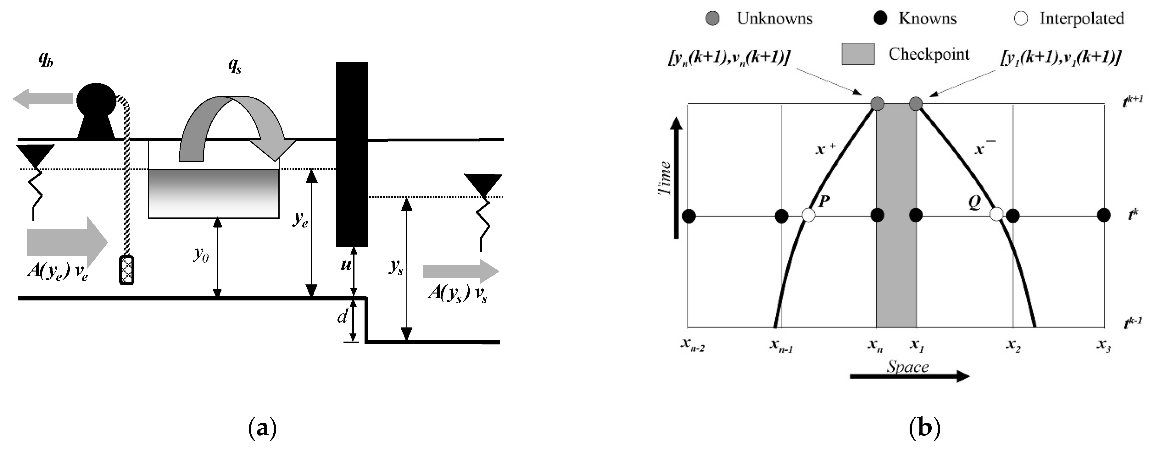
2.1. Free Surface Flow Equations

The equations of Barré de Saint-Venant (1871) [27] describe the free-surface flow in prismatic canals and are the result of the application of the principles of mass conservation and of the quantity of movement in a controlled volume of short length in the direction of flow. A rigorous deduction of these equations for prismatic canals can be found in [27], resulting in the following:

$$\left.\begin{array}{c}{\displaystyle \frac{\mathsf{\partial }y}{\mathsf{\partial }t}}+v{\displaystyle \frac{\mathsf{\partial }y}{\mathsf{\partial }x}}+{\displaystyle \frac{A\left(y\right)}{T\left(y\right)}}{\displaystyle \frac{\mathsf{\partial }v}{\mathsf{\partial }x}}=0\\ {\displaystyle \frac{\mathsf{\partial }v}{\mathsf{\partial }t}}+v{\displaystyle \frac{\mathsf{\partial }v}{\mathsf{\partial }x}}+g{\displaystyle \frac{\mathsf{\partial }y}{\mathsf{\partial }x}}=g\left[S_0-S_f\left(y,v\right)\right]\end{array}\right\}$$

(1)

where x and t are the independent space and time variables, y is the level of the free-surface from canal bottom, v is the average velocity of all particles of a cross section of the flow, A(y) is the area of wet section which depends on the depth, T(y) is the maximum width also dependent on the depth, S₀ is the canal bottom slope, and, finally, S_f (y, v) is the slope friction. These equations cannot be solved analytically, only numerically. Thus, a variety of numerical methods exist, which can be found, among others, in [28].

Usually, Equation (1) is expressed in the classical space and time (x/t) axes, but in the case that we use the so-called characteristic curves, these equations are represented in two curves or characteristics curves, expressed parametrically with x + (t) (downstream curve) and x − (t) (upstream curve), which locally satisfy the two following differential equations:

$$\begin{gathered} \left.\begin{array}{c}{\displaystyle \frac{d{x}^{+}}{dt}}=v+c\left(y\right)\\ {\displaystyle \frac{d{x}^{-}}{dt}}=v-c\left(y\right)\end{array}\right\} \\ \hspace{1em}\hspace{1em}\hspace{1em}\hspace{1em}\hspace{1em}\hspace{1em}\left.\begin{array}{c}{\displaystyle \frac{dv}{dt}}+{\displaystyle \frac{g}{c\left(y\right)}}{\displaystyle \frac{dy}{dt}}=g\left[S_0-S_f\left(y,v\right)\right]\\ {\displaystyle \frac{dv}{dt}}-{\displaystyle \frac{g}{c\left(y\right)}}{\displaystyle \frac{dy}{dt}}=g\left[S_0-S_f\left(y,v\right)\right]\end{array}\right\} \\ c\left(y\right)=\sqrt{{\displaystyle \frac{gA\left(y\right)}{T\left(y\right)}}} \end{gathered}$$

(2)

The nice effect of the transformation of the method of characteristics is that the partial differential Equation (1) becomes an ordinary differential equation system. The difficulty of the method lies in the fact that Equation (1) has to be solved along the characteristic curves or the local axes that are the solution of (2). As the latter is a set of non-linear equations, it obliges us to solve the four equations simultaneously. Fortunately, the curves x + (t) and x − (t) always intersect, although they are not orthogonal, and therefore assure hyperbolicity. The system (2) can be represented in the graph x/t as in Figure 1, where, at the point of intersection R, the four equations are satisfied, and therefore, the four unknowns x, t, y, and v can be found theoretically. This way, if flow conditions at points P and Q are known, the position of point R can be found and integrated numerically, along with the flow conditions.

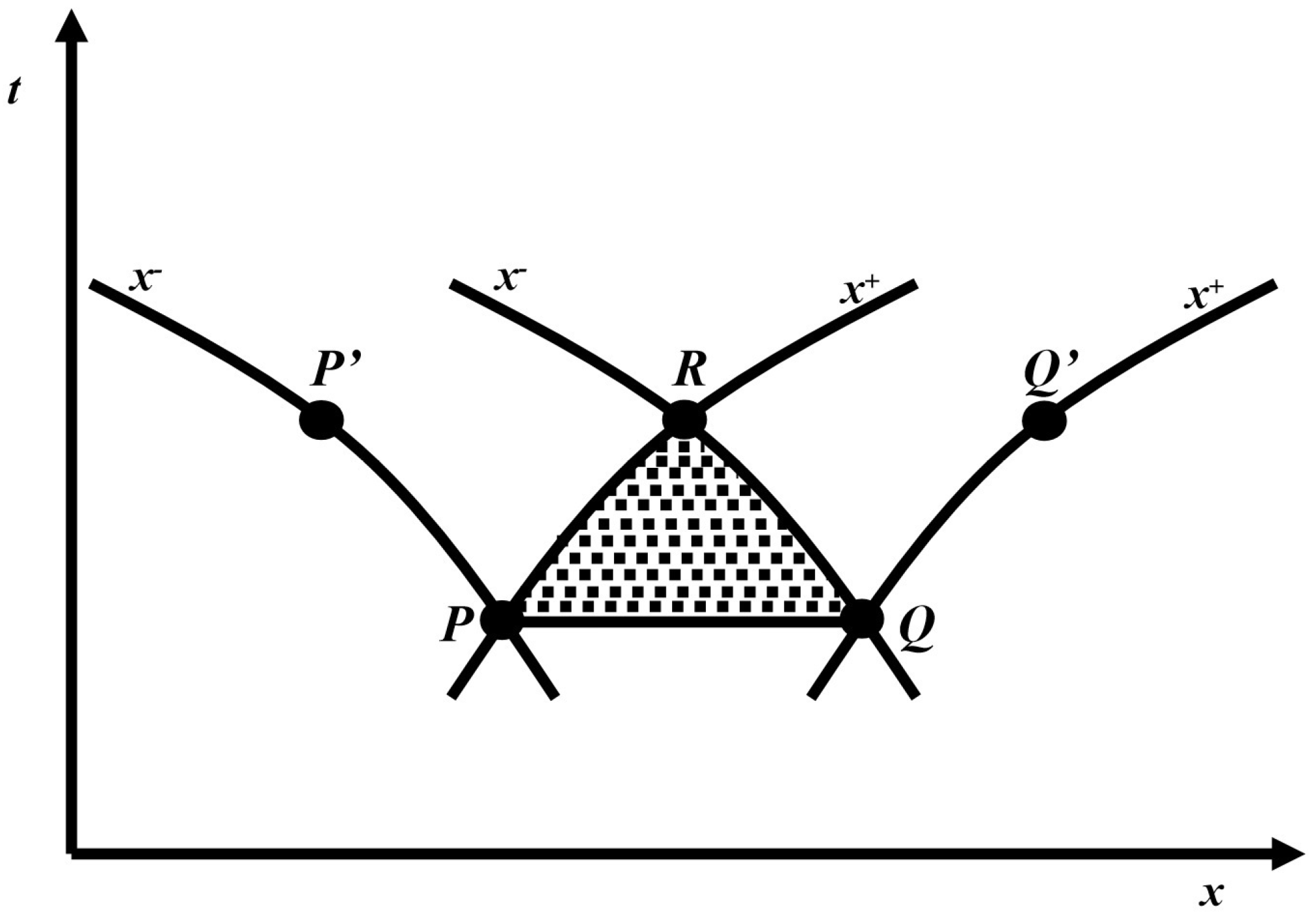
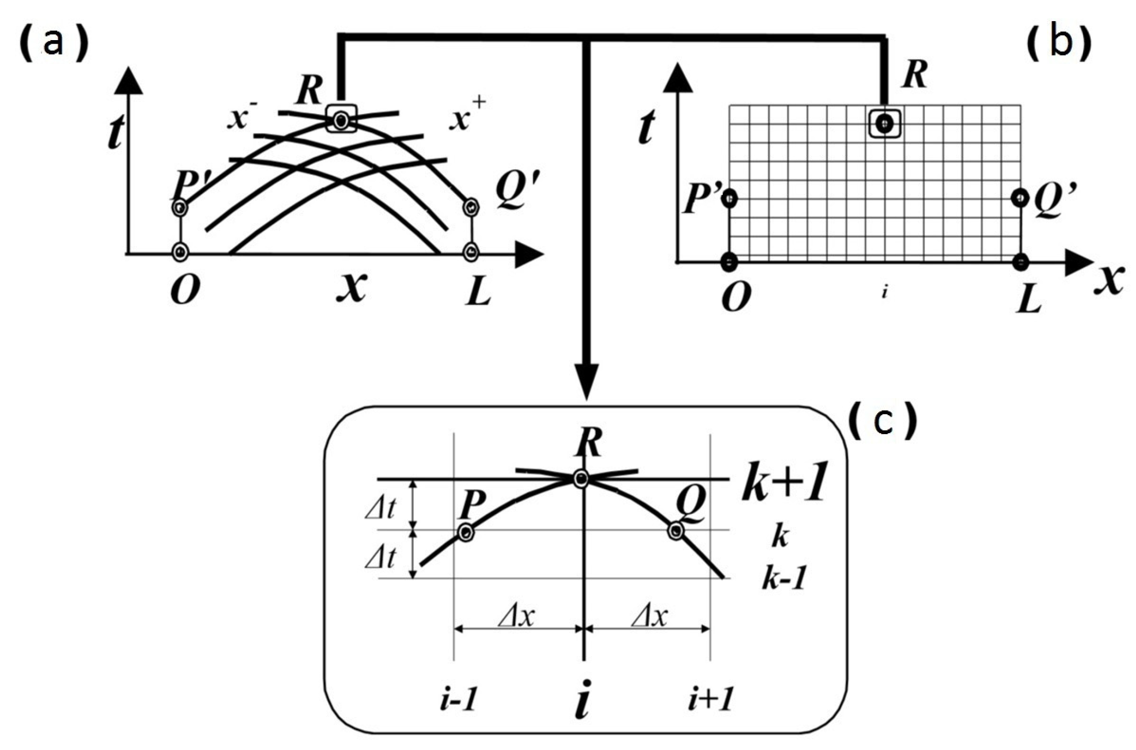
2.2. The Discretization of the Characteristic Equations

As previously mentioned, the system (1) and the equivalent (2) have no known analytical solution, and therefore, the use of numerical techniques has, until present, been compulsory. In this paper, we prefer to use a specific discretization and make the appropriate mathematical developments based on the result of this discretization. In order to have the longest possible integration time period without loss of precision, we adopted a discretization in finite differences of second order, called in [29] as “the method of characteristic curves” applying to a structured grid.

In Figure 2, once can see how by placing the characteristic curves net (Figure 2a) on top of a structured net (Figure 2b), a new scheme is obtained where the variables for points P and Q are interpolated at time step k (Figure 2c). In this way, we can obtain the flow conditions for the fixed-point R at a time step k + 1.

In any case, the irrigation canals are controlled by control structures that are built along the canal (see [30,31,32]). There are many flow control structures in canals, which allow flow modeling according to the specification of the watermaster. The individual study of each of these structures is impossible in this work and does not fall within its aims. However, we present as an example a commonly found structure. It is a checkpoint with a sluicegate, a lateral weir outlet, and a pumping, as seen in Figure 3a. The interaction of this control structure with the flow can be described according to the principles of mass and energy conservation. These principles establish two mathematical relationships between the flow conditions just upstream and downstream of the checkpoint:

$$\left.\begin{array}{c}S\left(y_e\right){\displaystyle \frac{d{y}_e}{dt}}=A\left(y_e\right)v_e-q_b-q_s\left(y_e\right)-A\left(y_s\right)v_s-q_{offtake}\left(y_e\right)\\ \begin{array}{l}{q}_{offtake}(y_e)=C_d{A}_0\sqrt{2g{y}_e}\\ A\left(y_s\right)v_s=k_{c}u\sqrt{y_e-y_s+d}\end{array}\end{array}\right\}$$

(3)

where regarding the first equation; S(y_e) is the horizontal surface of the reception area in the checkpoint; A(y_e)v_e is the incoming flow to checkpoint, defined in terms of water depth and velocity; A(y_s)v_s is the outgoing flow to checkpoint which continues along the canal, described in terms of water depth and velocity; q_b is the pumping offtake, which is predetermined as q_s(y_e) = C_s a_s (y_e − y₀)^3/2 is the outgoing lateral flow via the weir, where C_s is the discharge coefficient, a_s is the width of the lip, and y₀ is the height of the lip measured from the bottom. Considering the second equation, q_offtake is the outgoing offtake orifice flow where C_d is the discharge coefficient, A₀ is the area of the offtake orifice, d is the checkpoint drop, and u is the sluicegate opening. Regarding the last equation, k_c = √2g C_c a_c, where C_c is the discharge coefficient of the sluicegate, a_c is the sluice gate width, and d is the canal step height between pools.

The presence of checkpoints, where water level sensors are deployed, in the middle of a canal leads to the sub-division of this canal into canal pools, in a way that there is a canal pool between two checkpoints, and there is a checkpoint between two pools. The checkpoints are located at and aligned with the positions of the control structures (see Figure 3b). Therefore, y_n^k+1 represents the water level at node n in the section upstream of the control point at time k + 1, that is to say, the incoming water level y_e (Figure 3b).

If discretization is carried out with time, and we rewrite the control structures (3), join them with the characteristics of (2), and then change the nomenclature considering a structured grid, the step-by-step derivation of Equation (4) can be found in [13], so we arrive at the following system of six equations:

$$\begin{array}{c}M={\displaystyle \frac{\mathsf{\partial }\left(f_1,f_2,f_3,f_4,f_5,f_6\right)}{\mathsf{\partial }\left(x_P,y_n^{k+1},v_n^{k+1},y_1^{k+1},v_1^{k+1},x_Q\right)}}\\ N=-{\displaystyle \frac{\mathsf{\partial }\left(f_1,f_2,f_3,f_4,f_5,f_6\right)}{\mathsf{\partial }\left(x_P,y_P,v_P,y_Q,v_Q,x_Q\right)}}\\ L={\left(\begin{array}{cccccc}0& 0& 0& 0& 0& {\displaystyle \frac{\mathsf{\partial }f}{\mathsf{\partial }u}}\end{array}\right)}^T\\ S={\displaystyle \frac{\mathsf{\partial }\left(x_P,y_P,v_P,y_Q,v_Q,x_Q\right)}{\mathsf{\partial }\left(x_P,y_{n-2}^k,v_{n-2}^k,y_{n-1}^k,v_{n-1}^k,y_n^k,v_n^k,y_1^k,v_1^k,y_2^k,v_2^k,y_3^k,v_3^k,x_Q\right)}}\end{array}$$

$$\left.\begin{array}{l}{f}_1\equiv x_n-x_P-{\displaystyle \frac{1}{2}}\Delta t\left[v_n^{k+1}+c_n^{k+1}+v_P+c_P\right]=0\\ f_2\equiv \left(v_n^{k+1}-v_P\right)+{\displaystyle \frac{g}{2}}{\displaystyle \frac{c_n^{k+1}+c_P}{c_n^{k+1}{c}_P}}\left(y_n^{k+1}-y_P\right)-g\Delta t\left({\displaystyle \frac{{S_f}_n^{k+1}+S_{f_P}}{2}}-S_0\right)=0\\ f_3\equiv \left(v_1^{k+1}-v_Q\right)-{\displaystyle \frac{g}{2}}{\displaystyle \frac{c_1^{k+1}+c_Q}{c_1^{k+1}{c}_Q}}\left(y_1^{k+1}-y_Q\right)-g\Delta t\left({\displaystyle \frac{{S_f}_1^{k+1}+S_{f_Q}}{2}}-S_0\right)=0\\ f_4\equiv x_1^{k+1}-x_Q-{\displaystyle \frac{1}{2}}\Delta t\left[v_1^{k+1}-c_1^{k+1}+v_Q-c_Q\right]=0\\ f_5\equiv A\left(y_n^{k+1}\right)v_n^{k+1}-q_b-q_s\left(y_n^{k+1}\right)-A\left(y_1^{k+1}\right)v_1^{k+1}-q_{offtake}(y_n^{k+1})=0\\ f_6\equiv A\left(y_1^{k+1}\right)v_1^{k+1}-k_{c}u\sqrt{y_n^{k+1}-y_1^{k+1}+d}=0\end{array}\right\}$$

(4)

where Δt = t^k+1 − t_P = t^k+1 − t_Q, y_P(x_P) = s(x_P, y_n−2^k, y_n−1^k, y_n^k), y_Q(x_Q) = s(x_Q, y₁^k, y₂^k, y₃^k), v_P(x_P) = s(x_P, v_n−2^k, v_n−1^k, v_n^k), v_Q(x_Q) = s(x_Q, v₁^k, v₂^k, v₃^k), c_n^k+1 = c(y_n^k+1), c₁^k+1 = c(y₁^k+1), Sf_n^k+1 = Sf(y_n^k+1,v_n^k+1), and Sf₁^k+1 = Sf(y₁^k+1,v₁^k+1), where the unknowns are x_P, y_n^k+1, v_n^k+1, y₁^k+1, v₁^k+1, and x_Q. In order to continue with the calculation of the influences of a general parameter φ, it is necessary to assume that this parameter defines the opening of the gate; this is u(φ). Therefore, applying once more the implicit function theorem to (4), with the assumption that y_i−1^k, v_i−1^k, y_i^k, v_i^k, y_i+1^k, v_i+1^k, y_i+1^k+1, and v_i+1^k+1 now depend on a general parameter φ, we can rebuild the equation systems (4) and obtain the next expression:

$$\mathit{M}{\displaystyle \frac{\mathsf{\partial }}{\mathsf{\partial }u\left(\varphi \right)}}\left(\begin{array}{c}{x}_P\\ y_1^{k+1}\\ v_1^{k+1}\\ y_n^{k+1}\\ v_n^{k+1}\\ x_Q\end{array}\right)=\mathit{N}\mathit{S}{\displaystyle \frac{\mathsf{\partial }}{\mathsf{\partial }\varphi }}\left(\begin{array}{c}{y}_{n-2}^k\\ v_{n-2}^k\\ y_{n-1}^k\\ v_{n-1}^k\\ y_n^k\\ v_n^k\\ y_1^k\\ v_1^k\\ y_2^k\\ v_2^k\\ y_3^k\\ v_3^k\end{array}\right)+\mathit{L}{\displaystyle \frac{\mathsf{\partial }u}{\mathsf{\partial }\varphi }}$$

(5)

where the control variable (φ) could be the gate trajectory or pump flow trajectory, that is, another operating variable according to [33,34]. In (6) for the first time, the gate opening u(φ) explicitly appears in the description. Despite the fact that the specific form of this function is still unknown (19), it shows that the influence of the parameter φ on flow conditions at time k + 1 is the sum of the indirect influence of the conditions at instant k and the direct influence of the opening at instant k + 1 through the term ∂u/∂φ_n^k+1.

3. The Linear Hydraulic Model

If all the matrix files (4) of all the state variables (water level “y” and velocity “v”) of any j-gate trajectory (${\displaystyle \frac{\mathsf{\partial }\mathrm{X}}{\mathsf{\partial }\mathrm{U}}}$) are organized and lumped together in a single matrix, the following hydraulic influence matrix, denoted by HIM X(U), is obtained, which defines the behavior of the irrigation canal (y and v) in every section regarding control operation variables (u):

$$\begin{gathered} \hspace{1em}\hspace{1em}\hspace{1em}\hspace{1em}\mathit{H}\mathit{I}{\mathit{M}}_{\mathit{X}}\left(\mathit{U}\right)=\left[\begin{array}{ccccc}{\displaystyle \frac{\mathsf{\partial }{\mathit{X}}_1^{k_F}\left(\mathit{U}\right)}{\mathsf{\partial }{u}_j\left(1\right)}}& \dots & {\displaystyle \frac{\mathsf{\partial }{\mathit{X}}_1^{k_F}\left(\mathit{U}\right)}{\mathsf{\partial }{u}_j\left(K\right)}}& \dots & {\displaystyle \frac{\mathsf{\partial }{\mathit{X}}_1^{k_F}\left(\mathit{U}\right)}{\mathsf{\partial }{u}_j\left(K_F\right)}}\end{array}\right]= \\ \left[\begin{array}{ccccc}{\displaystyle \frac{\mathsf{\partial }{\mathit{x}}^1\left(\mathit{U}\right)}{\mathsf{\partial }{u}_j\left(1\right)}}& & \cdots & & {\displaystyle \frac{\mathsf{\partial }{\mathit{x}}^1\left(\mathit{U}\right)}{\mathsf{\partial }{u}_j\left(K_F\right)}}\\ & \ddots & & ⋰& \\ ⋮& & {\displaystyle \frac{\mathsf{\partial }{\mathit{x}}^k\left(\mathit{U}\right)}{\mathsf{\partial }{u}_j\left(K\right)}}& & ⋮\\ & ⋰& & \ddots & \\ {\displaystyle \frac{\mathsf{\partial }{\mathit{x}}^{k_F}\left(\mathit{U}\right)}{\mathsf{\partial }{u}_j\left(1\right)}}& & \cdots & & {\displaystyle \frac{\mathsf{\partial }{\mathit{x}}^{k_F}\left(\mathit{U}\right)}{\mathsf{\partial }{u}_j\left(K_F\right)}}\end{array}\right] \end{gathered}$$

(6)

The HIM matrix already calculates the water velocity perturbation introduced by gate movements. However, it is not included in this manuscript because common control algorithms typically estimate gate movements based on water levels at checkpoints. Therefore, control algorithms only require water level estimation from models. This is because velocity sensors are usually more expensive and harder to calibrate.

4. Results: Verification of the Linear Hydraulic Model

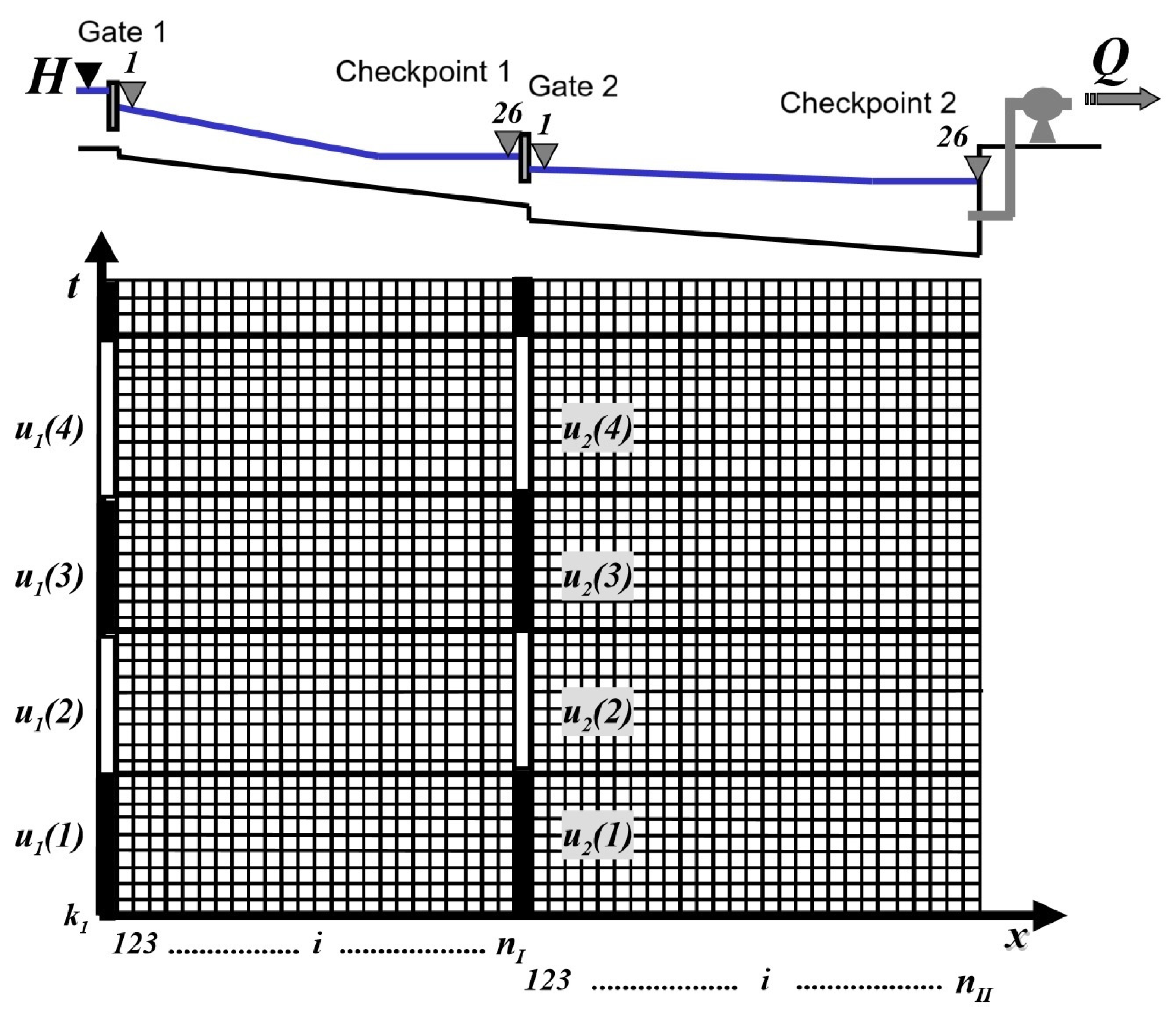
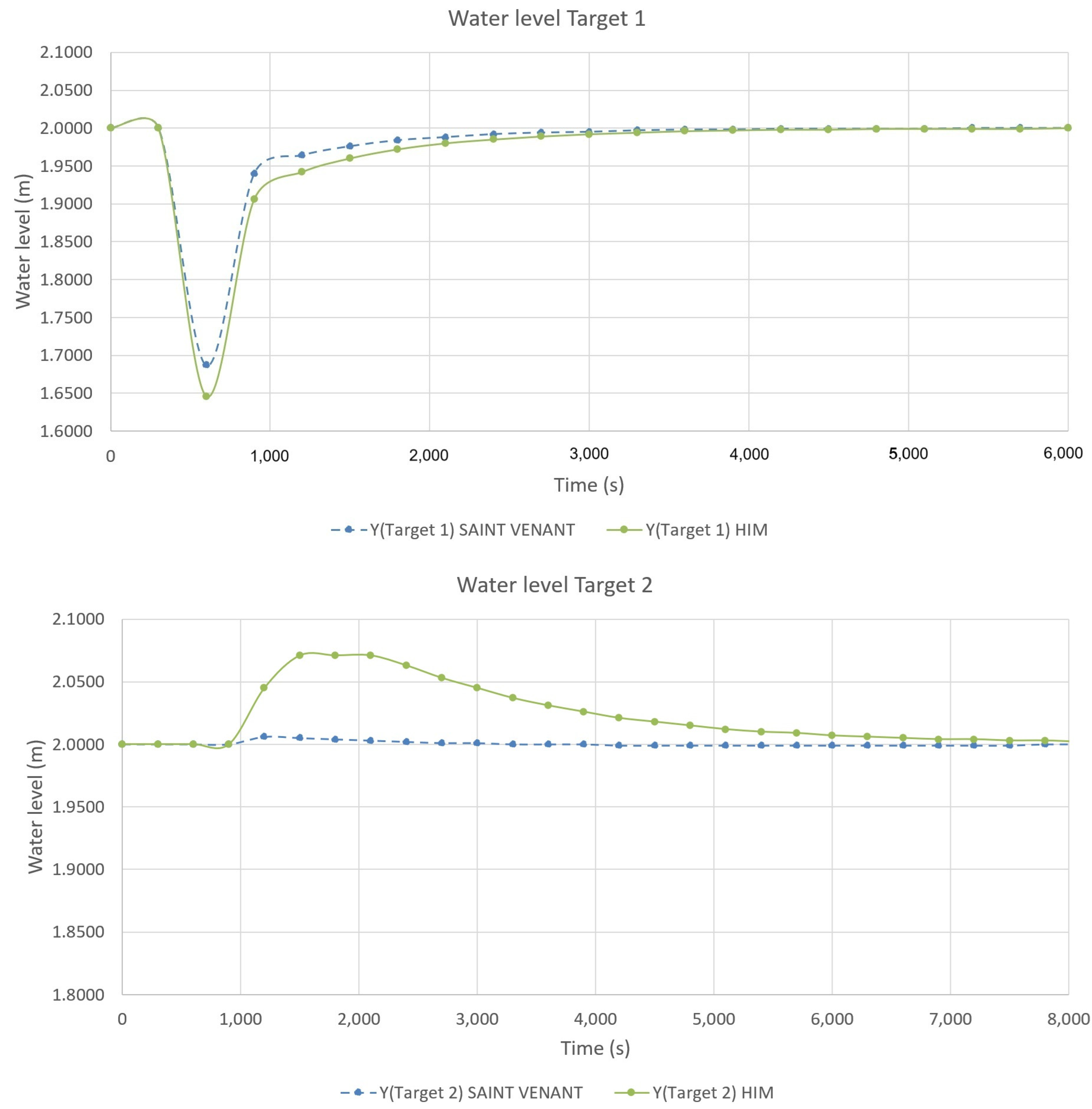
4.1. First Test Case: Irrigation Canal with Two Pools

In order to show the accuracy of our HIM model (linear model) and V.S., a model using the Saint-Venant in its complete form, we evaluated both models taking account a disturbance introduced in a canal in a steady state. This test is explained using an illustrative example. The geometry and features of the irrigation canal (pool length, canal sections, and Manning’s coefficient; see

Table 1. Canal and gates features.

Pool Number (nº)	Pool Length (km)	Bottom Slope (%)	Side Slopes (H:V)	Manning’s Coefficient (n)	Bottom Width (m)	Canal Depth (m)	Gate Discharge Coefficient (-)	Gate Width (m)	Gate Height (m)	Step (m)
I	2.5	0.1	1.5:1	0.025	5	2.5	0.61	5.0	2.5	0.6
II	2.5	0.1	1.5:1	0.025	5	2.5	0.61	5.0	2.5	0.6

) or water control infrastructure features (gate discharge coefficient and gate width; see Table 1) proposed in this test case are based on [35]. A similar canal was also used by different authors, such as [36,37]. The canal geometry adopted in our examples is based on Liu’s example. We can further illustrate the concept of the influence of a gate trajectory variable on the state vector. To do this, consider a numerical example based on a simulation carried out on a 5 km long canal with two pools and three checkpoints (see Figure 4 and Table 1). Each pool is divided into 125 numerical cells, and therefore, there are 126 computational nodes, and n_S = n_I + n_II = 126 + 126 = 252 (cross sections). In this manner, the state vector has 504 components. The boundary conditions are steady: the upstream boundary condition (upstream gate 1) is a constant water level H, and the downstream boundary condition (outlet) is a specified discharge Q (checkpoint 2). Pump station and orifice offtake features are detailed in

Table 2. Pump station/orifice offtake features.

Number of Control Structure or Checkpoint (nº)	Discharge Coef./ Diameter Orifice Offtake (m)	Orifice Offtake Height (m)	Pump Flow (m3/s)
1	2/0.85	0.8	-
2	-	-	5.0

. The initial conditions for this test case are provided in

Table 3. Initial conditions in the canal.

Control Structure	Initial Flow Rate (m3/s)	Control Structure (nº)	Initial Water Level Upstream (m)/ Offtake Orifice Outflow (m3/s)	Control Structure (nº)	Pump Flow Discharge (m3/s)
Gate 1	10.0	Checkpoint 1	2.0/5.0	Checkpoint 2	5.0

.

In these examples, we considered an upstream large reservoir, whose water level H_reservoir is 3 m and constant throughout the test. At the middle of the canal (end of the pool 1), there is a control structure (checkpoint 1) with a gate and an orifice offtake (3) (see Table 2), whose discharge is 5 m³/s.

Here, C_d is the discharge coefficient for an offtake orifice, and A₀ is the area of the offtake orifice, where y is the water level in canal at offtake, and y₀ is the orifice offtake height. At the end of the last pool, there is a control structure with a pump station, which discharges 5 m³/s. The flow through the orifice depends on the level over the orifice and the disturbance. This example starts from an initial steady state (Table 3) with a specific demand delivery constant at the checkpoint 1 (5 m³/s through the orifice offtake) and a constant discharge of 5 m³/s by the pump station at checkpoint 2 (see Figure 4). The disturbance is not introduced initially.

The error between both models (HIM model vs. Saint-Venant in complete form) is estimated using four metrics: the maximum absolute error (I₁), the maximum relative error (I₂), root mean square error (I₃), and Nash–Sutcliffe efficiency (I₄). These indices quantify the deviation of the HIM model from the complete Saint-Venant model at different checkpoints along the canal and at multiple time steps.

(A) Maximum Absolute Error (I₁):

This index represents the maximum absolute difference in water level predictions between both models at any given time step:

$$\mathrm{Maximum} \mathrm{Absolute} \mathrm{error} \mathrm{or} {\mathrm{I}}_1 \left(\mathrm{cm}\right): {max }_{i\in \left[1,n\right]}\left|y_{pij}-y_{ij}\right|$$

(7)

where yp_ij is the water level obtained by the HIM model at time step i at the checkpoint j. y_ij is the water level obtained by the complete Saint-Venant model at time step i at checkpoint j. n is the total number of time steps in the simulation.

(B) Mean Relative Error (I₂):

This index expresses the maximum relative deviation between both models as a percentage of the Saint-Venant model’s water level, across all time steps and checkpoints:

$$\mathrm{Maximum} \mathrm{relative} \mathrm{error} \mathrm{or} {\mathrm{I}}_2 (\%): {\displaystyle \frac{1}{n}}\left({\sum }_{i\ge 1}^n\left({\displaystyle \frac{y_{pij}-y_{ij}}{y_{ij}}}\right)\times 100\right)$$

(8)

where all variables are defined as in the previous equation.

(C) Root Mean Square Error (RMSE):

This indicator quantifies the average magnitude of the error between the water level predictions of the simplified model and the complete Saint-Venant model across all time steps:

$$\mathrm{Root} \mathrm{mean} \mathrm{square} \mathrm{error} \mathrm{or} {\mathrm{I}}_3 \left(\mathrm{cm}\right): \sqrt{{\displaystyle \frac{1}{n}}\left({\sum }_{i=1}^n{\left(y_{pij}-y_{ij}\right)}^2\right)}$$

(9)

where all other variables are defined as above.

(D) Nash–Sutcliffe Efficiency (NSE):

This dimensionless indicator evaluates the predictive performance of the simplified model compared to the variability of the observed data from the Saint-Venant model. Its values range from −∞ to 1:

$$\mathrm{Nash-Sutcliffe} \mathrm{Efficiency} \mathrm{or} {\mathrm{I}}_4 \left(\mathrm{dimensionless}\right): 1-\left({\displaystyle \frac{{\sum }_{i=1}^n{\left(y_{pij}-y_{ij}\right)}^2}{{\sum }_{i=1}^n{\left(y_{ij}-\overline{y_j}\right)}^2}}\right)$$

(10)

where ȳj is the mean of the Saint-Venant model water levels at checkpoint j.

A value of NSE = 1 indicates a perfect match, while NSE ≤ 0 suggests that the model performs worse than simply using the mean of observed values. For this study, the simulation was run with a time step of 300 s over a total duration of 4 h, and the error was evaluated at multiple checkpoints along the canal.

These performance indicators (I₁, I_2, I₃, and I₄) provide a quantitative measure of the accuracy of the HIM model compared to the complete Saint-Venant model, indicating how closely the simplified model approximates the full hydraulic behavior at different locations and times.

The gate movement is set based on a maximum flow disturbance assumed for the system in the context of feedback control in real time. In other words, the criterion was to limit the maximum permissible perturbation for real-time operation according to [36,37,38]. In this context, four different scenarios were proposed, each considering different disturbance values in gate 2 movement: 10% (25 cm), 5% (12.5 cm), 1% (2.5 cm), and 0.5% (1.25 cm). The gate movement conditions are addressed to simulate the impact of disturbances in inflow conditions.

For that reason, it would be useful show the initial and the perturbed discharge under the last sluice gate. The flow discharge by the gate 2 (checkpoint 1) is 5 m³/s in a steady state, and the flow discharge introducing by a gate movement of 10% over the gate height is 5.8 m³/s. In other words, this gate movement involves an incremental discharge of more than 10%. For that reason, introducing a gate-movement higher 10% is not the target of this paper since the HIM simulated lineal model is used in real time, and this sort of disturbance is quite difficult to manage in real time just by feedforward controls. This is why the gate movement disturbance was established to range between 10% and 0.5% (see [39,40]).

The test was performed for four cases; nevertheless, the position of the disturbance in time was always the same (the range step from 300 s to 600 s). The differences between the cases depended on the magnitude of the disturbance. The results obtained using both models are shown in Figure 5.

The results obtained in the four cases are shown in

Table 4. Index error between Linear Hydraulic Model and the Saint-Venant in their complete form.

	I1 (cm)		I2 (%)		I3 (cm)		I4 (Dimensionless)
	Checkpoint 1	Checkpoint 2	Checkpoint 1	Checkpoint 2	Checkpoint 1	Checkpoint 2	Checkpoint 1	Checkpoint 2
Case 1	4.0	6.7	0.17	0.65	0.9	2.41	0.96	−137.2
Case 2	0.9	3.3	0.03	0.32	0.18	1.2	0.99	−73.9
Case 3	0.1	0.7	0	0.06	0.014	0.23	0.999	−35.02
Case 4	0	0.4	0	0.03	0	0.012	1	−12.1

. It can be observed that the error in the first index is significant only in checkpoint 2 of case 1, where the disturbance is 10% above the canal flow. In contrast, the values of the second and third indices are less critical. On the other hand, the fourth index at checkpoint 2 is quite high. This is because the water level at checkpoint 2 remains constant over time, meaning that the average water level equals the observed value throughout the entire period (see, Y (Target 2) Saint-Venant in Figure 5). As a result, when there is a small error between the predicted and the Saint-Venant solution, dividing by a denominator that is close to zero causes the value of the fourth index to increase significantly. Notably, the HIM (linear model) proves to be an excellent tool for understanding flow behavior in real-time scenarios, particularly when flow disturbances are small, and a quick and accurate estimation of the simulated flow state is required.

The computational time for the test cases, considering a PC with an i5 processor and 8 GB of RAM, was significantly different for the two models. For the HIM model, the computational time was 0.01 s, whereas for the full Saint-Venant equations, it was 30 s.

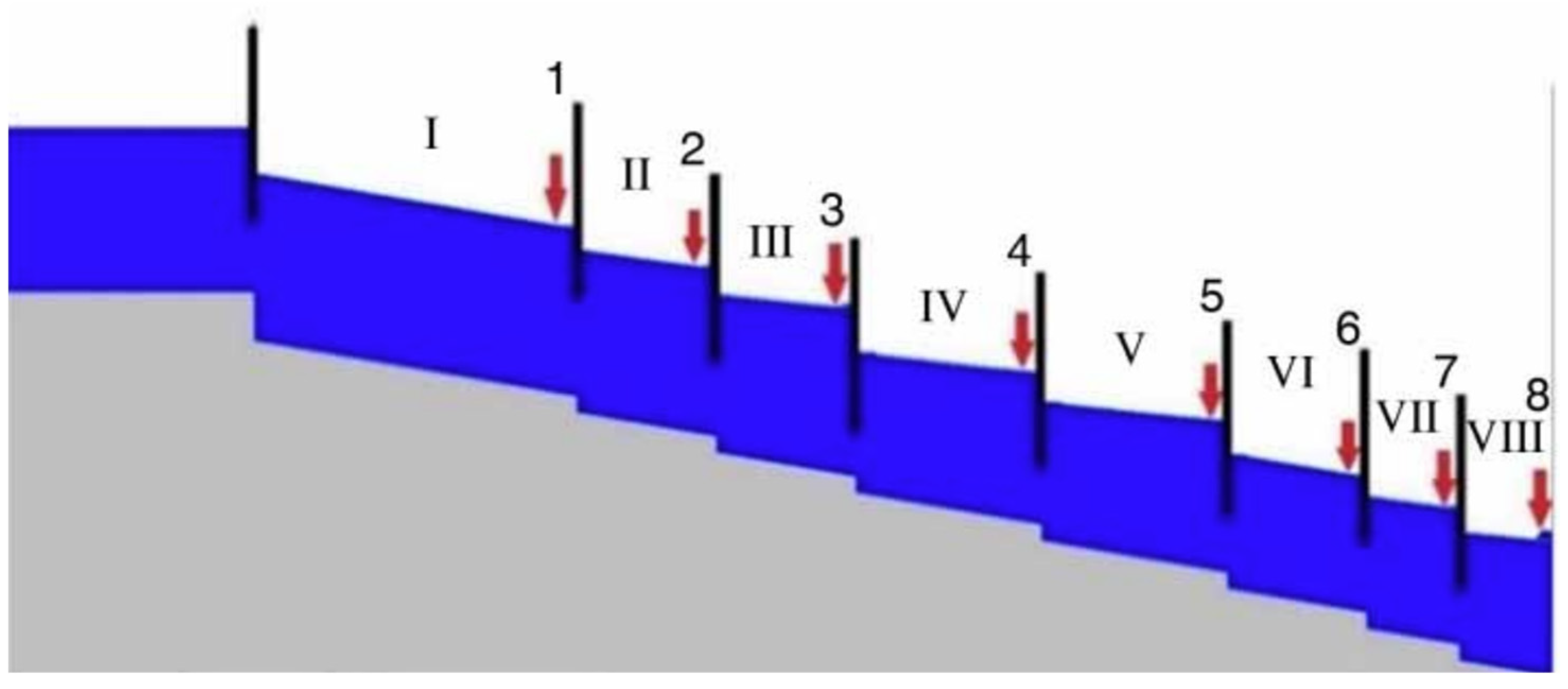
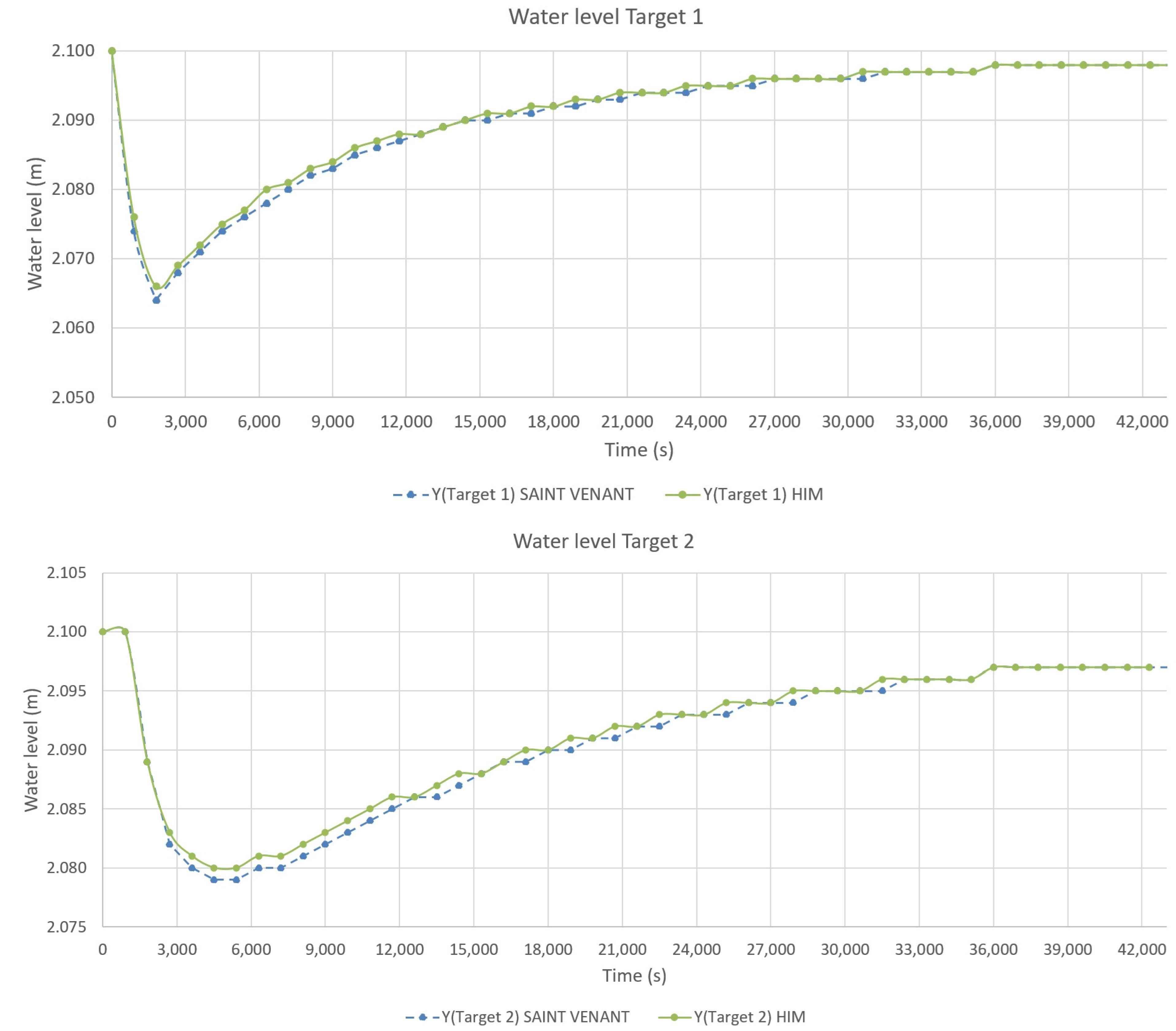
4.2. Second Test Case: ASCE Test Cases

In this numerical example, our goal was to assess the HIM model in a long irrigation canal located in California (USA) within a canal system featuring multiple pools, each experiencing simultaneous flow extractions. To achieve this, we utilized the test cases proposed by the ASCE committee to evaluate control algorithms.

The ASCE Task Committee [41] examines two canals (Maricopa Stanfield and Corning Canal) under various scenarios. In this manuscript, we tested the HIM simulator only on the Corning Canal because this canal exhibits geometric and operational features significantly different from those of the canal tested in the first test cases. The geometry and features of the Corning Canal (pool length, canal sections, and Manning’s coefficient; see

Table 5. Features of Corning Canal pools.

Pool/Checkpoint Number (nº)	Pool Length (km)	Bottom Slope (-)	Side Slopes (H:V)	Manning’s Coefficient (n)	Bottom Width (m)	Canal Depth (m)	Gate Width (m)	Gate Height (m)	Gate Discharge Coefficient (-)	Step (m)	Length from Gate 1 (km)	Orifice Offtake Height (m)	Lateral Spillway Height (m)
0	0	0	0	0	0	0	7	2.3	0.61	0.2	0	-	3
I	7	10−4	1.5:1	0.02	7	2.5	7	2.3	0.61	0.2	7	1.05	2.5
II	3	10−4	1.5:1	0.02	7	2.5	7	2.3	0.61	0.2	10	1.05	2.5
III	3	10−4	1.5:1	0.02	7	2.5	7	2.3	0.61	0.2	13	1.05	2.5
IV	4	10−4	1.5:1	0.02	6	2.3	6	2.1	0.61	0.2	17	0.95	2.3
V	4	10−4	1.5:1	0.02	6	2.3	6	2.1	0.61	0.2	21	0.95	2.3
VI	3	10−4	1.5:1	0.02	5	2.3	5	1.8	0.61	0.2	24	0.85	1.9
VII	2	10−4	1.5:1	0.02	5	1.9	5	1.8	0.61	0.2	26	0.85	1.9
VIII	2	10−4	1.5:1	0.02	5	1.9	-	-	-	-	28	0.85	1.9

) or water control infrastructure features (gate discharge coefficient and gate width; see Table 5 and

Table 6. Corning Canal control structures (Gate 1 is located at the upstream end of the canal).

	Offtake Initial Flow (m3/s)	Check Initial Flow (m3/s)
Heading	-	13.7
1	1.7	12.0
2	1.8	10.2
3	2.7	7.5
4	0.3	7.2
5	0.2	7.0
6	0.8	6.2
7	1.2	5.0
8	2.3	2.7

) proposed in this test case are based on [42]. The geometric properties of the Corning Canal are detailed in Table 5 and illustrated in Figure 6. In each canal, gravity outlet orifices are located at the downstream end of every pool.

The ASCE committee suggests the initial conditions provided in Table 6. In this test, two cases were performed involving a disturbance introduced into the system by the first gate, which changed its position between time steps 0 s and 900 s. In this context, two different scenarios were proposed, each considering different disturbance values in gate 1 movement: 10% (23 cm) and 5% (12.5 cm), according to [39,40].

The results obtained considering performance indicators I₁ and I₂ are the following (

Table 7. Index error between HIM model and the Saint-Venant in their complete form (I₁ and I₂).

	I1 (cm)				I2 (%)
	Checkpoint 1	Checkpoint 2	Checkpoint 3	Checkpoint 4	Checkpoint 1	Checkpoint 2	Checkpoint 3	Checkpoint 4
Case 1	0.2	0.1	0.1	0.1	0.023	0.020	0.018	0.022
Case 2	0.01	0.01	0.02	0.02	0.008	0.01	0.007	0.01

and

Table 8. Index error between HIM model and the Saint-Venant in their complete form (I₃ and I₄).

	I3 (cm)				I4 (Dimensionless)
	Checkpoint 1	Checkpoint 2	Checkpoint 3	Checkpoint 4	Checkpoint 1	Checkpoint 2	Checkpoint 3	Checkpoint 4
Case 1	0.07	0.06	0.006	0.006	0.99	0.98	0.98	0.95
Case 2	0.04	0.04	0.004	0.004	0.99	0.98	0.95	0.90

).

Errors in the first, second, third, and fourth performance indicators were consistently low across all checkpoints, even with a 10% increase in canal flow. In this second test case, all results improved compared to the last test case due to the geometric features of the canal, which help reduce perturbation effects at the checkpoints. A geometry with large cross-sections helps to mitigate the side effects of the water wave by storing the excess water without significantly increasing water levels (see Figure 7).

The computational time for the test cases, considering a PC with an i5 processor and 8 GB of RAM, was quite different for the two models. For the HIM model, the computational time was 0.05 s, whereas for the full Saint-Venant equations, it was 100 s. As the irrigation canal systems became more complex, the computational time for the full Saint Venant models increased, making the HIM matrix increasingly useful for real-time control algorithms. However, it is important to keep in mind that the microprocessors deployed in low-power control algorithms for irrigation gates are not as advanced as the processors found in current laptops.

5. Discussion

5.1. Evaluation and Comparison

The numerical approach presented in this paper employs a second-order finite difference discretization, known as the “method of characteristic curves”, applied to a structured grid. This discretization provides a practical framework for iteratively solving the equations, enabling accurate prediction of flow behavior over extended time periods. Integrating characteristic curves with the structured grid improves numerical precision, especially during flow interpolation at fixed points.

A key contribution of this study is the development of the linear hydraulic model (HIM), which consolidates all state variables, namely water level (y) and velocity (v), into a single matrix. This model is valuable for irrigation control, where real-time water level predictions matter more than accurate velocity measurements due to sensor cost and calibration complexity.

Numerous previous studies [42,43,44,45,46,47,48,49,50,51] have employed high-order models based on the Saint-Venant equations to simulate the behavior of irrigation canals. However, these models involve a high computational cost, particularly in real-time applications. In contrast, the HIM model offers a significant advantage in terms of simulation time, suggesting its feasibility for real-time control contexts without sacrificing accuracy.

Other authors have proposed approximated models, such as the Muskingum model, the integrator delay (ID) model, gray-box models, and black-box models, which have been developed using practical assumptions, fundamental physical principles, empirical observations, and heuristic knowledge [52]. Specifically, the Muskingum–Cunge and integrator delay (ID) models offer high computational efficiency, often requiring computation times comparable to those of the HIM. However, these models make strong assumptions about the flow behavior (e.g., linear storage–discharge relationships), which limits their ability to accurately capture the transient dynamics in open-channel systems, especially near gates or pumps where localized nonlinearities are significant. In contrast, HIM, although linear, preserves a spatially distributed description of the flow, allowing it to better capture the dynamics along the canal while still maintaining a low computational cost, especially in real-time applications.

Similarly, solutions dedicated to real-time simulation, such as those presented in [53,54,55,56,57,58], propose simplified versions of the Saint-Venant equations. While these approaches improve computational speed, they fail to fully capture the complex interactions between various hydraulic variables in irrigation canals. The HIM model, designed to handle free-surface conditions and nonlinear terms in water dynamics, represents a more robust solution for dynamic and complex scenarios.

On the other hand, studies such as [59] compare models based on neural networks, fuzzy systems, and linear systems. In particular, some authors [60] utilized pattern search methods for the online identification of time-varying delays. These models function as black-box approaches, relying on extensive datasets and parallel processing capabilities. However, a major limitation of these methods is their difficulty in learning all possible scenarios and potential states of an irrigation system, leading to “blind spots” where the model’s predictive capability is compromised. In this sense, data-driven models (e.g., black-box or grey-box approaches) can offer good performance and capture nonlinear effects, but their accuracy and generalization capability depend heavily on the quantity, quality, and representativeness of the available training data. Moreover, they often require a substantial amount of data preprocessing, calibration, and validation, which can be a limitation in real-time control where not all scenarios could be preprocessed.

5.2. HIM Limitations

As a linear model, HIM is well suited for scenarios where flow changes are gradual and where the hydraulic system is operating under normal conditions. In particular, it performs reliably when gate movements, pump operations, and downstream demands evolve smoothly, as is typically expected in real-time operational contexts. In contrast, when large and abrupt changes occur, such as sudden gate openings or pump activations, nonlinear effects become more significant, and these events are better addressed through offline planning strategies. Attempting to manage such drastic transitions in real time is inherently complex and may not yield optimal results.

Moreover, even under smooth operational regimes, some level of nonlinearity persists due to the intrinsic behavior of hydraulic structures like gates and pumps. These residual nonlinearities, although moderate, can lead to deviations in the free surface profile that the HIM model does not capture. This divergence becomes more noticeable over time or when structural transitions introduce localized effects not represented in the linear formulation.

This phenomenon is observable in our results. In both case studies, the control targets are located just upstream of gates, where sudden changes in water depth caused by wave propagation are more pronounced. For example, in Figure 5 (target level 1), the highest error between the HIM and the reference model occurs around 600 s, coinciding with the moment of greatest free surface variation, which is not a coincidence, as it coincides with the wave crest arriving at target point 1. On the other hand, when the system stabilizes and these nonlinear effects diminish, both models produce increasingly similar results.

Additionally, the impact of these nonlinearities is not solely dependent on the perturbation introduced (e.g., gate movement or pumping variation) but also on the geometry of the canal and the prevailing hydrodynamic conditions before the disturbance. Therefore, it is important to evaluate in each specific case how and when the HIM model loses accuracy with respect to more comprehensive models, such as the full Saint-Venant equations. This evaluation can help determine when a recalibration or update of the HIM parameters is necessary, based on the actual operating conditions of the system. For instance, if we look at examples 1 and 2, the errors between the HIM model and the complete Saint-Venant equations are greater in the first test case than in the second test case, even though the perturbations are similar in both test cases. This is because, as previously mentioned, the geometry of the canals and the hydrodynamic conditions are very different in both test cases.

5.3. Future Research

While the HIM model demonstrates significant improvements in simulating irrigation canals compared to traditional methods, particularly in real-time control applications, several areas require further investigation in future research:

• The accuracy of the HIM model could be enhanced by refining its boundary condition formulations, particularly for systems with more complex geometries;
• Although the HIM model significantly reduces simulation time, further research is required to evaluate the propagation of small errors, particularly under extreme or highly nonlinear conditions. Recalculating the HIM model should be considered only in cases of discrepancies between the Saint-Venant complete model and the HIM model due to nonlinearity;
• It is expected that future research could improve the HIM model by integrating machine learning techniques to adjust parameters in real time, leading to even faster and more accurate simulations;
• Testing a real-time controller using the HIM model and the complete Saint-Venant equations and analyzing the gate control trajectories in both models and estimating the final control precision would be helpful;
• Future work should also include testing the HIM model in a real-world irrigation system to assess its practical performance and applicability. Despite its promising performance, applying the HIM model to real-world agricultural irrigation systems presents several challenges:
  • Data availability and quality: Accurate simulations require detailed input data, including terrain features, water sources, soil properties, and crop types. Obtaining and maintaining such datasets can be challenging, particularly in remote or less-documented regions. For instance, high-quality topographical and hydrological data might not always be readily available, which can impact the model’s precision. In some cases, satellite imagery or remote sensing technologies may help to mitigate data scarcity, but their accuracy still needs to be validated for specific environments;
  • Calibration and validation: The model must be calibrated and validated using real field data to ensure its reliability in practice. While several methods exist in the literature to address this challenge [61], further empirical studies are necessary to refine the HIM model for use in several environments. Ideally, calibration should involve long-term field studies that capture the dynamic changes in the irrigation system, where coefficients involved in the Saint-Venant equations, such as the Manning coefficient, gate coefficient, or orifice off-take coefficient, may change over time. The lack of such data can hinder the validation process and lead to potential inaccuracies in real-world application;
  • Model adaptability: Agricultural fields are inherently heterogeneous, with varying weather conditions, water availability, and crop growth affecting irrigation dynamics. These factors pose a significant challenge for the HIM model, which must be adaptable to such variability to ensure long-term applicability. The model should integrate real-time seasonal variations in water demand and assess its accuracy in this new environment, which may require additional modifications or extensions;
  • Operational challenges: Besides technical hurdles, implementing the HIM model in real-world irrigation systems also requires addressing practical issues such as the cost and time associated with data collection, model deployment, and continuous monitoring. Operators may face difficulties in integrating the model into existing infrastructure, especially if they lack the necessary technical expertise or resources. Therefore, developing user-friendly interfaces and automated systems for real-time model application and feedback could facilitate the adoption of the model in operational settings.

6. Conclusions

The development of the HIM model was driven by a clear objective: to create a hydraulic modeling framework capable of delivering accurate results while meeting the strict computational demands of real-time control systems. By linearizing the Saint-Venant equations in the unsteady state, the HIM achieves precisely that—a linear yet robust model that significantly reduces computation time without compromising its ability to represent the essential dynamics of open-channel flow. This balance between simplicity and reliability makes the HIM particularly well suited for implementation in irrigation networks, where decisions must be made rapidly and efficiently.

To validate its performance, the HIM model was tested in two contrasting scenarios by introducing perturbations ranging from 10% to 0.5% in gate movement height. The first test was properly conducted, and the predictions made by the HIM were nearly indistinguishable in almost all cases from those of the full Saint-Venant equations. The error metrics confirmed this precision: the maximum absolute error (I₁) ranged between 7 cm and 0.2 cm, while the relative error (I₂) remained between 0.7% and 0.023%. Further supporting the model’s accuracy, the root mean square error (I₃) ranged from 2.4 cm to 0 cm. The Nash–Sutcliffe efficiency (I₄) reached a minimum of 0.96 at checkpoint 1, indicating near-perfect agreement with the reference model. At checkpoint 2, however, the mean water level during the test was very close to the reference level, which caused the denominator of the indicator to approach zero. This led to a situation where even small discrepancies resulted in poor I4 scores, making the indicator unreliable in this specific case.

The second test case focused on the Corning Canal, a benchmark scenario proposed by the ASCE committee to evaluate control algorithms in irrigation systems. Unlike the first test case, this scenario involves a long canal divided into multiple interconnected pools with simultaneous downstream withdrawals an operationally more complex setup that reflects real-world irrigation challenges. The objective was to determine whether the HIM model could accurately capture the hydraulic dynamics of such a system, which includes varied geometries and multiple withdrawal points. To simulate disturbances, flow variations were introduced by adjusting gate 1 during the first 900 s of the simulation. Two scenarios were considered: one with a 10% variation (corresponding to a 23 cm gate displacement) and another with a 5% variation (12.5 cm). Initial conditions and geometric parameters were set according to the ASCE’s standard specifications for the Corning Canal.

The results confirmed that the HIM model maintained high accuracy even under these more demanding conditions. In the 10% disturbance scenario, the maximum absolute error (I₁) at the four monitoring checkpoints ranged from 0.1 to 0.2 cm, while the maximum relative error (I₂) remained between 0.018% and 0.023%. In the 5% disturbance case, these values dropped even further absolute errors ranged from 0.01 to 0.02 cm, and relative errors were below 0.01%. The root mean square error (I₃) remained low throughout: for the 10% disturbance case, values ranged from 0.006 to 0.07 cm, while for the 5% case, they stayed between 0.004 and 0.04 cm. Lastly, the Nash–Sutcliffe efficiency (I₄), which measures how well the model replicates observed data, remained consistently high. In the 10% disturbance scenario, all points scored above 0.95, and in the 5% case, values were still around 0.95.

These findings underscore the robustness of the HIM model in replicating the hydraulic behavior of the Corning Canal, even in the presence of significant flow changes and geometric complexities. While the full Saint-Venant equations require around 30 s per regulation period, the HIM completes the same simulation in just 0.01 s. This computational efficiency, combined with the model’s demonstrated accuracy, makes it a practical and powerful tool for predictive control in irrigation canals.

References

1. UNESCO, 2021. United Nations World Water Development Report 2021: Valuing Water; Facts and Figures. Available online: https://unesdoc.unesco.org/ark:/48223/pf0000375751.locale=en (accessed on 16 December 2024).
2. United Nations, 2024. The Sustainable Development Goals Report 2023, United Nations Department of Economic and Social Affairs. [Online]. Available online: https://unstats.un.org/sdgs/report/2023/The-Sustainable-Development-Goals-Report-2023.pdf (accessed on 10 March 2025).
3. Ingrao, C.; Strippoli, R.; Lagioia, G.; Huisingh, D. Water scarcity in agriculture: An overview of causes, impacts and approaches for reducing the risks. Heliyon 2023, 9, e18507. [Google Scholar] [CrossRef]
4. Mekonnen, M.M.; Hoekstra, A.Y. Four billion people facing severe water scarcity. Sci. Adv. 2016, 2, e1500323. [Google Scholar] [CrossRef] [PubMed] [PubMed Central]
5. Jägermeyr, J.; Pastor, A.; Biemans, H.; Gerten, D. Reconciling irrigated food production with environmental flows for Sustainable Development Goals implementation. Nat. Commun. 2017, 8, 15900. [Google Scholar] [CrossRef]
6. Qin, J.; Duan, W.; Zou, S.; Chen, Y.; Huang, W.; Rosa, L. Global energy use and carbon emissions from irrigated agriculture. Nat. Commun. 2024, 15, 3084. [Google Scholar] [CrossRef] [PubMed] [PubMed Central]
7. Tzanakakis, V.A.; Paranychianakis, N.V.; Angelakis, A.N. Water Supply and Water Scarcity. Water 2020, 12, 2347. [Google Scholar] [CrossRef]
8. Dinar, A.; Tieu, A.; Huynh, H. Water scarcity impacts on global food production. Glob. Food Secur. 2019, 23, 212–226. [Google Scholar] [CrossRef]
9. Aiswarya, L.; Siddharam; Gaddikeri, V.; Jatav, M.S.; Dimple; Rajput, J. Canal Automation and Management System to Improve Water Use Efficiency. In Recent Advancements in Sustainable Agricultural Practices; Yasheshwar, Mishra, A.K., Kumar, M., Eds.; Springer: Singapore, 2024. [Google Scholar] [CrossRef]
10. Kadpan, W.R.; Mustafa, F.F.; Kadhim, H.T. A review of control automatically water irrigation canal using multi controllers and sensors. J. Eur. Des Systèmes Automatisés 2024, 57, 717–727. [Google Scholar] [CrossRef]
11. Abioye, E.A.; Abidin, M.S.Z.; Aman, M.N.; Mahmud, M.S.A.; Buyamin, S. A model predictive controller for precision irrigation using discrete lagurre networks. Comput. Electron. Agric. 2021, 181, 105953. [Google Scholar] [CrossRef]
12. Soler, J.; Gómez, M.; Rodellar, J. A control tool for irrigation canals with scheduled demands. J. Hydraul. Res. 2008, 46, 152–167. [Google Scholar] [CrossRef]
13. Bonet Gil, E. Experimental Design and Verification of a Centralized Controller for Irrigation Canals. Tesi Doctoral, UPC, Escola Tècnica Superior d'Enginyers de Camins, Canals i Ports de Barcelona, 2015. Available online: http://hdl.handle.net/2117/95654 (accessed on 3 March 2025). [CrossRef]
14. Liao, W.; Guan, G.; Tian, X. Exploring Explicit Delay Time for Volume Compensation in Feedforward Control of Canal Systems. Water 2019, 11, 1080. [Google Scholar] [CrossRef]
15. Huang, M.; Tian, M.; Liu, Y.; Zhang, Y.; Zhou, J. Parameter optimization of PID controller for water and fertilizer control system based on partial attraction adaptive firefly algorithm. Sci. Rep. 2022, 12, 12182. [Google Scholar] [CrossRef]
16. Chen, P.C.; Luo, Y.; Peng, Y.B.; Chen, Y.Q. Optimal robust fractional order (PID)-D-lambda controller synthesis for first order plus time delay systems. ISA Trans. 2021, 114, 136–149. [Google Scholar] [CrossRef]
17. Arauz, T.; Maestre, J.M.; Tian, X.; Guan, G. Design of PI controllers for irrigation canals based on linear matrix inequalities. Water 2020, 12, 855. [Google Scholar] [CrossRef]
18. Malaterre, P.O. PILOTE: Optimal control of irrigation canals. In Proceedings of the First International Conference on Water Resources Engineering, Irrigation and Drainage, San Antonio, TX, USA, 14–18 August 1995. [Google Scholar]
19. Malaterre, P.O. Modelisation, Analysis and LQR Optimal Control of an Irrigation Canal. Ph.D. Thesis, LAAS-CNRS-ENGREF-Cemagref, Etude EEE nº14. FR. École Nationale du Génie Rural, des Eaux et des Forêts, Paris, France, 1994. [Google Scholar]
20. Durdu, O.F. Optimal control of irrigation canals using recurrent dynamic neural network (RDNN). Crit. Transit. Water Environ. Resour. Manag. 2012, 1–12. [Google Scholar] [CrossRef]
21. Heyden, M.; Pates, R.; Rantzer, A. A Structured Optimal Controller for Irrigation Networks. In Proceedings of the 2022 European Control Conference (ECC), London, UK, 11–14 July 2022; IEEE: Piscataway, NJ, USA, 2022. [Google Scholar]
22. Gómez, M.; Rodellar, J.; Mantecón, J. Predicitve control method for decentralized operation of irrigation canals. Appl. Math. Model. J. 2001, 26, 1039–1056. [Google Scholar] [CrossRef]
23. Rodellar, J.; Gómez, M.; Martín, J.P. Stable Predictive Control of Open-Channel Flow. J. Irrig. Drain. Eng. 1989, 115, 701–713. [Google Scholar] [CrossRef]
24. Gejadze, I.; Malaterre, P.O. Discharge estimation under uncertainty using variational methods with application to the full Saint-Venant hydraulic network model. Int. J. Numer. Meth. Fluids 2016, 83, 405–430. [Google Scholar] [CrossRef]
25. Hernández López, Y.; Rivas-Pérez, R.; Feliu-Batlle, V. IMC-PID controller with fractional-order filter for a main irrigation canal section. Rev. Científica De Ing. Electrónica Automática Comun. 2021, 42, 74–88. [Google Scholar]
26. Alla, A.; Berardi, M.; Saluzzi, L. A feedback control strategy for optimizing irrigation in a Richards’ Equation framework. arXiv 2024, arXiv:2407.06477. [Google Scholar]
27. Walker, W.R.; Skogerboe, G.V. Surface Irrigation: Theory and Practice; Prentice-Hall, Inc.: Englewood Cliffs, NJ, USA, 1987. [Google Scholar]
28. Wylie, E.B. Control of transient free-surface flow. J. Hydr. Div. (ASCE) 1969, 40, 347–361. [Google Scholar] [CrossRef]
29. Gómez, M. Contribución al Estudio del Movimiento Variable en Lámina Libre, en las Redes de Alcantarillado. Ph.D. Thesis, UPC, Barcelona, Spain, 1988. [Google Scholar]
30. Ames, W.F. Numerical Methods for Partial Differential Equations; Academic Press Inc.: Orlando, FL, USA, 1977. [Google Scholar]
31. Ducheteau, P.; Zachmann, D.W. Ecuaciones Diferenciales Parciales; McGraw-Hill Interamericana de México: Ciudad de México, Mexico, 1988. [Google Scholar]
32. Crandall, S.H. Engineering Analysis—A Survey of Numercial Procedures; Wiley (Interescience): New York, NY, USA, 1956. [Google Scholar]
33. Bonet, E. Experimental Design and Verification of a Centralize Controller for Irrigation Canals. Ph.D. Thesis, UPC, Technical University of Catalonia, Barcelona, Spain, 2015. [Google Scholar]
34. Soler, J.; Gómez, M.; Bonet, E. Canal monitoring algorithm. J. Irrig. Drain. Eng. 2016, 142, 04015058. [Google Scholar] [CrossRef]
35. Bautista, E.; Clemmens, A.J.; Strelkoff, T. Comparison of numerical procedures for gate stroking. J. Irrig. Drain. Eng. ASCE 1997, 113, 129–136. [Google Scholar] [CrossRef]
36. Liu, F.; Feyen, J.; Berlamont, J. Computation method for regulating unsteady flow in open channels. J. Irrig. Drain. Eng. ASCE 1992, 118, 674–689. [Google Scholar] [CrossRef]
37. Chevereau, G. Contribution à L’étude de la Régulation dans les Systems Hydrauliques à Surface Libre. Ph.D. Thesis, de l’Institut National Polytechnic de Grenoble, Grenoble, France, 1991. [Google Scholar]
38. Litrico, X.; Fromion, V. Tuning of Robust Distant Downstream PI Controllers for an Irrigation Canal Pool. I: Theory. J. Irrig. Drain. Eng. 2006, 132, 359–368. [Google Scholar] [CrossRef]
39. Aguilar, J.V.; Langarita, P.; Rodellar, J.; Linares, L.; Horváth, K. Predictive control of irrigation canals robust design and real-time implementation. Water Resour Manag. 2016, 30, 3829–3843. [Google Scholar] [CrossRef]
40. Wu, Y.; Li, L.; Liu, Z.; Chen, X.; Huang, H. Real-Time Control of the Middle Route of South-to-North Water Diversion Project. Water 2021, 13, 97. [Google Scholar] [CrossRef]
41. Clemmens, A.J.; Kacerek, T.F.; Grawitz, B.; Schuurmans, W. Test Cases for Canal Control Algorithms. J. Irri. Drain. ASCE 1998, 124, 23–30. [Google Scholar] [CrossRef]
42. Durdu, O. Regulation of irrigation canals using a two-stage linear quadratic reliable control. Turk. J. Agric. For. 2004, 28, 111–120. [Google Scholar]
43. Durdu, O. Control of transient flow in irrigation canals using Lyapunov fuzzy filter-based gaussian regulator. Int. J. Numer. Methods Fluids 2006, 50, 491–509. [Google Scholar] [CrossRef]
44. Feng, X.; Wang, K. Stability analysis on automatic control methods of open canal. Wuhan Univ. J. Nat. Sci. 2011, 16, 325–331. [Google Scholar] [CrossRef]
45. Garcia, A.; Hubbard, M.; De Vries, J. Open channel transient flow control by discrete time LQR methods. Automatica 1992, 28, 255–264. [Google Scholar] [CrossRef]
46. Bonet, E.; Gómez, M.; Yubero, M.; Fernández-Francos, J. GoRoSoBo: An overall control diagram to improve the efficiency of water transport systems in real time. J. Hydroinformatics 2017, 19, 364–384. [Google Scholar] [CrossRef]
47. Breckpot, M.; Agudelo, O.; Moor, B.; De Moor, B. Flood control with model predictive control for river systems with water reservoirs. J. Irrig. Drain. Eng. 2013, 139, 532–541. [Google Scholar] [CrossRef]
48. Cen, L.; Wu, Z.; Chen, X.; Zou, Y.; Zhang, S. On modeling and constrained model predictive control of open irrigation canals. J. Control. Sci. Eng. 2017, 2017, 6257074. [Google Scholar] [CrossRef]
49. Lacasta, A.; Morales-Hernández, M.; Brufau, P.; García-Navarro, P. Application of an adjoint-based optimization procedure for the optimal control of internal boundary conditions in the shallow water equations. J. Hydraul. Res. 2018, 56, 111–123. [Google Scholar] [CrossRef]
50. Shang, Y.; Liu, R.; Li, T.; Zhang, C.; Wang, G. Transient flow control for an artificial open channel based on finite difference method. Sci. China Technol. Sci. 2011, 54, 781–792. [Google Scholar] [CrossRef]
51. Xu, M.; Negenborn, R.; van Overloop, P.; van de Giesen, N. De saint-venant equations-based model assessment in model predictive control of open channel flow. Adv. Water Resour. 2012, 49, 37–45. [Google Scholar] [CrossRef]
52. McCarthy, G. The Unit Hydrograph and Flood Routing; U.S. Engineer Office: Providence, RI, USA, 1939. [Google Scholar]
53. Koenig, D.; Bedjaoui, N.; Litrico, X. Unknown input observers design for time-delay systems application to an open-channel. In Proceedings of the 44th IEEE conference on decision and control, Seville, Spain, 15 December 2005; pp. 5794–5799. [Google Scholar]
54. Litrico, X.; Fromion, V. Modeling and Control of Hydrosystems; Springer: London, UK, 2009; pp. 1–409. [Google Scholar]
55. Horváth, K.; Galvis, E.; Rodellar, J.; Valentín, M. Experimental comparison of canal models for control purposes using simulation and laboratory experiments. J. Hydroinformatics 2014, 16, 1390–1408. [Google Scholar] [CrossRef]
56. Puig, V.; Ocampo-Martinez, C.; Negenborn, R. Transport of water versus transport over water: Model predictive control for combined water supply and navigability/sustainability in river systems. In Transport of Water Versus Transport Over Water; Ocampo-Martinez, C., Negenborn, R.R., Eds.; Springer International Publishing: Berlin/Heidelberg, Germany, 2015; pp. 13–32. [Google Scholar]
57. Van Overloop, P.; Horvath, K.; Ekin, B. Model predictive control based on an integrator resonance model applied to an open water channel. Control. Eng. Pract. 2014, 27, 54–60. [Google Scholar] [CrossRef]
58. Zheng, Z.; Wang, Z.; Zhao, J.; Zheng, H. Constrained model predictive control algorithm for cascaded irrigation canals. J. Irrig. Drain. Eng. 2019, 145, 04019009. [Google Scholar] [CrossRef]
59. Tavares, I.; Borges, J.; Mendes, M.; Botto, M. Assessment of data-driven modeling strategies for water delivery canals. Neural Comput. Appl. 2013, 23, 625–633. [Google Scholar] [CrossRef]
60. Herrera, J.; Ibeas, A.; De La Sen, M. Identification and control of integrative MIMO systems using pattern search algorithms: An application to irrigation channels. Eng. Appl. Artif. Intell. 2013, 26, 334–346. [Google Scholar] [CrossRef]
61. Bonet, E.; Russo, B.; González, R.; Yubero, M.T.; Gómez, M.; Sánchez-Juny, M. The FC Algorithm to Estimate the Manning’s Roughness Coefficients of Irrigation Canals. Agriculture 2023, 13, 1351. [Google Scholar] [CrossRef]
Figure 1. The domain of dependence of point R with respect to water perturbations (y, v) originating from points P or Q.
Water 17 01368 g001
Figure 2. The steps for the interpolation onto a structured grid.
Water 17 01368 g002
Figure 3. (a) Diagram of a checkpoint with gate, lateral weir, and pumping. (b) Graph with discretization of checkpoints.
Water 17 01368 g003
Figure 4. Sketch of the numerical example based on canal with two pools and two checkpoints. In the superior part, we can see a water depth profile corresponding to a backwater curve with H as the upstream water level and Q as the downstream discharge.
Water 17 01368 g004
Figure 5. Water level vs. time comparing HIM simulation and complete Saint-Venant equations in the first test case with a 10% gate movement disturbance at checkpoints 1 and 2 in the first test case.
Water 17 01368 g005
Figure 6. Corning Canal profile. The red lines mark the position of checkpoints. The first pool is number I, and the first checkpoint is number 1.
Water 17 01368 g006
Figure 7. Water level vs. time comparing HIM simulation and complete Saint-Venant equations in the first test case with a 10% gate movement disturbance at checkpoints 1 and 2 in second test cases.
Water 17 01368 g007