Accuracy Evaluation of a Wave Monitoring System by Testing the Hydraulic Performance of Portable Low-Cost Buoys

Abstract

Lakes are complex ecosystems affected by various anthropogenic influences, including vessel-induced waves. Detecting these waves by a micro-electro-mechanical system (MEMS)-based inertial measurement unit (IMU) equipped on a buoy-based monitoring system can help assess their impacts and support developing sustainable water ecosystem management. This study evaluated and optimized the measurement accuracy of a wave-monitoring system designed to detect waves generated by recreational vessels on lakes. In laboratory tests, we analyzed and, separately, compared the hydraulic behavior of different buoy configurations and assessed the IMU integration in field test campaigns. Results showed that all tested buoys exhibited a mean average absolute deviation (AAD) of less than 20 mm, while the IMU integration achieved an overall AAD of $1.9$ mm. For small waves, characterized by wave heights < 50 mm, the IMU’s AAD corresponds to the buoy’s AAD. However, for larger waves, the buoy’s AAD often significantly exceeds that of the IMU, indicating that the hydraulic performance of the buoy limits measurement accuracy in case of greater waves. The best-performing buoy configuration in laboratory tests achieved a measurement accuracy (mean AAD) below 10 mm (or $10\%$ of wave height), confirming the suitability of the developed wave buoys for a vessel-induced wave-monitoring system on lakes.

1. Introduction

Freshwater ecosystems offer a wide range of ecosystem services and contribute significantly to human well-being [1]. Among these services, recreational activities like boating cover a major cultural aspect. However, these recreational boating activities can impact lake ecosystems: wave energy generated by boat traffic can contribute significantly to total wave energy and cause shoreline erosion, sediment resuspension [2,3], and the disturbance of aquatic habitats, thereby altering the ecological balance of these [4,5]. Despite these potential impacts, a comprehensive assessment of the ecological effects of waves generated by recreational boats remains limited due to an incomplete understanding of typical wave-induced processes in these systems. In addition, the distinction between wind-induced and vessel-induced waves is not comprehensively solved yet, making it difficult to accurately identify the source of these processes. This highlights the need for developing improved methods for monitoring and analyzing high-frequency wave activity. In particular, the provision of high-resolution data on wave patterns in recreational lakes is essential for the sustainable management of water ecosystems. Since the impact of waves caused by boating activities depends on the frequency of passing boats, boat and driving characteristics [6,7] as well as the bathymetry of the shore [8], it is evident that monitoring wave exposure at a single point is insufficient, reinforcing the need for more comprehensive spatial approaches. To address this, we developed a portable monitoring system designed to assess multiple shoreline sections, specifically adapted to the typical wave characteristics induced by recreational boats. Those waves are characterized by wave heights (H) ranging from $0.04$ m to $0.28$ m [7] and periods (T) between 1–3 s [3,9] in deep water. Those characteristics are crucial criteria for a suitable wave-monitoring system detecting recreation waves. To record waves between 0.04–0.28 m on a certain detail level, we expect a measurement accuracy of 1 cm and a recordable frequency range of 1–0.3 Hz for our monitoring system. Traditionally, wave monitoring has relied on buoys designed for maritime applications, where oceanic wave conditions differ substantially from those in lakes. These conventional wave buoys, while highly sophisticated, often come with high costs and are optimized for open-sea conditions, making them less suitable for small-scale, cost-sensitive lake monitoring. The financial investment required for a comprehensive monitoring system such as the one tested in this study, which incorporates eight wave-buoys, is often substantial and can act as a limiting factor for ecological monitoring projects. While there have been advancements in low-cost wave-monitoring technologies [10,11,12,13,14], these solutions typically remain tailored for oceanic use, featuring large dimensions that hinder their portability and applicability for monitoring varying shore sections. Those large dimensions of the buoys often impede the detection of waves with periods lower than 1.7–2.5 s [15], which is in the range of our wave spectrum of interest, the typical wave characteristics induced by recreational boats in deep water. Furthermore, measurement accuracies of those open-sea buoys are difficult to transfer, since calibration data is based on large wave heights (e.g., in following references [16,17] with significant wave heights of 0.4–1.8 m), which overtops substantially the waves of our interest (0.04–0.28 m). There are precise products with accuracies of 1.4 cm [18], 2.57 cm [19], 3.4 cm [13], whereas deviations up to 6 cm [20] or 10 cm [16] would not allow evaluations of the recreational boat-waves of our interest. Recent innovations, such as those by the authors of [15,21,22], demonstrate promising developments but still fall short of meeting the specific requirements for effectively monitoring boat-induced waves in lakes. It was shown that micro-electro-mechanical systems (MEMS)-based inertial measurement units (IMUs) are suitable for detecting short-frequency waves [15,23], in which we are especially interested regarding boat-induced waves. 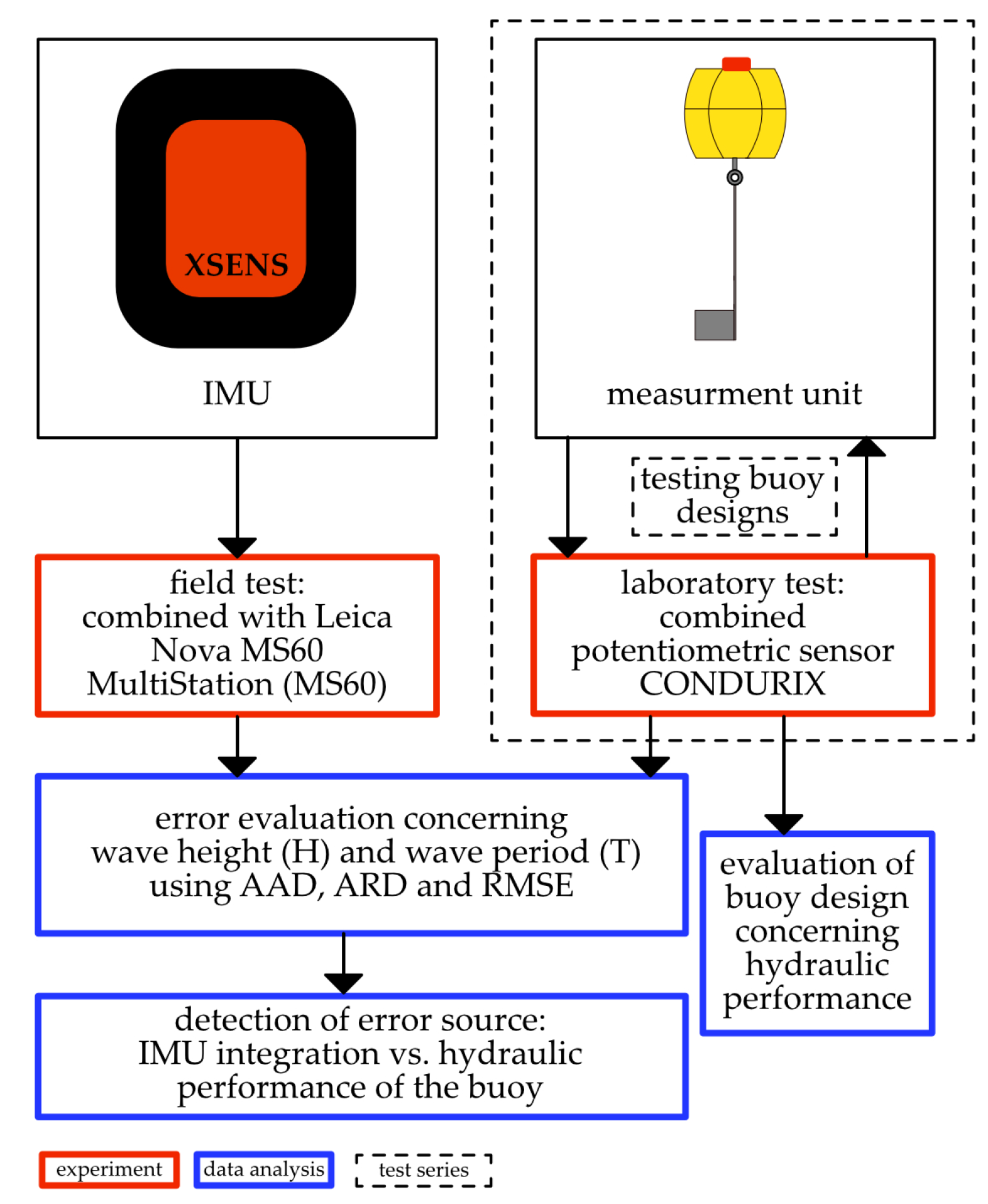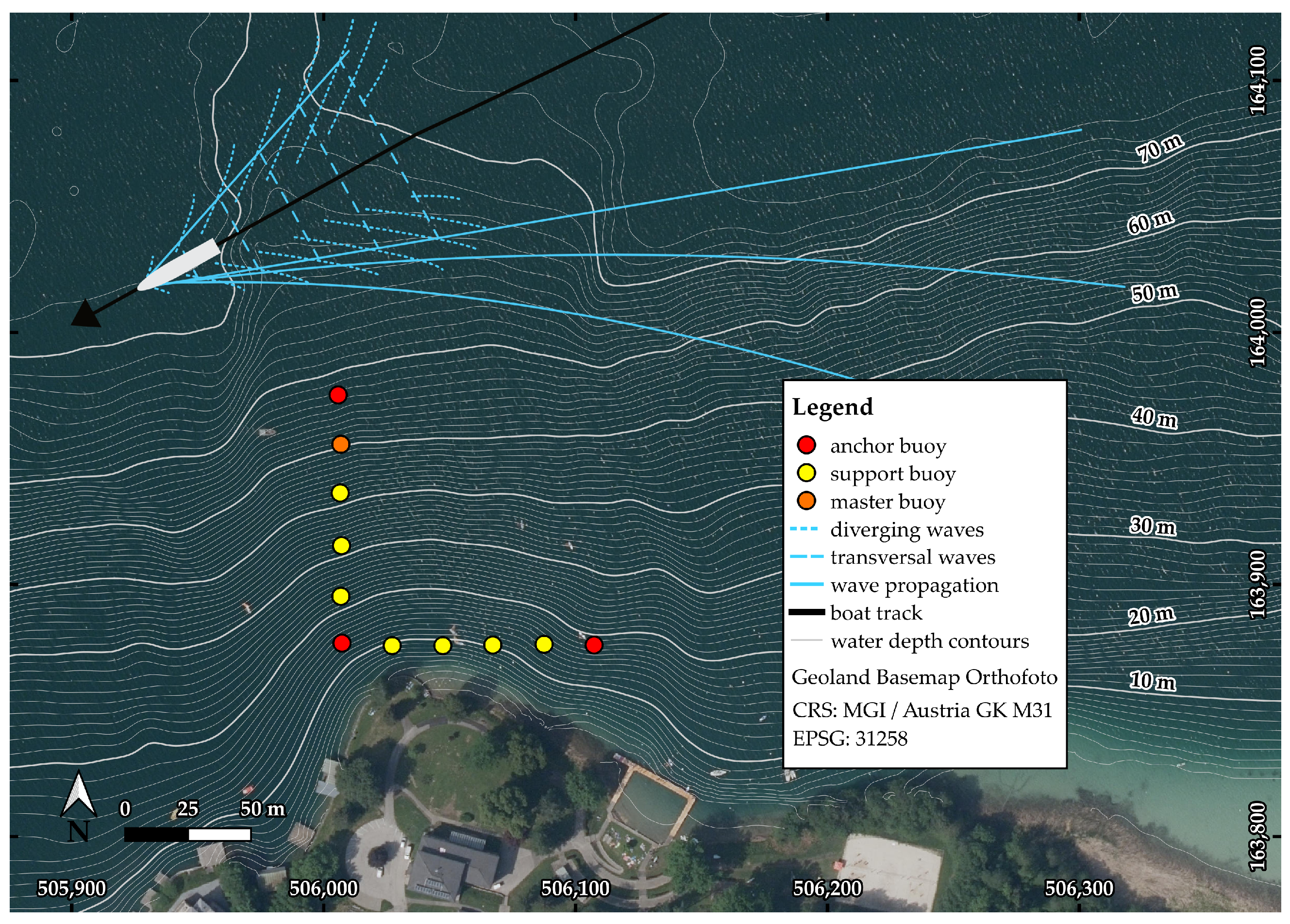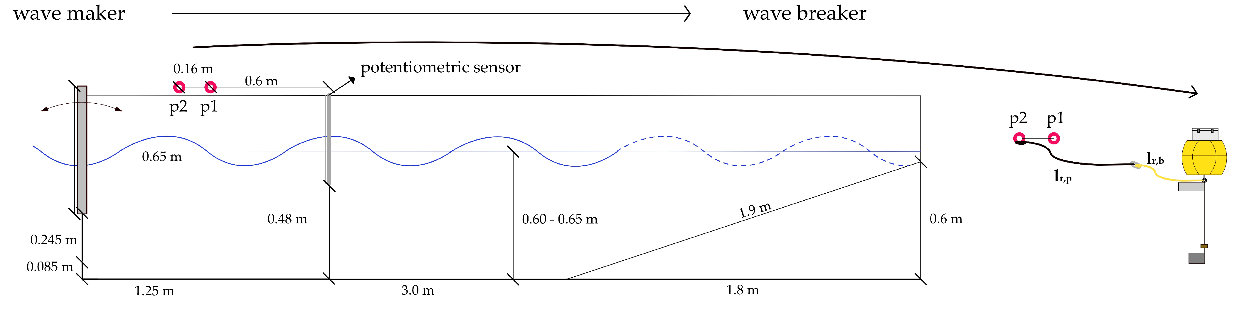Combining this IMU technology with buoys, we extended a cost-effective buoy system for monitoring boat-induced waves in lake environments [23], prioritizing affordability without sacrificing the accuracy of wave measurements. The given system architecture and test setup are based on the system described in Mascher and Berglez [23]. The monitoring system consists of individual measurement units, which can be distinguished between a master buoy unit and a support buoy unit. Both types of buoys are attached to a connecting rope between the anchor buoys at a fixed position using a carabiner-equipped rope measuring 40 cm in length, allowing each buoy a free-floating radius of 40 cm. Each monitoring system is equipped with one master buoy. The support buoys are equipped with a single MEMS-based Xsens DOT IMU (by Movella®, Henderson, NV, USA) sensor mounted on top. In contrast to the system developed by Mascher and Berglez [23], the master buoy is significantly enhanced: in addition to the Leica GRZ101 360 degree Mini Reflector and a Xsens DOT, it integrates a single-board computer, a Global Navigation Satellite Systems (GNSS) receiver, and a SparkFun GPS-RTK Dead Reckoning module. These components enable continuous GNSS data collection, primarily serving as a precise time reference for synchronized data acquisition in this study. A key novelty of the system lies in the integration of Inertial Navigation System (INS) and GNSS data, which not only enables accurate measurements of wave heights through inertial sensors but also allows for compensation of horizontal buoy drift by incorporating previously unavailable attitude information into the processing framework. Drift correction can be performed in near real-time using the publicly available Galileo High Accuracy Service (HAS), offering the potential for significantly improved accuracy [24]. Since the waves of interest have small amplitudes and periods, the requirements for measurement accuracy are stringent and are within 1 cm concerning wave height. Previous investigations of the tested wave-monitoring system have achieved an accuracy of the IMU integration in terms of averaged root mean square error (RMSE) between $1.5$ and $4.3$ cm [23]. 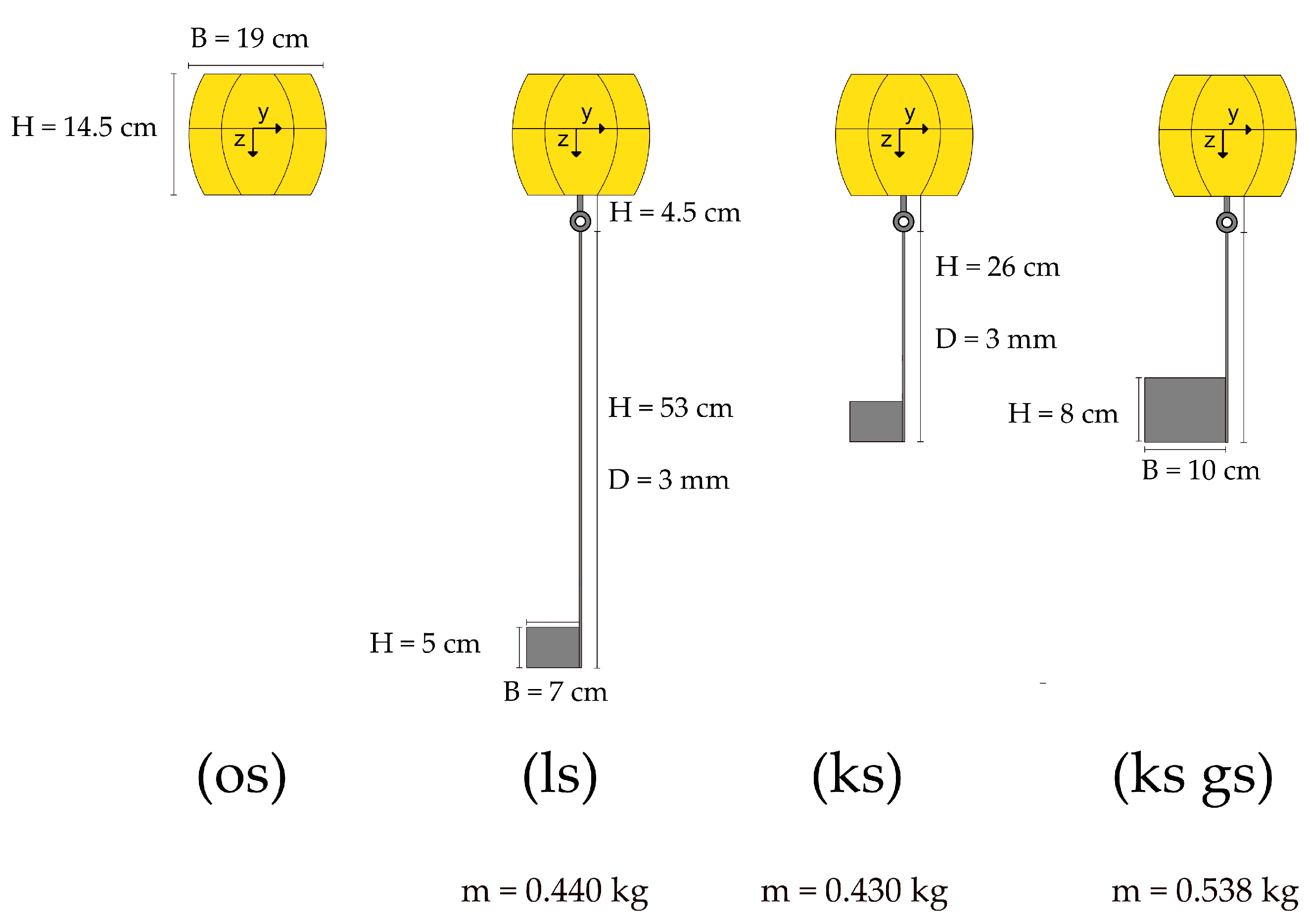To enhance measurement precision, it is crucial to identify the sources of inaccuracies—whether they stem from the Xsens DOT IMU integration or the hydraulic performance of the buoys. We presume that an adapted algorithm for IMU integration combined with the improved hydraulic performance of the buoys can significantly contribute to the precision of the measurement system. To date, the development of specific buoy designs is rarely documented (e.g., in [25,26]), even though there are many publications about the hydraulic performance of wave-buoys [10,11,12,13,14,15,21,22]. Therefore, testing different buoys designs is needed to evaluate the potential for accuracy optimization. We aim to identify the sources of measurement uncertainties arising from both the buoy design and its hydrodynamic behavior, as well as the integration of the inertial measurement unit (IMU), by synthesizing findings from laboratory and field test campaigns. Furthermore, we hypothesize that the accuracy of our measurement system in wave height estimation can be <10 mm by selecting a buoy configuration tested for the best hydraulic performance.

2. Materials and Methods

A combined approach was employed to evaluate the buoys of the wave-monitoring system of recreational boats. Field experiments were conducted to assess the accuracy of the IMU integration, while laboratory experiments examined the hydraulic performance of various buoy configurations. By testing different buoy stabilization systems, the optimal configuration was identified. A flow chart describing the procedure of the study is shown in Figure 1.

To evaluate the accuracy of both the IMU integration and the hydraulic performance of the buoys, three statistical metrics were employed: average absolute deviation (AAD), average relative deviation (ARD), and root mean square error (RMSE). The corresponding equations for these parameters are presented in

Table 1. Parameters used for accuracy evaluation.

Parameter Acronym	Description	Formula
H	wave height	$$H_i=\mathrm{crest}\left(T_i\right)-\mathrm{trough}\left(T_i\right)$$ (1)
T	wave period	$$T_i=t_{zc,2}-t_{zc,1}$$ (2)
$AAD$	average absolute deviation	$$AAD={\displaystyle \frac{1}{N}}\sum _{i=1}^N\left|P_{\mathrm{experiment},\mathrm{i}}-P_{\mathrm{true} \mathrm{reference},\mathrm{i}}\right|$$ (3)
$ARD$	average relative deviation	$$ARD={\displaystyle \frac{1}{N}}\sum _{i=1}^N{\displaystyle \frac{P_{\mathrm{experiment},i}-P_{\mathrm{true} \mathrm{reference},i}}{P_{\mathrm{true} \mathrm{reference},i}}}$$ (4)
$RMSE$	root mean square error	$$RMSE=\sqrt{{\displaystyle \frac{1}{N}}\sum _{i=1}^N{\left(P_{\mathrm{experiment},i}-P_{\mathrm{true} \mathrm{reference},i}\right)}^2}$$ (5)
$\sigma$	standard deviation	$$\sigma =\sqrt{{\displaystyle \frac{1}{N-1}}\sum _{i=1}^N{\left(P_i-\mu \right)}^2}$$ (6)

. Wave height and wave period were determined using the zero-crossing method. Specifically, the wave period was calculated as the interval between two successive upward zero-crossings—i.e., when the signal crosses the zero line from negative to positive. The wave height was defined as the vertical distance between the crest and the trough of the wave within a single period. The conceptual definitions of wave height and period are illustrated in Figure 2, and the associated equations are also provided in Table 1.

2.1. IMU Integration

2.1.1. Algorithm Computing Wave Heights

The processing of wave heights of this wave-monitoring system is based on a modified strapdown algorithm, that was developed at the Working Group of Navigation at the Institute of Geodesy at Graz University of Technology by Härtl [27]. A strapdown algorithm in general integrates the angular rate data once and the acceleration data twice to determine changes in the attitude (or orientation) and position of the object. Thereby, starting values for position, velocity, and attitude are mandatory integration constants.

The main errors of the Xsens DOT IMU namely the biases of accelerometer sensors and angular rate sensors and the scale factors of the accelerometer sensors, were already determined in preliminary research [28]. The recorded inertial raw data were corrected with these calibration parameters before further data processing steps.

Attitude computation: A crucial aspect in the field of inertial navigation is the attitude estimation—the determination of a sensor’s orientation relative to the local-level (l) frame. The primary challenge is to address sensor and integration errors that accumulate throughout this numerical process. For this reason, additional reference observations were used to stabilize the buoy attitude. This was achieved by aligning the magnetometer data with the magnetic north direction and the accelerometer data with the vertical direction, as the gravitational force component remained consistently dominant. The fusion of the orientation computed by integrated angular rate data and the orientation based on the leveling referenced to magnetic and gravity direction was realized with a specifically developed Kalman filter. A detailed documentation, including all necessary formulas, can be found in Härtl’s Thesis [27].

Accelerometer data integration: For a known IMU attitude, the acceleration was integrated twice to receive the height component of the motion of the buoy. For this, the acceleration value ${\mathbf{f}}^{\mathrm{l}}$ rotated into the l-frame was reduced by the gravity acceleration ${\overline{\mathbf{g}}}^{\mathrm{l}}$ obtained from a global gravity model and the Coriolis force ${\mathbf{f}}_{Cor}^{\mathrm{l}}$ due to movement of the object.

$${\dot{\mathbf{v}}}^{\mathrm{l}}\left(t_k\right)={\mathbf{f}}^{\mathrm{l}}\left(t_k\right)+{\overline{\mathbf{g}}}^{\mathrm{l}}-{\mathbf{f}}_{Cor}^{\mathrm{l}}\left(t_k\right)$$

(1)

Integration over time yields the velocity ${\mathbf{v}}^{\mathrm{l}}$.

$${\mathbf{v}}^{\mathrm{l}}\left(t_k\right)={\mathbf{v}}^{\mathrm{l}}\left(t_0\right)+{\int }_{t_0}^{t_k}{\dot{\mathbf{v}}}^{\mathrm{l}}\left(t_k\right)\mathrm{d}t$$

(2)

Here, we enhanced the strapdown algorithm by a trend-correction step. Due to the immanence of errors in the integration of inertial data (and MEMS data in particular), a trend inevitably occurs and our solution accuracy will decrease over time. With the assumption of a periodically oscillating wave body at a tied and anchored position, some restrictions can be made in the integration steps for the velocity and position. Hence, we assumed that the mean of the velocity component over time is always zero. Therefore, we subtracted the linear trend of the last 9 s to compute a detrended velocity from the preliminary velocity resulting from the integration of raw accelerometer data.

The second integration step to obtain the position ${\mathbf{x}}^{\mathrm{l}}$ from the velocity ${\mathbf{v}}^{\mathrm{l}}$

$${\mathbf{x}}^{\mathrm{l}}\left(t_k\right)={\mathbf{x}}^{\mathrm{l}}\left(t_0\right)+{\int }_{t_0}^{t_k}{\mathbf{v}}^{\mathrm{l}}\left(t_k\right)\mathrm{d}t$$

(3)

was done with similar restraints: The mean position of the wave buoy will remain constant over time. Here, a linear trend over the last 8 s was removed from the detrended velocity data. Both detrending parameters of velocity and position were determined empirically with reference data in advance, by processing wave heights from the inertial data with iteratively increasing regression lengths. The trend evaluation was subsequently subjected to a sensitivity analysis to identify the parameter settings that minimized the mean absolute difference between the water surface elevation (WSE) derived from IMU integration and that obtained via MS60 tracking, as described in detail by Härtl [27].

$$\mathrm{mean}\left(\left|\right|{\mathrm{WSE}}_{\mathrm{MS}60}-{\mathrm{WSE}}_{\mathrm{Xsens}}\left|\right|\right)\to min$$

(4)

This optimization yielded ideal regression lengths of $t_v\approx 9$ s and $t_x\approx 8$ s for the trend reduction step. The parameters identified during field experiments were then applied in the evaluation of laboratory tests.

2.1.2. Field Experiments Setup

Field measurements were conducted on 6 June 2024 at Cap Wörth on Lake Wörthersee, Carinthia, Austria (see Figure 3) from 06:40 to 12:32. Since wave exposure varies with bathymetry, the monitoring system covered several water depths from the deep-water zone to the intermediate zone using four buoys (including the master buoy). In addition, four buoys were arranged along the shoreline at a rectangular angle. While a minimum of three buoys is required for accurate wave tracking, the fourth buoy provides redundancy to compensate for potential data gaps or sensor failure. The resulting L-shape of the measurement system was deliberately chosen to enable detection of wave propagation, including speed and direction. To ensure accurate analysis of wave characteristics, the distance between the buoys was set to be at least one typical wavelength (2 to 20 m) depending on the boat type and speed).

A sketch of the measurement concept is shown in Figure 3.

The Xsens DOT was used, which recorded acceleration data, angular rate data, and magnetometer data at a constant rate of 30 Hz. The Leica Nova MS60 MultiStation (MS60) (Heerbrugg, SG, Switzerland) used as reference system has an angular accuracy of target detection (horizontal and vertical) of $1^{″}$ (0.3 mgon) within a distance of 1000 m. The reflector mounted on top of the buoy by a 12 cm long stiff rod atop of the technique box was tracked with automatic target detection and a sampling rate of approx. 20 Hz. Thereby, the reflector reproduced the motion of the buoy and is, therefore, suitable to assess the IMU integration as a true reference.

2.1.3. Data Analysis of the Field Experiments

Time series were synchronized and aligned using the time stamps of GNSS post-processed kinematic (PPK) measurements. The accuracy of IMU integration compared to MS60 measurements was assessed using detected wave heights (determined by the zero-crossing-method, “crest minus trough”). Root mean square error (RMSE) and averaged absolute deviation (AAD) were computed (see Table 1) and classified concerning wave heights (0–50 mm, 50–100 mm, 100–150 mm, >150 mm).

A spectral analysis of both data series was performed in Matlab® version R2023b. Wavelet analysis enables a time-frequency representation of the given dataset, showing all occurring wave amplitudes at a specific scale resp. frequency at a specific time. The term scale in wavelet theory represents the term period in Fourier analysis. A wavelet coherence of Xsens DOT IMU data and MS60 data was computed to compare the results in the time and frequency domains. Wavelet coherence measures the cross-correlation of two wavelet transform functions based on time and frequency, expressed as a quantity between 0 and 1 [29].

2.2. Buoy Design

2.2.1. Laboratory Experiments Setup

Laboratory experiments were examined to assess the hydraulic performance of various buoy configurations in the hydraulic laboratory of the Institute of Hydraulic Engineering and Water Resources Management, Graz University of Technology, Graz, Austria on 26 April, 17 May, 15 July, and 3 September 2024. The experiments were conducted at the prototype scale. To evaluate how accurately the buoys represent real wave patterns, harmonic waves were measured for five minutes in a wave flume using a potentiometric level sensor, while simultaneously the buoy floated attached with a Xsens DOT. The used potentiometric sensor was a CONDURIX (FAFNIR®, Hamburg, Germany), with a sampling rate of 60 Hz and a measurement linearity of $\pm 1$ mm (or $\pm 2$ %) and replicability of $0.5$ mm. It was equipped with an additional rod to generate a counter-potential. The experimental setup, including relevant dimensions, is shown in Figure 4. The buoy’s position within the wave flume was not fixed directly to the reference sensor but remained partly free-floating to represent the actual field application. To ensure a correspondence between the wave buoy and reference sensor, the buoy was mounted along a rope at a fixed position along the flume. Two suitable positions were identified (p1 and p2 in Figure 4) that had been thoroughly tested in preliminary experiments to ensure the buoy floats at the same level as the reference sensor. For the high-frequency wave configurations s16n100 and s22n900 the buoy was mounted at p2, whereas to low-frequency configurations it was mounted at p1. To prevent reflections at the end of the flume, a plate was implemented with an inclination of 1:3. A constant discharge of 25 L/s guaranteed a balanced water volume within the flume. The mean water level ranged between $0.6$ and $0.65$ m.

Based on preliminary tests, a wave generator was developed that replicated the range of relevant boat waves characterized by wave heights ranging from 0.04–0.28 m and periods from 1–3 s [3,7,9] The wave generator consists of a paddle, hinged at a fixed position, rotating with a defined speed and stroke extend. Due to the geometric limitations of the flume, wave heights of up to approximately $0.15$ m were possible. The period varied between $0.9$ and $1.8$ s. The tested configurations are summarized in

Table 2. Tested wave configurations in the flume.

Max. Stroke Extent [m]	Motor Velocity [1/min]	Position	Alias
$0.22$	500	p1	s22n500
$0.16$	700	p1	s16n700
$0.16$	1000	p2	s16n1000
$0.22$	900	p2	s22n900

presenting the parameters of wave generator and positions of the buoys, including the aliases, used in the following for the identification of the wave configuration.

Table 3. Tested wave configurations in the flume including their mean values $\mu$ and standard deviations $\sigma$ concerning wave heights and periods for the test runs of the support buoy ks.

Parameter	Acronym	s22n500	s16n700	s16n1000	s22n900
Wave height [mm]	$\sigma$	1.64	1.92	4.46	9.12
	$\mu$	38.3	83.78	127.34	153.84
Period [s]	$\sigma$	0.02	0.01	0.01	0.01
	$\mu$	1.78	1.26	0.88	0.98
H class. [mm]		0–50	50–100	100–150	>150
T class. [s]		$1.8$	$1.3$	$0.9$	$1.0$

describes the wave period and the wave height of the four tested wave configurations during 5 min measurements concerning the mean value and standard deviation. Since the standard deviation remains small and amounts to 2–6% of the mean value, we assume that test runs act quasi-stationary. The wave classifications concerning H and T are included in this table for comparability with the field test.

The buoyancy of the plastic floating body of the support buoys amounted to 1.8 kg and 8.5 kg for the master buoy. The stabilization rod was made of aluminum, whereas the lower stabilizers were made of steel sheet. Different geometries of buoy stabilizers and stabilization length were tested to optimize the measurement accuracy of the support buoy and are introduced in Figure 5. The findings for the best hydraulic behavior of the support buoys were used for designing the master buoy. The rod length and the size of the lower stabilizers were arranged in proportion to the buoy height. Additionally, for the master buoy, a second stabilizer was tested below the buoy made of Plexiglas, weights down at the stabilization rod by cuboids, and a weighted plate below the buoy. The dimensions of each configuration are shown in Figure 6. Each buoy type was tested with four different wave configurations (see Table 2) to account for a wide range of wave impacts.

2.2.2. Data Analysis of the Laboratory Experiments

The comparison between the wave data by the potentiometric sensor and by the IMU was the basis for identifying the hydraulic performance of the tested buoys and concluding the most accurate buoy configuration. Both datasets were clipped to the identical time series, excluding the first approx. 10 s that were used for estimating the parameters of the IMU integration. Considering this subtraction in time, a time frame between 4 min 50 s and 5 min was available for further evaluation. However, despite these measures, it is still possible that the wave buoy and the potentiometric sensor may not measure the same wave at the same time stamp, because the global time stamp of the IMU (date and time) is precise within 1 s, whereas the internal time stamp (recording frequency) is 1/30th second. We decided to work with wave packages to address these inaccuracies in wave identification. This approach enables a more statistical approach without compromising the quality of the results. We tested different wave packages containing varying numbers of waves, as illustrated for the wave configuration s16n700 in Figure 7. For this sensitivity analysis, we used the data recorded by the potentiometric sensor. Our analysis revealed that wave height exhibited slight variations over time (see also the standard deviations in Table 3), due to water losses and the gradual refilling of the wave tank. It was noted that wave packages containing more than 10 waves resulted in an misjudgment of the individual wave height in all wave configurations. To address this, we decided to use wave packages of 5, which would accurately represent time-dependent wave heights while compensating for deviations in time stamps. The wave height and period were evaluated using the zero-crossing method, applying the mean water level as zero-line. The data analysis was conducted using Matlab® version R2023b.

To identify trends in the hydraulic behavior, all AAD and ARD (both concerning wave height and period) and RMSE values comparing each wave package of the IMU sensor with the potentiometric sensor were calculated and averaged for each tested wave configuration. Their mean values (averaged for the four wave configurations) and the range of minimum and maximum AAD were determined. The mean standard deviation (average of the four wave configurations) for the buoy configurations of the master buoy was calculated.

3. Results

Before combining and interpreting the sources of inaccuracy, the results of the field and the laboratory experiments are evaluated separately.

3.1. IMU Integration

The IMU integration matched the true reference of the MS60 very precisely. The assessment of the IMU integration showed an overall AAD of $1.9$ mm and RMSE of $3.1$ mm. Figure 8 visualizes the timeline of an exemplary wave package characterized by a maximum wave height of about $90$ mm by comparing the Xsens DOT data and the MS60 data.

With increasing wave height, the consistency between the Xsens DOT and MS60 decreased. For wave heights < 50 mm, the AAD was $1.6$ mm, whereas for wave heights > 150 mm, the AAD rose to $9.1$ mm. Since the number of detected waves < 100 mm contributed to most of the total detected waves, the overall AAD and RMSE yielded a low extent of $1.9$ mm and $3.1$ mm, respectively.

Table 4. IMU integration results evaluated by wave height.

H Classification [mm]	Quantity	RMSE [mm]	AAD [mm]
<50	9837	$2.4$	$1.6$
50–100	1158	$5.2$	$3.5$
100–150	161	$8.1$	$6.2$
≥150	71	$11.4$	$9.1$
all	$11,227$	$3.1$	$1.9$

shows the error composition for all analyzed wave classes.

Concerning the period of wave components, the Xsens DOT and MS60 data coincided very well in the ranges between $0.5$ and 4 s (compare Figure 9c). The PSD of both the Xsens DOT and MS60 data reveals a strong signal within the period range of 1 to 4 s, corresponding to the characteristic wave patterns generated by recreational boating activity. Signal strength decreases noticeably in the 4 to 8 s range, and no distinct signal is observed for periods exceeding 8 s. These frequency-dependent patterns are consistently reflected in the coherence analysis. In the range of strong wave signal—between 1 and 4 s—the computed wavelet coherence reached between $0.8$ and 1. The overall coherence decreased for periods larger than 4 s, as it did with periods smaller than $0.5$ s. If the wave signal is pronounced in wave components of longer periods, the two datasets agree in the wave spectrum up to 8 s. Those large wave periods typically occur at the beginning of the diverging waves, which cause a crisp signal that increases in frequency with time. This can be seen, e.g., in the time frame between 2:30 and 3:00 min within the plots in Figure 9. The long-period wave components provided less pronounced wave signals than wave components in frequency ranges between 4 and 1 s.

3.2. Buoy Design

Both support and master buoys were tested under four different wave exposures (Table 2). The results were evaluated concerning AAD, absolute deviation range, and averaged relative deviation (ARD). The evaluation of the IMUs was computed without considering magnetic orientation since lateral orientation could be neglected in the flume. The raw data from the laboratory test results are presented as boxplots in Figure A1 for the tested support buoys and Figure A2 for the master buoys.

3.2.1. Support Buoy

All tested support buoy types accurately reproduced the wave periods within $0.01$ s. However, the wave height measurements showed a higher deviation. The buoy without a stabilization system both under- and overestimated the actual wave heights, depending on the wave configuration. This led to the largest total AAD and widest absolute deviation range (Figure 10I). The long ls and short stabilizers ks exhibited similar mean AAD and absolute deviation ranges (Figure 10I), showing comparable patterns in their AAD and ARD for different wave configurations (Figure 11I). In contrast, the larger stabilizers ks gs produced greater AAD and tended to underestimate wave heights in terms of ARD significantly compared to ks and ls (Figure 11II). The configuration s22n500, which represents the smallest wave heights with the longest periods among the tested wave configurations, produced the lowest ARD, except for the buoy without a stabilization system os. Conversely, the wave configurations s16n700 and s22n900, representing wave classifications between 100 and >150 mm and periods between 1 and $1.3$ s, generated the largest relative deviation across all support buoy types. The wave configuration s16n1000, representing a high wave classification (100–150 mm) with a small period ($0.9$ s), resulted in slightly smaller AAD and ARD compared to the configurations s16n700 and s22n900.

The same trends can be seen in the results for the RMSE, presented in

Table 5. RMSE in [mm] of the tested support buoys.

Wave Configuration	os	ls	ks	ks gs
s22n500	8.18	0.35	1.22	3.50
s16n700	11.36	12.36	14.46	21.58
s16n1000	10.47	8.27	7.09	17.75
s22n900	40.80	22.00	23.52	21.31
all	24.42	14.82	16.07	19.67

. The buoy without stabilization system os shows the highest overall RMSE, whereas support buoys ks and ls show similar smaller ranges between 14 and 16 mm.

3.2.2. Master Buoy

The design of the master buoy has been scaled to align with the dimensions of the support buoy ls, incorporating a short stabilization rod and small stabilizers. This configuration, together with configuration ls, demonstrated the best performance during the laboratory tests. Additionally, the ks buoy enables the same testing configuration without the need to raise the water level, ensuring that the master buoy remains freely floating. This would not be possible by scaling the ls-configuration.

Like the support buoys, the tested master buoy designs demonstrated excellent accuracy in reproducing the wave period. For buoy type G, the measured period deviated by $0.1$ s, while all other designs had deviations within $0.01$ s.

Among the tested buoy types, buoy type J exhibited the smallest AAD of less than 10 mm, whereas type G showed the highest (Figure 12I). Unlike the support buoys, the master buoy types did not consistently underestimate the actual wave heights. The ARD evaluation (Figure 12II) presents a more nuanced picture.

The results indicate that buoy types G, I, which incorporated a secondary mass element at the base, tend to underestimate wave heights, particularly under the s22n900 configuration (Figure 12II). Notably, this effect was absent in type K, which also incorporated a secondary mass element. This aligns with observations from other buoy types equipped with a weighted plate beneath the buoy (H, J and K), which tended to overestimate wave heights in case of configuration s22n900.

While buoy type A demonstrated a greater AAD and ARD compared to buoy type B under the s22n900 wave configuration, the presence of an additional stabilizer beneath the buoy A generally reduced its AAD and ARD. For all other wave configurations except s22n900, buoy A consistently exhibited a smaller deviation than buoy B. A similar trend was observed when comparing buoy types J with H. In line with the results of the AAD evaluation, the RMSE showed similar trends as shown in

Table 6. RMSE in [mm] of the tested master buoys.

Wave Configuration	A	B	G	H	I	J	K
s22n500	1.87	2.41	8.79	2.31	6.00	1.09	4.95
s16n700	11.60	15.18	10.08	10.19	9.01	2.82	6.32
s16n1000	7.05	20.73	16.44	12.72	12.80	15.37	12.57
s22n900	33.11	21.25	36.39	25.10	33.20	16.21	22.39
all	19.13	17.99	22.55	16.13	19.96	12.46	14.50

. Buoy type J presented the smallest RMSE with 12.46, followed by buoy type K with 14.50 mm. The highest RMSE was calculated for the buoy type G, which also showed the greatest mean AAD and maximum AAD in Figure 10II.

Analysis of the averaged absolute deviation and deviation range revealed that buoys equipped with an additional stabilizer beneath the buoy exhibit improved performance in both AAD and ARD. Furthermore, buoys featuring a weighted plate below the buoy (types H, J, and K) consistently achieved the lowest AAD (Figure 10II). Combining a weighted plate with a stabilizer, as observed in types J and K, results in the smallest absolute deviation ranges (Figure 10II).

In addition to the minimal, maximal, and mean AAD, we also computed the AAD range and the mean standard deviation of the wave heights $\sigma (H_{IMU}$) measured by the Xsens DOT sensor.

Table 7. Assessment of the stabilization system of the tested master buoys. Cells highlighted in green indicate superior hydrodynamic performance, where the computed value for a specific buoy type is lower than the overall mean.

Configuration	A	B	G	H	I	J	K	Mean Value
Plate				x		x	x
Second stabilizer	x				x	x	x
Second weight			x		x		x
Min AAD	1.47	2.16	7.76	2.13	5.82	0.86	4.86	3.58
Max AAD	29.51	18.61	35.71	24.37	31.98	13.28	20.65	24.87
AAD Range	28.03	16.45	27.95	22.24	26.16	12.42	15.78	21.29
Mean AAD	12.00	13.41	16.27	11.40	14.21	6.94	10.55	12.11
Mean $\sigma \left(H_{IMU}\right)$	4.63	5.06	6.38	3.74	4.46	3.69	4.27	4.60

summarizes these results for each buoy configuration, indicating the stabilization system employed. If the computed value for a specific buoy type is lower than the overall mean, it is highlighted in green, denoting superior hydrodynamic performance. Among all configurations, buoy type J demonstrated the best overall performance across all evaluated parameters, consistent with prior findings. Buoy types equipped with a plate beneath the float (H, J, K) performed better than the mean in at least four out of five parameters, suggesting a beneficial influence of this stabilization method. In contrast, buoy types incorporating a secondary weight at the bottom (G, J) tend to exhibit poorer performance, with only zero or one parameter outperforming the mean. While buoy type B, which lacks any additional stabilization, appears to outperform type A based on the mean values reported in Table 7, the ARD analysis shown in Figure 12II suggests that the secondary stabilizer effectively compensates for the underestimation observed in type A. This effect may explain why type J outperforms type K.

4. Discussion

Both field and laboratory tests yielded critical datasets for assessing the measurement accuracy of the novel wave buoy system specifically designed for monitoring recreational boat-induced waves. Testing various buoy types emphasized the importance of the buoy designs for optimizing hydraulic behavior and thereby the measurement accuracy of the wave-monitoring system.

4.1. Measurement Accuracy of IMU Integration

The data analysis of IMU integration confirmed a very high accuracy in the overall AAD of less than 2 mm concerning wave heights. The calculated deviations are based on the assumption that the MS60 acted as a true reference. Since the position of the reflector and the Xsens DOT differ slightly, those deviations could also partly originate from the tilted positions of the buoys during the wave transition. Observed waves are characterized by long wavelengths, small amplitude, and small wave steepness, whereby we expect this error source to be negligible.

In the case of the most frequent waves of wave heights < 50 mm, the AAD amounted $1.6$ mm. Even though some buoy types could follow this AAD (ks, ls, A, J), most of the buoys overtopped the accuracy range of the IMU. For wave heights greater than 50 mm, the AAD of the Xsens DOT increased to $9.1$ mm. In case of wave heights of 100–150 mm, the AAD amounted to $6.2$ mm. In contrast, lab tests generated mainly higher AAD of the 5–41 mm for this wave class. This means that the overall accuracy in wave measurements by Xsens DOT-equipped buoys was limited by the hydraulic performance of these wave-buoys rather than IMU integration. Comparing these results with those of the previous study by Mascher and Berglez [23], the accuracy improved significantly, with the maximum RMSE decreased from 43 mm to $11.5$ mm. In the previous study, accuracy was assessed using the averaged RMSE over the entire data recording, which may overestimate the RMSE of wave height, as minor temporal shifts can cause substantial deviations in wave measurements. Furthermore, Mascher and Berglez [23] reported that wind intensity affects the accuracy of the measurement. The wind effect could not be quantified in the previous study by Mascher and Berglez [23] but was instead described qualitatively as either “very windy” or “less windy”. Under windy conditions, wave generation is intensified, potentially leading to increased wave heights and, as shown in the present study, greater deviations in measurement accuracy. A comprehensive quantitative assessment of wind influence would require the integration of an anemometer on the buoy, as wind speed and direction are highly site-specific. Moreover, the measurement approach utilizing the MS60 in combination with a reflector mounted on the buoy may be unsuitable in windy conditions. The reflector, positioned atop a rod approximately 12 cm in length, is susceptible to positional skewing due to wind-induced tilting of the buoy. This may increase the vertical displacement between the IMU and the reflector, potentially leading to greater discrepancies between IMU-derived wave heights and MS60 reference measurements. The reduced accuracy in IMU integration observed in the previous study may thus be more attributable to limitations in the measurement setup under windy conditions than to actual errors in wave height estimation. Due to the lack of site-specific, quantitative wind data, this effect could not be evaluated further in the present study. However, integrating an anemometer in the measurement system would enable the collection of wind data, facilitating the analysis of wind effects on measurement accuracy and offering valuable insights for distinguishing between wind-generated and vessel-induced waves. In future research, artificial intelligence could be employed to enhance and automate both the detrending algorithm for the IMU integration and the filtering process, enabling the extraction of relevant information regarding wave contributions, whether wind- or vessel-induced.

Periods > 4 s and <0.5 s might be underestimated using the Xsens DOT. Since the power of those waves was less pronounced in the recorded dataset of the field test, the identification of those waves might be limited. The boat-induced waves of our interest range in periods between 1 and 3 s [3,9], which matches the range of strong wavelet coherence. Short wind waves (ripples) might not be represented correctly in the Xsens DOT wave spectrum, like internal waves characterized by very long periods. However, the measurement units allow a high-resolution detection of wind waves, comparable to other MEMS-based buoys [15].

4.2. Measurement Accuracy of Wave Buoys

The measurement accuracy of wave periods was found to be at least $0.05$ s, while wave heights were reproduced with an overall AAD of less than 20 mm. This is in a comparable range with other well-performing wave-buoys [18,19], proving the reliability and operability of our wave-monitoring system. However, the maximum error reached over 4 cm for the support buoy without stabilization (os), which exhibited the poorest performance across all error evaluations. The tested stabilizers significantly enhanced measurement accuracy. Surprisingly, the length of the stabilization rod appeared to have minimal influence on measurement accuracy. Both absolute and relative deviation evaluations of the buoy types ks and ls yielded nearly identical results.

In contrast, increasing the size of the stabilizers, as in the ks gs configuration, increased the AAD while maintaining a consistent AAD range. However, the relative deviation for ks gs demonstrated a stronger tendency to underestimate wave heights. This underestimation may be attributed to the increased mass associated with the larger stabilizers. Under the hydraulic exposure conditions tested in this study, the larger stabilizers may have been too heavy to respond with sufficient sensitivity, as indicated by the underestimation of results compared to the reference measurements. However, under conditions of stronger wave exposure, these larger stabilizers may prove to be more suitable due to their greater mass and potential for improved stability in high-energy environments.

Laboratory tests conducted in a wave flume demonstrated that a master buoy configured as J could achieve a mean absolute measurement accuracy of less than 1 cm. This configuration combines two types of stabilizers with added weights at the bottom of the stabilization rod and beneath the buoy. These weights lower the center of mass, thereby enhancing stability. Interestingly, doubling the weight at the bottom of the buoy negatively impacted measurement accuracy, whereas the weighted plate below the buoy helped balance relative deviations. The second weight down at the stabilization rod tends to enhance inertness, similar to the effect of the greater stabilizers in the case of the support buoys, and make the measurement unit less sensitive.

The stabilizer below the buoy effectively reduced the underestimation of wave heights; however, this effect was not observed for buoy types A and B under the s22n900 configuration. Instead, a counteracting effect was noted, which could potentially be attributed to defective measurements or IMU evaluations. The stabilizer’s effect aligned with the overall trends for all other wave configurations.

For buoy types G and I, the double mass at the bottom of the stabilization rod significantly underestimated wave heights. This may be due to the excessively low center of mass acting too strongly against surface elevation accelerations. Conversely, the weighted plate beneath the buoy tended to increase the measured wave heights, likely due to its effect of raising the center of mass. Those buoy types equipped with a plate beneath the float demonstrated good hydraulic performance, indicating that this stabilization method has a positive effect on measurement accuracy.

A comparison of the optimal buoy configurations for both support and master buoys reveals that the support buoys generally yield lower measurement accuracy. This reduction in performance is likely attributable to their decreased weight, which renders them more susceptible to tilting and, consequently, more prone to measurement errors. The heaviest buoy configuration did not exhibit the best hydrodynamic performance. Instead, the experimental results highlight the critical importance of weight distribution. Specifically, positioning the weight closer to the float appears to enhance the buoy’s hydrodynamic behavior, whereas placing the weight at the bottom tends to diminish performance. These findings suggest the necessity of carefully balancing stability and responsiveness. Although increasing weight may improve stability, it does not guarantee improved performance. Therefore, future investigations could explore the effects of incorporating additional weights beneath the float in support buoy designs to further optimize measurement accuracy without compromising sensitivity.

4.3. Implications on Wave Monitoring System and Its Applicability

The algorithm for integrating the IMU data is tailored to detecting wave heights typically induced by recreational boats. This means that other wave phenomena like tides or short wind waves with periods $<0.5$ s cannot currently be evaluated accurately. Since short wind waves imply low wave energy compared to boat waves, the total wave evaluation is only slightly affected by neglecting short wind waves. A mean AAD of less than 10 mm in case of the best wave configuration among the tested wave configuration allows a detailed evaluation of wave impacts on lakes, even in case of small wave heights. Even though waves characterized by wave heights $<0.05$ m might not be relevant for erosive processes directly impacting macrophytes, they can significantly contribute to the total wave energy occurring on a lake, since they appear more frequently compared to greater wave heights (see Table 4). Furthermore, small-amplitude waves are important in the case of wave-filtering, to identify the relative contributions of wind and vessel-induced waves. To date, the system is not applicable in great lakes or marine environments, where the general wave pattern is characterized by wave periods $>4$ s. Even though we could see that wave components characterized by periods up to 8 s can be detected accurately with our system, it is not validated for environments characterized by peak periods > 4 s. The same applies in the case of greater vessels like passenger or container ships that can cause waves with peak periods larger 4 s [30,31,32]. Since the data acquired in both the laboratory experiments and field experiments do not imply long-period waves, the results and applicability of this study are limited to the frequency band of recreational vessel-induced waves. We expect that the tested wave-buoys are not suitable for waves characterized by wave heights $>0.5$ m, because the length of the stabilization system would range within the wave crest and could not act as a stabilizer. This means that for maritime environments or great lakes, where wind-induced wave generation results in waves greater than 0.5 m, the monitoring system is not applicable. The same applies to lakes that are used by great ships, inducing waves with greater wave heights than those tested in this study. Instead, due to the small dimensions of the buoys, the system is recommended for shallow waters, which allows small-scaled wave exposure recording that can be especially relevant for ecological and morphodynamic assessments. Due the floating buoy system, no anchorage interrupts the flow field on the ground that might cause unfavorable scouring effects. The measurement system is suitable for typical inland lakes with limited fetch lengths that are used for recreational boating. Since the impact of vessel-induced waves on total wave energy reduces with fetch length [3], wave monitoring of recreational boats is particularly relevant.

5. Conclusions

Boat-induced waves can initiate ecological processes that may change lake ecosystems. To control and limit those effects, a precise wave-monitoring system is crucial. The tested wave buoys are suitable for monitoring waves characterized by wave components with periods between $0.5$ and 8 s. The tested buoys achieved a measurement accuracy concerning wave heights in terms of mean AAD of less than 20 mm and for best buoy configuration less than 10 mm for the tested wave configuration. The design and buoy type can significantly affect measurement accuracy, especially in the high-frequency band of wave classifications we tested in the wave flume. The results highlight the significance of buoy design in overall measurement accuracy, particularly for waves exceeding wave heights of >5 mm. The tested buoy designs offer viable design options that can contribute to the accuracy enhancement of existing wave buoys. The measurement system is particularly suitable for typical inland lakes with limited fetch lengths that are used for recreational boating. The applicability of the system for wave motions characterized by peak period > 4 s requires further investigation. Since wavelength and wave propagation speed decrease in shallower water, it is reasonable to implement a monitoring system covering relevant zones of water depth related to the photic zone (macrophyte growth) and bathymetry (sediment processes).

References

1. Millennium Ecosystem Assessment. Ecosystems and Human Well-Being; Island Press: Washington, DC, USA, 2005; Volume 5. [Google Scholar]
2. Valbuena, S.; Schladow, S.; Bombardelli, F. Boat Effects on Lake Water Clarity and the Efficacy of a No-Wake Zone Policy. Lake Reserv. Manag. 2024, 41, 16–33. [Google Scholar] [CrossRef]
3. Houser, C.; Carswell, A.; Chittle, B.; Johnson, G.; Caschera, A.; Smith, A. Relative Energy and Perceived Impact of Vessel-Generated Waves in Fetch-Limited Environments. Lake Reserv. Manag. 2024, 40, 285–302. [Google Scholar] [CrossRef]
4. Liddle, M.J.; Scorgie, H.R.A. The Effects of Recreation on Freshwater Plants and Animals: A Review. Biol. Conserv. 1980, 17, 183–206. [Google Scholar] [CrossRef]
5. Gabel, F.; Lorenz, S.; Stoll, S. Effects of Ship-Induced Waves on Aquatic Ecosystems. Sci. Total Environ. 2017, 601–602, 926–939. [Google Scholar] [CrossRef]
6. Sorensen, R.M. Prediction of Vessel-Generated Waves with Reference to Vessels Common to the Upper Mississippi River System; Technical Report 4; U.S. Army Engineer District: Washington, DC, USA, 1997; Available online: https://api.semanticscholar.org/CorpusID:132716271 (accessed on 2 November 2023).
7. Maynord, S. Wave Height from Planing and Semi-Planing Small Boats. River Res. Appl. 2005, 21, 1–17. [Google Scholar] [CrossRef]
8. Liedermann, M.; Tritthart, M.; Gmeiner, P.; Hinterleitner, M.; Schludermann, E.; Keckeis, H.; Habersack, H. Typification of Vessel-Induced Waves and Their Interaction with Different Bank Types, Including Management Implications for River Restoration Projects. Hydrobiologia 2024, 729, 17–31. [Google Scholar] [CrossRef]
9. Sheng, S.J.; Ouahsine, A.; Smaoui, H.; Sergent, P. Numerical Prediction of Ship-Generated Waves in Restricted Channel. In Proceedings of the Marine 2011 Computational Methods in Marine Engineering IV, Lisbon, Portugal, 28–30 September 2011; pp. 146–156. [Google Scholar]
10. Knight, P.; Bird, C.; Sinclair, A.; Higham, J.; Plater, A. Beach Deployment of a Low-Cost GNSS Buoy for Determining Sea-Level and Wave Characteristics. Geosciences 2021, 11, 494. [Google Scholar] [CrossRef]
11. Guercio, A.; Kumar, D.; Cirrincione, M.; Raimondi, F.; Montalbano, A.; Frazitta, V. Improvement of a Low-Cost Buoy for the Measurement of the Sea Wave Weather. In Proceedings of the OCEANS 2021: San Diego–Porto, San Diego, CA, USA, 20–23 September 2021. [Google Scholar] [CrossRef]
12. Schanzle, J.A.; Wood, J.D.; Terray, E.A. The use of low-cost inertial sensors to improve deep water wave and current measurements from subsurface moorings. In Proceedings of the 2014 Oceans—St. John’s, St. John’s, NL, Canada, 14–19 September 2014; pp. 1–6. [Google Scholar] [CrossRef]
13. Liu, Y.; Li, M.; Liu, Y.; Wang, Y.; Jiang, S.; Wang, Y.; Tian, L.; Qiao, F. Real-Time Precise Measurements of Ocean Surface Waves Using GNSS Variometric Approach. Int. J. Appl. Earth Obs. Geoinf. 2022, 115, 103125. [Google Scholar] [CrossRef]
14. Zhong, Y.Z.; Chien, H.; Chang, H.M.; Cheng, H.Y. Ocean Wind Observation Based on the Mean Square Slope Using a Self-Developed Miniature Wave Buoy. Sensors 2022, 22, 7210. [Google Scholar] [CrossRef]
15. Yurovsky, Y.; Dulov, V. MEMS-based Wave Buoy: Towards Short Wind-Wave Sensing. Ocean Eng. 2020, 217, 108043. [Google Scholar] [CrossRef]
16. Raghukumar, K.; Chang, G.; Spada, F.; Jones, C.; Janssen, T.; Gans, A. Performance Characteristics of “Spotter”, a Newly Developed Real-Time Wave Measurement Buoy. J. Atmos. Ocean. Technol. 2019, 36, 1127–1141. [Google Scholar] [CrossRef]
17. Lancaster, O.; Cossu, R.; Boulay, S.; Hunter, S.; Baldock, T. Comparative Wave Measurements at a Wave Energy Site with a Recently Developed Low-Cost Wave Buoy (Spotter), Adcp, and Pressure Loggers. J. Atmos. Ocean. Technol. 2021, 38, 1019–1033. [Google Scholar] [CrossRef]
18. Knight, P.; Bird, C.; Sinclair, A.; Plater, A. A Low-Cost GNSS Buoy Platform for Measuring Coastal Sea Levels. Ocean. Eng. 2020, 203, 107198. [Google Scholar] [CrossRef]
19. Apel, H.; Hung, N.G.; Thoss, H.; Schöne, T. GPS Buoys for Stage Monitoring of Large Rivers. J. Hydrol. 2021, 412–413, 182–192. [Google Scholar] [CrossRef]
20. Beckman, J.; Long, J. Quantifying Errors in Wind and Wave Measurements from a Compact, Low-Cost Wave Buoy. Front. Mar. Sci. 2022, 9, 966855. [Google Scholar] [CrossRef]
21. Yurovsky, Y.; Dulov, V. Compact Low-cost Arduino-Based Buoy for Sea Surface Wave Measurements. In Proceedings of the 2017 Progress in Electromagnetics Research Symposium-Fall (PIERS-FALL), Singapore, 19–22 November 2017; pp. 2315–2322. [Google Scholar] [CrossRef]
22. Ladd, C.; Vovides, A.; Wimmler, M.C.; Schwarz, C.; Balke, T. Monitoring Tides, Currents, and Waves along Coastal Habitats Using the Mini Buoy. Limnol. Oceanogr. Methods 2014, 22, 619–633. [Google Scholar] [CrossRef]
23. Mascher, K.; Berglez, P. Wave Height Determination Based on Low-Cost Inertial Measurements Unit: Potential and Challenges for an Innovative Environmental Monitoring System. Österreichische Z. Vermess. Geoinf. 2024, 2024, 54–62. [Google Scholar]
24. Zhou, B.; Watson, C.; Legresy, B.; King, M.A.; Beardsley, J.; Deane, A. GNSS/INS-Equipped Buoys for Altimetry Validation: Lessons Learnt and New Directions from the Bass Strait Validation Facility. Remote Sens. 2020, 12, 3001. [Google Scholar] [CrossRef]
25. Nagai, S.; Oda, K.; Kurata, K. Studies of the Navigation Buoy for Strong Tidal Currents and Large Waves. Coast. Eng. Proc. 1972, 1972, 93. [Google Scholar] [CrossRef]
26. International Association of Marine Aids to Navigation and Lighthouse Authorities (IALA). G1099—The Hydrostatic Design of Buoys; Technical report; IALA: Saint-Germain-en-Laye, France, 2022. [Google Scholar]
27. Härtl, R. Wellenhöhenbestimmung mittels Low-Cost-Inertialsensorik. Master’s Thesis, Graz University of Technology, Institute of Geodesy, Working Group Navigation, Graz, Austria, 2025. [Google Scholar]
28. Moder, T.; Reitbauer, C.; Dorn, M.; Wieser, M. Calibration of Smartphone Sensor Data Usable for Pedestrian Dead Reckoning. In Proceedings of the 2017 International Conference on Indoor Positioning and Indoor Navigation (IPIN), Sapporo, Japan, 18–21 September 2017; pp. 1–8. [Google Scholar] [CrossRef]
29. Torrence, C.; Compo, G.P. A Practical Guide to Wavelet Analysis. Bull. Am. Meteorol. Soc. 1998, 79, 61–78. [Google Scholar] [CrossRef]
30. Hofmann, H.; Lorke, A.; Peeters, F. The Relative Importance of Wind and Ship Waves in the Littoral Zone of a Large Lake. Limnol. Oceanogr. 2008, 53, 368–380. [Google Scholar] [CrossRef]
31. Curtiss, G.M.; Osborne, P.D.; Horner-Devine, A.R. Seasonal Patterns of Coarse Sediment Transport on a Mixed Sand and Gravel Beach Due to Vessel Wakes, Wind Waves, and Tidal Currents. Mar. Geol. 2009, 259, 73–85. [Google Scholar] [CrossRef]
32. Houser, C. Relative Importance of Vessel-Generated and Wind Waves to Salt Marsh Erosion in a Restricted Fetch Environment. J. Coast. Res. 2010, 26, 230–240. [Google Scholar] [CrossRef]
Figure 1. Flow chart of the procedure of the study.
Water 17 01345 g001
Figure 2. Definitions of used wave-parameters: H—wave height, T—wave period.
Water 17 01345 g002
Figure 3. Measurement concept of buoy system including master and support buoys exposed to characteristic waves induced by a boat. The map shows the field study site, Cap Wörth at Lake Wörthersee, Carinthia.
Water 17 01345 g003
Figure 4. Wave flume used for laboratory test and its experimental test-setup.
Water 17 01345 g004
Figure 5. Tested buoy designs of the support buoy os—without any stabilization, ls—long stabilization, ks—short stabilization, ks gs—short stabilization and large stabilizators.
Water 17 01345 g005
Figure 6. Tested buoy designs of the master buoy ABGHIJK.
Water 17 01345 g006
Figure 7. Sensitivity analysis for a suitable wave package selection with n number of individual waves, using the example of wave configuration s16n700.
Water 17 01345 g007
Figure 8. Water surface elevation (WSE) of integrated Xsens DOT data and MS60 reference data including detected crests and troughs.
Water 17 01345 g008
Figure 9. Comparison of computed PSD (power spectral density plot) with clearly visible boat wave components.
Water 17 01345 g009
Figure 10. Total AAD including the individual minimum and maximum absolute deviations (absolute deviation range) for support buoys (I) and master buoys (II).
Water 17 01345 g010
Figure 11. Error evaluation for the support buoy. Matrix plot of AAD (I) and ARD (II) (wave height) for all tested designs against all tested wave configurations.
Water 17 01345 g011
Figure 12. Error evaluation for the master buoy. Matrix plot of AAD (I) and ARD (II) (wave height) for all tested designs against all tested wave configurations.
Water 17 01345 g012