


Understanding Climate Change Impacts on Streamflow by Using Machine Learning: Case Study of Godavari Basin


 , , ,
, , ,  and
and
Abstract
1. Introduction
1.1. Research Gap of the Study Area
1.2. Objectives of the Research Work
2. Materials and Methods
2.1. Location
2.2. Data Collection and Sources
2.2.1. CMIP6 Model Data
2.2.2. Conceptual Models
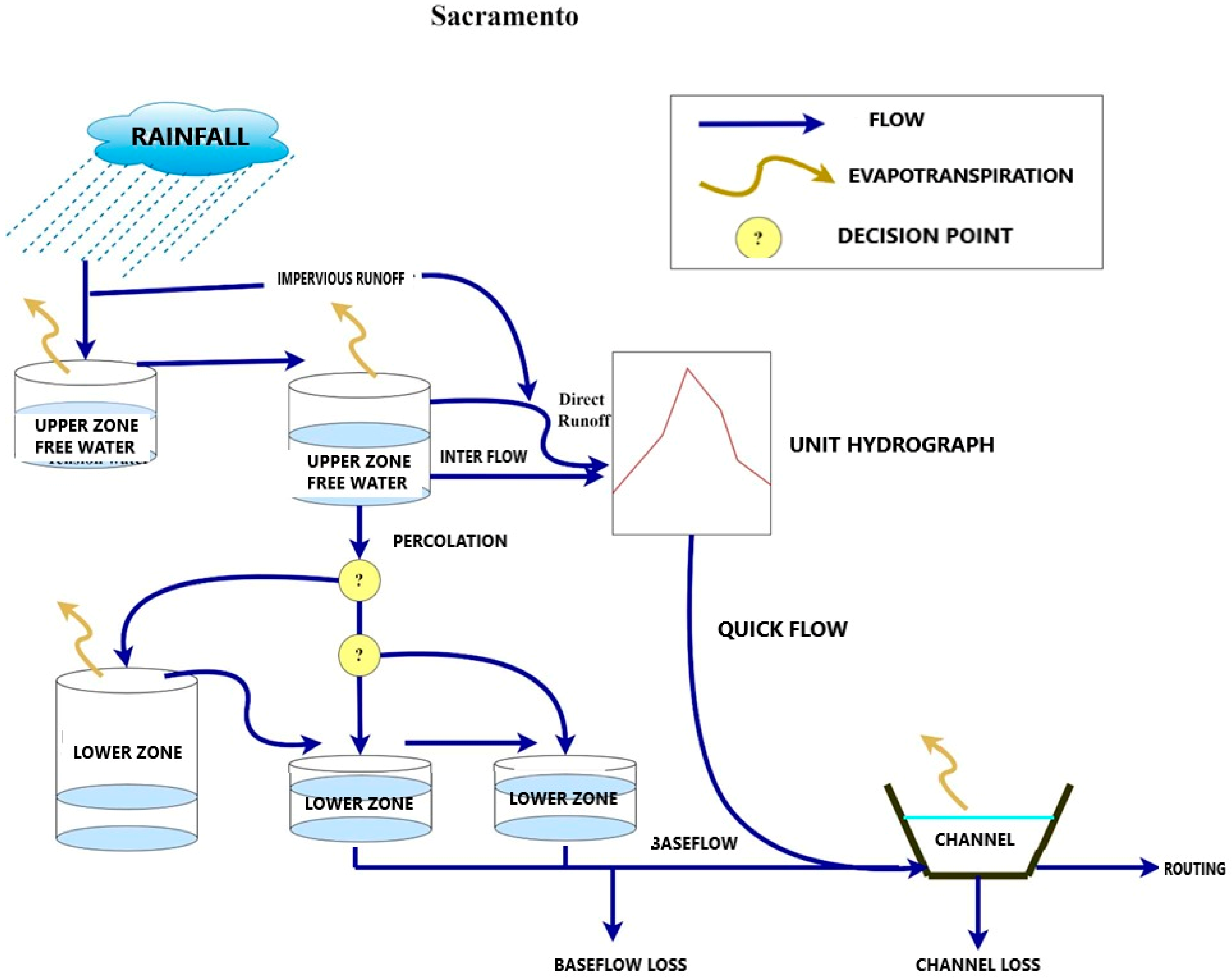
Sacramento
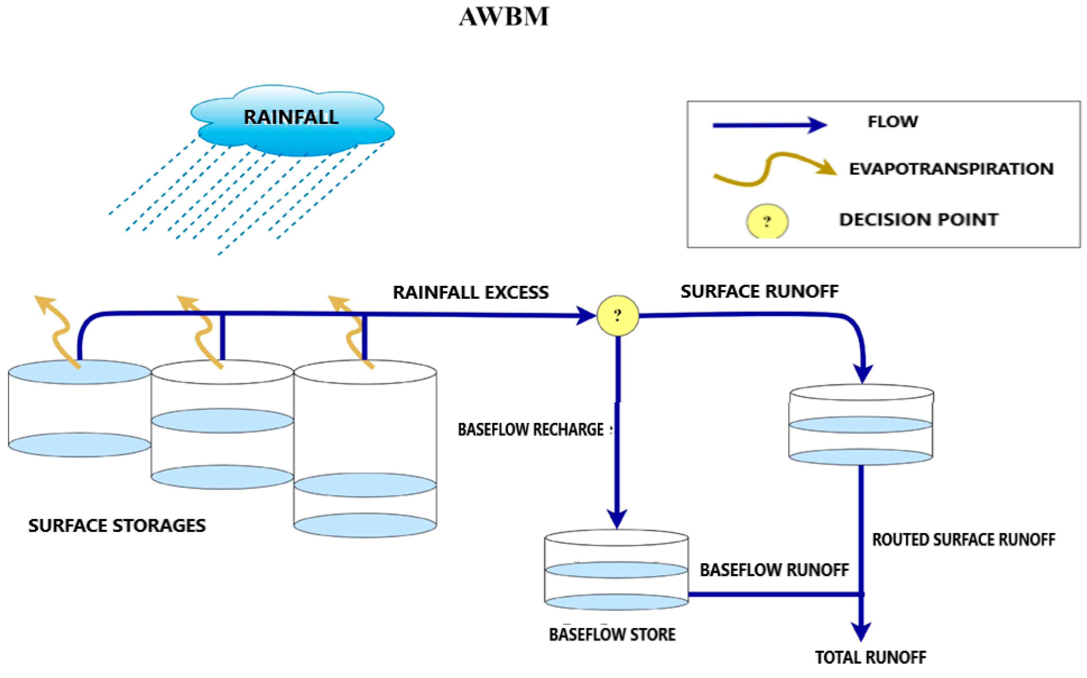
The Australian Water Balance Model
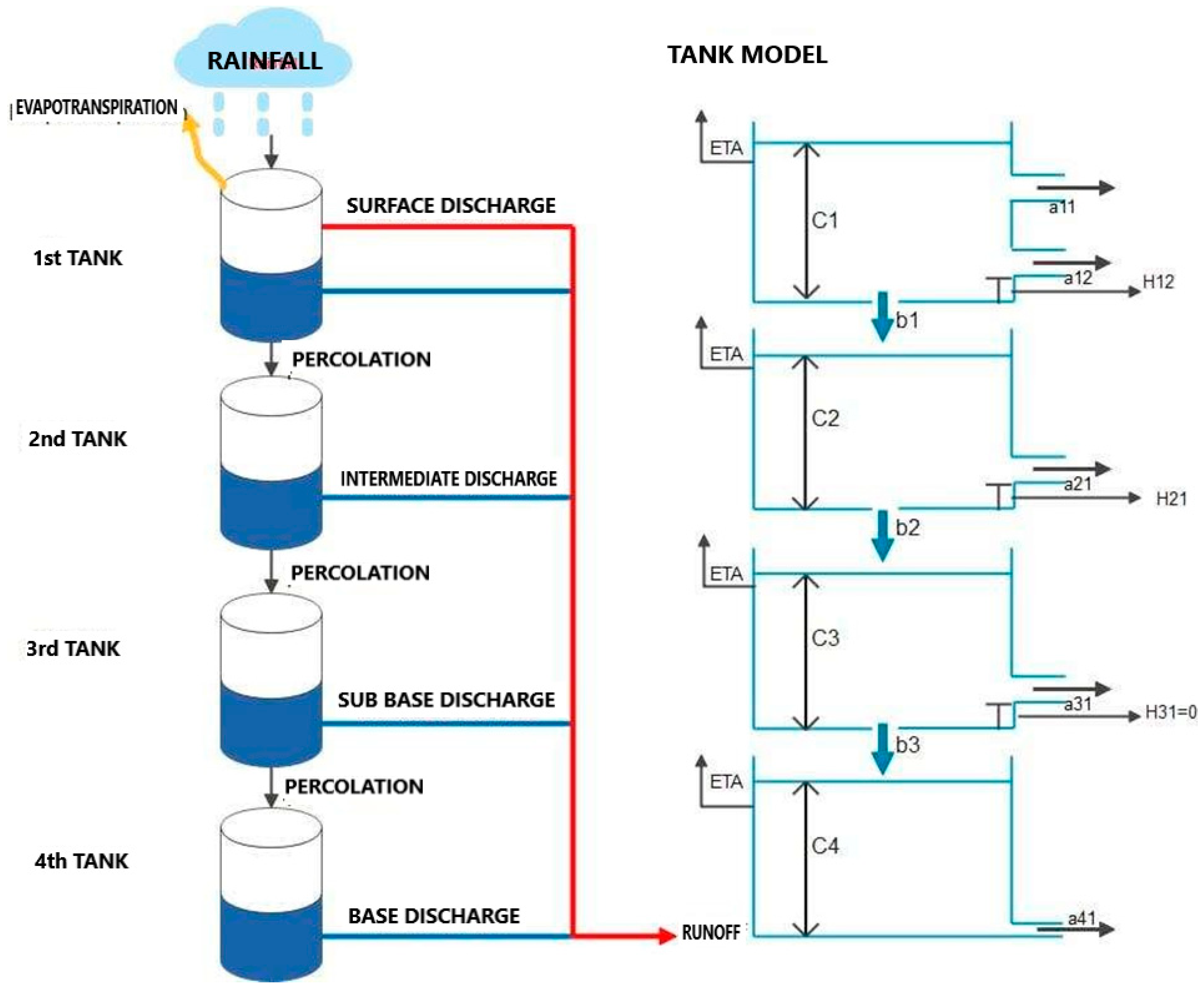
TANK
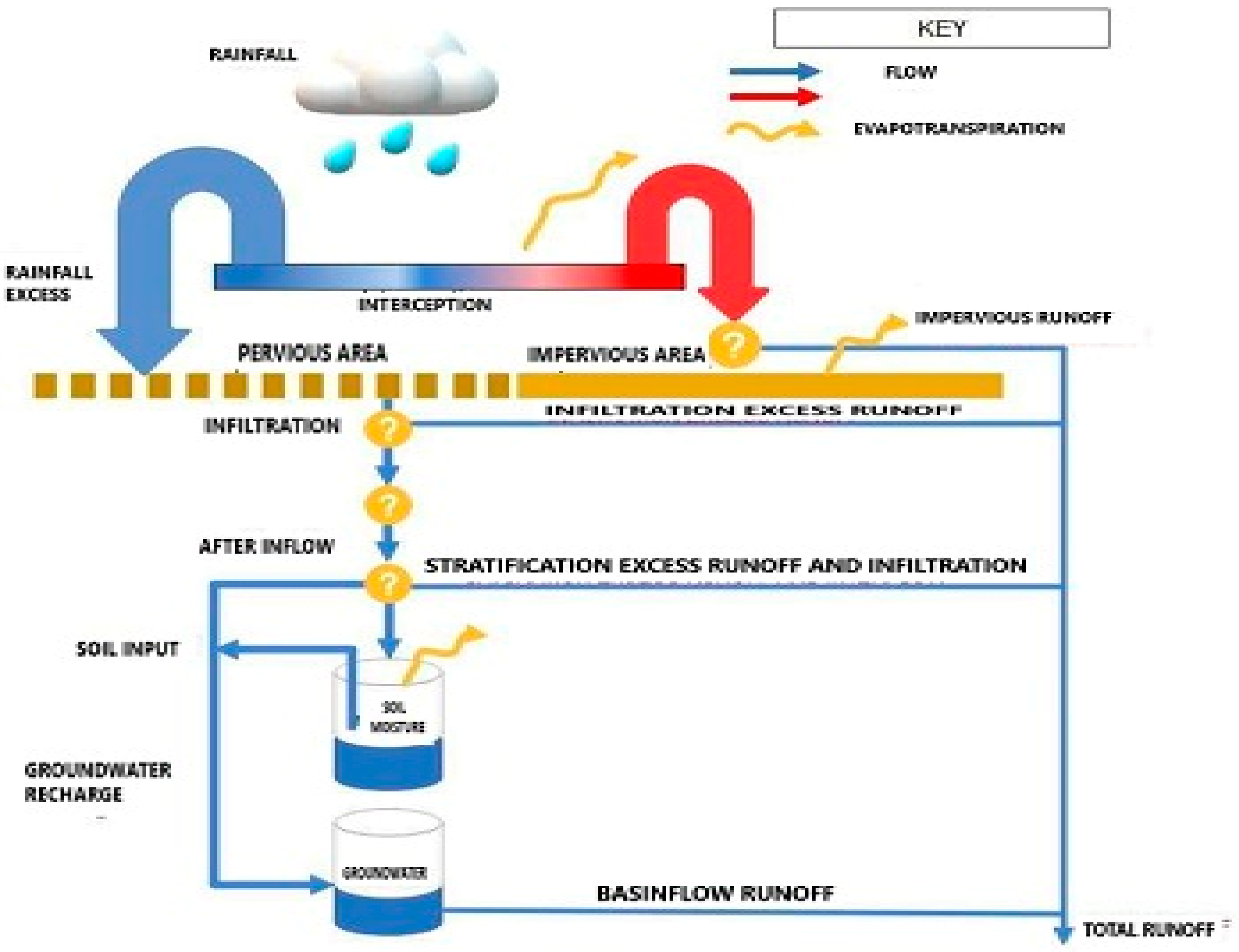
SIMHYD
3. Results and Discussion
3.1. Findings and Talks
3.1.1. Ongoing Metrics Assessment
3.1.2. Evaluation of Categorical Metrics
4. Conclusions
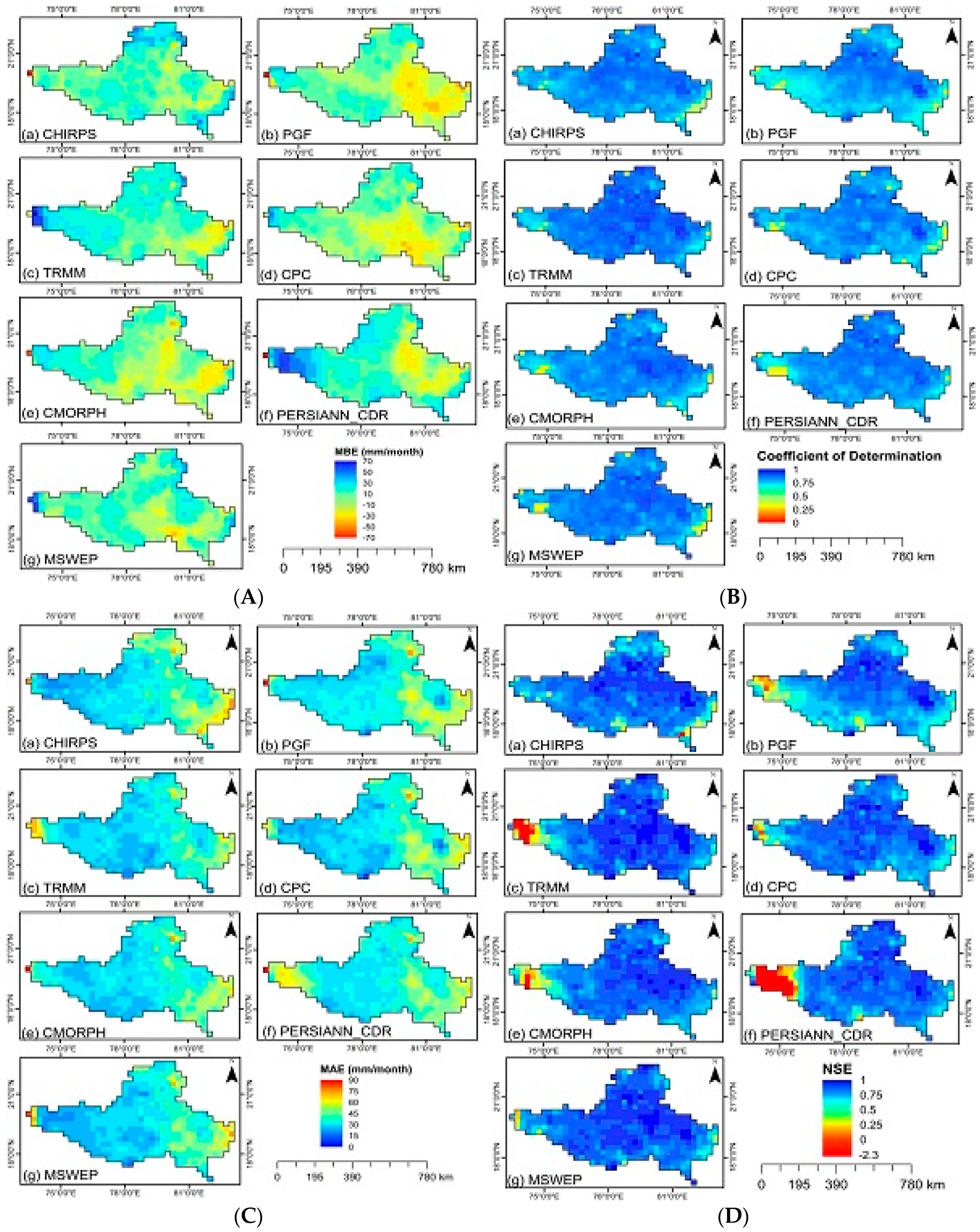
- Geographic Correlation: The satellite precipitation products showed excellent geographic correlation, although the degree of accuracy varied depending on the climate regime and evolving weather patterns influenced by climate change.
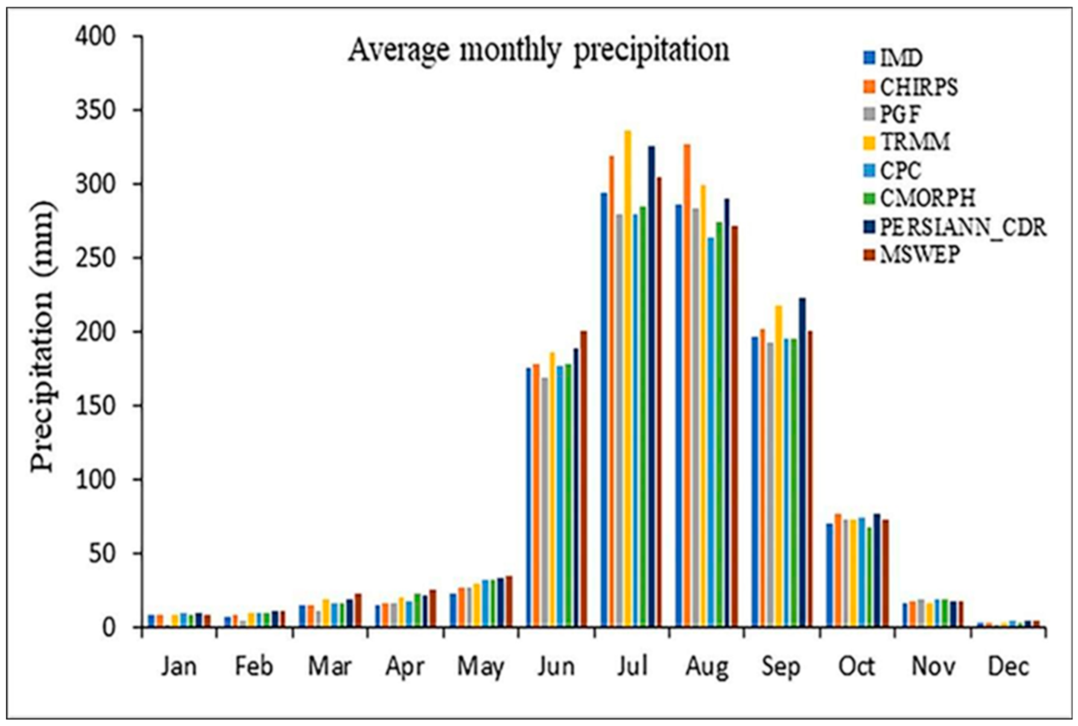
- Monsoon Dominance: The monsoon season (June to September) remains the dominant precipitation period, accounting for approximately 85% of the basin’s total rainfall. This trend aligns with projections of intensified monsoon activities due to climate change, potentially increasing flood risks and altering water resource availability.
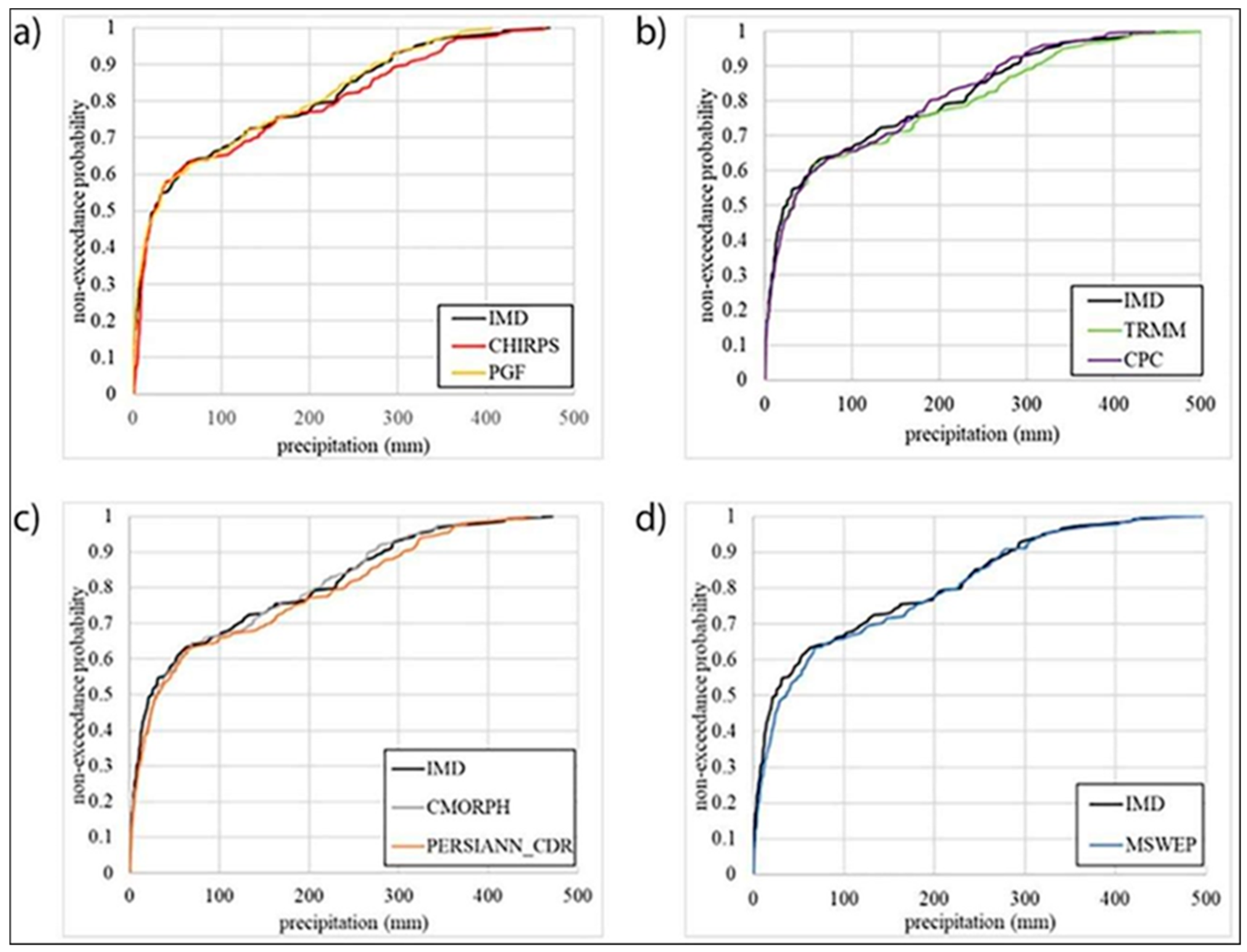
- Seasonal Performance Variations: Except for MSWEP and TRMM, none of the datasets accurately captured precipitation during the pre-monsoon (March–May) and winter (January–February) seasons. This gap is critical under climate change scenarios, where shifts in seasonal precipitation patterns are expected to intensify.
- Performance Under Monsoon and Post-Monsoon Conditions: MSWEP and TRMM outperformed the other datasets during the monsoon and post-monsoon seasons, exhibiting lower Mean Bias Error (MBE), Mean Absolute Error (MAE), and Root Mean Square Error (RMSE), along with higher Nash–Sutcliffe Efficiency (NSE) and coefficient of determination (R2). The MSWEP dataset, in particular, achieved an NSE of 0.806, R2 of 0.831, an MAE of 31.79 mm/month, and an RMSE of 56.73 mm/month, indicating robust performance in tracking precipitation trends amidst climate variability.
- Accuracy in Precipitation Event Detection: MSWEP demonstrated the highest accuracy, with a Peirce’s Skill Score (PSS) of 0.571, a False Alarm Ratio (FAR) of 0.462, and an overall accuracy of 0.844. Additionally, CHIRPS and PERSIANN_CDR successfully detected rainfall occurrences, proving their utility as reliable backup data sources for identifying extreme precipitation events under changing climate conditions.
Author Contributions
Funding
Data Availability Statement
Conflicts of Interest
References
- Agridiotis, V.; Forster, C.F.; Carliell-Marquet, C. Addition of Al and Fe salts during treatment of paper mill effluents to improve activated sludge settlement characteristics. Bioresour. Technol. 2007, 98, 2926–2934. [Google Scholar] [CrossRef] [PubMed]
- Akar, Ö.; Saralioğlu, E.; Güngör, O.; Bayata, H.F. Semantic segmentation of very-high spatial resolution satellite images: A comparative analysis of 3D-CNN and traditional machine learning algorithms for automatic vineyard detection. Int. J. Eng. Geosci. 2024, 9, 12–24. [Google Scholar] [CrossRef]
- Al-Shannag, M.; Al-Qodah, Z.; Bani-Melhem, K.; Qtaishat, M.R.; Alkasrawi, M. Heavy metal ions removal from metal plating wastewater using electrocoagulation: Kinetic study and process performance. Chem. Eng. J. 2015, 260, 749–756. [Google Scholar] [CrossRef]
- Anselmo, L. The long-term evolution of the Italian satellites in the GEO region and their possible interaction with the orbital debris environment. In Proceedings of the 54th International Astronautical Congress of the International Astronautical Federation, the International Academy of Astronautics, and the International Institute of Space Law, Bremen, Germany, 29 September–3 October 2003. IAC-03-IAA.5.2.05. [Google Scholar] [CrossRef]
- Aydın, V.A. Comparison of CNN-based methods for yoga pose classification. Turk. J. Eng. 2024, 8, 65–75. [Google Scholar] [CrossRef]
- Akgül, V.; Görmüş, K.S.; Kutoğlu, Ş.H.; Jin, S. Performance analysis and kinematic test of the BeiDou Navigation Satellite System (BDS) over coastal waters of Türkiye. Adv. Eng. Sci. 2024, 4, 1–14. [Google Scholar]
- Baudhanwala, D.; Mehta, D.; Kumar, V. Machine learning approaches for improving precipitation forecasting in the Ambica River basin of Navsari District, Gujarat. Water Pract. Technol. 2024, 19, 1315–1329. [Google Scholar] [CrossRef]
- Briffa, J.; Sinagra, E.; Blundell, R. Heavy metal pollution in the environment and their toxicological effects on humans. Heliyon 2020, 6, e04691. [Google Scholar] [CrossRef]
- Bakar, A.F.A.; Halim, A.A. Treatment of automotive wastewater by coagulation-flocculation using poly-aluminum chloride (PAC), ferric chloride (FeCl3) and aluminum sulfate (alum). AIP Conf. Proc. 2013, 1571, 524–529. [Google Scholar] [CrossRef]
- Camaj, A.; Haziri, A.; Nuro, A.; Ibrahimi, A.C. Levels of BTEX and Chlorobenzenes in water samples of White Drin River, Kosovo. Adv. Eng. Sci. 2024, 4, 45–53. Available online: https://publish.mersin.edu.tr/index.php/ades/article/view/1326 (accessed on 12 February 2024).
- Capizzi, G.; Lo Sciuto, G.; Napoli, C.; Tramontana, E.; Wozniak, M. Automatic classification of fruit defects based on co-occurrence matrix and neural networks. In Proceedings of the 2015 Federated Conference on Computer Science and Information, Lodz, Poland, 13–16 September 2015; pp. 861–867. [Google Scholar] [CrossRef]
- Çetin Taş, İ.; Bozdoğan, A.M.; Arıca, S. Application of Convolutional Neural Networks for Watermelon Detection in UAV Aerial Images: A Case Study. Turk. J. Eng. 2025, 9, 1–11. [Google Scholar] [CrossRef]
- Chang, S.; Ahmad, R.; Kwon, D.E.; Kim, J. Hybrid ceramic membrane reactor combined with fluidized adsorbents and scouring agents for hazardous metal-plating wastewater treatment. J. Hazard. Mater. 2020, 388, 121777. [Google Scholar] [CrossRef] [PubMed]
- Dursun, S.; Qasim, M.N. Measurements and modelling of PM2.5 level in summertime period in Novada Main Shopping Centre Konya, Turkey. Eng. Appl. 2022, 1, 19–32. Available online: https://publish.mersin.edu.tr/index.php/enap/article/view/314 (accessed on 15 January 2023).
- Demirgül, T.; Yılmaz, C.B.; Zıpır, B.N.; Kart, F.S.; Pehriz, M.F.; Demir, V.; Sevimli, M.F. Investigation of Turkey’s climate periods in terms of precipitation and temperature changes. Eng. Appl. 2022, 1, 80–90. Available online: https://publish.mersin.edu.tr/index.php/enap/article/view/320 (accessed on 18 June 2022).
- Daberdini, A.; Basholli, F.; Metaj, N. Simulation with the Mirone application for the construction of marine mechanical waves generated by possible seismic events in the territory of the Adriatic and Ionian seas. Adv. Eng. Sci. 2023, 3, 46–54. Available online: https://publish.mersin.edu.tr/index.php/ades/article/view/856 (accessed on 13 February 2023).
- Dursun, S.; Sarcan, A. Determination of water quality in Hadim District of Konya (Turkey) and the investigation of disinfection efficiency. Adv. Eng. Sci. 2022, 2, 101–108. Available online: https://publish.mersin.edu.tr/index.php/ades/article/view/89 (accessed on 16 January 2022).
- Ekiz, A.; Arica, S.; Bozdogan, A.M. Classification and Segmentation of Watermelon in Images Obtained by Unmanned Aerial Vehicle. In Proceedings of the ELECO 2019—11th International Conference on Electrical and Electronics Engineering, Bursa, Turkey, 28–30 November 2019; pp. 619–622. [Google Scholar] [CrossRef]
- El Gaayda, J.; Rachid, Y.; Titchou, F.E.; Barra, I.; Hsini, A.; Yap, P.S.; Akbour, R.A. Optimizing removal of chromium (VI) ions from water by coagulation process using central composite design: Effectiveness of grape seed as a green coagulant. Sep. Purif. Technol. 2023, 307, 122805. [Google Scholar] [CrossRef]
- Ezquerro, O.; Ortiz, G.; Pons, B.; Tena, M.T. Determination of benzene, toluene, ethylbenzene and xylenes in soils by multiple headspace solid-phase microextraction. J. Chromatogr. A 2004, 1035, 17–22. [Google Scholar] [CrossRef]
- Fen, İ.Ü.; Enst, B.; Der, K. Kadir SABANCI ve Ark. Available online: http://www.tuik.gov.tr/bitkiselapp/ (accessed on 30 June 2022).
- Fu, S.Y.; Wang, Z.R.; Shi, H.L.; Ma, L.H. The application of decommissioned GEO satellites to CAPS. In Proceedings of the IOP Conference Series: Materials Science and Engineering, Kitakyushu City, Japan, 10–13 April 2018; Volume 372, p. 012033. [Google Scholar] [CrossRef]
- Gangani, P.; Mangukiya, N.K.; Mehta, D.J.; Muttil, N.; Rathnayake, U. Evaluating the efficacy of different DEMs for application in flood frequency and risk mapping of the Indian Coastal River Basin. Climate 2023, 11, 114. [Google Scholar] [CrossRef]
- Gholami, A. Exploring drone classifications and applications: A review. Int. J. Eng. Geosci. 2024, 9, 418–442. [Google Scholar] [CrossRef]
- Gordani, O.; Simoni, A. Leveraging SVD for efficient image compression and robust digital watermarking. Adv. Eng. Sci. 2024, 4, 103–112. Available online: https://publish.mersin.edu.tr/index.php/ades/article/view/1496 (accessed on 3 September 2024).
- Gohil, M.; Mehta, D.; Shaikh, M. An integration of geospatial and fuzzy-logic techniques for multi-hazard mapping. Results Eng. 2024, 21, 101758. [Google Scholar] [CrossRef]
- Hosseini, S.S.; Bringas, E.; Tan, N.R.; Ortiz, I.; Ghahramani, M.; Shahmirzadi, M.A.A. Recent progress in development of high performance polymeric membranes and materials for metal plating wastewater treatment: A review. J. Water Process Eng. 2016, 9, 78–110. [Google Scholar] [CrossRef]
- Huang, J.; Yuan, F.; Zeng, G.; Li, X.; Gu, Y.; Shi, L.; Liu, W.; Shi, Y. Influence of pH on heavy metal speciation and removal from wastewater using micellar-enhanced ultrafiltration. Chemosphere 2017, 173, 199–206. [Google Scholar] [CrossRef] [PubMed]
- Ilhan, F.; Ulucan-Altuntas, K.; Avsar, Y.; Kurt, U.; Saral, A. Electrocoagulation process for the treatment of metal-plating wastewater: Kinetic modeling and energy consumption. Front. Environ. Sci. Eng. 2019, 13, 1–8. [Google Scholar] [CrossRef]
- Kocalar, A.C. Sinkholes caused by agricultural excess water using and administrative traces of the process. Adv. Eng. Sci. 2023, 3, 15–20. Available online: https://publish.mersin.edu.tr/index.php/ades/article/view/756 (accessed on 18 January 2023).
- Kalay, E.; Sarıoğlu, H.; Özkul, I. Design parameters of sand filtration systems in wastewater treatment process. Adv. Eng. Sci. 2021, 1, 34–42. Available online: https://publish.mersin.edu.tr/index.php/ades/article/view/23 (accessed on 24 August 2021).
- Mehta, D.; Prajapati, K.; Islam, M.N. Watershed delineation and land use land cover (LULC) study of Purna River in India. In India II: Climate Change Impacts, Mitigation and Adaptation in Developing Countries; Springer International Publishing: Cham, Switzerland, 2021; pp. 169–181. [Google Scholar]
- Mukasa, P.; Wakoli, C.; Faqeerzada, M.A.; Amanah, H.Z.; Kim, H.; Joshi, R.; Suh, H.K.; Kim, J.; Lee, H.; Kim, M.S.; et al. Nondestructive discrimination of seedless from seeded watermelon seeds by using multivariate and deep learning image analysis. Comput. Electron. Agric. 2022, 194, 106799. [Google Scholar] [CrossRef]
- Mehta, D.; Hadvani, J.; Kanthariya, D.; Sonawala, P. Effect of land use land cover change on runoff characteristics using curve number: A GIS and remote sensing approach. Int. J. Hydrol. Sci. Technol. 2023, 16, 1–16. [Google Scholar] [CrossRef]
- Reddy, N.M.; Saravanan, S.; Almohamad, H.; Al Dughairi, A.A.; Abdo, H.G. Effects of Climate Change on Streamflow in the Godavari Basin Simulated Using a Conceptual Model including CMIP6 Dataset. Water 2023, 15, 1701. [Google Scholar] [CrossRef]
- Nguyen, M.K.; Tran, V.S.; Pham, T.T.; Pham, H.G.; Hoang, B.L.; Nguyen, T.H.; Nguyen, T.H.; Tran, T.H.; Ngo, H.H. Fenton/ozone-based oxidation and coagulation processes for removing metals (Cu, Ni)-EDTA from plating wastewater. J. Water Process Eng. 2021, 39, 101836. [Google Scholar] [CrossRef]
- Oymak, A.; Tür, M.R.; Bouchiba, N. PV connected pumped-hydro storage system. Eng. Appl. 2022, 1, 46–54. Available online: https://publish.mersin.edu.tr/index.php/enap/article/view/316 (accessed on 18 June 2022).
- Öz, İ.; Yılmaz, Ü.C. Determination of coverage oscillation for inclined communication satellite. Sak. Univ. J. Sci. 2020, 24, 973–983. [Google Scholar] [CrossRef]
- Oz, I. Salınımlı yörünge haberleşme uydularında 2 eksen düzeltmeli kapsama alanı stabilizasyonu. J. Fac. Eng. Archit. Gazi Univ. 2022, 38, 219–229. [Google Scholar] [CrossRef]
- Palansooriya, K.N.; Yang, Y.; Tsang, Y.F.; Sarkar, B.; Hou, D.; Cao, X.; Meers, E.; Rinklebe, J.; Kim, K.H.; Ok, Y.S. Occurrence of contaminants in drinking water sources and the potential of biochar for water quality improvement: A review. Crit. Rev. Environ. Sci. Technol. 2020, 50, 549–611. [Google Scholar] [CrossRef]
- Pfaff, K.; Hildebrandt, L.H.; Leach, D.L.; Jacob, D.E.; Markl, G. Formation of the Wiesloch Mississippi Valley-type Zn-Pb-Ag deposit in the extensional setting of the Upper Rhinegraben, SW Germany. Miner. Deposita 2010, 45, 647–666. [Google Scholar] [CrossRef]
- Qasem, N.A.; Mohammed, R.H.; Lawal, D.U. Removal of heavy metal ions from wastewater: A comprehensive and critical review. Npj Clean Water 2021, 4, 36. [Google Scholar] [CrossRef]
- Raaj, S.; Gupta, V.; Singh, V.; Shukla, D.P. A novel framework for peak flow estimation in the Himalayan river basin by integrating SWAT model with machine learning based approach. Earth Sci. Inform. 2024, 17, 211–226. [Google Scholar] [CrossRef]
- Sattari, M.T.; Kamrani, Y.; Javidan, S.; Fathollahzadeh Attar, N.; Apaydın, H. Groundwater quality mapping based on the Wilcox Classification method for agricultural purposes: Qazvin Plain aquifer case. Turk. J. Eng. 2025, 9, 116–128. [Google Scholar] [CrossRef]
- Salamon, J.; Bello, J.P. Deep Convolutional Neural Networks and Data Augmentation for Environmental Sound Classification. IEEE Signal Process. Lett. 2017, 24, 279–283. [Google Scholar] [CrossRef]
- Tchounwou, P.B.; Yedjou, C.G.; Patlolla, A.K.; Sutton, D.J. Heavy metal toxicity and the environment. In Molecular, Clinical and Environmental Toxicology: Volume 3: Environmental Toxicology; Springer: Berlin/Heidelberg, Germany, 2012; Volume 3, pp. 133–164. [Google Scholar] [CrossRef]
- Verma, S.; Verma, M.K.; Prasad, A.D.; Mehta, D.; Azamathulla, H.M.; Muttil, N.; Rathnayake, U. Simulating the hydrological processes under multiple land use/land cover and climate change scenarios in the mahanadi reservoir complex, Chhattisgarh, India. Water 2023, 15, 3068. [Google Scholar] [CrossRef]
- Verma, S.; Kumar, K.; Verma, M.K.; Prasad, A.D.; Mehta, D.; Rathnayake, U. Comparative analysis of CMIP5 and CMIP6 in conjunction with the hydrological processes of reservoir catchment, Chhattisgarh, India. J. Hydrol. Reg. Stud. 2023, 50, 101533. [Google Scholar] [CrossRef]
- Verma, S.; Verma, M.K.; Prasad, A.D.; Mehta, D.J.; Islam, M.N. Modeling of uncertainty in the estimation of hydrograph components in conjunction with the SUFI-2 optimization algorithm by using multiple objective functions. Model. Earth Syst. Environ. 2024, 10, 61–79. [Google Scholar] [CrossRef]
- Wan Nurazwin Syazwani, R.; Muhammad Asraf, H.; Megat Syahirul Amin, M.A.; Nur Dalila, K.A. Automated image identification, detection and fruit counting of top-view pineapple crown using machine learning. Alex. Eng. J. 2022, 61, 1265–1276. [Google Scholar] [CrossRef]
- Witkowska, D.; Słowik, J.; Chilicka, K. Heavy metals and human health: Possible exposure pathways and the competition for protein binding sites. Molecules 2021, 26, 6060. [Google Scholar] [CrossRef] [PubMed]
- Yalçın, C.; Canlı, H. IP/Resistivity methods for Pb-Zn deposit exploration: A case study in Sudöşeği, (Simav-Kütahya, Türkiye). Eng. Appl. 2024, 3, 27–35. Available online: https://publish.mersin.edu.tr/index.php/enap/article/view/1503 (accessed on 15 February 2024).
- Yalçın, C. Geochemical and geological approach to the carbonate-hosted barite deposits in Dadağlı (Kahramanmaraş), Turkey. Eng. Appl. 2022, 1, 55–62. Available online: https://publish.mersin.edu.tr/index.php/enap/article/view/317 (accessed on 19 June 2022).
- Yoshioka, K.; Zhdanov, M.S. Three-dimensional nonlinear regularized inversion of the induced polarization data based on the Cole–Cole model. Phys. Earth Planet. Inter. 2005, 150, 29–43. [Google Scholar] [CrossRef]
- Zamora-Ledezma, C.; Negrete-Bolagay, D.; Figueroa, F.; Zamora-Ledezma, E.; Ni, M.; Alexis, F.; Guerrero, V.H. Heavy metal water pollution: A fresh look about hazards, novel and conventional remediation methods. Environ. Technol. Innov. 2021, 22, 101504. [Google Scholar] [CrossRef]
- Zhu, Y.; Fan, W.; Zhou, T.; Li, X. Removal of chelated heavy metals from aqueous solution: A review of current methods and mechanisms. Sci. Total Environ. 2019, 678, 253–266. [Google Scholar] [CrossRef]


| Model | Atmospheric Resolution | Institution |
|---|---|---|
| ACCESS-ESM1-5 | 1.9° × 1.2° | The Commonwealth Scientific and Industrial Research Organization (CSIRO) and the Australian Bureau of Meteorology |
| ACCESS-CM2 | 1.87° × 1.25° | The Commonwealth Scientific and Industrial Research Organization (CSIRO) and the Australian Bureau of Meteorology (BOM) |
| CanESM5 | 2.81° × 2.79° | Canada’s Centre for Climate Modelling and Analysis, The Centre for Climate Change in Europe and the Mediterranean |
| EC-Earth3 | 1.3° × 0.9° | Consortium EC-EARTH |
| EC-Earth3-Veg | 0.7° × 0.7° | Consortium EC-EARTH |
| EC-Earth3-Veg-LR | 0.7° × 0.7° | Consortium EC-EARTH |
| GFDL-ESM4 | 1.1° × 1.1° | Geophysical Fluid Dynamics Laboratory |
| INM-CM5-0 | 1.3° × 1° | The Institute of Numerical Mathematics |
| IPSL-CM6A-LR | 2° × 1.5° | Institute of Pierre-Simon Laplace |
| MIROC6 | 1.41° × 1.41° | R-CCS, AORI, NIES, and JAMSTEC |
| MPI-ESM1-2-HR | 0.93° × 0.93° | The Max Planck Institute of Meteorology (MPI-M) |
| MPI-ESM1-2-LR | 0.93° × 0.93° | The Max Planck Institute of Meteorology (MPI-M) |
| MRI-ESM2-0 | 0.9° × 1.3° | Meteorological Research Institute |
| NorESM2-LM | 0.9° × 1.3° | Meteorological Research Institute |
| NorESM2-MM | 1.3° × 1° | The Taiwan Earth System Model, Version 1 |
| Parameter | Description | Default | Min | Max |
|---|---|---|---|---|
| LZPK | The proportion of water in LZFPM that drains daily as base flow. | Zone | Free | Water |
| LZSK | The proportion of water in LZFSM that drains daily as base flow. | 60 | 40 | 600 |
| UZK | The percentage of water in UZFWM that drains as daily interflow. | 0.06 | 0 | 0.5 |
| UZTWM | Maximum Water Tension in the Upper Zone. | 1 | 0 | 3 |
| UZFWM | The storage that serves as the source of water for interflow and the impetus for moving water to greater depths is known as the Upper Zone Free Water Maximum. | 40 | 0 | 80 |
| LZTWM | Water Maximum for Lower Zone Tension. | 0 | 0 | 0.8 |
| LZFSM | Maximum Free Water Supplement in the Lower Zone. | 0.01 | 0.001 | 0.015 |
| LZFPM | Primary Maximum for Lower Zone Free Water. | 0.05 | 0.03 | 0.2 |
| PFREE | Recharging the lower zone’s free water reservoirs requires a minimum percentage of percolation from the upper zone to the lower zone. | 0.3 | 0.2 | 0.5 |
| REXP | An exponent that calculates how quickly the percolation rate changes as the lower zone water storage changes | 50 | 25 | 125 |
| ZPERC | The maximal percolation rate is determined by the proportionate increase in Pbase | 40 | 10 | 75 |
| SIDE | The non-channel base flow ratio. | 130 | 75 | 300 |
| Parameter | Description | Default | Min | Max |
|---|---|---|---|---|
| KSurf | Recession constant of surface flow | 150 | 0 | 500 |
| KBase | Recession constant for base flow | 70 | 0 | 200 |
| C3 | Surface store capacity 3 (in mm) | 7 | 0 | 50 |
| C2 | Surface store capacity 2 (in mm) | 0.35 | 0 | 1 |
| C1 | Surface store capacity 1 (in mm) | 0.95 | 0 | 1 |
| BFI | Index of base flow | 0.134 | 0 | 1 |
| A2 | Surface storage 2’s partial area | 0.35 | 0 | 1 |
| A1 | Surface store 1’s partial area | 0.35 | 0 | 1 |
| KSurf | Recession constant of surface flow | 0.433 | 0 | 1 |
| Parameter | Minimum | Default Value | Maximum |
|---|---|---|---|
| First outlet height of the first tank (H11) (in mm) | 0 | 0 | 500 |
| Second outlet height of first tank (H12) (in mm) | 0 | 0 | 300 |
| First outlet height of the second, third, and fourth tanks (H21, H31, and H41) (in mm) | 0 | 0 | 100 |
| Coefficient of runoff from various tank outlets (a11, a12, a21, a31, and a41) | 0 | 0.2 | 1 |
| Coefficient of Evaporation (α) | 0 | 0.1 | 1 |
| Coefficient of infiltration in tanks 1, 2, and 3 (b1, b2, and b3) | 0 | 0.2 | 1 |
| Tank’s water level (C1, C2, C3, and C4) (in mm) | 0 | 20 | 100 |
| Parameter | Minimum | Default Value | Maximum |
|---|---|---|---|
| Baseflow coefficient | 0.0 | 0.9 | 1.0 |
| Unaffected Threshold | 0.0 | 1.5 | 5.0 |
| Infiltration Coefficient | 0.0 | 0.2 | 1.0 |
| Infiltration Form | 1 | 320 | 500 |
| Interflow Coefficient | 0.0 | 0.3 | 1.0 |
| Prior Fraction | 0 | 1 | 5 |
| Capacity of the Rainfall Interception Store | 0 | 200 | 400 |
| Recharge Coefficient | 0 | 3 | 10 |
| Soil Moisture Store Capacity | 0.0 | 0.1 | 1.0 |
| DATA | Temporal Resolution | Availability | Link |
|---|---|---|---|
| IMD | 0.25° and D | 1951–2024 | The website https://www.imdpune.gov.in/, accessed on 7 April 2025 |
| CHIRPS | 0.05° and D and M | 1981–present | CHIRPS 2.0: https://data.chc.ucsb.edu/products/, accessed on 7 April 2025 |
| PGF | 0.25° and D | 1948–2020 | https://hydrology.soton.ac.uk/, accessed on 7 April 2025 |
| TRMM | 0.25° and 3H, D and M | 1998–2023 | The summary can be seen at https://disc.gsfc.nasa.gov/datasets/TRMM_3B42_Daily_7, accessed on 7 April 2025 |
| CPC | 0.5° and D | 1979–present | Balprecip.html https://psl.noaa.gov/data/gridded/data.cpc.glo, accessed on 7 April 2025 |
| CMORPH | 0.25° and 30 min, 1H and D | 1998–2024 | https://www.ncei.noaa.gov/products/climate-data-records, accessed on 7 April 2025 |
| PERSIA NN_CDR | 0.25° and D and M | 1983–Present | https://chrsdata.eng.uci.edu/, accessed on 7 April 2025 |
| MSWEP | 0.1° and 3H, D and M | 1979–2024 | Gloh2o.org/mswep/’s website |
| DATA | NSE | R2 | MBE | MAE | RMSE |
|---|---|---|---|---|---|
| CHIRPS | 0.768 | 0.812 | 7.505 | 34.324 | 61.519 |
| PGF | 0.72 | 0.768 | −2.433 | 35.502 | 66.775 |
| TRMM | 0.768 | 0.846 | 9.126 | 31.528 | 57.413 |
| CPC | 0.772 | 0.801 | −0.774 | 33.247 | 61.58 |
| CMORPH | 0.767 | 0.815 | 0.157 | 32.663 | 60.16 |
| PERSIANN_CDR | 0.667 | 0.815 | 9.332 | 35.934 | 65.177 |
| MSWEP | 0.806 | 0.831 | 5.531 | 31.794 | 56.734 |
| Sacramento | AWBM | TANK | SIMHYD |
|---|---|---|---|
| ADIM 0.031 | A1 0.014 | H11 119.60 | base flow Coefficient 0.373 |
| LZFP 49.608 | A2 0.433 | a11 0.169 | Impervious Threshold 4.431 |
| LZFS M 49.608 | BFI 0.298 | a12 0.204 | Infiltration Coefficient 371.76 |
| LZPK 0.118 | C1 1.569 | a21 0.812 | Infiltration Shape 0.196 |
| LZSK 0.729 | C2 130.1 96 | a31 0.847 | Interflow Coefficient 0.000 |
| LZTW M 117.647 | C3 252.9 41 | a41 0.478 | previous Fraction 1.000 |
| PCTI M 0.000 | KBase 0.561 | alpha 1.000 | rainfall Interception Capacity 4.569 |
| PFREE 0.184 | KSurf 0.627 | b1 0.031 | Recharge Coefficient 0.741 |
| REXP 1.529 | b2 0.337 | Soil Moisture Store Capacity 169.29 0 | |
| RSERV 0.300 | b3 0.027 | ||
| SARVA 0.010 | C1 51.765 | ||
| SIDE 0.000 | C2 18.824 | ||
| SSOUT 0.001 | C3 52.549 | ||
| UZFWM 79.373 | C4 26.667 |
Disclaimer/Publisher’s Note: The statements, opinions and data contained in all publications are solely those of the individual author(s) and contributor(s) and not of MDPI and/or the editor(s). MDPI and/or the editor(s) disclaim responsibility for any injury to people or property resulting from any ideas, methods, instructions or products referred to in the content. |
© 2025 by the authors. Licensee MDPI, Basel, Switzerland. This article is an open access article distributed under the terms and conditions of the Creative Commons Attribution (CC BY) license (https://creativecommons.org/licenses/by/4.0/).
Share and Cite
Ande, R.; Pandugula, C.; Mehta, D.; Vankayalapati, R.; Birbal, P.; Verma, S.; Azamathulla, H.M.; Nanavati, N. Understanding Climate Change Impacts on Streamflow by Using Machine Learning: Case Study of Godavari Basin. Water 2025, 17, 1171. https://doi.org/10.3390/w17081171
Ande R, Pandugula C, Mehta D, Vankayalapati R, Birbal P, Verma S, Azamathulla HM, Nanavati N. Understanding Climate Change Impacts on Streamflow by Using Machine Learning: Case Study of Godavari Basin. Water. 2025; 17(8):1171. https://doi.org/10.3390/w17081171
Chicago/Turabian StyleAnde, Ravi, Chandrashekar Pandugula, Darshan Mehta, Ravikumar Vankayalapati, Prashant Birbal, Shashikant Verma, Hazi Mohammad Azamathulla, and Nisarg Nanavati. 2025. "Understanding Climate Change Impacts on Streamflow by Using Machine Learning: Case Study of Godavari Basin" Water 17, no. 8: 1171. https://doi.org/10.3390/w17081171
APA StyleAnde, R., Pandugula, C., Mehta, D., Vankayalapati, R., Birbal, P., Verma, S., Azamathulla, H. M., & Nanavati, N. (2025). Understanding Climate Change Impacts on Streamflow by Using Machine Learning: Case Study of Godavari Basin. Water, 17(8), 1171. https://doi.org/10.3390/w17081171