Abstract
Understanding the spatiotemporal dynamics of short-duration heavy rainfall (SDHR) is critical for urban flood management. This study applies the K-shape clustering algorithm to classify 105 SDHR events in Beijing (2009–2021) using hourly rainfall data. Compared to K-means and DTW, K-shape prioritizes temporal shape alignment, crucial for capturing phase-shifted rainfall patterns. Three clusters emerged: (1) localized moderate-intensity events (13.3% of events) peaking at noon (11:00–14:00 LST) in western/southeastern regions, with weak burstiness (44.3% stations peak within 0–1 h) and moderate spatial variability (Cv = 1.08); (2) highly variable, intense urban rainfall (47.6% of events) characterized by rapid burstiness (72.5% stations peak within 0–1 h) and extreme spatial heterogeneity (Cv = 1.21), concentrated in central urban areas with peak intensities >130 mm/h; (3) prolonged heavy rainfall (39.1% of events) lasting >6 h, featuring significant accumulation (mean > 50 mm/day) in northeastern plains. The framework identifies high-risk zones (e.g., Cluster 2’s urban flash floods) and informs adaptive drainage design (e.g., prolonged resilience for Cluster 3). This study highlights the necessity of combining statistical metrics with domain expertise for robust SDHR classification and provides insights for urban flood management, emphasizing targeted strategies for different rainfall patterns.
1. Introduction
Short-duration heavy rainfall (SDHR) events, exacerbated by global climate change, pose significant risks to urban areas, leading to flooding, waterlogging, and landslides. Observations indicate a 2% annual increase in SDHR intensity, with a 14% enhancement per °C rise in temperature due to increased atmospheric moisture-holding capacity [1,2]. Urban and mountainous regions are particularly vulnerable due to the urban heat island effect and topographical influences, with frequency and intensity expected to rise [3,4,5,6]. The devastating 2018 event in China, which affected over 35 million people and caused economic losses exceeding RMB 100 billion, exemplifies the growing impacts of extreme rainfall [7,8]. A particularly striking case is the 31 July 2018 Hami rainstorm in Xinjiang, which recorded 110 mm of rainfall within just one hour—more than twice the local annual mean—triggering flash floods, reservoir collapse, and 20 fatalities [9]. Given the strong correlation between SDHR characteristics (intensity, duration, frequency, and spatial distribution) and flood severity [10,11,12], a comprehensive understanding of its spatiotemporal patterns is critical for improving flood mitigation strategies, urban drainage planning, and disaster preparedness.
SDHR events can be classified into distinct patterns based on their spatial and temporal characteristics, as they exhibit significant variability in both their temporal burstiness and spatial heterogeneity. Identifying these patterns is crucial, as different types of SDHR may lead to varying degrees of localized flooding [13,14,15,16]. For instance, Lei et al. [17] classified extreme rainfall in Shanghai, revealing distinct hotspots in eastern suburbs with unique spatiotemporal signatures. Analyzing the common characteristics within each pattern allows for more accurate flood risk predictions and the development of targeted flood mitigation strategies [18,19,20]. By understanding these classification-based patterns, urban planners can better anticipate high-risk areas and optimize infrastructure planning, such as drainage systems and flood barriers.
Classification of SDHR events traditionally relies on three main methodologies: threshold-based approaches, frequency analysis, and atmospheric dynamics methods. Threshold-based methods utilize predefined intensity duration criteria (e.g., hourly rainfall rates exceeding 20, 30, or 50 mm/h), enabling rapid assessment for disaster response [21,22]. Frequency analysis employs statistical distributions like Gumbel and Weibull to estimate rainfall return periods from historical data, facilitating urban infrastructure planning and flood risk assessment [23]. Atmospheric dynamics approaches classify rainfall based on physical formation processes, distinguishing between convective and stratiform systems and providing deeper meteorological insights [24]. However, traditional methods face critical limitations: threshold-based approaches overlook localized rainfall variability; frequency analysis often inaccurately assumes climate stationarity [25]; and atmospheric dynamics methods require extensive datasets and high computational resources, limiting real-time applicability. Moreover, they struggle with large datasets, complex spatiotemporal dependencies, and extreme events analysis. Extensive data preprocessing is also required to reconstruct spatiotemporal rainfall processes, restricting their ability to capture the dynamic nature of SDHR events.
To address these limitations, advancements in computational technology have spurred the exploration of more advanced data analysis techniques, particularly in the realm of unsupervised learning. As a subset of machine learning, unsupervised learning excels at autonomously detecting patterns within unlabeled data, making it highly suitable for analyzing complex meteorological datasets [26,27]. Clustering algorithms, a key component of unsupervised learning, group data based on similar characteristics, revealing underlying structures and patterns [28,29]. These methods have demonstrated significant potential in classifying meteorological data and identifying SDHR events. For instance, studies have applied unsupervised learning to classify rainfall types in various regions, explore the relationship between rainfall timing patterns and flood types, and group standardized rainfall profiles, identifying distinct clusters with varying rainfall intensities and patterns [14,30,31].
Among clustering algorithms, the K-means algorithm is widely used for classifying precipitation events due to its simplicity and efficiency [32,33,34,35]. However, K-means faces three critical challenges in SDHR classification: (1) sensitivity to temporal phase shifts (e.g., rainfall peaks occurring early vs. late in storms) due to Euclidean distance limitations; (2) bias toward absolute intensity differences (e.g., 50 mm/h vs. 30 mm/h events with identical temporal shapes); and (3) dimensionality reduction requirements (e.g., PCA) that discard spatiotemporal features [36,37,38]. To overcome these challenges, the K-shape clustering algorithm has emerged as a promising alternative. Unlike K-means, K-shape groups data based on the similarity in the shape of time series, making it more suitable for analyzing SDHR data [39,40]. Although K-shape has been underexplored in rainfall classification, it has shown success in other fields, such as energy consumption, passenger flow, and medical signal analysis [41,42,43,44]. These applications demonstrate its potential for handling spatiotemporal data effectively.
This study examines SDHR events in Beijing, where rainfall intensity increased by 18% from 1961 to 2021 despite frequency fluctuations. This trend is influenced by the region’s complex topography (Taihang-Yan Mountains), urban heat island effects, and mesoscale systems such as the Huang-Huai low-pressure vortex [45,46,47]. A notable example is the 2012 “7·21” event, which delivered 460 mm of rainfall in 18 h, paralyzing transportation and causing 79 fatalities [48]. Sun’s research identifies two predominant SDHR types that are based on an atmospheric dynamics approach: one with lower daily rainfall but intense, localized downpours, and another with higher daily totals, longer duration, and broader spatial distribution [49]. Most previous studies have predominantly used daily precipitation data, which fails to capture the fine-scale temporal and spatial characteristics of SDHR. Recent research has shown that higher-resolution hourly precipitation data provide more insights into the burstiness and locality of SDHR events [50,51,52]. Therefore, this study analyzes 105 SDHR events in Beijing using high-resolution hourly data (2009–2021) and classifies them with the K-shape algorithm. By comparing these results with traditional methods, we address three key gaps: (1) spatiotemporal heterogeneity across clusters, (2) algorithmic limitations of traditional approaches, and (3) practical implications for flood forecasting and infrastructure design. These insights will help identify high-risk areas most vulnerable to SDHR events, improve forecasting accuracy, and optimize flood control strategies.
The objective of this study is to apply the K-shape clustering algorithm to classify SDHR events in Beijing and analyze their spatiotemporal characteristics. Specifically, this study aims to identify differences in spatiotemporal patterns across different rainfall types and explore their relationships with mesoscale circulation features. The methodology involves using high-resolution hourly precipitation data and the K-shape algorithm to classify rainfall events based on their spatiotemporal features. The structure of the paper is as follows: Section 2 presents the methodology, including data sources, the clustering approach, and spatial feature analysis; Section 3 presents the clustering results and analyzes the spatiotemporal distribution patterns of different rainfall types; Section 4 discusses the implications of these patterns for urban flood management and drainage systems; and Section 5 summarizes the study’s findings, highlights its strengths and weaknesses, and suggests directions for future research.
2. Materials and Methods
2.1. Study Area and Datasets
Beijing, the capital of China, is located in the northern part of the North China Plain, between longitudes 115°41′ and 117°50′ and latitudes 39°44′ and 41°05′, covering an area of approximately 16,400 square kilometers. The city is surrounded by the Taihang and Yanshan Mountains to the west and north, which force moist air upward, leading to increased extreme rainfall in windward areas, particularly in the northeastern and southwestern mountainous regions [47,53]. In addition, Beijing experiences a temperate monsoon climate with semi-humid and semi-arid characteristics, influenced by various weather systems, including the westerly trough, northeastern cold vortex, and the Huang-Huai low-pressure system [20,54,55]. Synoptic-scale systems trigger and enhance vertical convective motion through local convergence-lifting mechanisms. Their combined effects—including the superposition of upward airflows and intensified water vapor convergence—drive extreme short-duration rainstorms. Notably, SDHR events associated with the westerly trough exhibit strong suddenness and localized features, whereas the northeastern cold vortex is the dominant circulation pattern inducing extreme short-term rainstorms in Beijing [56,57]. These factors contribute to frequent SDHR events, particularly in summer when strong convective weather prevails. Local lifting mechanisms play a crucial role in initiating and intensifying these events. In recent years, rapid urbanization and global climate change have further increased SDHR intensity [58,59], leading to urban flooding in low-lying areas and secondary disasters such as flash floods, debris flows, and small-to-medium river floods in mountainous and semi-mountainous regions.
Beijing’s flood season spans from mid-June to late October. This study analyzes SDHR events from June to October between 2009 and 2021 using hourly precipitation data from 20 national and 90 regional meteorological stations. Data were sourced from the National Meteorological Data Center (NMDC), which applies standardized quality control (QC) measures, including annual sensor calibration [60] (JJG 1035-2022) and quarterly field verification (WUSH-BX3 calibrators). To enhance reliability, we applied additional QC measures: (1) Extreme Value Filtering—removing records exceeding 200 mm/h based on Beijing’s historical maximum (172 mm/h in 2012); (2) Spatial Consistency Validation—manually inspecting paired stations with >50 mm/h discrepancies using station logs and radar cross-verification; and (3) Temporal Continuity Assurance—excluding stations with ≥1 year of missing data (2009–2021), retaining 100% of national and 91% of regional stations. The selected stations, with an average inter-station distance of 12.2 km, provide comprehensive spatial and temporal coverage of SDHR events. As shown in Figure 1, the land use map (right) visually represents urbanization levels, with a color gradient from green (low urbanization) to orange (high urbanization).
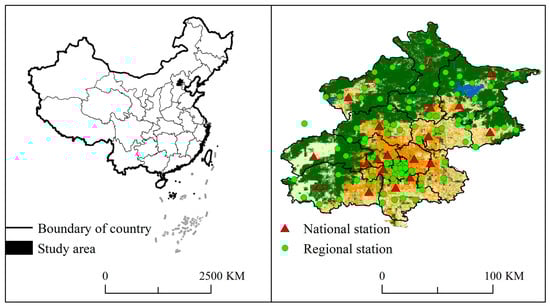
Figure 1.
Study area and meteorological station distribution.
2.2. Analysis Framework for the Spatiotemporal Distribution Characteristics of SDHR Based on the K-Shape Clustering Algorithm
The technical framework for the analysis is shown in Figure 2, which can be divided into three main steps.

Figure 2.
Framework for analyzing the spatiotemporal distribution characteristics of SDHR based on the K-shape clustering algorithm.
Step 1: Given the burstiness and localized nature of SDHR events, rainfall samples are selected based on both rainfall intensity and the spatial extent of the rainfall area, using hourly data from meteorological observation stations. By digitally encoding multiple SDHR events, a high-dimensional array is constructed that captures both the temporal and spatial distribution characteristics of the rainfall. This array enables a comprehensive digital representation of all the SDHR events.
Step 2: The high-dimensional array is then transformed into a fully connected form to construct a sequence of SDHR sample sequences. The K-shape clustering algorithm is then applied to iteratively optimize the class centers of the sample sequence set. The algorithm calculates the shape similarity between each sample and the corresponding class center to classify the SDHR events into different groups.
Step 3: Temporal and spatial distribution features of rainfall, such as the coefficient of variation of rainfall time, rainfall development duration, spatial variance coefficient, and spatial centroid of rainfall, are used to perform a comparative analysis of the spatiotemporal distribution characteristics of different types of SDHR events in Beijing.
2.2.1. Digital SDHR Process
- (1)
- Screening of SDHR samples
Currently, there is no unified definition of SDHR. The National Meteorological Center defines SDHR operationally as rainfall exceeding 20 mm/h. However, to identify SDHR events with significant spatiotemporal variations, we adopt the method used by the Beijing Meteorological Center, as outlined in Li Chen’s study [61]. This approach sets screening criteria based on both rainfall intensity and precipitation area. The proportion of stations and precipitation thresholds are determined through a comprehensive analysis of historical rainfall and disaster data in Beijing, ensuring a more accurate representation of SDHR dynamics in urban flood risk assessment.
The specific screening criteria are shown in Table 1. An SDHR event is considered to have occurred if any of the following three conditions are met. The screening process follows a reverse order, beginning with Condition 3. If Condition 3 is not satisfied, the sample is then assessed according to Condition 2. If Condition 2 is also not met, the sample is evaluated based on Condition 1. This sequential approach not only improves computational efficiency but also ensures the independence of each heavy rainfall sample. Using this method, a total of 105 SDHR events that met the screening criteria were identified for the period from 2009 to 2021.

Table 1.
Screening criteria for SDHR sample selection.
- (2)
- Digital processing of SDHR samples
The digitalization of SDHR samples aims to represent the spatiotemporal distribution of precipitation in a numerical format. Each rainfall event exhibits a unique data distribution pattern, and this approach enables the application of mathematical tools for further analysis.
For each SDHR sample, a high-dimensional array is constructed in both the temporal and spatial dimensions. Specifically, a rainfall event involves data from n time periods and s rain gauge stations. The digitalization process of the rainfall event consists of constructing a high-dimensional array that incorporates information from these time periods and stations. For a set of N SDHR samples, there will be N high-dimensional arrays. By using this method, a sample set of rainfall processes, denoted as , is established, which facilitates the digital representation of multiple rainfall events, as shown in the following equation:
Then, Qi is transformed into QTi for K-shape clustering analysis:
In this equation, represents the SDHR sample set, which includes N SDHR events. is the fully connected form of the i-th rainfall sample. The variables involved are as follows: is the rainfall amount at the s-th rain gauge station at the tn-th time, , , s is the number of rain gauge stations; n is the number of time periods.
2.2.2. Classification of SDHR Events Using the K-Shape Algorithm
The K-shape algorithm, proposed by Paparazzo et al. [62], is a time series clustering method based on shape similarity. K-shape is well suited for SDHR datasets analysis due to its (1) temporal phase alignment—using a normalized cross-correlation distance metric, it aligns time series by shape rather than timing, capturing phase shifts in rainfall peaks that traditional methods like K-means fail to address. (2) Amplitude normalization—it normalizes rainfall amplitudes, reducing biases from intensity differences (e.g., 50 mm/h vs. 30 mm/h) and focusing on structural similarities. (3) Computational efficiency—it balances accuracy and speed, outperforming computationally expensive DTW-based methods, making it scalable for high-resolution SDHR datasets (Table 2).
Table 2.
Comparison of clustering algorithms for SDHR datasets analysis.
K-shape is an iterative process that groups time series data by continuously optimizing cluster centers and reassigning members. Each iteration consists of two main steps.
Step 1: Cluster center extraction: The center for each cluster is computed based on the time series data within the cluster.
Step 2: Member assignment: Each time series is compared to all cluster centers, and based on shape similarity, it is assigned to the closest cluster center, thereby updating the cluster membership.
This iterative process continues until the cluster membership stabilizes or the maximum number of iterations is reached. The shape similarity measure and the cluster center extraction method are crucial in this process, as they directly impact the accuracy of the clustering results.
In this study, the K-shape algorithm is applied to the fully connected form of the constructed SDHR sample set φ, resulting in a classification of different types of SDHR events.
- (1)
- Shape similarity measurement method
To efficiently measure the shape similarity between time series, the K-shape algorithm uses cross-correlation as a similarity metric. Specifically, given two fully connected rainfall time series and , with Y remaining fixed, the time series X is shifted relative to y to compute the cross-correlation at various displacements. The relative displacement of the sequences is expressed as follows:
where indicates that sequence X has shifted s units to the right; and indicates that sequence X has shifted s units to the left. When , there will be 2m − 1 possible shift scenarios for the two time series. Then, the cross-correlation for each shift scenario is calculated to assess the degree of shape similarity between the two time series at different shifts.
The cross-correlation metric between X and Y is defined as follows: ; the calculation method for is as follows:
where is the local inner product calculation, representing the cross-correlation between sequence X and sequence Y at position w. Here, k refers to the relative offset between sequence X and sequence Y.
The purpose of this step is to identify the value of the parameter w that maximizes the cross-correlation between the time series X and Y. This parameter w represents the lag or shift where the similarity measure between X and Y is the highest. Once the optimal w is determined, we can calculate the corresponding shift of X relative to Y, denoted as x(s), where s is the difference between w and m: s = w − m.
To enhance computational efficiency and address the differences in time series data, the K-shape algorithm utilizes coefficient normalization, specifically the z-score method, to normalize the cross-correlation sequence. The definition of the normalized cross-correlation is as follows:
The normalized cross-correlation coefficient ranges from [−1, 1], where 1 means complete positive correlation and −1 means complete negative correlation. A Shape-Based Distance (SBD) of 0 signifies identical time series shapes, while a value of 2 indicates complete opposition. Once the centroid is determined, the SBD is used to assign time series to the nearest cluster based on shape similarity.
- (2)
- Cluster centroid extraction method
In time series clustering analysis, centroid extraction is a crucial step, as it directly determines the representative data point for each category. This representative data point, or cluster centroid, reflects the overall trend and characteristics of the time series data for that category.
The traditional method for extracting a class centroid involves calculating the arithmetic mean of the corresponding coordinates from all sequences in that category. However, this approach often fails to accurately capture the essential features of time series data. To overcome this limitation, the K-shape algorithm redefines centroid extraction as an optimization problem. For each class, the algorithm seeks to identify a center sequence () that maximizes the similarity, measured by the normalized cross-correlation (NCCc), with all time series in that class. The formula for this optimization is as follows:
In this formula, denotes the initial cluster center of the k-th class, while represents the complete dataset for that class. By integrating this with Equation (6), Equation (9) can be reformulated as follows:
Since all time series have been aligned to the reference sequence (the initial centroid ), the self-correlation term in the denominator can be disregarded. This omission is valid because, during the alignment process, each sequence has been shifted according to its maximum cross-correlation value with the centroid , thus optimizing . At this stage, the relative position between each sequence and the centroid is established, rendering the self-correlation term unnecessary for determining the centroid’s position. Vectorizing Equation (10) yields
To facilitate the solution, the optimization problem in Equation (8) is reformulated as a Rayleigh Quotient maximization problem. We introduce a matrix S, where the elements represent the inner products of all aligned time series. To center the matrix , we define a centralization matrix Q, such that and . Here, I denotes the identity matrix, and O is a matrix in which all elements are equal to 1. Furthermore, to ensure that has unit norm, Equation (11) is divided by . Finally, substituting S into results in
Ultimately, the centroid is determined by calculating the eigenvector associated with the maximum eigenvalue of the matrix M = QT·S·Q.
2.2.3. Analysis Method of Spatiotemporal Characteristics of SDHR
After applying the K-shape clustering method to classify SDHR events, this study uses indicators such as the coefficient of variation of rainfall, the frequency of occurrence of rainfall stations, rainfall growth time, and the spatial centroid of rainfall to perform a comparative analysis of the spatiotemporal distribution characteristics of different types of SDHR in Beijing. The following section provides a detailed introduction to the indicators that characterize the degree of spatiotemporal distribution unevenness, rainfall burstiness, and spatial heterogeneity.
- (1)
- The uneven spatiotemporal distribution of rainfall
This study uses the coefficient of variation of rainfall (Cv) to quantify the degree of spatiotemporal distribution unevenness of SDHR in Beijing from 2009 to 2021. The calculation formula for the coefficient of variation of rainfall is as follows:
where ; when calculating the temporal coefficient of variation, xi represents the precipitation amount at the i-th time period, is the average precipitation amount in the i-th time period, and n is the total number of hours of rainfall. When calculating the spatial coefficient of variation, xi represents the cumulative precipitation at the i-th rain gauge station, is the average cumulative precipitation across all stations, and n is the number of rain gauge stations. Based on the annual rainfall data for Beijing from 2009 to 2021, and considering the spatiotemporal distribution of rainfall in northern China, a critical value of Cv = 1.0 is selected to assess the uniformity of rainfall distribution. The coefficient of variation (Cv) threshold of 1.0 is adopted to classify rainfall uniformity, following regional studies of northern China’s convective systems [63]. This threshold statistically distinguishes homogeneous stratiform rainfall (Cv ≤ 1.0) from heterogeneous convective extremes (Cv > 1.0) based on their spatiotemporal variability characteristics [63]. When Cv ≤ 1.0, the rainfall is considered uniformly distributed in time or space; when Cv > 1.0, the distribution is considered uneven.
- (2)
- The burstiness of the rainfall
This study uses the growth time (GT) as an indicator to characterize the burstiness of rainfall. Growth time refers to the time required from the start of rainfall to the occurrence of the peak rainfall intensity. The specific expression is as follows:
where is the time at which the rainfall peak occurs; is the time when rainfall begins. It is required that the hourly rainfall begins at the start of rainfall. PREstart must be greater than 0.1 mm, and the hourly rainfall at the peak time, PREpeak, must be no less than 20 mm.
Since this study uses hourly rainfall observation data, the unit of GT is measured in hours. If, within an SDHR event, more than 50% of the stations that experience the event have a growth time of no more than 1 h, the event is considered to exhibit burstiness. Additionally, to characterize the spatial distribution of SDHR burstiness, this study separately calculates the growth time for each of the 110 meteorological stations across all SDHR events. This allows for the identification of regions in Beijing where the burstiness of SDHR is particularly significant.
- (3)
- Rainfall spatial heterogeneity characterization
This study uses the rainstorm center location as an indicator to compare the spatial heterogeneity of different types of SDHR events. The spatial centroid of rainfall is used to quantitatively represent the rainstorm center location in a single rainfall event. The centroid is a spatial feature, and the spatial centroid of rainfall refers to the weighted average position of the rainfall amount within a specific time period.
When describing the distribution of rainstorm centers for different SDHR events, this study defines the rainfall spatial centroid as the weighted average position of the rainfall amount at the time of maximum precipitation during an SDHR event. The more dispersed the spatial distribution of rainstorm center locations across different events of a particular type of SDHR, and the wider the distribution range, the stronger the spatial heterogeneity of the rainfall, and the higher the forecasting difficulty. The calculation formula for the rainfall spatial centroid is as follows:
In the formula, xc and yc represent the coordinates of the centroid, xc and yc are the coordinates of the meteorological stations, and pi is the precipitation at the corresponding meteorological station during a specific time period.
3. Results
3.1. Spatiotemporal Clustering Results of SDHR in Beijing
In this study, we applied the K-shape clustering algorithm to classify 105 SDHR events in Beijing from 2009 to 2021, with the aim of identifying event groups exhibiting similar spatiotemporal distribution patterns. The clustering analysis revealed three distinct categories: the first category (Cluster 1) had the fewest samples, with 14 events, accounting for 13.3% of the total; the second category (Cluster 2) had the largest number of samples, with 50 events, comprising 47.6% of the total; and the third category (Cluster 3) contained 41 events, accounting for 39.1% of the total samples.
To further validate our clustering results, we compared them with the classification results of Sun Jisong et al. [49], which are widely recognized. Sun et al. classified extreme SDHR events in the Beijing area from 2006 to 2013 based on mesoscale circulation system (MCS) characteristics. They divided the events into two main categories: the first category consists of SDHR events caused by the merging or repeated development and decay of long-lived convective systems, while the second category includes events formed by multiple strong convective systems passing through convective rainbands, resulting in a train-effect type of rainfall. Furthermore, they subdivided the first category into two subtypes, mixed convective and deep convective, based on the relative position of the convective rainband’s centroid to the 0 °C height level. Events with the centroid above the 0 °C height level were categorized as deep convective SDHR.
During the overlapping period from 2009 to 2013, our clustering results showed significant consistency with the classification outcomes of Sun Jisong et al. [49] (as shown in Table 3). This not only provides preliminary validation for our clustering results but also demonstrates that the K-shape algorithm can effectively capture the spatiotemporal distribution characteristics of SDHR events. This finding supports our hypothesis that there may be distinct differences in the spatiotemporal distribution characteristics of different types of SDHR events in the Beijing area, which could be related to mesoscale circulation patterns or moisture characteristics. Such consistency not only validates the effectiveness of the K-shape clustering algorithm in classifying SDHR events but also establishes a solid foundation for further analysis of the spatiotemporal distribution characteristics of various types of SDHR events.
Table 3.
Comparison of classification results for SDHR events in Beijing based on MCS characteristics and K-shape clustering algorithm.
3.2. Evaluation of the Spatiotemporal Distribution Unevenness of Rainfall for the Three Types of SDHR Events
Based on the K-shape clustering results, this study analyzed the spatiotemporal distribution unevenness of rainfall for SDHR events in Beijing. The box plot (Figure 3) shows that more than 96% of SDHR events have a temporal coefficient of variation greater than 1, and more than 88% of events have a spatial coefficient of variation greater than 1. This indicates that the rainfall in Beijing’s SDHR events exhibits significant heterogeneity in both its temporal and spatial distribution.
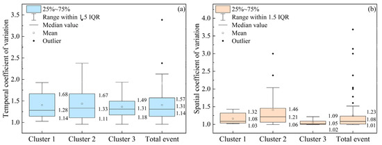
Figure 3.
Box plot statistics for the temporal coefficient of variation (a) and spatial coefficient of variation (b) of the three types of SDHR events (where Cluster 1 represents the first type of rainfall, Cluster 2 represents the second type, Cluster 3 represents the third type, and Total event represents all identified SDHR events; similar terminology applies to subsequent references).
In the temporal dimension, Cluster 2 exhibits the highest median temporal coefficient of variation (1.33), signifying the most pronounced unevenness in temporal distribution. Its box plot has the largest area and the widest data spread, suggesting that these events are more prone to experiencing intense rainfall over a short period. Cluster 3, with a median temporal coefficient of variation of 1.31, has the smallest box plot area and the most concentrated data, indicating a relatively uniform temporal distribution. Cluster 1 has a median temporal coefficient of variation of 1.28 and moderately concentrated data, implying that its temporal distribution is less uniform than that of Cluster 3 but not as uneven as that of Cluster 2. Overall, the degree of unevenness in the temporal distribution of rainfall follows the following order: Cluster 2 > Cluster 1 > Cluster 3.
In the spatial dimension, Cluster 2 again has the highest median spatial coefficient of variation (1.21), with a wide data distribution and a positive skew, indicating an extremely uneven spatial distribution of rainfall. Cluster 3 has a median spatial coefficient of variation of 1.05, located at the lower edge of the box, with highly concentrated data and little skew, showing a more uniform spatial distribution. Cluster 1 has a median spatial coefficient of variation of 1.08, also located at the lower edge of the box, with relatively concentrated data and little skew, indicating its spatial distribution unevenness is similar to that of Cluster 3, though slightly higher. The unevenness of rainfall’s spatial distribution follows the following order: Cluster 2 > Cluster 1 > Cluster 3.
The scatter plot (Figure 4) further reveals the spatiotemporal distribution characteristics of the three types of SDHR events. The points for Cluster 2 are widely distributed in the scatter plot, particularly in areas with a high coefficient of variation, which further emphasizes its significant unevenness in spatiotemporal distribution. The points for Cluster 3 are predominantly concentrated in areas with a low coefficient of variation, indicating a more uniform spatiotemporal distribution. The points for Cluster 1 are distributed in areas with a moderate coefficient of variation, showing a moderate level of unevenness in spatiotemporal distribution. The outliers in the scatter plot likely represent extreme rainfall events, with these being particularly more pronounced in Cluster 2.
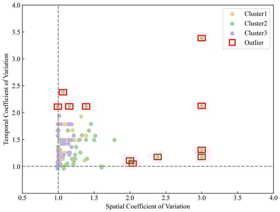
Figure 4.
Scatter plot distribution of the spatiotemporal coefficient of variation for the three types of SDHR events.
The scatter plot (Figure 4) further reveals the spatiotemporal distribution characteristics of the three types of SDHR events. The x-axis represents the spatial coefficient of variation, and the y-axis represents the temporal coefficient of variation, providing clarity on their respective meanings. The points for Cluster 2 are widely distributed, particularly in areas with a high coefficient of variation, which further emphasizes its significant unevenness in spatiotemporal distribution. The points for Cluster 3 are predominantly concentrated in areas with a low coefficient of variation, indicating a more uniform spatiotemporal distribution. The points for Cluster 1 are distributed in areas with a moderate coefficient of variation, showing a moderate level of unevenness in spatiotemporal distribution. Outliers, highlighted explicitly by red boxes (Cv ≥ 2), represent extreme rainfall events and are notably more pronounced in Cluster 2.
The advantage of the rainfall coefficient of variation is its ability to directly and simply describe the unevenness of SDHR in both temporal and spatial dimensions. However, it does not provide in-depth insights into the specific timing characteristics, spatial distribution patterns, or interactions with other meteorological factors of SDHR. To comprehensively compare the spatiotemporal distribution characteristics of the three types of SDHR events, we further analyzed the diurnal and monthly variation characteristics of their occurrence frequency. This helps to reveal the diurnal and seasonal patterns of SDHR. Additionally, we examined the suddenness characteristics of these events, which aids in assessing the forecasting difficulty and potential impacts on urban drainage systems.
In terms of spatial distribution characteristics, we conducted an in-depth analysis of the high-frequency areas and localized features of SDHR, which is crucial for identifying regions vulnerable to such events and providing a foundation for urban planning and flood control measures. Moreover, we analyzed the location of the rainstorm center and the movement of rainfall bands, which enhances the understanding of the dynamic changes in SDHR systems and provides a scientific basis for the development of precipitation forecasting and early warning systems.
3.3. Temporal Distribution Characteristics of the Three Types of SDHR
3.3.1. Daily and Monthly Variation Characteristics
Figure 5a–c illustrate the diurnal variation characteristics of station frequencies for the three types of SDHR events in Beijing from 2009 to 2021. Cluster 1 exhibits a multi-peak diurnal pattern, with the most active period occurring around noon, although the peak values lack distinct characteristics. Cluster 2 displays a bimodal diurnal variation, with the most active period between 8 AM and 12 PM, with peaks typically occurring around noon and in the afternoon. Cluster 3, on the other hand, shows a single-peak diurnal variation, with the most active period between 2 PM and 8 PM, with the peak usually occurring around 3 PM.

Figure 5.
Diurnal variation (a–c) and monthly variation (d) of SDHR frequencies at 110 rainfall stations in Beijing from 2009 to 2021.
By combining the daily and monthly variation characteristics, it was found that these features might be related to the formation conditions of different types of SDHR. Cluster 1 tends to occur around midday in early summer, which aligns with the formation conditions of mixed convective SDHR. This type of rainfall may be influenced by different weather systems at various times of the day, especially during early summer when weather systems are highly variable, facilitating the occurrence of mixed convective rainfall. Cluster 2 tends to occur in August around midday or in the afternoon, which corresponds with the formation conditions of deep convective SDHR. During the peak of summer, high temperatures and humidity—especially in the midday to afternoon period—create a significant temperature difference between the surface and upper layers, leading to unstable stratification favorable for the development of strong convective weather. Cluster 3 tends to occur in the afternoon to evening in July, which may be related to the formation conditions of train-effect SDHR. This type of rainfall typically occurs under specific summer weather systems, such as the post-cold vortex weather systems from the northeast, which bring the convergence of cold and warm air in the afternoon to evening, triggering rainfall.
3.3.2. Statistical Analysis of Key Rainfall Characteristics
The box plots presented in Figure 6 reveal significant differences across the three types of SDHR events in four key rainfall characteristics. Cluster 1 exhibits relatively low values for rainfall duration, daily accumulated precipitation, and average daily accumulated precipitation, with a concentrated data distribution. Although Cluster 2 shows lower median values for rainfall duration and daily accumulated precipitation compared to Cluster 3, its range of variation is notably wider, indicating greater data dispersion. Furthermore, both the maximum hourly precipitation and daily accumulated precipitation display a positive skew. Cluster 3, on the other hand, has the longest average rainfall duration, with overall higher daily precipitation amounts. The mean of the daily accumulated precipitation is the highest, and its distribution is more symmetric, suggesting that the daily accumulated precipitation in this cluster is generally larger.

Figure 6.
Box plot statistics for rainfall duration, maximum hourly precipitation, daily accumulated precipitation, and average daily precipitation for the three types of SDHR events and all SDHR events: (a) rainfall duration, (b) maximum hourly rainfall, (c) daily accumulated precipitation, and (d) average daily precipitation.
To statistically validate the observed inter-cluster differences, we performed the Kruskal–Wallis H test on four key precipitation indices (Table 4 and Table 5). The results show that, at the 95% confidence level, maximum hourly precipitation (H = 7.27, p = 0.026), rainfall duration (H = 13.97, p < 0.001), and average daily accumulated precipitation (H = 28.28, p < 0.001) have significant differences between clusters. Notably, average daily accumulated precipitation shows the strongest statistical separation (H = 28.28), confirming distinct precipitation intensity characteristics between clusters. However, daily accumulated precipitation shows no significant difference (H = 1.48, p = 0.476). These statistical validations confirm that the three-cluster classification effectively captures significantly different precipitation regimes in terms of temporal distribution and intensity characteristics.
Table 4.
Statistical table of key rainfall characteristics.
Table 5.
Statistical testing of key rainfall characteristics.
From the statistical analysis of these key rainfall characteristics, it can be concluded that Cluster 1 exhibits relatively low values across all key indicators, suggesting that these events tend to have lower intensity and shorter duration. Cluster 2 shows a large variability in maximum hourly rainfall intensity and daily accumulated precipitation, with a right-skewed distribution, which may indicate that these events are capable of producing extreme rainfall in certain cases. Cluster 3 is characterized by longer rainfall duration and higher daily accumulated precipitation, suggesting that these events are more significant in terms of both duration and total rainfall accumulation.
Drawing from the mesoscale systems and moisture characteristics associated with the three types of SDHR events, it can be inferred that Cluster 1 rainfall events are likely related to convective activities in lower temperature layers during mixed convection-type rainfall processes. These activities limit the intensity and duration of the precipitation, resulting in relatively small rainfall amounts and shorter durations. Cluster 2 events are likely associated with deep convection-type rainfall, driven by intense mesoscale convective systems that provide abundant moisture and unstable energy, leading to strong upward motion and precipitation and, consequently, extreme rainfall within a short period. Cluster 3 events may be linked to train-effect-type rainfall, where stable mesoscale circulation and sustained moisture supply cause cumulative effects in both time and space, leading to increased daily accumulated rainfall.
3.3.3. Analysis of Burstiness Characteristics
In the analysis of 105 SDHR events in Beijing, we found that over 66.9% of the rainfall stations reached maximum rainfall intensity within 1 h from the onset of precipitation, which significantly reflects the sudden nature of SDHR events in Beijing (Figure 7). Specifically, both Cluster 2 and Cluster 3 exhibit strong burstiness, with approximately 72.5% and 70.7% of the stations reaching their peak rainfall within 0–1 h, respectively. Although there is a slight increase in the percentage of stations reaching peak rainfall during the 5–8 h period, the likelihood of these two types of SDHR events reaching peak intensity significantly decreases as time progresses. In contrast, Cluster 1 shows less burstiness, with only about 44.3% of the stations reaching peak intensity within 0–1 h. Additionally, for the 2–4 h, 5–8 h, and 9–12 h periods, approximately 16.1%, 16.1%, and 20% of the stations in Cluster 1 reached peak intensity, indicating that the peak rainfall times in Cluster 1 are more spread out.
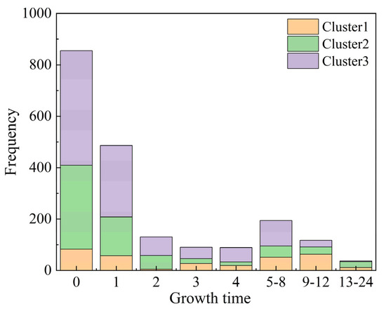
Figure 7.
Distribution of rainfall growth time at 110 automatic rain gauge stations in Beijing during three types of SDHR events.
Figure 8 illustrates the overall spatial distribution of burstiness in SDHR events in Beijing, while Figure 9 presents the spatial distribution of burstiness characteristics for the three types of SDHR events in Beijing. Stations with a higher frequency of rainfall events developing in less than 1 h indicate stronger burstiness. Through visual inspection complemented by quantitative spatial clustering analysis using the Global Moran’s I statistic, significant clustering of burstiness was observed (Moran’s I = 0.357, p < 0.0001), particularly concentrated in the southwestern mountainous area, central urban area, and northeastern plain area, displaying an increasing trend from southwest to northeast. Cluster-specific analysis shows that Cluster 1 demonstrates moderate spatial clustering of low-intensity burstiness primarily in the southern region, with minimal presence elsewhere. Cluster 2 reveals statistically significant clustering of strong burstiness in the northeastern region. Meanwhile, Cluster 3 exhibits strong spatial clustering prominently within the central urban area and northeastern plain.
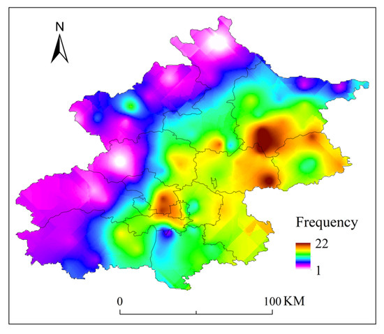
Figure 8.
Frequency distribution of stations reaching peak rainfall within 1 h during SDHR events at 110 automatic rain gauge stations in Beijing.
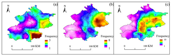
Figure 9.
Frequency distribution of stations reaching peak rainfall within 1 h during three types of SDHR events at 110 automatic rain gauge stations in Beijing: (a) cluster 1; (b) cluster 2; (c) cluster 3.
The burstiness of SDHR not only manifests as its abrupt onset but also in the high intensity of rainfall, which can lead to sudden flooding disasters in a region. Therefore, to further assess the vulnerability of areas facing SDHR, we analyzed the range of peak rainfall values for events with a development time of less than 1 h at each rain gauge station during the three types of SDHR events (as shown in Figure 10). We hypothesize that the larger the range of peak rainfall values for events with a development time of less than 1 h, the greater the vulnerability of that station to SDHR.
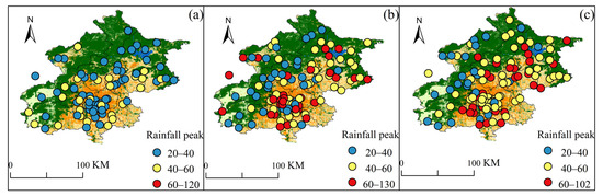
Figure 10.
Range of rainfall peak values (mm/h) for SDHR events with a growth time of less than 1 h at 110 automatic rain gauge stations in Beijing during three types of SDHR events: (a) cluster 1; (b) cluster 2; (c) cluster 3.
Comparative analysis of the subfigures in Figure 10 reveals that the vulnerability of stations in Cluster 3 to SDHR is significantly higher than that of Cluster 2 and Cluster 1. In the entire plain region, the rainfall peaks exceed 40 mm/h, with a maximum rainfall peak of 102 mm/h. Stations in Cluster 1 show relatively lower vulnerability, but at locations with strong suddenness, rainfall peak values exceed 40 mm/h, placing considerable pressure on local drainage systems. Although Cluster 2 stations are less vulnerable than Cluster 3, some stations with high suddenness, such as those in the central urban area, have rainfall peak values up to 130 mm/h, far exceeding the design standard for the city’s drainage network, which is based on a once-in-10-years event. This significantly increases the risk of flooding.
Therefore, in flood prevention and mitigation efforts, it is crucial to pay special attention to the time and spatial distribution characteristics of the suddenness of different types of SDHR. Targeted flood control and drainage measures should be implemented accordingly.
3.4. Spatial Distribution Characteristics of the Three Types of SDHR
3.4.1. High-Frequency Areas and Locality
After analyzing the frequency of SDHR events at each rain gauge station, we found that the regions in Beijing most frequently experiencing such events are concentrated in the southwestern mountainous areas, the central urban area, and the northeastern plains (as shown in Figure 11), with the northwestern mountainous area exhibiting the fewest occurrences. By comparing the spatial distribution of the maximum hourly rainfall intensity (as shown in Figure 12), it was observed that these three regions also coincide with areas where the average total rainfall is relatively high. The overlap between high-frequency and high-intensity zones may be closely related to the region’s topography and moisture conditions. In the southwestern mountainous areas, the topographic uplift effect causes southeast winds to be lifted by the western mountain terrain, forming orographic rainfall, which leads to concentrated precipitation. The urban heat island effect in the central urban area enhances atmospheric convection instability, promoting the development of convective clouds and intensifying precipitation. In the northeastern plains, the presence of the Miyun Reservoir provides ample moisture, and the influence of multiple moisture transport channels offers a rich source of water vapor for the storms.
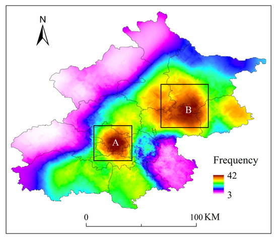
Figure 11.
Frequency distribution of SDHR events at 110 automatic rain gauge stations in Beijing.

Figure 12.
Distribution of average total rainfall volume at 110 automatic rain gauge stations in Beijing during SDHR events.
Further analysis of the high-frequency and high-intensity areas of the three types of SDHR events (as shown in Figure 13 and Figure 14) reveals a high degree of spatial overlap. However, significant differences exist in the specific locations and extents of these areas across different types of SDHR. For Cluster 1, the high-frequency and high-intensity areas are primarily distributed from the western foothills of Beijing to the southeastern regions, with the probability of Cluster 1-type heavy rainfall reaching up to 50% in these areas. In contrast, Cluster 2 shows different distributions, with the high-frequency areas concentrated in the central urban area and northeastern plains, while the high-intensity areas are primarily located in the northeastern plains, where the probability of Cluster 2-type heavy rainfall can reach as high as 72%. Cluster 3 has the widest distribution of high-frequency and high-intensity areas, mainly concentrated in the central urban area and northeastern plains, where the probability of Cluster 3-type heavy rainfall reaches up to 49%.
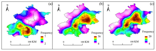
Figure 13.
Frequency distribution of occurrences at 110 automatic rain gauge stations in Beijing during three types of SDHR events: (a) cluster 1; (b) cluster 2; (c) cluster 3.

Figure 14.
Distribution of average total rainfall volume at 110 automatic rain gauge stations in Beijing during three types of SDHR events: (a) cluster 1; (b) cluster 2; (c) cluster 3.
By comparing the coverage of the high-frequency areas, this study further analyzes the localized characteristics of the three types of SDHR and suggests that the smaller the coverage of the high-frequency areas, the stronger the locality. Overall, there are significant differences in the coverage of the high-frequency areas for the three types of SDHR. Cluster 1 has the smallest high-frequency area, with the most pronounced localized characteristics; Cluster 3 has the largest high-frequency area, with relatively weaker locality; Cluster 2 falls in between, exhibiting some localized characteristics. In conjunction with the formation mechanisms of the three types of SDHR, it is speculated that this difference may be related to the water vapor transport and the organization of convective activity. Mixed convection-type rainfall is primarily formed by warm and humid air flows from the southeast, which are uplifted by terrain. Convective cells typically form and intensively develop in areas where low-level shear lines and surface convergence lines intersect, with rainfall mainly occurring in the lower troposphere. Therefore, Cluster 1 has a smaller rainfall area and stronger locality. Deep convection-type heavy rainfall is typically associated with intense vertical convective activity, with faster-moving air masses, resulting in a larger rainfall area for Cluster 2 compared to Cluster 1. Train-effect-type heavy rainfall is caused by the interaction of two convective rain bands with different thermal characteristics (cold and warm), leading to a wider distribution of rainfall in Cluster 3, with the least pronounced localized characteristics.
3.4.2. Characteristics of the Rainstorm Center Area
From the spatial distribution of the rainstorm center areas of different types of SDHR events (as shown in Figure 15), Cluster 1 has the smallest range of rainstorm centers, which are primarily concentrated in the foothill plain areas, although the location of the rainstorm center varies across different events. Cluster 2 has the largest range of rainstorm centers, widely distributed in the southwestern foothill plain areas, the central urban area, and extending to the northeastern plains, with an east–west orientation. The rainstorm center range of Cluster 3 is slightly smaller than that of Cluster 2, primarily distributed along a southwest–northeast diffusion belt. Therefore, based on the range of rainstorm center areas for the three types of SDHR events, the spatial heterogeneity of rainfall is ranked as follows: Cluster 2 > Cluster 3 > Cluster 1.
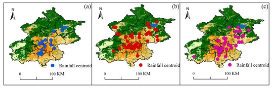
Figure 15.
Spatial distribution of rainstorm centers during the three types of SDHR in Beijing: (a) cluster 1; (b) cluster 2; (c) cluster 3.
In a given type of SDHR, the more frequently the rainstorm centers appear in the same location across different events, the higher the likelihood that this area will become the rainstorm center for that type of event. As shown in Figure 15, the aggregation areas of the rainstorm centers for the three types of SDHR events differ. The rainstorm centers of Cluster 1 are more dispersed, with the western foothill areas being more likely to become the rainstorm center for Cluster 1. For Cluster 2, the aggregation area of the rainstorm centers is primarily located in the central urban area and its surrounding regions, indicating that the central urban area is more likely to become the rainstorm center for Cluster 2. The rainstorm centers of Cluster 3 are mainly concentrated in the southwestern and central urban areas along the rainfall center diffusion belt, suggesting that these regions are more likely to become the rainstorm center for Cluster 3.
It is worth noting that the rainstorm centers in all three types of SDHR events tend to occur in areas with a high urbanization rate near the foothills. This phenomenon further confirms that the blocking and lifting effects of the foothill topography, as well as the convective instability caused by the urban heat island effect, may significantly amplify the convective processes of SDHR. Particularly in the southwestern foothills, where the central urban area has the highest level of urbanization, this area is more likely to become the rainstorm center in all three types of SDHR events. By combining Figure 9 and Figure 10, it can be observed that the central urban area is a region with a high degree of suddenness in SDHR, especially in Cluster 2, where extreme rainfall peaks are common, and Cluster 3, characterized by large total rainfall and long durations. Therefore, it is essential to pay special attention to flood control and drainage efforts in the central urban area.
3.4.3. Rainband Movement Characteristics
The spatial heterogeneity of rainfall is not only reflected in the magnitude and distribution of regional precipitation but also in the movement of the rainstorm center. In certain SDHR events, when some areas experience sustained and excessively intense rainfall, it is crucial to pay attention. Due to the complex weather systems that generate Cluster 1 and Cluster 2 events, the spatial distribution of rainbands at different times is relatively dispersed. Using rainstorm centers from different time points alone may not accurately reflect the overall movement of the rainband. Therefore, in this study, we selected a representative SDHR event from each of the three clusters to illustrate both the static distribution characteristics of the rainband at each time point and the dynamic movement characteristics of the rainband over time.
Figure 16, Figure 17 and Figure 18 show the spatial distribution of the rainband at each time point during three typical SDHR events. A comparison reveals that the three types of SDHR exhibit distinct characteristics in terms of both the static spatial distribution and the dynamic movement of the rainband. For Cluster 1, rainfall typically begins in the southeastern area of Beijing, gradually moving toward the urban area and the northern region, ultimately spreading in the northeastern direction (Figure 16). For Cluster 2, rainfall generally starts in the northwestern mountainous area of Beijing, gradually moving toward the urban area and the southern region, eventually spreading in the southern direction (Figure 17). For Cluster 3, rainfall usually starts in the southwestern area of Beijing, gradually moving toward the urban area and the northeastern region, eventually spreading in the northeastern direction (Figure 18).
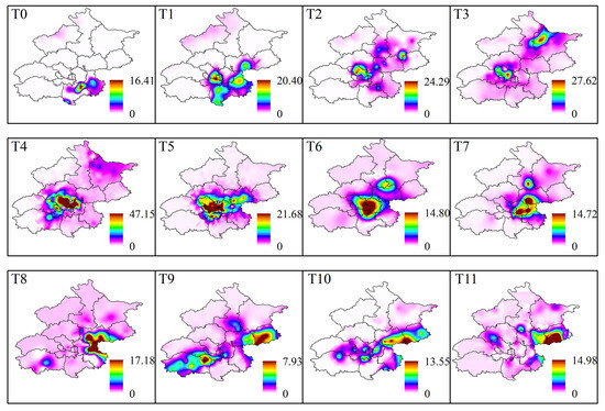
Figure 16.
Rainband movement characteristics of the typical heavy rainfall process in Cluster 1 of SDHR events.
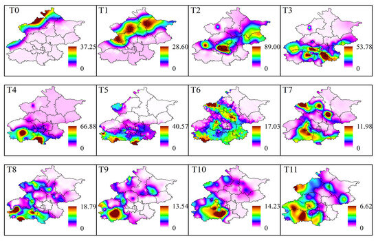
Figure 17.
Rainband movement characteristics of the typical heavy rainfall process in Cluster 2 of SDHR events.
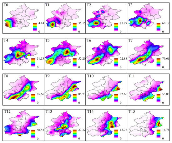
Figure 18.
Rainband movement characteristics of the typical heavy rainfall process in Cluster 3 of SDHR events.
Through comparative analysis, the movement of the rainband in the three types of SDHR events is likely related to the pathways of moisture transport and the development of convective activity. For Cluster 1 and Cluster 2, the moisture primarily comes from the southeast low- and middle-level airflows. The orographic lifting on the windward slope easily triggers the release of convective instability energy, and convective cells typically initiate and develop at the intersection of low-level shear lines and surface convergence zones, subsequently moving along the direction of the southeast airflow. The rainfall process in Cluster 1 is typically associated with the warm cloud process, with precipitation mainly occurring in the lower layers of the troposphere, resulting in smaller rainfall amounts and more limited spatial coverage. In contrast, the rainfall process in Cluster 2 is mainly dominated by cold cloud processes, driven by strong convective activity. The convective cells experience greater vertical lift, and the air mass as a whole moves southeastward more rapidly, leading to higher rainfall amounts and a broader coverage area. For Cluster 3, the moisture primarily originates from two branches of warm and moist monsoon flows from the Bay of Bengal and the western Pacific. The movement vectors of the convective cells are nearly parallel to the distribution of the rainband, and the precipitation distribution typically follows the axis of low-level jet streams, resulting in the broadest rainband coverage. Due to the sequential passage of multiple convective cells over the same area, the duration of rainfall and the cumulative precipitation are generally higher.
4. Discussion
4.1. Reliability of the K-Shape Algorithm in Identifying SDHR Events with Similar Spatiotemporal Patterns
4.1.1. Comparative Verification of the K-Shape Algorithm for SDHR Classification
To assess the reliability of the K-shape algorithm in identifying SDHR events with similar spatiotemporal patterns, comparative experiments were conducted using K-means and DTW clustering algorithms under the same K value. As shown in Table 6, the optimal number of clusters for K-means, DTW, and K-shape were 2, 3, and 3, respectively, leading to the selection of K = 3 for further comparison. The silhouette coefficients for K = 3 were 0.425 for K-means, 0.442 for DTW, and 0.254 for K-shape, which may initially suggest that K-shape’s clustering effectiveness is lower than that of K-means and DTW. However, to comprehensively evaluate its performance, a deeper analysis was conducted based on temporal and spatial similarity. Temporal similarity was assessed by analyzing the hourly distribution of rainfall within each identified sample group, while spatial similarity was evaluated by comparing rainfall distributions across different sites.
Table 6.
Optimal cluster numbers and silhouette coefficients for K-means, DTW, and K-shape algorithms.
Figure 19, Figure 20, Figure 21, Figure 22, Figure 23 and Figure 24 illustrate the spatial and temporal rainfall distributions of the most similar sample groups identified by each algorithm. The K-means results (Figure 19 and Figure 20) show dissimilar spatial rainfall distributions but relatively similar temporal patterns, indicating that K-means is more effective at capturing single-dimensional features rather than comprehensive spatiotemporal relationships. In contrast, the DTW results (Figure 20 and Figure 21) reveal dissimilar and nearly opposite spatial and temporal distributions, likely due to DTW’s overcompensation in phase alignment, which reduces clustering reliability. Meanwhile, the K-shape results (Figure 22 and Figure 23) exhibit the highest degree of similarity in both spatial and temporal distributions, demonstrating its superior ability to effectively capture spatiotemporal sequence data.
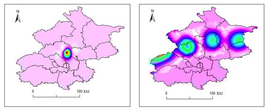
Figure 19.
Spatial distribution of rainfall in the most similar sample group identified by K-means (20150826, (left); 20150930, (right)).
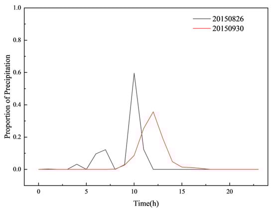
Figure 20.
Temporal distribution of rainfall in the most similar sample group identified by K-means.

Figure 21.
Spatial distribution of rainfall in the most similar sample group identified by DTW (20160827, (left); 20210913, (right)).

Figure 22.
Temporal distribution of rainfall in the most similar sample group identified by DTW.
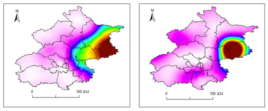
Figure 23.
Spatial distribution of rainfall in the most similar sample group identified by K-shape (20110706, (left); 20130806, (right)).
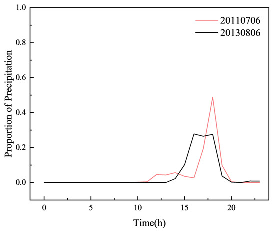
Figure 24.
Temporal distribution of rainfall in the most similar sample group identified by K-shape.
These results highlight the necessity of a dual evaluation method combining “indicator verification” (quantitative metrics such as silhouette coefficients) and “domain knowledge” (physical reasonableness of spatiotemporal distributions). While silhouette coefficients provide an initial assessment, they do not fully capture clustering effectiveness in real-world meteorological applications. The performance of the K-shape algorithm in SDHR classification suggests that specialized time series clustering techniques may offer superior applicability compared to general clustering methods. This finding underscores the importance of integrating spatiotemporal consistency in evaluating clustering effectiveness, providing a valuable technical approach for meteorological data mining.
4.1.2. Advancing SDHR Classification Through Multivariate Clustering
In this study, the K-shape clustering algorithm was applied to classify 105 SDHR events in Beijing (2009–2021), effectively identifying groups with similar spatiotemporal distribution patterns. The clustering results revealed three distinct categories, showing strong consistency with the classification of extreme SDHR events (2006–2013) based on mesoscale circulation characteristics [49]. This provides preliminary validation of the clustering results and highlights the high reliability of the K-shape algorithm in handling spatiotemporal two-dimensional structures in SDHR data.
The K-shape algorithm classifies SDHR events by capturing the shape features of time series data, iteratively optimizing class centers, and calculating shape similarity within each group. Its minimal data requirements—relying only on high spatiotemporal resolution precipitation data—make it a flexible and practical choice for real-world meteorological applications.
However, due to the complexity of meteorological systems, SDHR events are influenced by multiple dynamic factors beyond precipitation alone. Parameters such as the vertical structure of humidity, temperature gradient evolution, and wind field dynamics significantly affect convection triggering and moisture transport efficiency. The limitations of univariate clustering may lead to events with distinct physical mechanisms being grouped together based solely on precipitation characteristics, reducing classification accuracy in extreme weather attribution.
To overcome these limitations, multivariate clustering techniques should be introduced. Expanding the feature space to incorporate water vapor, thermal, and dynamic parameters would enhance the algorithm’s ability to capture interactions between key meteorological variables. This requires integrating high-resolution reanalysis data with multi-source observations, ensuring more comprehensive representation of SDHR processes. Additionally, local influences, such as urban canopy effects, may introduce spatial heterogeneity in near-surface meteorological elements, necessitating clustering models capable of spatial heterogeneity analysis for improved classification accuracy.
4.2. Summary of the Spatiotemporal Distribution Characteristics of the Three Types of SDHR
Cluster 1 exhibits a certain degree of spatiotemporal unevenness in its rainfall distribution. In terms of time, its daily variation follows a multi-peak pattern, with active periods concentrated around midday. The monthly variation is most frequent in early summer, particularly in June and July. Key rainfall characteristics indicate that the intensity and duration of this type of rainfall are relatively small, with no significant burstiness, and the timing of peak rainfall is more scattered. In terms of spatial distribution, high-frequency areas are concentrated in the western foothill urban areas and the southeastern region. The rainfall exhibits a strong localized character, with a small and dispersed area for the rainstorm centers. The rainbands generally move from the southeast toward the urban area and the northern part of the city, eventually spreading toward the northeast. Overall, this type of rainfall is characterized by weak burstiness and spatial heterogeneity, but it is more localized.
Cluster 2 exhibits a higher degree of spatiotemporal unevenness. In terms of time, the daily variation is bimodal, with the primary active periods in the morning and afternoon, occurring especially frequently in August during the peak of summer. Key rainfall characteristics show large variations in both rainfall duration and daily accumulated precipitation, with skewness toward higher values in the maximum hourly precipitation and daily accumulated precipitation. This type of rainfall has strong burstiness, with most stations reaching their peak within 1 h. Spatially, high-frequency and high-intensity areas are concentrated in the central urban area and the northeastern plain region. The rainstorm center area is widespread, extending in an east–west direction. Rainbands typically move from the northwest mountainous areas toward the urban area and the south, eventually spreading toward the southern regions. This type of rainfall is characterized by strong burstiness, weaker locality, and significant spatial heterogeneity. It is prone to causing extreme precipitation events in the central urban area, which can significantly impact urban operations.
Cluster 3 exhibits a low level of spatiotemporal unevenness. In terms of time distribution, it shows a unimodal daily variation, with the most active periods in the afternoon and evening. Monthly variation is higher in July and August. Key rainfall characteristics include longer rainfall duration, higher daily accumulated precipitation, and strong burstiness, with a higher proportion of stations reaching peak rainfall within 1 h. Spatially, the high-frequency and high-intensity areas cover the central urban area and the northeastern plain region, with the rainstorm center area slightly smaller than that of Cluster 2, following a southwest–northeast distribution. Rainbands move from the southwest toward the urban area and the northeast, eventually spreading in the northeastern region. This type of rainfall has weaker burstiness and locality but stronger spatial heterogeneity. Prolonged heavy rainfall exerts sustained pressure on urban flood control and drainage systems.
4.3. Vulnerability, Forecasting Difficulty, and Impact on Urban Flood Control and Drainage in Beijing in Response to Three Types of SDHR
Beijing exhibits varying degrees of vulnerability to the three types of SDHR events. Although Cluster 1 has lower intensity, its burstiness in the southern region can still strain local drainage systems. Cluster 2, with its high intensity, strong burstiness, and concentration in the central urban area, poses the greatest flood risk, particularly in densely populated zones with extensive infrastructure, leading to severe disruptions such as traffic paralysis and daily life disturbances. Cluster 3, characterized by prolonged rainfall and substantial accumulation, places sustained pressure on the drainage system in the central urban and northeastern plain regions, increasing the likelihood of prolonged waterlogging and operational strain on flood control infrastructure.
Table 7 presents statistical data on flood disasters triggered by SDHR events in Beijing from 2009 to 2013, categorized by rainfall clusters. The results highlight substantial variations in flood severity. Cluster 3 resulted in the most significant economic losses and highest affected populations, with the 21 July 2012 event (over 460 mm in 18 h) causing 79 fatalities and RMB 15.98 billion in damages [64]. Cluster 2, with its high-intensity rainfall concentrated in the central urban area, frequently led to severe flooding and traffic disruptions. Urbanization has exacerbated this issue, intensifying average rainfall within Beijing’s Sixth Ring Road by approximately 23% and increasing peak hourly intensities to 27 mm/h [65]. Although Cluster 1 events were less intense overall, localized high-burstiness episodes still challenged regional drainage systems. These findings emphasize the need for targeted drainage improvements and the incorporation of cluster-specific rainfall characteristics into flood risk assessments.
Table 7.
The situation of flood disasters caused by heavy rain in the Beijing area from 2009 to 2014.
Each SDHR type presents distinct forecasting challenges. Cluster 1 lacks significant burstiness, with scattered peak rainfall times, which increases the difficulty in predicting the exact occurrence time and intensity of the rainfall. Cluster 2 is characterized by large variations in rainfall intensity, strong burstiness, and the involvement of complex mesoscale convective systems and interactions with weather systems. This leads to substantial uncertainty in forecasting extreme rainfall amounts. Cluster 3, while benefiting from stable mesoscale circulation and ample moisture supply, poses challenges in accurately forecasting the total precipitation due to the prolonged rainfall process and cumulative effects. Additionally, differences in the storm center location and the movement path of the rainbands complicate the precise prediction of rainfall areas.
The differing impacts of SDHR types necessitate tailored flood control strategies. Cluster 1 primarily affects the southern region, requiring attention to localized drainage issues. Cluster 2 poses the greatest threat to the central urban area, where sudden heavy rainfall can easily lead to urban flooding, impacting transportation and residents’ daily lives. Strengthening drainage system construction and emergency response capabilities in the central urban area is essential. Cluster 3, with its prolonged heavy rainfall, continuously pressures the city’s drainage system, potentially causing long-term waterlogging in some areas. To mitigate the impact on the city’s economy and social activities, the overall response capacity and long-term operational stability of the city’s flood control and drainage system need to be improved.
5. Conclusions
This study applied the K-shape clustering algorithm to high-resolution hourly rainfall data from 105 stations in Beijing (2009–2021) to classify SDHR events and analyze their spatiotemporal patterns in relation to mesoscale circulation features. The findings provide valuable insights for urban flood management by identifying distinct rainfall types and their associated risks.
The results revealed three rainfall clusters with unique characteristics. Cluster 1, with moderate variability and minor intensity, is more prevalent in early summer and primarily affects the western mountainous to southeastern areas. Cluster 2, characterized by high variability and intense rainfall, predominantly impacts the urban core and northeastern plains, posing significant challenges due to its strong temporal burstiness and spatial heterogeneity. Cluster 3, exhibiting low variability but prolonged rainfall duration, places sustained pressure on flood control systems, particularly in the urban and northeastern plains, peaking in summer afternoons and evenings. These findings highlight Beijing’s differential vulnerability to various SDHR types, forecasting challenges, and the need for targeted flood management strategies.
A key innovation of this study is the application of the K-shape algorithm to SDHR classification, providing a novel approach to understanding spatiotemporal rainfall patterns. However, certain limitations must be acknowledged. First, spatial correlation analysis between rainfall intensity and urbanization levels was not explicitly conducted. Future research will integrate topographic, land use, and infrastructure data to assess how urbanization affects rainfall distribution. This will be achieved by inputting SDHR datasets into a physically based urban hydrodynamic model for a more comprehensive spatial analysis.
Second, potential uncertainties in the clustering process and data limitations should be considered. While the study benefits from 105 rain gauges covering Beijing’s main administrative areas, the lower station density in southeastern mountainous regions may underrepresent localized heavy rainfall features. Additionally, the current one-hour temporal resolution provides a general view of rainfall processes but may overlook finer-scale variations in storm center movement and intensity changes. To improve accuracy, future studies should incorporate higher temporal resolution data (e.g., 15 min or 5 min intervals) to better distinguish local vs. systematic rainfall patterns and enhance flood control planning.
Overall, this study underscores the importance of considering spatiotemporal heterogeneity in urban flood risk management and infrastructure planning. Addressing the identified limitations will refine the classification accuracy of SDHR events and improve forecasting and flood mitigation strategies in highly urbanized environments.
Author Contributions
Conceptualization, Z.Q. and Q.C.; methodology, Q.C.; software, Z.Q. and X.X.; validation, B.W. and S.J.; investigation, X.X.; resources, R.S.; data curation, Q.C. and S.J.; writing—original draft preparation, Z.Q. and S.J.; writing—review and editing, Q.C. and B.W.; visualization, Z.Q.; supervision, Q.C.; funding acquisition, Q.C. and B.W. All authors have read and agreed to the published version of the manuscript.
Funding
This research was funded by the National Basic Research Program of China (2023YFC3010704) and the Chinese National Natural Science Foundation (No. 52209004).
Data Availability Statement
The original contributions presented in this study are included in the article. Further inquiries can be directed to the corresponding author.
Acknowledgments
The authors sincerely thank the National Meteorological Data Center for providing essential data support and the National Natural Science Foundation of China for funding this research. We also extend our gratitude to the two anonymous reviewers for their insightful comments and constructive suggestions, which have greatly improved this paper.
Conflicts of Interest
The authors declare no conflicts of interest.
References
- Ayat, H.; Evans, J.P.; Sherwood, S.C.; Soderholm, J. Intensification of subhourly heavy rainfall. Science 2022, 378, 655–659. [Google Scholar] [CrossRef] [PubMed]
- Fowler, H.J.; Lenderink, G.; Prein, A.F.; Westra, S.; Allan, R.P.; Ban, N.; Barbero, R.; Berg, P.; Blenkinsop, S.; Do, H.X.; et al. Anthropogenic intensification of short-duration rainfall extremes. Nat. Rev. Earth Environ. 2021, 2, 107–122. [Google Scholar] [CrossRef]
- Chen, H.; Sun, J.; Chen, X.; Zhou, W. CGCM projections of heavy rainfall events in China. Int. J. Climatol. 2012, 32, 441–450. [Google Scholar] [CrossRef]
- Chen, P.-Y.; Tung, C.-P.; Tsao, J.-H.; Chen, C.-J. Assessing Future Rainfall Intensity–Duration–Frequency Characteristics across Taiwan Using the k-Nearest Neighbor Method. Water 2021, 13, 1521. [Google Scholar] [CrossRef]
- Li, H.; Cui, X.; Zhang, D.-L. A statistical analysis of hourly heavy rainfall events over the Beijing metropolitan region during the warm seasons of 2007–2014. Int. J. Climatol. 2017, 37, 4027–4042. [Google Scholar] [CrossRef]
- Myhre, G.; Alterskjær, K.; Stjern, C.W.; Hodnebrog, Ø.; Marelle, L.; Samset, B.H.; Sillmann, J.; Schaller, N.; Fischer, E.; Schulz, M.; et al. Frequency of extreme precipitation increases extensively with event rareness under global warming. Sci. Rep. 2019, 9, 16063. [Google Scholar] [CrossRef] [PubMed]
- Huang, J.; Cao, W.; Wang, H.; Wang, Z. Affect Path to Flood Protective Coping Behaviors Using SEM Based on a Survey in Shenzhen, China. Int. J. Environ. Res. Public Health 2020, 17, 940. [Google Scholar] [CrossRef]
- Lei, T.; Wang, J.; Li, X.; Wang, W.; Shao, C.; Liu, B. Flood Disaster Monitoring and Emergency Assessment Based on Multi-Source Remote Sensing Observations. Water 2022, 14, 2207. [Google Scholar] [CrossRef]
- Shan, Z.; Duan, W.; Christidis, N.; Jian-Li, D.; Nover, D.; Jilili, A.; De Maeyer, P.; Van de Voorde, T. An extreme rainfall event in summer 2018 of Hami city in eastern Xinjiang, China. Adv. Clim. Change Res. 2021, 12, 795–803. [Google Scholar]
- Chen, G.; Hou, J.; Hu, Y.; Wang, T.; Yang, S.; Gao, X. Simulated Investigation on the Impact of Spatial–temporal Variability of Rainstorms on Flash Flood Discharge Process in Small Watershed. Water Resour. Manag. 2023, 37, 995–1011. [Google Scholar] [CrossRef]
- Deng, P.; Zhang, M.; Hu, Q.; Wang, L.; Bing, J. Pattern of spatio-temporal variability of extreme precipitation and flood-waterlogging process in Hanjiang River basin. Atmos. Res. 2022, 276, 106258. [Google Scholar]
- Rafieeinasab, A.; Norouzi, A.; Kim, S.; Habibi, H.; Nazari, B.; Seo, D.-J.; Lee, H.; Cosgrove, B.; Cui, Z. Toward high-resolution flash flood prediction in large urban areas—Analysis of sensitivity to spatiotemporal resolution of rainfall input and hydrologic modeling. J. Hydrol. 2015, 531, 370–388. [Google Scholar]
- Deegala, D.; Song, Y.H.; Chung, E.-S.; Ayugi, B.O.; Shahid, S. Future extreme precipitation changes in the South Asian Summer Monsoon Dominance Region. Atmos. Res. 2023, 295, 107029. [Google Scholar]
- Lana, X.; Rodríguez-Solà, R.; Martínez, M.D.; Casas-Castillo, M.C.; Serra, C.; Burgueño, A. Characterization of standardized heavy rainfall profiles for Barcelona city: Clustering, rain amounts and intensity peaks. Theor. Appl. Climatol. 2020, 142, 255–268. [Google Scholar]
- Sojan, J.M.; Srivastav, R.; Meghana, N. Regional non-stationary future extreme rainfall under changing climate over Asian Monsoon Region. Atmos. Res. 2023, 284, 106592. [Google Scholar]
- Takhellambam, B.S.; Srivastava, P.; Lamba, J.; Zhao, W.; Kumar, H.; Tian, D.; Molinari, R. Artificial neural network-empowered projected future rainfall intensity-duration-frequency curves under changing climate. Atmos. Res. 2024, 297, 107122. [Google Scholar]
- Lei, N.; Gao, L.; Liu, S.; Zhou, Z. The Spatiotemporal Clustering of Short-Duration Rainstorms in Shanghai City Using a Sub-Hourly Gauge Network. Earth Space Sci. 2024, 11, e2023EA003442. [Google Scholar]
- Diaz, H.F.; Giambelluca, T.W. Changes in atmospheric circulation patterns associated with high and low rainfall regimes in the Hawaiian Islands region on multiple time scales. Glob. Planet. Change 2012, 98–99, 97–108. [Google Scholar]
- Xu, T.; Yang, Z.; Gao, X.; Zhou, J. A Study on the Evolution of Urban Underlying Surfaces and Extreme Rainfall in the Pearl River Delta. Water 2024, 16, 267. [Google Scholar] [CrossRef]
- Xing, N.; Zhang, Y.; Li, S.; Dai, Y.; Hao, C.; Li, J.; Zhi, X. The features and probability forecasting of short–duration heavy rainfall in the Beijing-Tianjin-Hebei region caused by North China cold vortices. Front. Environ. Sci. 2023, 10, 1101602. [Google Scholar]
- Chen, H.-W.; Chen, C.-Y. Warning Models for Landslide and Channelized Debris Flow under Climate Change Conditions in Taiwan. Water 2022, 14, 695. [Google Scholar] [CrossRef]
- Monsieurs, E.; Dewitte, O.; Demoulin, A. A susceptibility-based rainfall threshold approach for landslide occurrence. Nat. Hazards Earth Syst. Sci. 2019, 19, 775–789. [Google Scholar] [CrossRef]
- Chung, M.; Tan, C.-H.; Chen, C.-H. Local rainfall thresholds for forecasting landslide occurrence: Taipingshan landslide triggered by Typhoon Saola. Landslides 2017, 14, 19–33. [Google Scholar] [CrossRef]
- Perschke, M.; Schmalz, B.; Rodriguez, E. Regional analysis of convective heavy rain events in the German State of Hesse. EGUsphere, 2023; preprint. [Google Scholar] [CrossRef]
- Wang, Y.; Gao, L.; Huang, S.; Peng, X. Combined effects of rainfall types and antecedent soil moisture on runoff generation at a hillslope of red soil region. Eur. J. Soil Sci. 2022, 73, e13274. [Google Scholar] [CrossRef]
- McCarthy, N.F.; Guyot, A.; Protat, A.; Dowdy, A.J.; McGowan, H. Tracking Pyrometeors with Meteorological Radar Using Unsupervised Machine Learning. Geophys. Res. Lett. 2020, 47, 1–9. [Google Scholar] [CrossRef]
- Reichstein, M.; Camps-Valls, G.; Stevens, B.; Jung, M.; Denzler, J.; Carvalhais, N.; Prabhat. Deep learning and process understanding for data-driven Earth system science. Nature 2019, 566, 195–204. [Google Scholar] [CrossRef]
- Bakri, B.; Adam, K.; Rahim, A. Spatio-Temporal Model of Extreme Rainfall Data in the Province of South Sulawesi for a Flood Early Warning System. Geomat. Environ. Eng. 2021, 15, 5–15. [Google Scholar] [CrossRef]
- Deetae, N. Analysis and Mathematical Modeling for Flood Surveillance from Rainfall by Extreme Value Theory for Agriculture in Phitsanulok Province, Thailand. Eur. J. Pure Appl. Math. 2022, 15, 1797–1807. [Google Scholar] [CrossRef]
- Liu, W.; Chen, S.; Tian, F. Spatiotemporal Modes of Short Time Rainstorms Based on High-Dimensional Data: A Case Study of the Urban Area of Beijing, China. Water 2021, 13, 3597. [Google Scholar] [CrossRef]
- Oppel, H.; Fischer, S. A New Unsupervised Learning Method to Assess Clusters of Temporal Distribution of Rainfall and Their Coherence with Flood Types. Water Resour. Res. 2020, 56, e2019WR026511. [Google Scholar]
- Yan, H.; Zhu, D.Z.; Loewen, M.R.; Zhang, W.; Liang, S.; Ahmed, S.; van Duin, B.; Mahmood, K.; Zhao, S. Impact of rainfall characteristics on urban stormwater quality using data mining framework. Sci. Total Environ. 2023, 862, 160689. [Google Scholar] [PubMed]
- Shahfahad; Naikoo, M.W.; Talukdar, S.; Das, T.; Rahman, A. Identification of homogenous rainfall regions with trend analysis using fuzzy logic and clustering approach coupled with advanced trend analysis techniques in Mumbai city. Urban Clim. 2022, 46, 101306. [Google Scholar]
- Chen, L.; Chen, Y.; Zhang, Y.; Xu, S. Spatial patterns of typhoon rainfall and associated flood characteristics over a mountainous watershed of a tropical island. J. Hydrol. 2022, 613, 128421. [Google Scholar]
- Mikołajewski, K.; Ruman, M.; Kosek, K.; Glixelli, M.; Dzimińska, P.; Ziętara, P.; Licznar, P. Development of cluster analysis methodology for identification of model rainfall hyetographs and its application at an urban precipitation field scale. Sci. Total Environ. 2022, 829, 154588. [Google Scholar] [PubMed]
- Ay, M.; Özbakır, L.; Kulluk, S.; Gülmez, B.; Öztürk, G.; Özer, S. FC-Kmeans: Fixed-centered K-means algorithm. Expert Syst. Appl. 2023, 211, 118656. [Google Scholar]
- Su, F.; Zu, Y.; Li, W. Privacy preserving distributed cell-based k-means clustering algorithm. Destech Trans. Comput. Sci. Eng. 2018. [Google Scholar] [CrossRef]
- Alaziz, S.N.; Albayati, B.; El-Bagoury, A.a.-A.H.; Shafik, W. Clustering of COVID-19 Multi-Time Series-Based K-Means and PCA With Forecasting. Int. J. Data Warehous. Min. (IJDWM) 2023, 19, 1–25. [Google Scholar]
- Paparrizos, J.; Gravano, L. Fast and Accurate Time-Series Clustering. ACM Trans. Database Syst. 2017, 42, 1–49. [Google Scholar]
- Yang, Z.; Shen, Y.; Li, J.; Jiang, H.; Zhao, L. Unsupervised monitoring of vegetation in a surface coal mining region based on NDVI time series. Environ. Sci. Pollut. Res. 2022, 29, 26539–26548. [Google Scholar]
- Gao, Y. What is the busiest time at an airport? Clustering U.S. hub airports based on passenger movements. J. Transp. Geogr. 2021, 90, 102931. [Google Scholar]
- Martinez-Tejada, I.; Riedel, C.S.; Juhler, M.; Andresen, M.; Wilhjelm, J.E. k-Shape clustering for extracting macro-patterns in intracranial pressure signals. Fluids Barriers Cns 2022, 19, 12. [Google Scholar] [PubMed]
- Moe, T.E.; Pereira, T.M.D.; Calvo, F.; Leenaarts, J. Shape-based clustering of synthetic Stokes profiles using k-means and k-Shape. Astron. Astrophys. 2023, 675, A130. [Google Scholar]
- Yang, J.; Ning, C.; Deb, C.; Zhang, F.; Cheong, D.; Lee, S.E.; Sekhar, C.; Tham, K.W. k-Shape clustering algorithm for building energy usage patterns analysis and forecasting model accuracy improvement. Energy Build. 2017, 146, 27–37. [Google Scholar]
- Song, X.; Zhang, J.; Zou, X.; Zhang, C.; AghaKouchak, A.; Kong, F. Changes in precipitation extremes in the Beijing metropolitan area during 1960–2012. Atmos. Res. 2019, 222, 134–153. [Google Scholar]
- Wang, L.; Ren, G.; Zhan, Y. Six-decade trend in minute-scale short-duration intense precipitation in Beijing and its association with urbanization. Int. J. Climatol. 2024, 44, 3342–3356. [Google Scholar]
- Yuan, Y.; Zhai, P.; Li, J. Hourly extreme precipitation changes under the influences of regional and urbanization effects in Beijing. Int. J. Climatol. 2020, 41, 1179–1189. [Google Scholar]
- Jin, M.; Li, Y.; Su, D. Urban-Induced Mechanisms for an Extreme Rainfall Event in Beijing China: A Satellite Perspective. Climate 2015, 3, 193–209. [Google Scholar] [CrossRef]
- Sun, J.S.; Lei, L.; Yu, B.; Ding, Q. The fundamental features of the extreme severe rain events in the recent 10 years in the Beijing area. Acta Meteorol. Sin. 2015, 4, 609–623. [Google Scholar]
- Miao, A.; Wang, H.; Dong, C.; Qin, A. Statistical characteristics and risk zoning of different duration heavy rainfall in Shanxi. Nat. Hazards 2021, 106, 2407–2436. [Google Scholar]
- Takhellambam, B.S.; Srivastava, P.; Lamba, J.; McGehee, R.P.; Kumar, H.; Tian, D. Temporal disaggregation of hourly precipitation under changing climate over the Southeast United States. Sci. Data 2022, 9, 211. [Google Scholar]
- Zhuang, Q.; Liu, S.; Zhou, Z. Spatial Heterogeneity Analysis of Short-Duration Extreme Rainfall Events in Megacities in China. Water 2020, 12, 3364. [Google Scholar] [CrossRef]
- Zheng, Z.; Xu, G.; Gao, H. Characteristics of Summer Hourly Extreme Precipitation Events and Its Local Environmental Influencing Factors in Beijing under Urbanization Background. Atmosphere 2021, 12, 632. [Google Scholar] [CrossRef]
- Sun, X.; Hu, J.; Zhao, T.-L.; Wang, S.; Zhang, Z.-X. Fine Resolution Simulation of a Cold Vortex in Northeast China by Using a Meso-Scale Meteorological Model. DEStech Trans. Comput. Sci. Eng. 2018, 215, 104–109. [Google Scholar]
- Zuo, H.; Lou, Y.; Li, Z. Spatiotemporal Variation of Hourly Scale Extreme Rainstorms in the Huang-Huai-Hai Plain and Its Impact on NDVI. Remote Sens. 2023, 15, 2778. [Google Scholar] [CrossRef]
- Yang, B.; Wang, Y.; Nan, S. Joint influence of anomalous medium- and small-scale circulations on short-term heavy rainfall events over Beijing. Int. J. Climatol. 2020, 41, 1002–1023. [Google Scholar]
- Yu, H.; Meng, Z. Key synoptic-scale features influencing the high-impact heavy rainfall in Beijing, China, on 21 July 2012. Tellus A 2016, 68, 31045. [Google Scholar]
- Ding, X.; Liao, W.; Wang, H.; Yang, J. Assessment of the impact of climate change on urban flooding: A case study of Beijing, China. J. Water Clim. Change 2022, 13, 3692–3715. [Google Scholar]
- Zhao, D.; Xu, H.; Li, Y.; Yu, Y.; Duan, Y.; Xu, X.; Chen, L. Locally opposite responses of the 2023 Beijing–Tianjin–Hebei extreme rainfall event to global anthropogenic warming. npj Clim. Atmos. Sci. 2024, 7, 38. [Google Scholar]
- JJG 1035-2022; Optical Spectrum Analyzers in Telecommunication. State Administration for Market Regulation: Beijing, China, 2022.
- Chen, L.; Li, J. Temporal and Spatial Distribution of Short-Duration Heavy Rainfall in Beijing. Meteorol. Sci. Technol. 2015, 43, 704–708. [Google Scholar]
- Paparrizos, J.; Gravano, L.; Acm, S. k-Shape: Efficient and Accurate Clustering of Time Series. In Proceedings of the ACM SIGMOD International Conference on Management of Data, New York, NY, USA, 31 May–4 June 2015; pp. 1855–1870. [Google Scholar]
- Wang, X.; Li, C.; Wang, S.; Mu, W.; Tian, J.; Liu, J. Spatial and Temporal Variability Characteristies of Precipitation in Jingjintang Region in Recent 50 Years. Water Resour. Power 2015, 33, 7–11. (In Chinese) [Google Scholar]
- Yang, Q.; Sun, Y.; Liu, X.; Wang, J. MAS-Based Evacuation Simulation of an Urban Community during an Urban Rainstorm Disaster in China. Sustainability 2020, 12, 546. [Google Scholar] [CrossRef]
- He, Y.; Wang, J.; Feng, J. A Typical Weakly Forced Mountain-To-Plain Extreme Precipitation Event Exacerbated by Urbanization in Beijing. J. Geophys. Res. Atmos. 2023, 128, e2023JD039275. [Google Scholar]
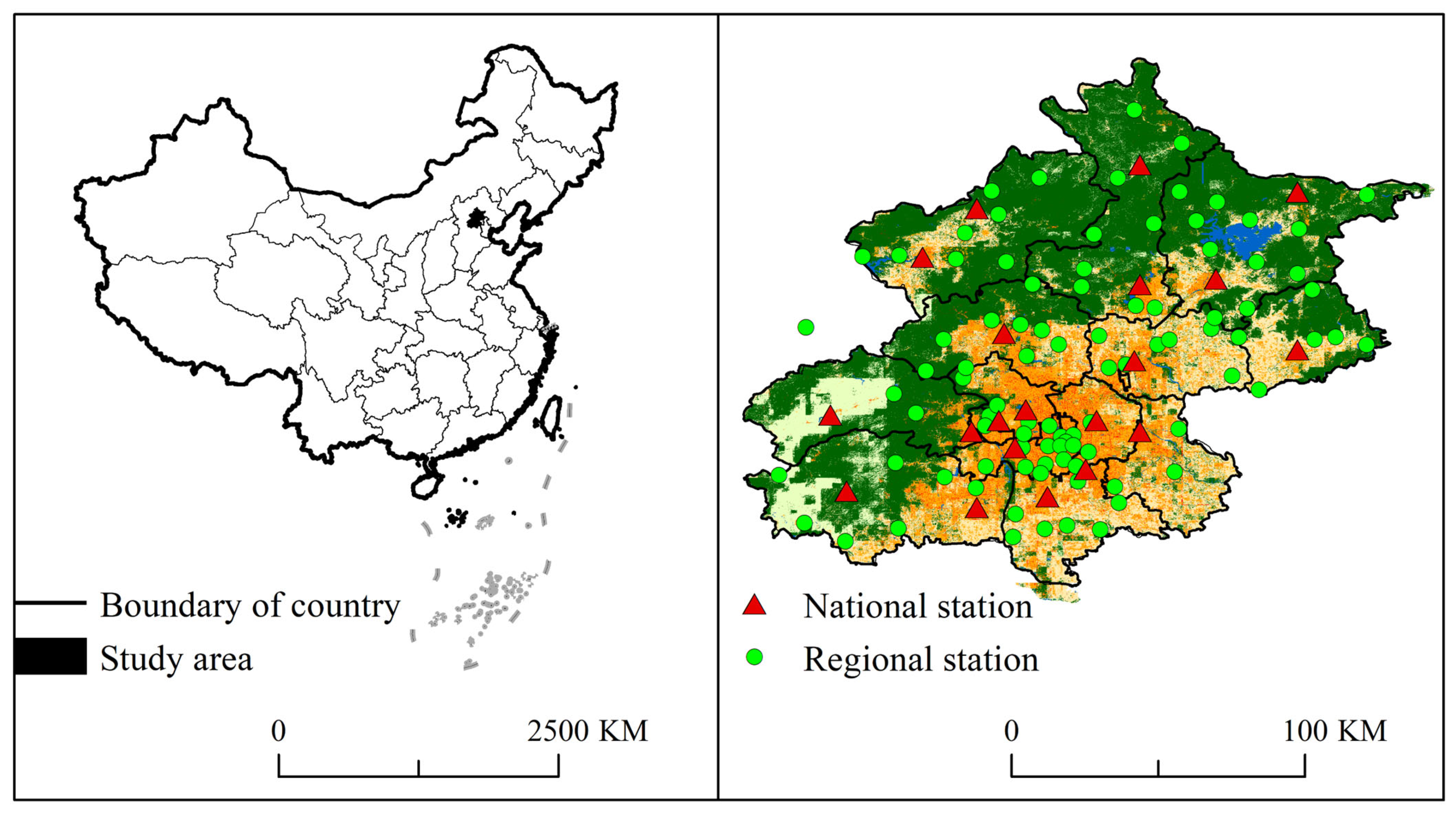
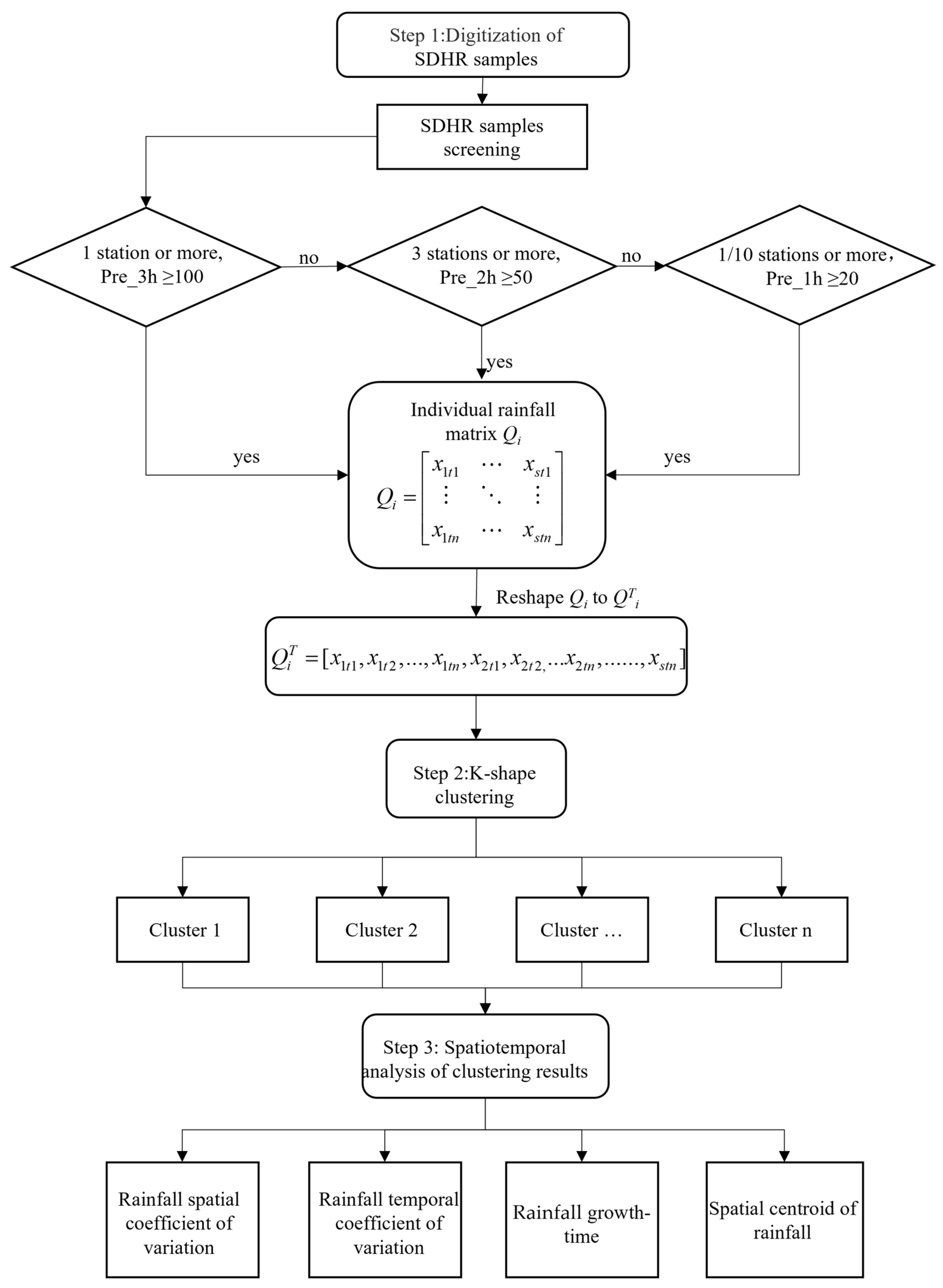
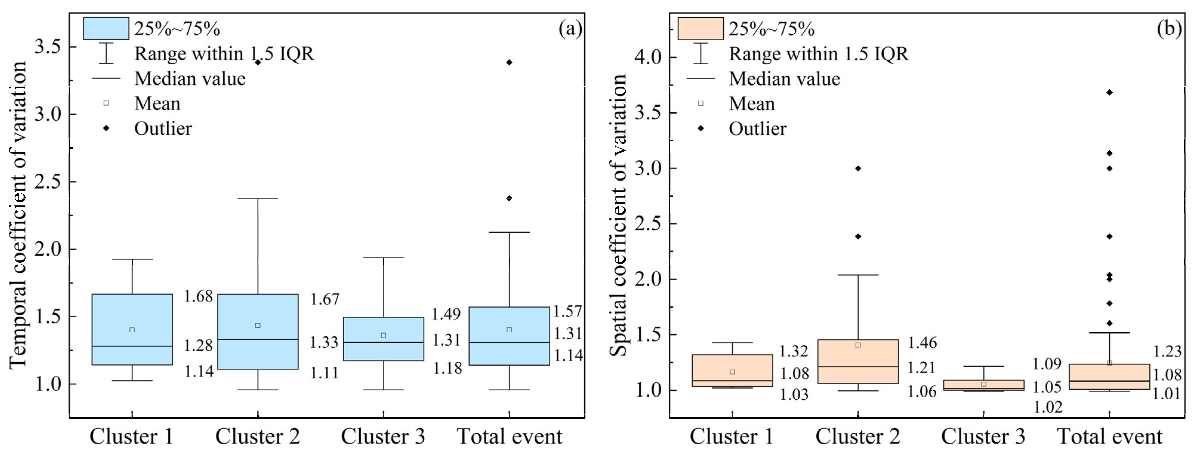
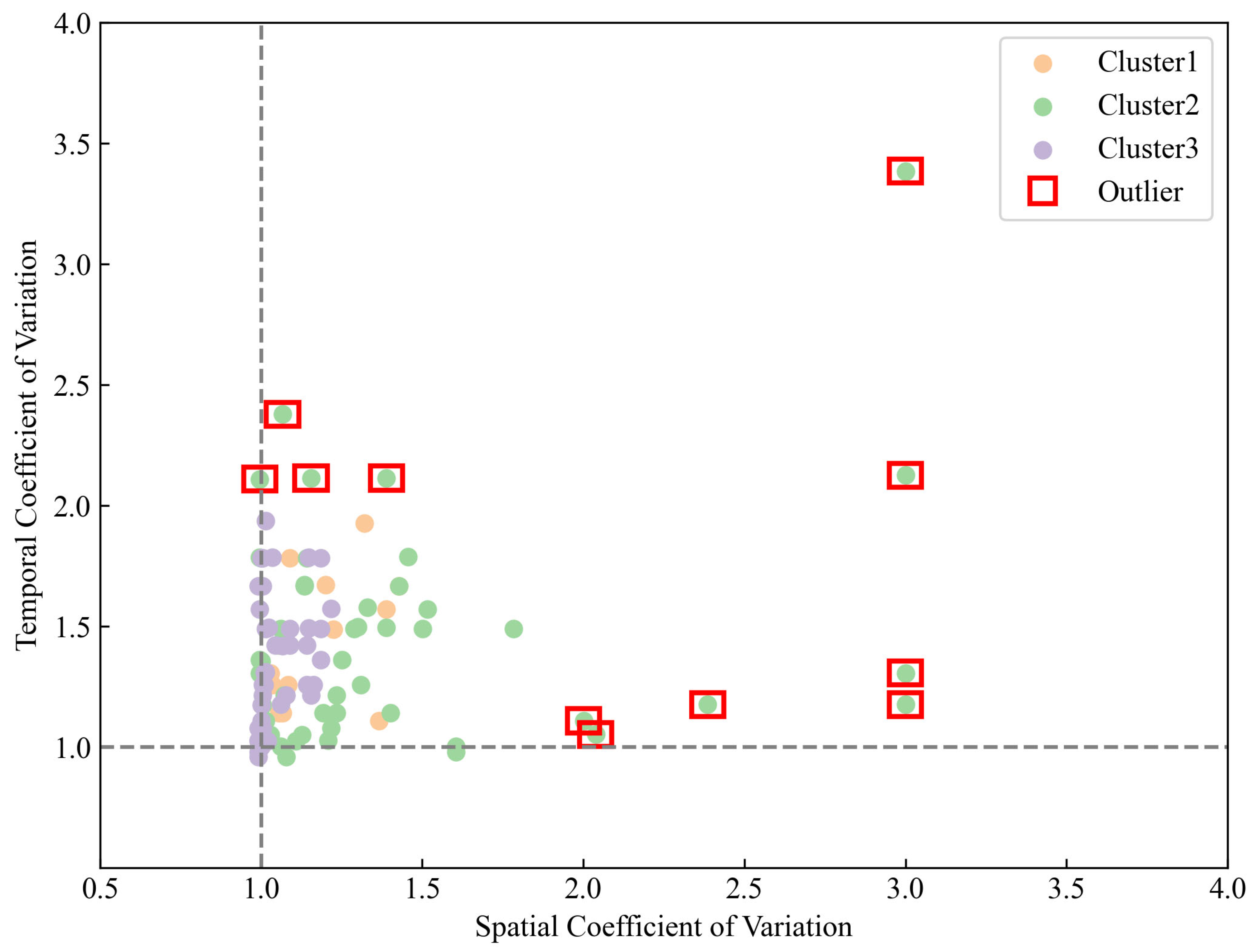
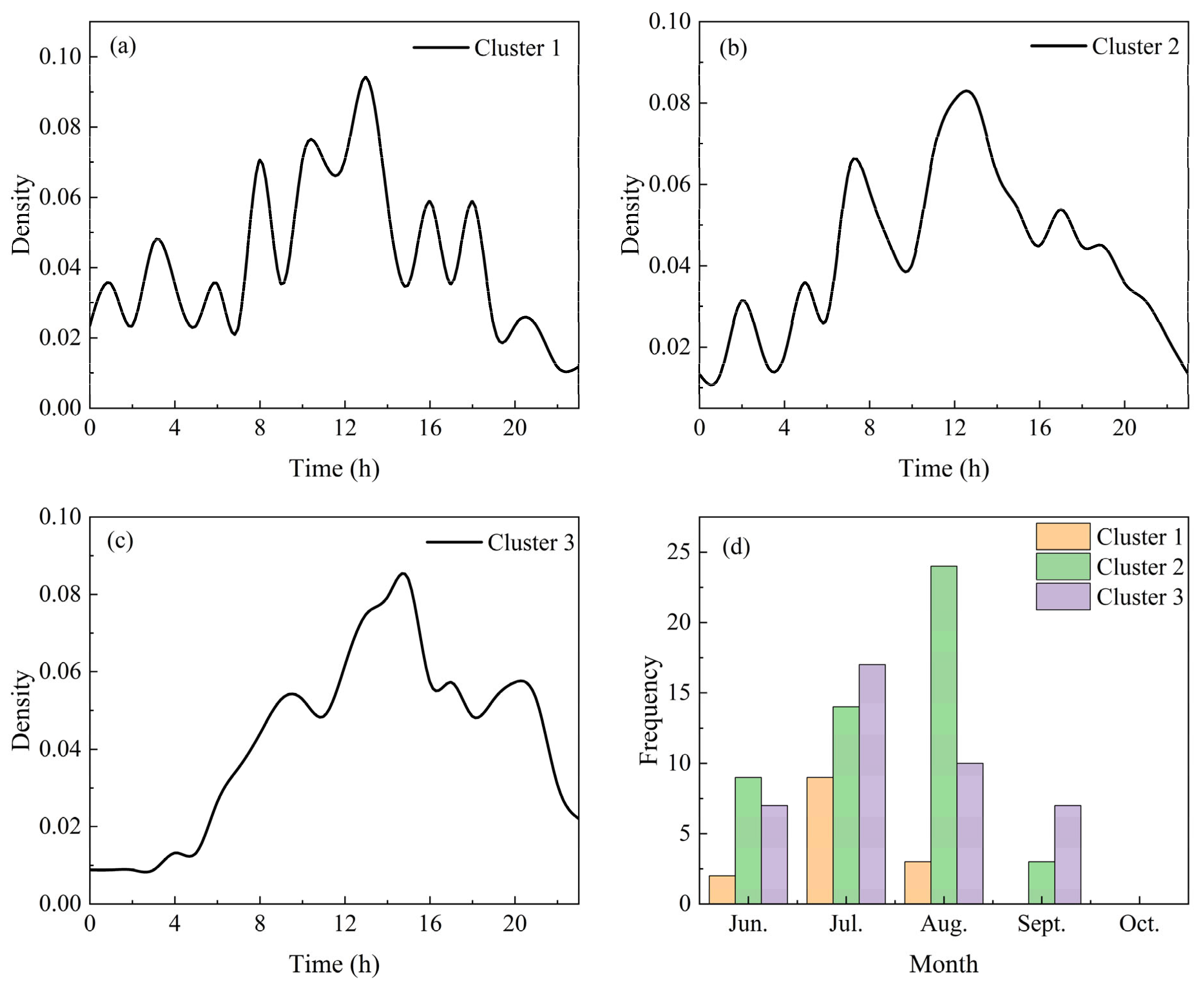
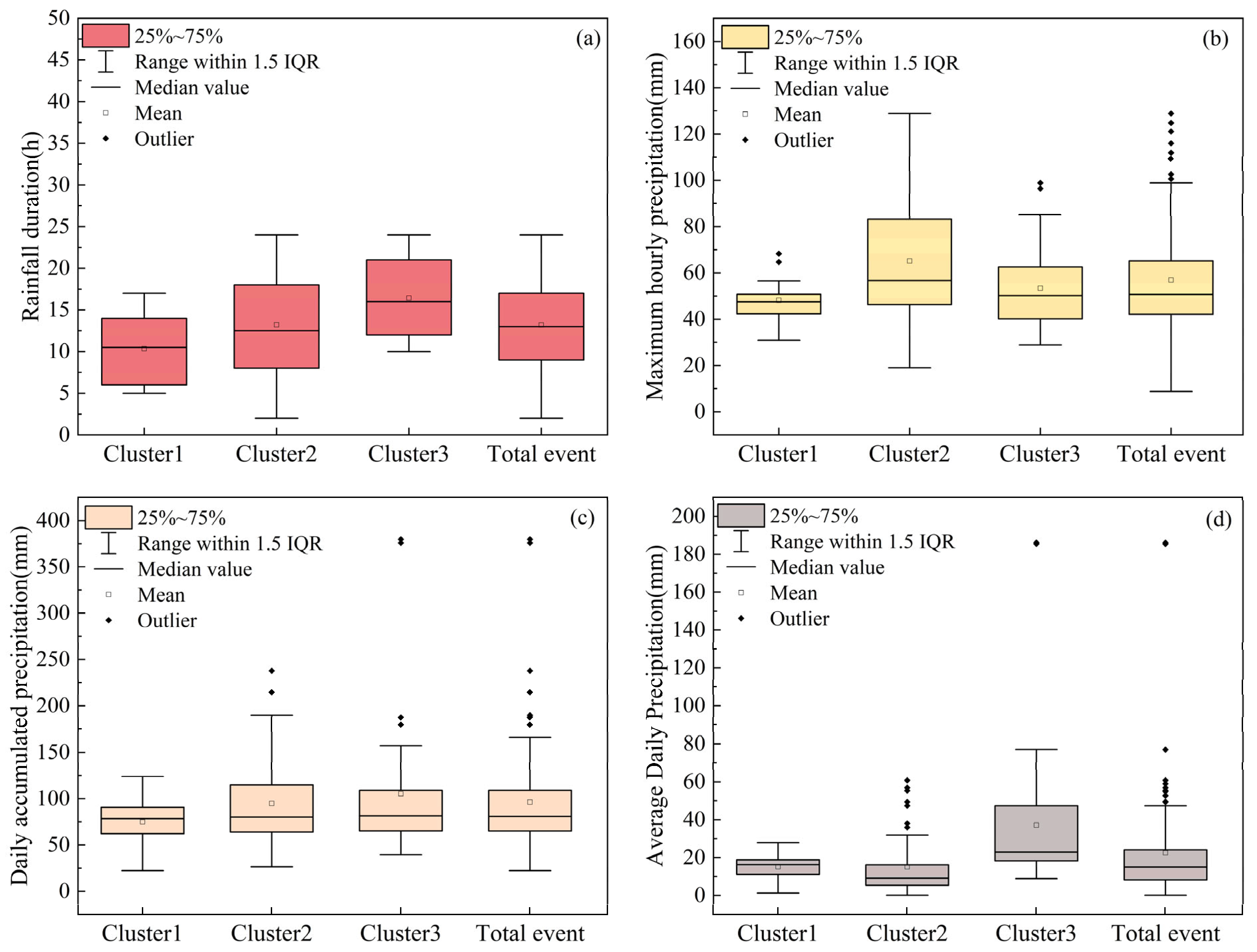
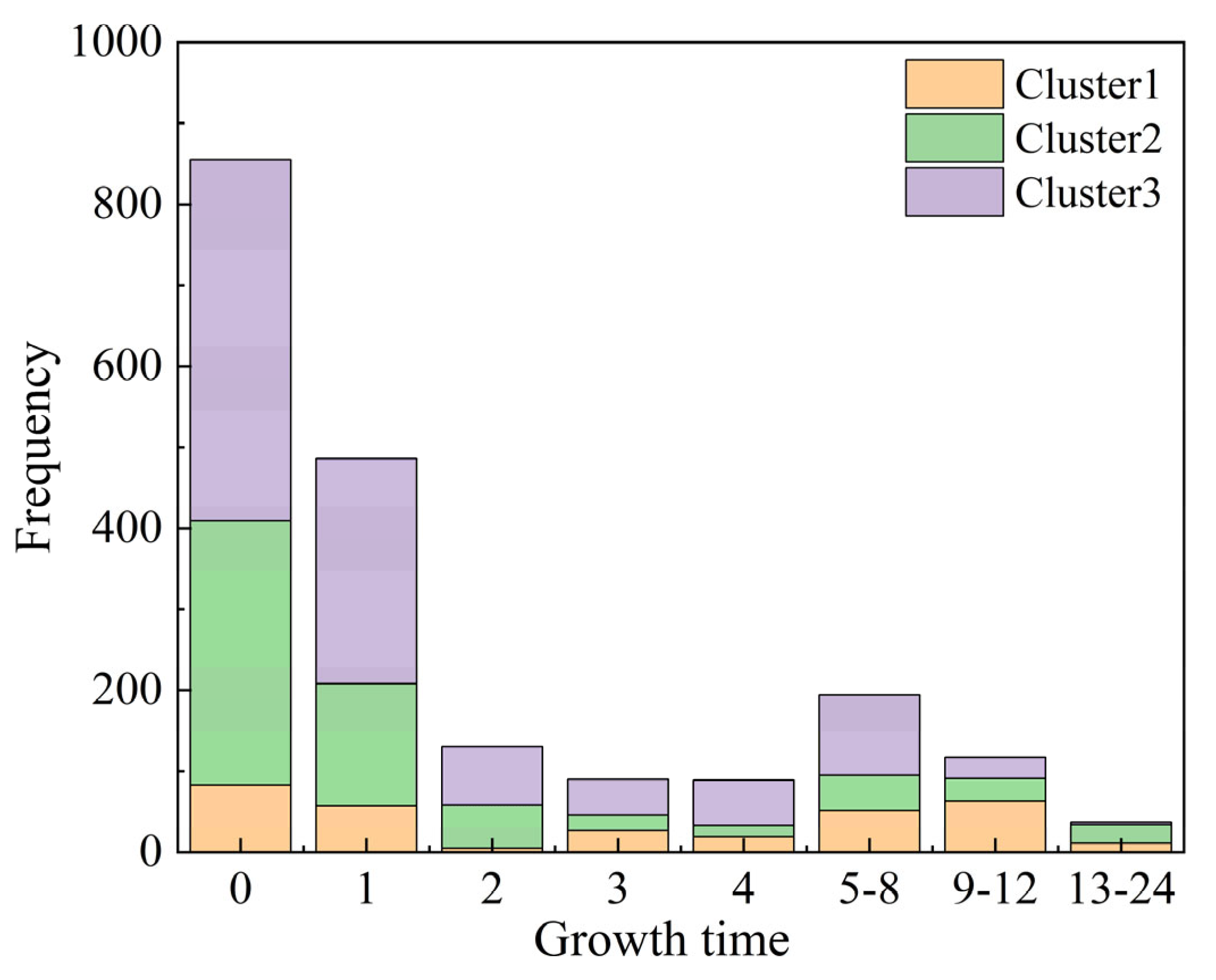
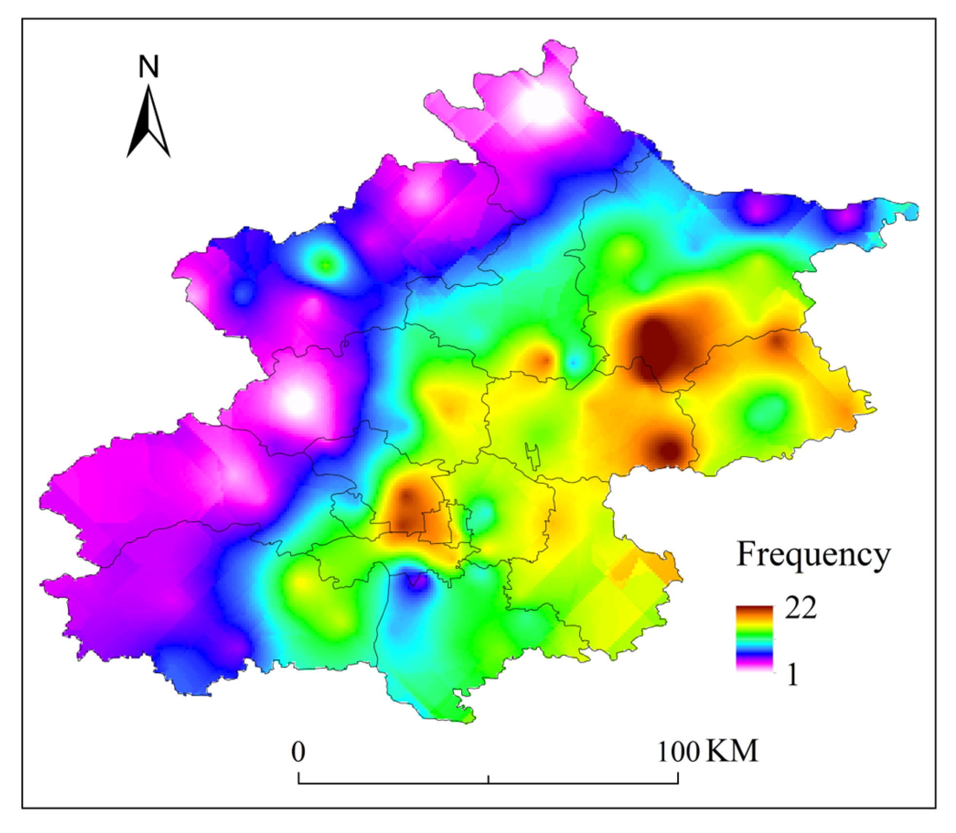
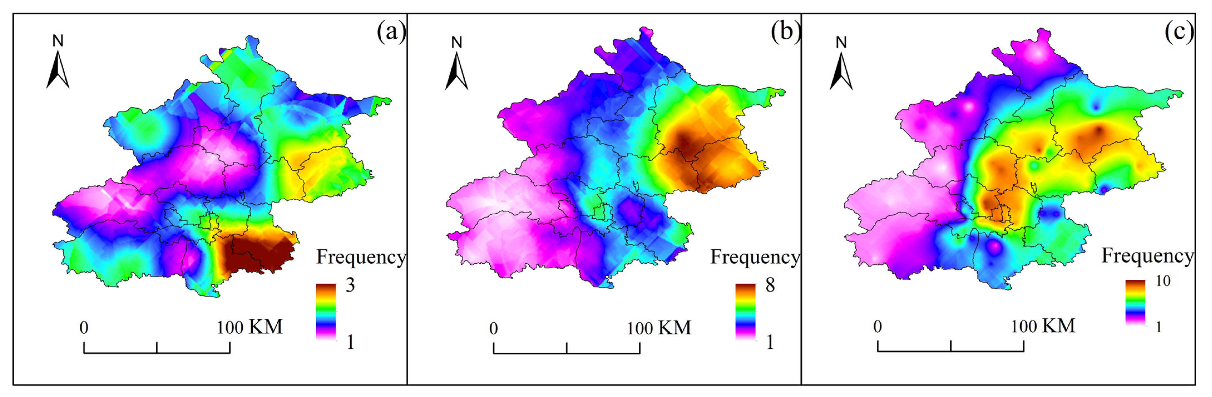


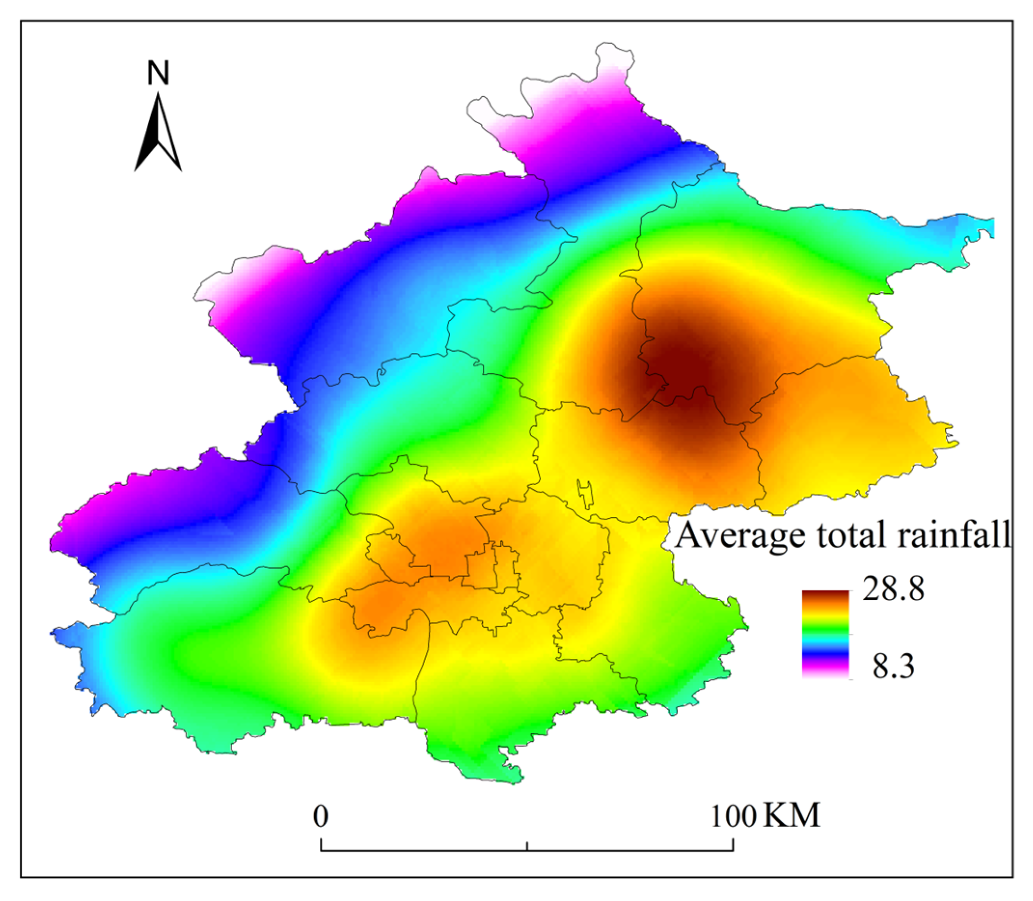
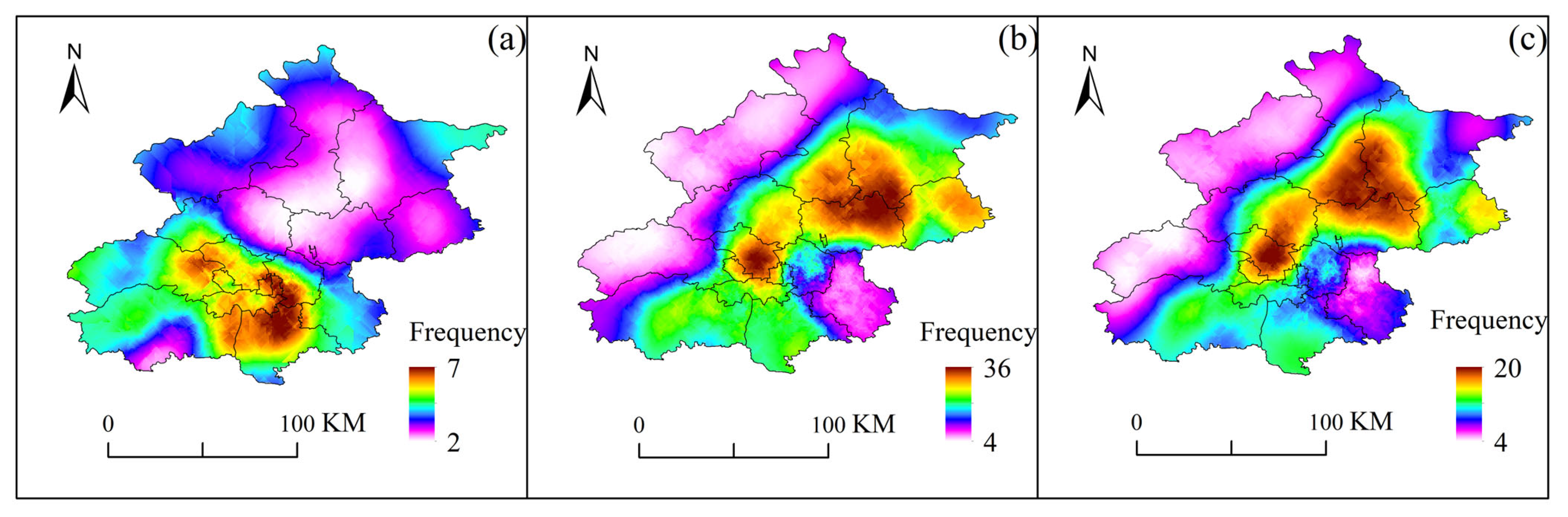
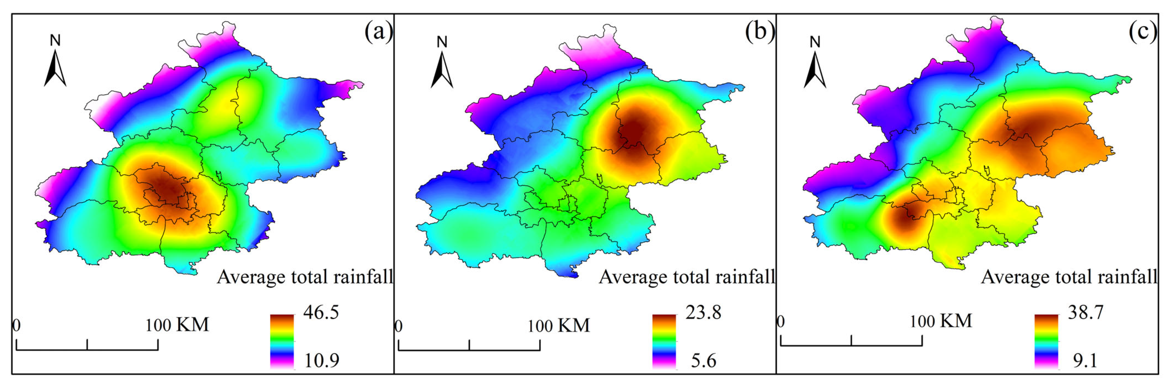
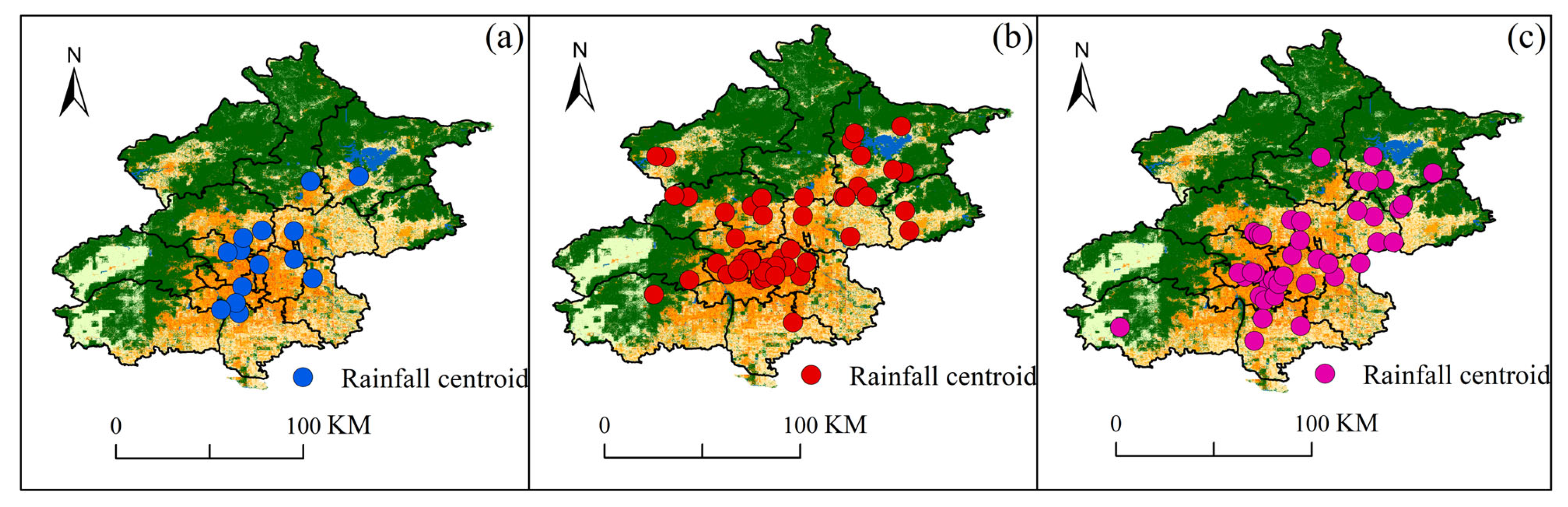
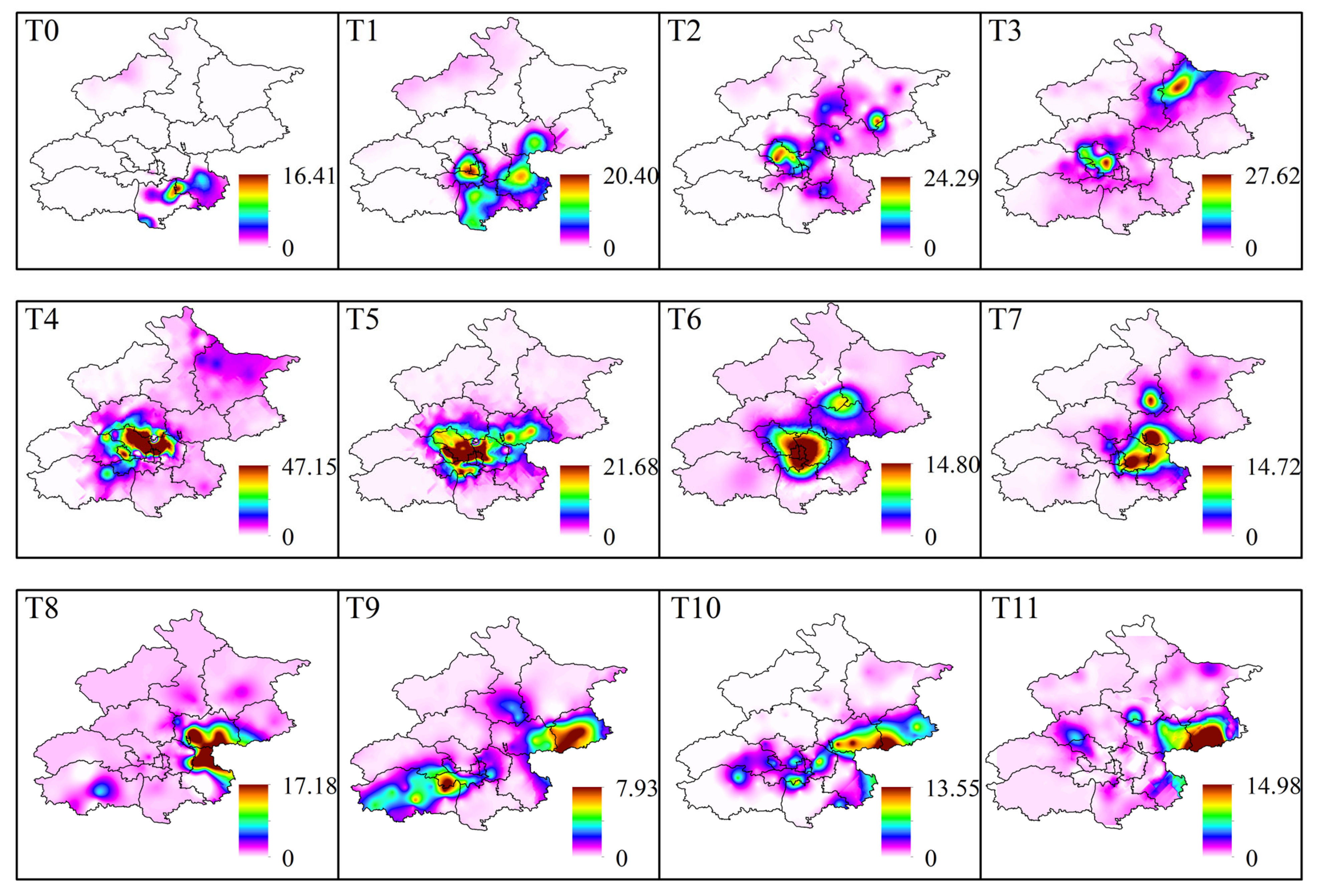
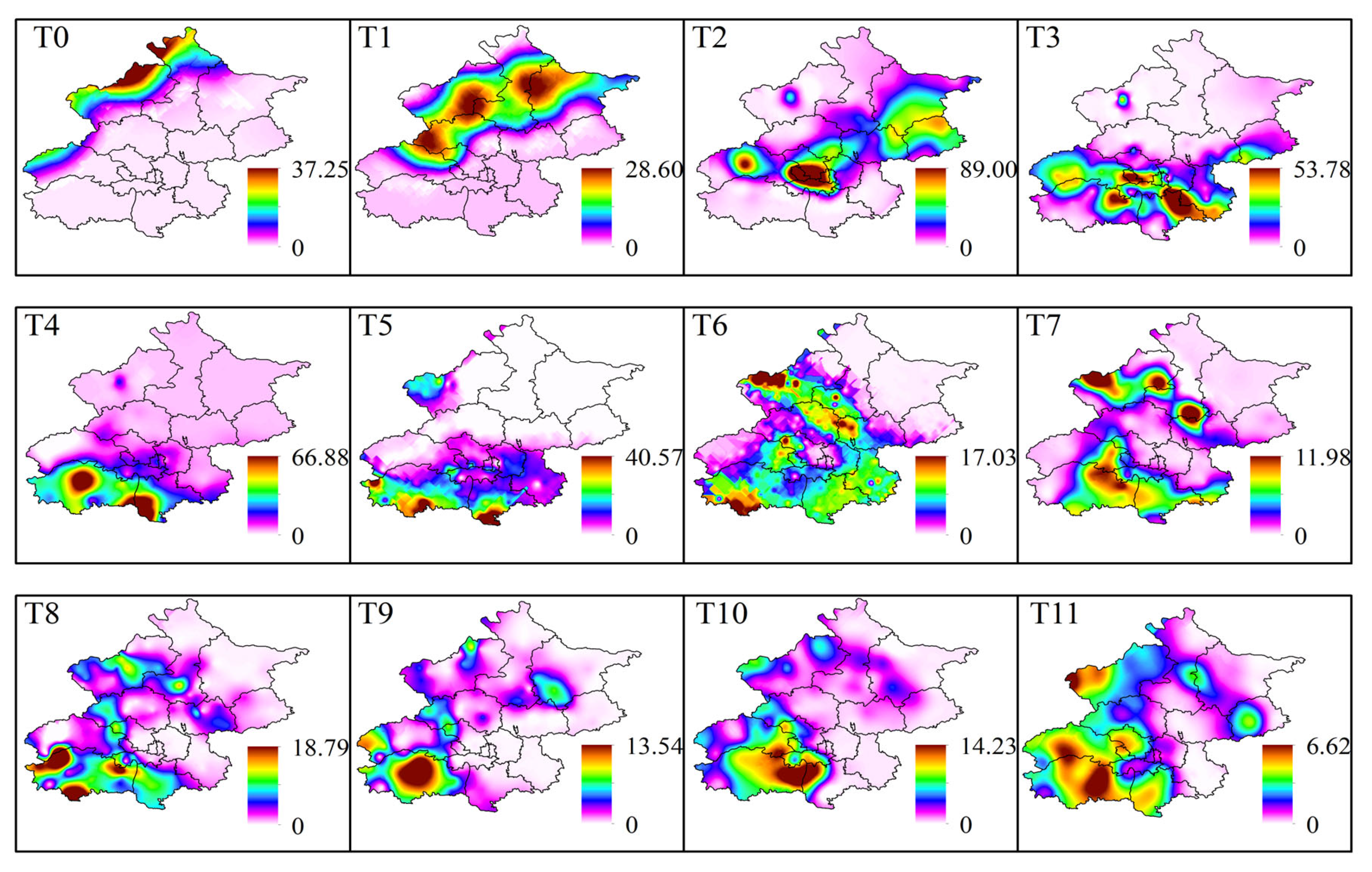

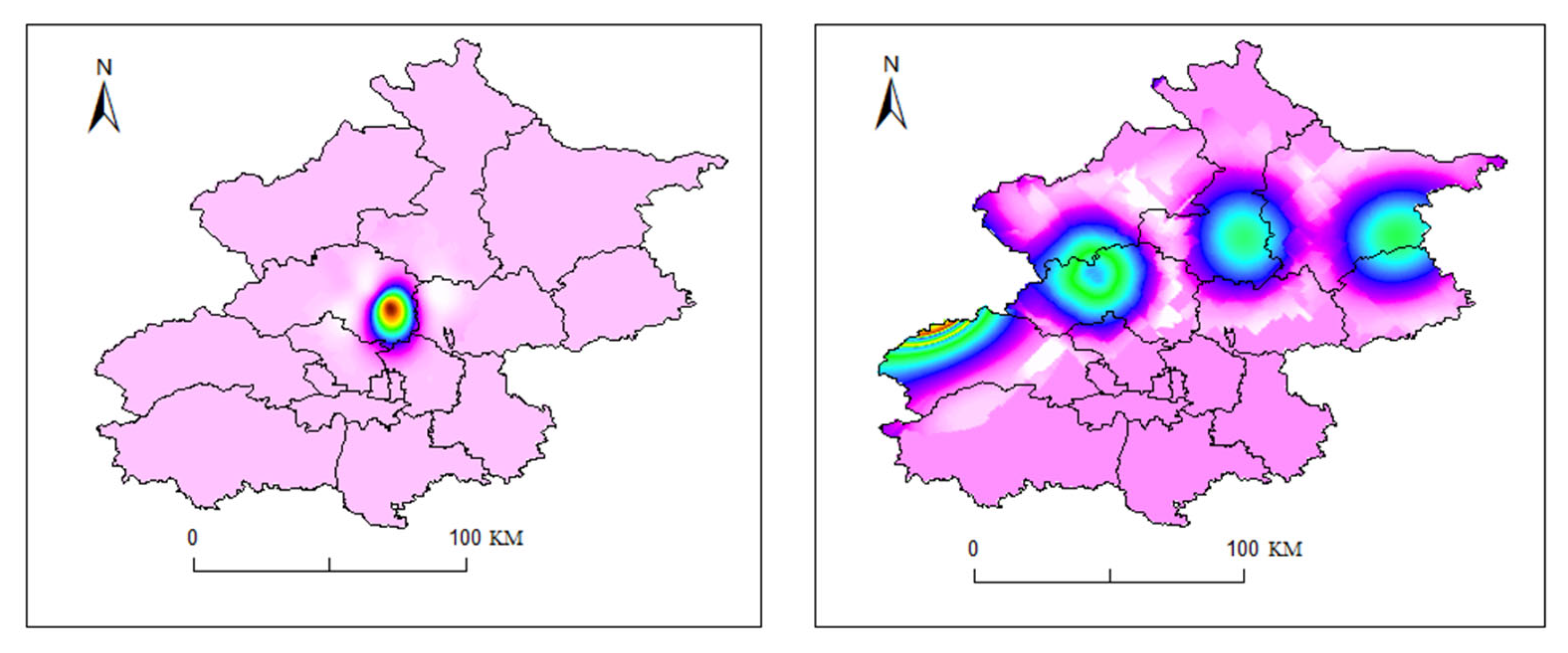

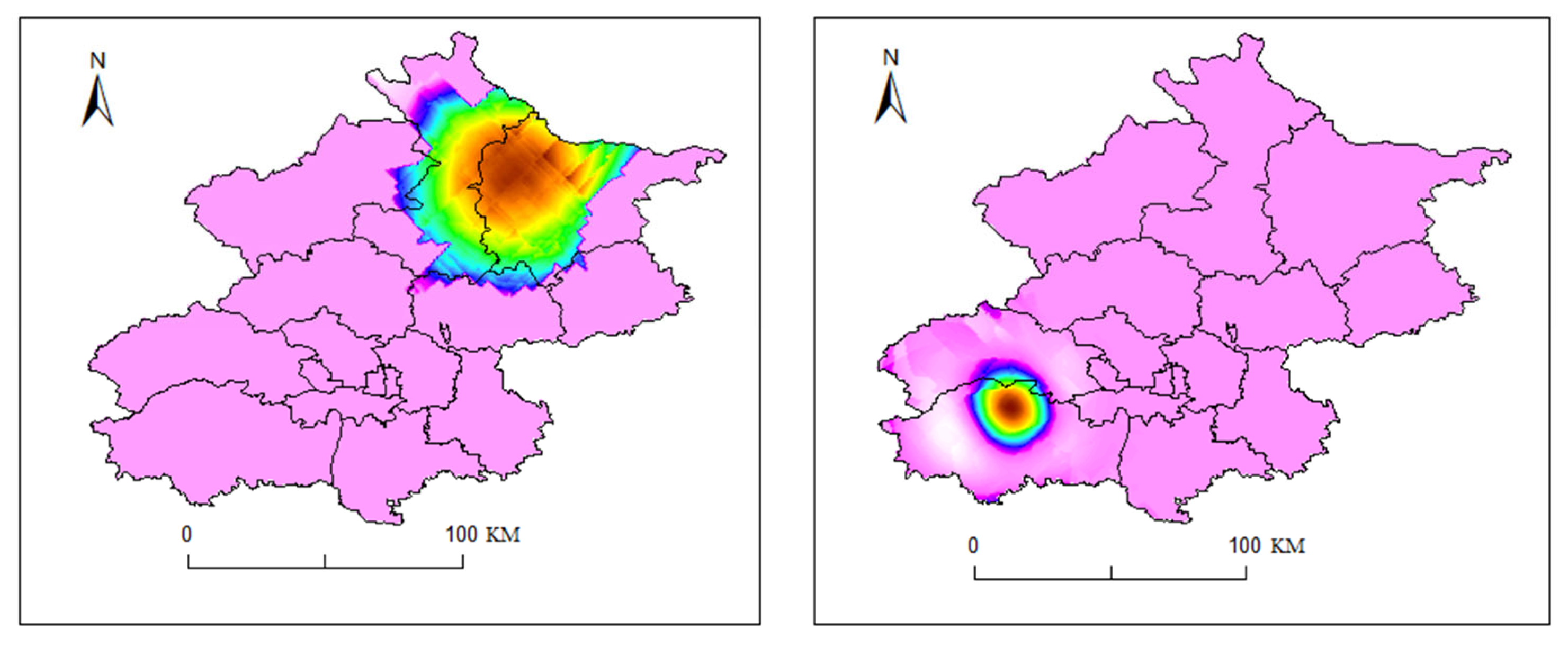
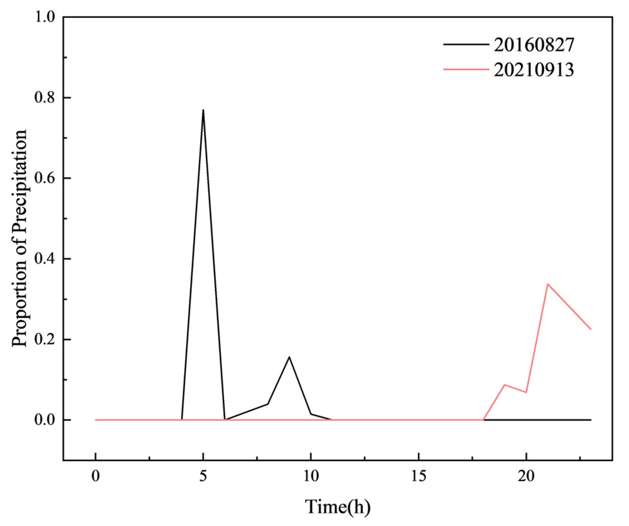
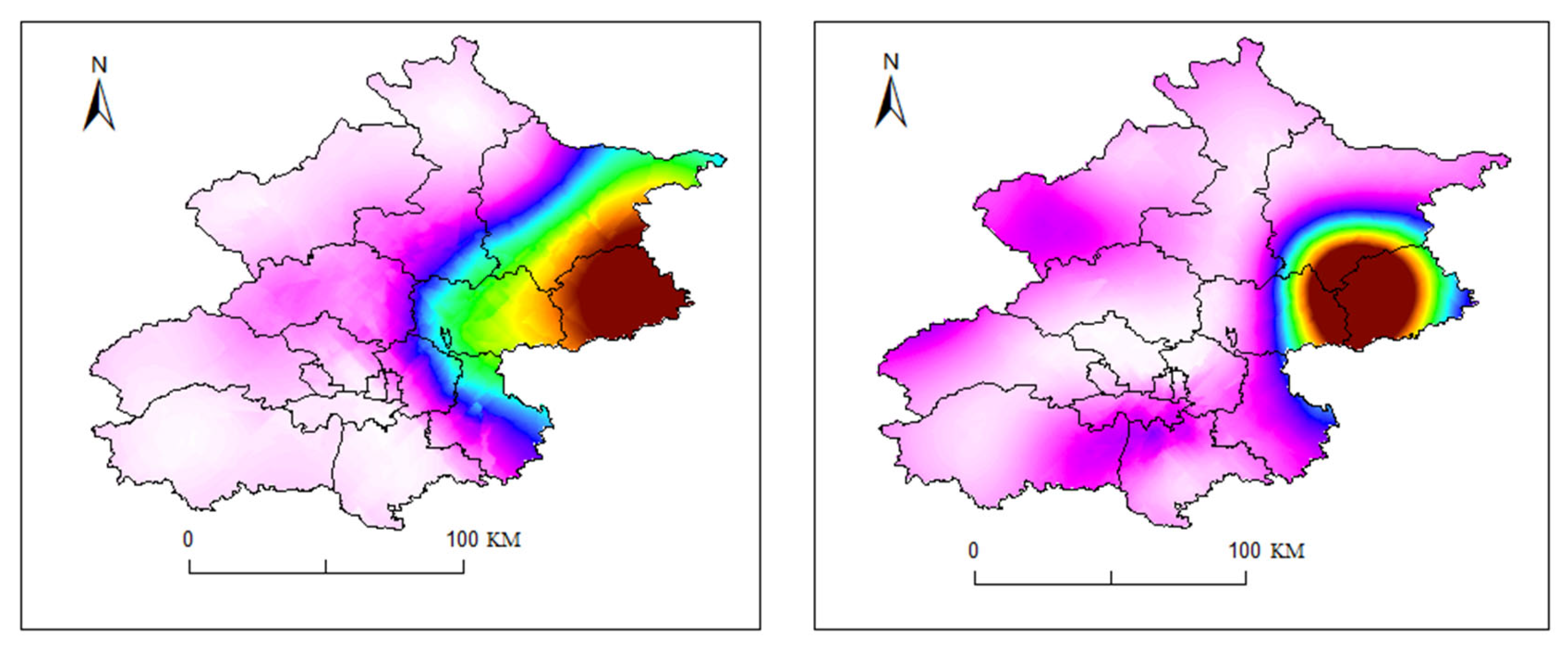
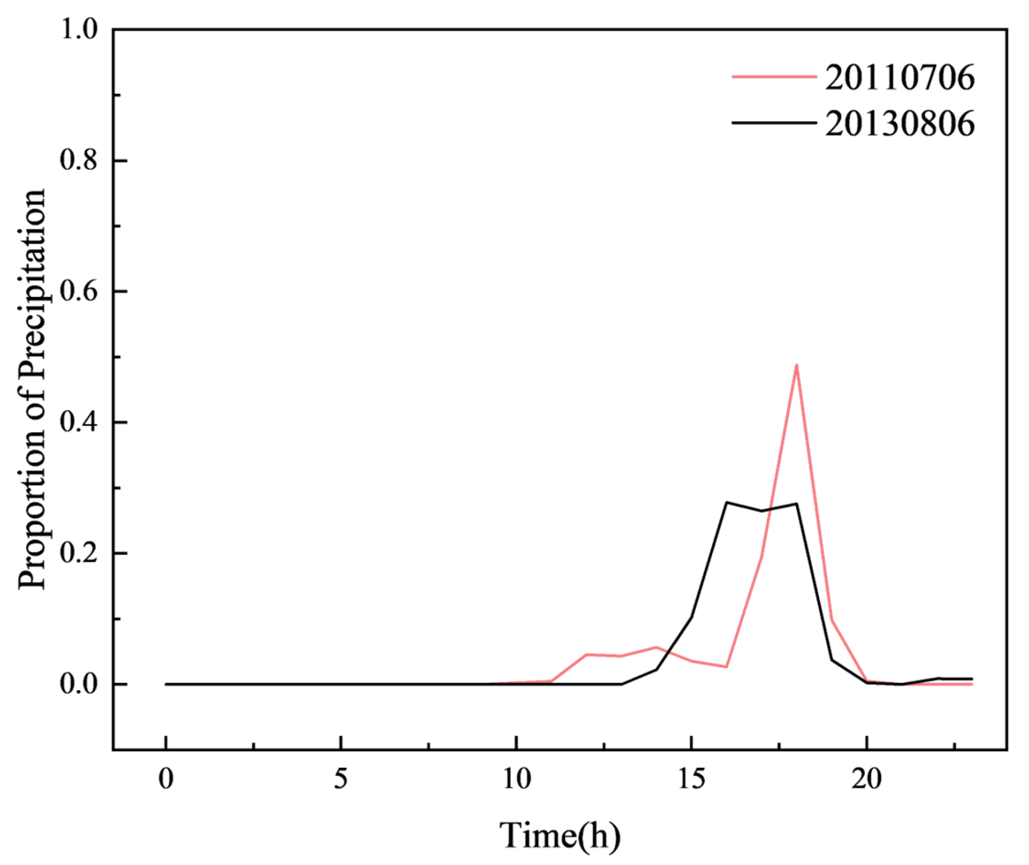
Disclaimer/Publisher’s Note: The statements, opinions and data contained in all publications are solely those of the individual author(s) and contributor(s) and not of MDPI and/or the editor(s). MDPI and/or the editor(s) disclaim responsibility for any injury to people or property resulting from any ideas, methods, instructions or products referred to in the content. |
© 2025 by the authors. Licensee MDPI, Basel, Switzerland. This article is an open access article distributed under the terms and conditions of the Creative Commons Attribution (CC BY) license (https://creativecommons.org/licenses/by/4.0/).