Evaluation of Water Infrastructure System Operation, Partial Productivity, and Their Relationship to Water Loss

Abstract

This study aims to identify areas of opportunity for improvement across selected U.S. water utilities through evaluating system operational performance and productivity and the relationship to water losses. Throughout the water utility industry, there is a need to optimize utility performance as the demand for usable and potable water continues to be a global concern. An analysis of partial productivity and total operating productivity using American Water Works Association (AWWA) data highlights potential areas to improve total water output, minimizing water loss. Productivity relative to water output and losses are also presented showing states and utility sizes with high optimal output based on performance and cost measures. Examined are the management of water operation in California and Georgia water utilities, highlighting the inadequacies and opportunities through an analysis of productivity measurement when compared to water loss. A review of existing literature and data from various sources reveals that both states face substantial challenges in addressing water leakage, despite efforts to mitigate the issue. Research results are presented, showing comparison characteristics and possible future opportunities for improvements.

1. Introduction

Water infrastructure systems are critical components of modern societies, providing essential services to billions of people worldwide. However, these systems are often plagued by leakage, which can have significant impacts on system performance and opportunity cost [1]. In 2018, the U.S. Environmental Protection Agency (EPA) estimated 1.7 trillion gallons [6.4352 trillion liters] of water are lost each year through distribution systems, resulting in a financial impact of approximately $2.6 billion (USD) [2]; a significant contributor to this water loss is the alarming frequency of water main breaks, with an estimated 240,000 incidents occurring annually across the United States, highlighting the need for infrastructure upgrades and proactive maintenance to mitigate these losses and conserve this vital resource [2]. Despite the recognized significance of leakage in water infrastructure system management, the complex interrelationships between leakage, system performance, and opportunity costs remain insufficiently understood, warranting further investigation to optimize management strategies.

Global and U.S. population growth correlates to concerns with future availability of water resource quantity and quality [3]. Even in countries classified as highly developed, there is still a lack of proper water system governance and technical management, which results in an increased cost of implementing improved methodologies [4,5,6]. In the United States, roughly 1.1 million Americans live without running, potable water, including in affluent cities such as Portland, Phoenix, Houston, and New York City [7].

Water available for crop irrigation, for example, has become more limited, and alternate water sources are needed [8]. The same holds true for utility supplied water, from being managed, then processed from the source, to the utility, then to the end-user. A shift in thought from water being readily and easily accessible for all to water being protected and appropriately managed needs to occur [6]. U.S. water and wastewater infrastructure systems continue to age and are well past the original designed service life estimates [9,10] and continues to be a top concern among U.S. water utilities and technical managers [11].

Currently, a gap exists where there is no common applied set of metrics for water utilities to govern and manage performance [4,6]. While the AWWA and Water Research Foundation (WRF) have provided guidance, there is an opportunity to better utilize a common metric set when comparing performance and water loss across similar size water utilities. Many states have decided not to follow this recommended guidance due to factors including lack of awareness, implementation challenges, and the need for significant training and technical expertise required to conduct a proper audit, which can be a barrier for smaller water utilities. This paper introduces the application of a water productivity metric to measure and evaluate water utility performance, including the performance relationship to water utility losses. Water loss within a utility system is expected to negatively impact total productivity, where the higher the water loss, the more the water utility needs to produce to serve its customers (to make up for the loss). This impact led to increased operational and production costs for the utility. The ability to use water loss data and compare both within the state and outside of the state using AWWA performance guidance, in turn, can potentially standardize productivity measurements across water utilities to facilitate comparison and benchmarking.

Water utilities in California and Georgia strive to balance the need for efficient water management with the requirement for affordable water services. Productivity measurements are essential in evaluating the performance of water utilities, as they help identify areas for improvement and inform decision making. With the continued focus on availability of existing water supplies, water resource managers are challenged to improve infrastructure systems and manage internal processes, and productivity measurements can help in this aim. Water research data provided by the United States (U.S.) Environmental Protection Agency (EPA), the AWWA, and the WRF shows opportunities and trends within data utility systems, contributing to reductions in water quantity and quality [12]. Integration of present-day technology into these systems would help increase available water supplies as a sustainable future resource. Examples of such technologies include water leakage detection systems, smart meters, and advanced flow-modulated pressure control tools; with support from the WRF, Halifax Water (Nova Scotia, Canada), was able to implement pressure management tools and strategies that resulted in a 46.9% reduction in water system main breaks and service leaks in the year following adoption [13]. A comparative analysis and discussion within Water Resource Management (WRM) systems, including challenges and opportunities that lie within the system, when properly addressed, could lead to improvement and better management of the utility, to include improved, innovative cost structures in managing the whole water utility system.

The AWWA Water Loss Control Committee (WLCC) has collected datasets of validated water loss audit data from various water utilities in North America. The latest data used as part of this research is from the calendar year 2018 (the data were made available in 2021). The composed and available dataset is called the AWWA Water Audit Reference Dataset (WARD) and shows data from U.S. states (only California and Georgia contain complete datasets) as well as the dataset from Quebec (Canada) [14]. California and Georgia were selected to be part of this research as they all met the requirements defined in the Level 1 Water Audit Validation Guidance Manual, provided by the WRF. In addition, instructions are provided detailing how to document uncertainties, discrepancies, and address other anomalies identified with the data [15].

The most recent, available WARD includes data from 1379 water utilities. As part of the data evaluation for this research, the data were filtered further to avoid skewing of results due to outliers (out of family observations). This filtering removed data from 255 utilities because of potential data errors, duplication, and other out of family data that had been included from the original WARD. After post-filtering the data, the final number of utilities used for the analysis of the dataset, therefore, comes to 1124 (see [14], for detailed audit filtering process). Using data groupings by utility size allows for comparisons amongst similar water utilities based on the population served.

2. Literature Review

The proper and effective maintenance and sustainment of water utility systems and associated services to the customer is dependent on effective, planned technical management processes through technical management and guidelines. The lack of a usable and real productivity system model within the water utility makes it difficult to make effective technical decisions when aiming to change and optimize a system. Blinco et al. [16], performed a study to determine the optimization of pump energy used to move water through a water utility system. The analysis indicated that system energy use showed groundwater and stormwater supplies are more desirable to supplement natural inflows to the utility than the water imported from a nearby river, which required more energy to transfer water over a distance and against high elevation. The established model and framework from that study was generalized and applied to other water supply/distribution systems, especially those using non-traditional water sources, to optimize their system design and operation. The key to that analysis was to use a proper model that accurately portrayed the operation of the overall system, to understand how the whole system was impacted when changes were made.

There are many organizations within the industry that have developed publications and software tools to help in sharing best practices when implementing effective water loss control [4]. The use of the AWWA’s Free Water Audit Software (FWAS) Version 6 (v6.0) helps the capture of data when assessing utility performance [17]. An example of the use and application of the AWWA to assess and compare water loss is found in Horbatuck and Beruvides [1]. The previously mentioned Level 1 WARD data collected use this specific software to support analysis. Additionally, Water Infrastructure Management is cost- and performance-effective when using and applying data from specific studies and water audits, further offering system improvement opportunities [18]. When undertaking and evaluating potential process improvements, it is important to note the items that may be low risk but also provide a low/mid-return.

Numerous studies have examined the relationship between water utility infrastructure system operation and production costs and system output and performance. For example, a study by the AWWA found that water utility operation and maintenance (O&M) costs are significantly influenced by factors such as system size, population density, and water demand [19]. Another study by the Environmental Protection Agency (EPA) found that water utility energy costs are influenced by factors such as system efficiency, water treatment processes, and energy prices [20]. Overall, there is great opportunity within the water utility community to use reliable, available data to review performance measures to identify and drive improvement. The application of these data has been used sparingly on focused WRF projects, but the analysis of AWWA data to review performance measures for improvement has not been found in the literature.

Having useable and reliable water-loss data is critical for decision makers in the water utility industry. Evaluating audited AWWA data to review trends and comparisons aids in identifying gaps and opportunities where planned improvements from prior applied audit data resulted in measurable and positive utility performance improvements. It is also noted that impacts outside of what is captured in the AWWA data can impact the water system; this may include unexpected maintenance costs, aged infrastructure, and administrative challenges. When looking at the system and, in this case, utility performance improvements, the performance measures need to be defined. Use and analysis of the WARD contributes to output measurement (water supplied to the customer, versus water lost). Applying established guidance from both the WRF and AWWA for detailing water use and loss data helps the utility in accurately quantifying system losses.

According to Deming, “Productivity” refers to the system “output divided by input”, and “Effectiveness” refers to the “extent to which the organization [or system] achieves its objectives” [21]. Deming’s philosophy aimed to improve productivity and effectiveness by focusing on continuous improvement, employee involvement, and customer satisfaction [21]. Juran defines “Productivity” as “the ratio of output to input”, and “Effectiveness” is “the degree to which the output satisfies a customer’s needs” [22]. Juran emphasizes the importance of identifying and properly addressing the root causes of problems with effective corrective actions, rather than just treating the symptoms [22].

Both Deming and Juran emphasized the importance of “Efficiency”, which refers to the “ability to achieve a desired result with a minimum amount of waste” [21,22]. Both agreed that organizations should strive to minimize or eliminate waste and optimize processes to achieve greater overall efficiency and productivity. The principles on productivity, effectiveness, and efficiency emphasize the importance of continuous improvement, customer satisfaction, and employee involvement in achieving organizational excellence and system optimization. Sink and Tuttle equate productivity to effectiveness and efficiency, where Productivity = Effectiveness/Efficiency, that is, Productivity is the ratio of Effectiveness divided by Efficiency.

The use of appropriate measures and methods for use in determining performance measurements is important to achieve utility goals, establish distribution efficiency, and ensure water conservation [23]. Within the literature, Sumanth’s [24,25] work in productivity management is centered in understanding total productivity, which also includes the role of technology and work design to drive productivity and performance improvements; this Total Productivity Model considers five key inputs: human, material, capital, energy, and other expenses [24,25]. Sink’s work in productivity and performance management focused on factors that influenced company productivity, with emphasis on work design and leadership [26]. Sink and Tuttle later defined a model that includes seven criteria in the performance of an organizational system; Effectiveness, Efficiency, Quality, Productivity, Quality of Work Life, Innovation, and Profitability [27]. In addition, and using the above criteria, Sink and Tuttle [27] discuss where organizations should focus in areas to include Performance Measurement, Performance Improvement, Planning, and Control. Measurement in these areas will help track performance and identify areas of improvement. Noted, an identified gap in the literature, and specifically Sink and Tuttle’s model, includes a limited amount of focus in the environmental area [28]. However, a published master’s thesis noted the Sink and Tuttle gap and a measure was identified to include the environmental piece and a supporting model [29].

When it comes to water loss, the water system input efficiency will impact the system output (or effectiveness of revenue water, where revenue water is defined as water billed to the customer). The overall water system’s measure of productivity is defined as revenue water/system input (or more generally, output/input). For the system, non-revenue water (or water loss) is identified as waste and contributes to the system’s total output. As many water utility systems are revenue generating, any water loss is expected to negatively impact the system productivity by increasing overall utility cost.

In the context of water resource management, the aforementioned principles can be applied to improve the efficiency, effectiveness, and productivity of water utilities, thus, providing a basis for water utilities to improve operations, reduce waste, and enhance customer satisfaction. From the data provided, the general hypothesis is that the water utility operating and partial productivity measurement shows an inverse relationship when compared to utility water losses. Specifically, as the utility operation and partial productivity metric increases, water utility losses (Infrastructure Leakage Index (ILI) value) is expected to decrease.

3. Research Objectives and Data

California, known for its drought-prone climate, has been at the forefront of water conservation efforts. The state has made improvements in trying to advance water loss management, including CA Senate Bills 555 (2015) where legislation was updated to require water suppliers to submit water loss audits annually, whereas the previous requirement was every five years [30]. In addition, in 2015, California formed the Water Loss Control Collaborative to allow for improved partnership on planning improved water loss control and includes utility personnel, industry organizations, consultants, non-profits, and state entities. However, the state’s water utilities still face significant challenges in managing water leakage. A study by the California State Water Resources Control Board (SWRCB), estimated 20% of the state’s potable water supply is lost due to system leaks and other inefficiencies [30]. The Los Angeles Department of Water and Power (LADWP), one of the largest water utilities in California, reported an average annual water loss of 12.5% between 2015 and 2020 [31].

Georgia is another state that faces challenges in managing water leakage. Georgia started to require public water systems to implement water loss control programs on 1 July 2016, and included audits that must be conducted using AWWA methodology and submitted to the Georgia Environmental Protection Division (GEPD) [32]. The activities within the water loss control programs include leakage management, meter testing, and preventive maintenance. The GEPD also created a Qualified Water Loss Auditor (QWLA) certification program in 2015, which the Georgia Association of Water Professionals (GAWP) administers [32]. A study performed by the Georgia Environmental Protection Division (GEPD) assessed an average of 15% of the state’s potable water supply is lost due to leaks in the water system [32]. The City of Atlanta’s Department of Watershed Management, one of the largest water utilities in Georgia, reported an average annual water loss of 10.5% between 2015 and 2020 [33]. Both of these measures justify the need for a water loss control program.

The relationship between the operation and production costs of California and Georgia water utilities and their system output and performance is complex and influenced by various factors. According to the California SWRCB, the state produces a system output of 34.6 billion gallons [130.975 billion liters] per day (BGD) (Note: AWWA data are provided in U.S. gallons and miles; the equivalent SI values are in brackets, [1 gallon = 3.78541 L]); Georgia water utilities, on the other hand, have a system output of 23.4 BGD [88.579 billion liters per day] [32].

Considering that governance practices for water management, funding of new projects and improvements, and the availability of auditable data to highlight system performance vary across states and regions, this research proposes the following:

• Use AWWA provided WARD to evaluate system productivity across and within California and Georgia state groupings, by employing specific data on Total Annual Operating Water System Costs (TAOC), Production Costs (PC), and system revenues;
• Analyze the above productivity measures to identify system characteristics driving significant performance differences to present improvement opportunities to better manage the utility system. This includes the evaluation of the relationship between productivity measures and water loss.

Conducting a comparative analysis of operations and partial productivity, considering factors like facility size and water loss, can identify top-performing facilities and inform benchmarks to improve the efficiency of similar utilities. The use of industry data obtained from the AWWA will help identify theoretical as well as the operational characteristics impacting productivity of the system resulting from infrastructure interruptions or failure. Any potential identified return on investment (ROI) to the utility based on the data analyzed will be shared.

Specifically, this research includes exploration of the relationship between operating and partial productivity and facility size, as well as the relationship between these productivity measures and water loss. The division of utilities into “small” and “large” groups was established using EPA guidance [12,34] and based on previous studies with this dataset [1]. Several other factors may impact economies of scale in water utilities, including water source types, demand concentration, and the capital-intensive nature of the industry; however, specific data supporting these variables were not included in the WARD, and they are, thus, outside the scope of this analysis. Specific to the data included in this analysis, it is expected the states evaluated will demonstrate lower relative operating and production costs at larger facilities due to better overall funding and system control, including less total water loss, leading to higher utility performance when compared to smaller facilities. It is also expected that facilities with higher water losses are expected to have lower productivity, regardless of size, due to the corresponding decrease in customer-billed revenue. As a result, productivity is likely to be inversely related to water loss. Therefore, the testable hypotheses guiding this research are stated as follows:

• Hypothesis 1: Operating and partial productivity measurements at small and large facilities shows a difference in productivity when compared within and across the states;
• Hypothesis 2: The state of California’s Water Utility operating and partial productivity measurement at small and large facilities shows an inverse relationship when compared to utility water losses;
• Hypothesis 3: The state of Georgia’s Water Utility operating and partial productivity measurement at small and large facilities shows a more significant inverse relationship when compared to utility water losses.

It is believed that increased funds from the customer aid in appropriately funding projects to maximize production output, minimize variation, and heighten utility performance. When higher water losses are observed, the inverse relationship between water losses and utility profit would be more significant. In addition, it is believed that large utilities are better funded compared to small, and overall California better funded compared to Georgia. While Georgia utilizes recommended AWWA controls, California maintains stricter water loss controls through funding of various programs on Level 1 water audits [1]. California also has customer water rates that are closer to what is being supplied to the customer and less total water loss when compared to utilities in the state of Georgia [1]. Both states maintain different water management policies, which will also be reflected in the inverse relationship when comparing across states. The methodological approach in identifying state groupings is further described in Horbatuck and Beruvides [1] in taking population served groupings using U.S. EPA guidelines.

This research seeks to understand the varying performance levels among water utilities, focusing on factors such as operating costs and productivity, and utility investment return. The paper will also reinforce the need for streamlined governance at the utility, where useable, auditable water data can help drive technical manager decision making, leading to utility operational, cost, and performance improvements.

4. Methodological Approach

The high-level analytical approach to this research will use the AWWA WARD [14] and will follow the methodological flow as outlined in Figure 1, below. The methodologies applied as part of this research will also include the use of the AWWA Water Audits and Loss Control Programs Manual of Water Supply Practices—M36 [35]. The research scope will include utility costs, customer billing, and water loss data, and system performance and output data from U.S. states Georgia and California. This comparative analysis using the AWWA Level 1 Audit data will aim to address the research gap in the literature and define a measurement approach to analyze productivity, effectiveness, and efficiency data within the systems identified. The methodologies applied will also be used to analyze productivity within the context of specific variables, including utility size and water loss.

Applying the productivity measurement discussed earlier, the productivity measure for this study requires both an output (effectiveness) metric and an input (efficiency) metric. In the model, efficiency is an input to productivity because improving resource utilization and minimizing waste will allow for greater system output with the same amount of input, therefore, directly contributing to higher productivity levels.

To establish the Output metric, first, a Customer Billed Revenue (CBR) is calculated from the AWWA dataset by taking the Customer Retail Unit Cost (CRUC, in U.S. dollars (USD) per 1000 gallons [3785.41 L]) from the WARD and multiplying it by the sum of the utility’s Billed Metered Authorized Consumption (BMAC) and Billed Unmetered Authorized Consumption (BUAC). That is:

Output = (BMAC + BUAC) × CRUC,

(1)

Then, two different input metrics are identified to allow the calculation of Cost Productivity for both the utility Production Cost Value (the partial productivity measure) and the Total Annual Operating Water System Costs (TAOC) (a measure most analogous to total productivity). Input data includes the cost the utility incurs to produce or generate water revenue. These costs may include labor, materials, capital, energy, or service. Specifically, for the purposes of this study, Production Cost and TAOC are defined as follows:

• Production Cost—focuses on variable costs, which are the expenses that fluctuate with the volume of water produced; examples of associated costs include raw water, energy used in production, treatment costs. Productivity Value is calculated by Water Supplied × VPC;
• TAOC—all expenses with running the utility, including Production and fixed costs; examples include salaries, overhead, maintenance, and insurance costs. The TAOC is an existing variable in the WARD.
• As noted above, the productivity measure that uses TAOC is most analogous to what is referred to in the literature as total productivity as TAOC attempts to capture most (if not all) operating costs; whereas Production Cost is a subset of TAOC, and, thus, the productivity measure that uses Production Cost only is a partial productivity measurement. The full equations for each productivity measurement are as follows:

Partial Productivity = ((BMAC + BUAC) × CRUC)/(Water Supplied × VPC),

(2)

Total Productivity = ((BMAC + BUAC) × CRUC)/TAOC,

(3)

When evaluating the Productivity metric, the results aim to see where the utility is performing well and also areas where there exists an improvement opportunity to focus effort, time, and cost factors. Since Total Productivity is measured as a ratio, generally, a Total Productivity score of 1.0 or greater indicates a positive productivity score, where a number under 1.0 indicates there may be areas to improve. As public water utilities are typically not-for-profit entities (managed by local governments or municipalities), values greater than 1.0 are not necessarily expected, and values slightly less than 1.0 may also be indicative of strong performance depending on the specific context (e.g., the existence of other funding to supplement revenue generated through customer billing). Partial Productivity is more difficult to evaluate as absolute benchmarks (e.g., 1.0) may not exist. Partial Productivity values much larger than 1.0 are expected for most contexts, and they are often most meaningful in comparison to other similar entities and in examining trends over time.

For the evaluation of water losses, each utility has an identified Water Infrastructure Leakage Index (ILI) as part of the WARD. The AWWA calculates this as the ratio of Current Annual Real Losses (CARL) to Unavoidable Annual Real Losses (UARL) (which are both also variables in the WARD) as follows:

ILI = CARL/UARL,

(4)

Being a ratio, the ILI has no units and, thus, facilitates comparisons between countries that use different measurement units. The ideal ratio for ILI is 1.0, where the system’s actual losses would match the estimated, expected, or planned loss. UARL represents the theoretical minimum water loss that can be expected even with optimal leak detection and repair practices. Loss which is over and above the normal loss is an abnormal loss.

Unavoidable Annual Real Losses (UARL) is calculated using a formula that takes into account factors like the length of water mains (Lm, in km), the number of service connections (Nc), the average system operating pressure (P), and the length of service lines (Lp, in km). This formula estimates the minimum amount of water loss considered unavoidable even with well-maintained infrastructure; the basic equation used by the AWWA is:

UARL (m³/year) = (6.57 × Lm + 0.256 × Nc + 9.13 × Lp) × P,

(5)

5. Results

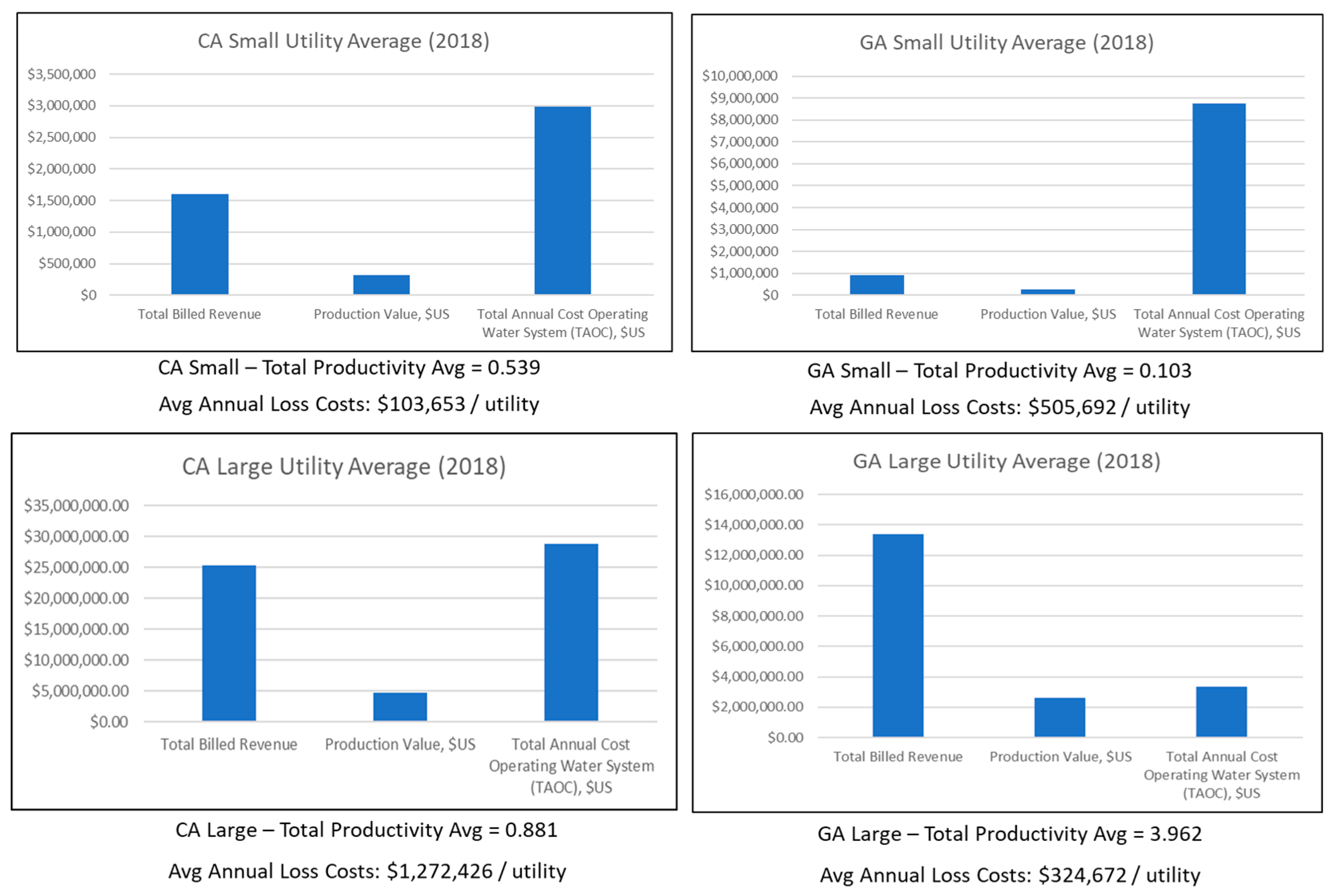
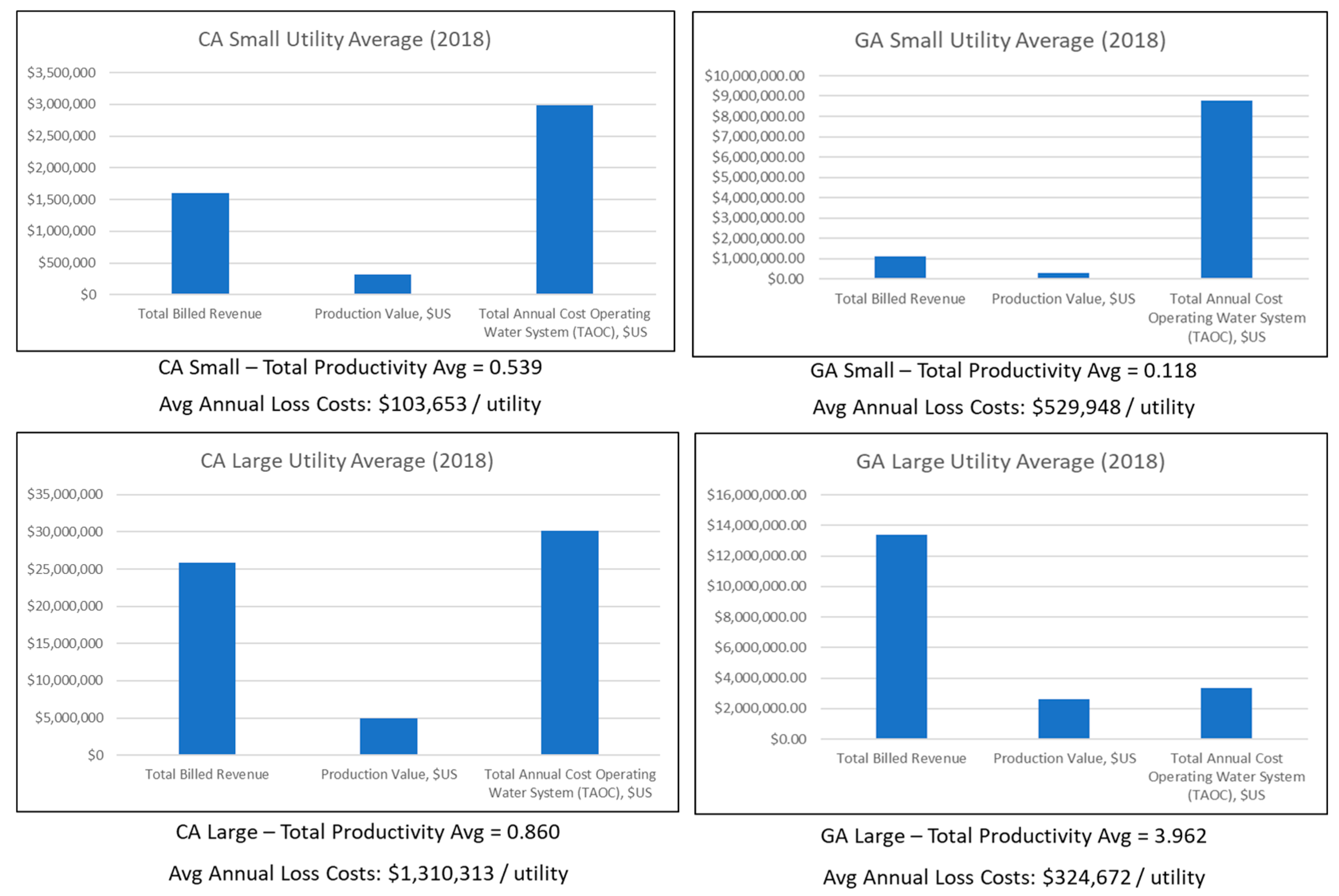
The analysis began by numerically and graphically comparing Total Productivity and Partial Productivity and their component metrics (Customer Billed Revenue, Production Value, and TAOC) by state facility size groups identified in Section 3 (Figure 2). The results showed a large variation and some unexpected behaviors (Standard Deviation and Interquartile Range (IQR) values displayed in

Table 1. CA and GA Average Revenues and Cost Comparison with Standard Deviation and IQR.

Group	Standard Deviation	IQR Value
CA Small
Total Billed Revenue	$860,081	$1,231,932
Production Value	$491,583	$413,817
TAOC	$1,589,552	$1,865,517
CA Large
Total Billed Revenue	$79,880,999	$20,251,942
Production Value	$1,215,141	$917,162
TAOC	$83,559,252	$22,788,896
GA Small
Total Billed Revenue	$780,154	$979,737
Production Value	$376,952	$209,264
TAOC	$23,053,342	$4,571,027
GA Large
Total Billed Revenue	$28,829,240	$7,179,782
Production Value	$7,714,504	$1,663,522
TAOC	$5,476,504	$2,510,453

). For instance, in the GA large grouping, the average Total Productivity value was close to 4.0 (i.e., Billed Revenue greatly exceeds TAOC), which is unexpected for not-for-profit operations. Meanwhile, the reverse was true for the GA small grouping, where the average Total Productivity was unexpectedly low (close to 0.1), even for not-for-profit-operations. To account for potential outliers (out of family observations), which could be driving this, there was an initial attempt to filter the Total Productivity values using the + 3-sigma method; however, when this was completed, no significant differences in the results were observed. 3-sigma was initially chosen as this is the standard measurement used in water quality control [36,37].

Next, the data were plotted, establishing both a total operational productivity metric and a Production Value metric, both compared to the utility ILI. The results are plotted in the below figures, across both California and Georgia and by small and large state groupings.

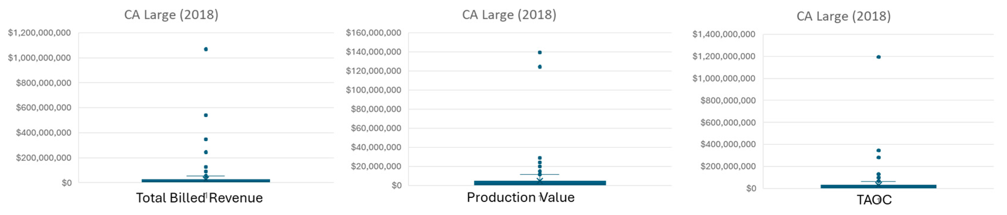
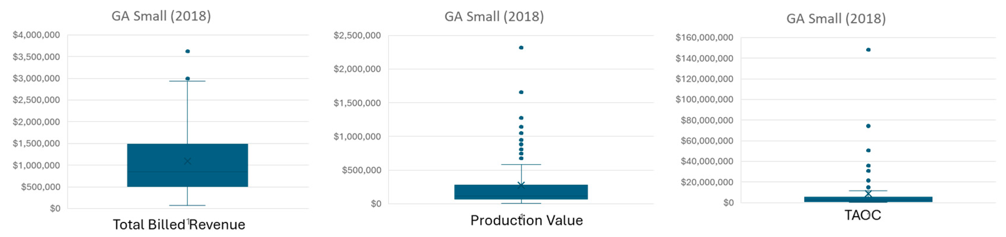
Supporting the analysis further and providing an additional graphical aide, box plots were developed for the data values shown in Figure 2. Box plots are used to visually summarize datasets, especially when comparing multiple groups, further assisting by helping to identify outliers, showing the spread of data, and showing distribution comparisons. Figure 3, Figure 4, Figure 5 and Figure 6 show the box plots, and Table 1 includes critical data from the tools used.

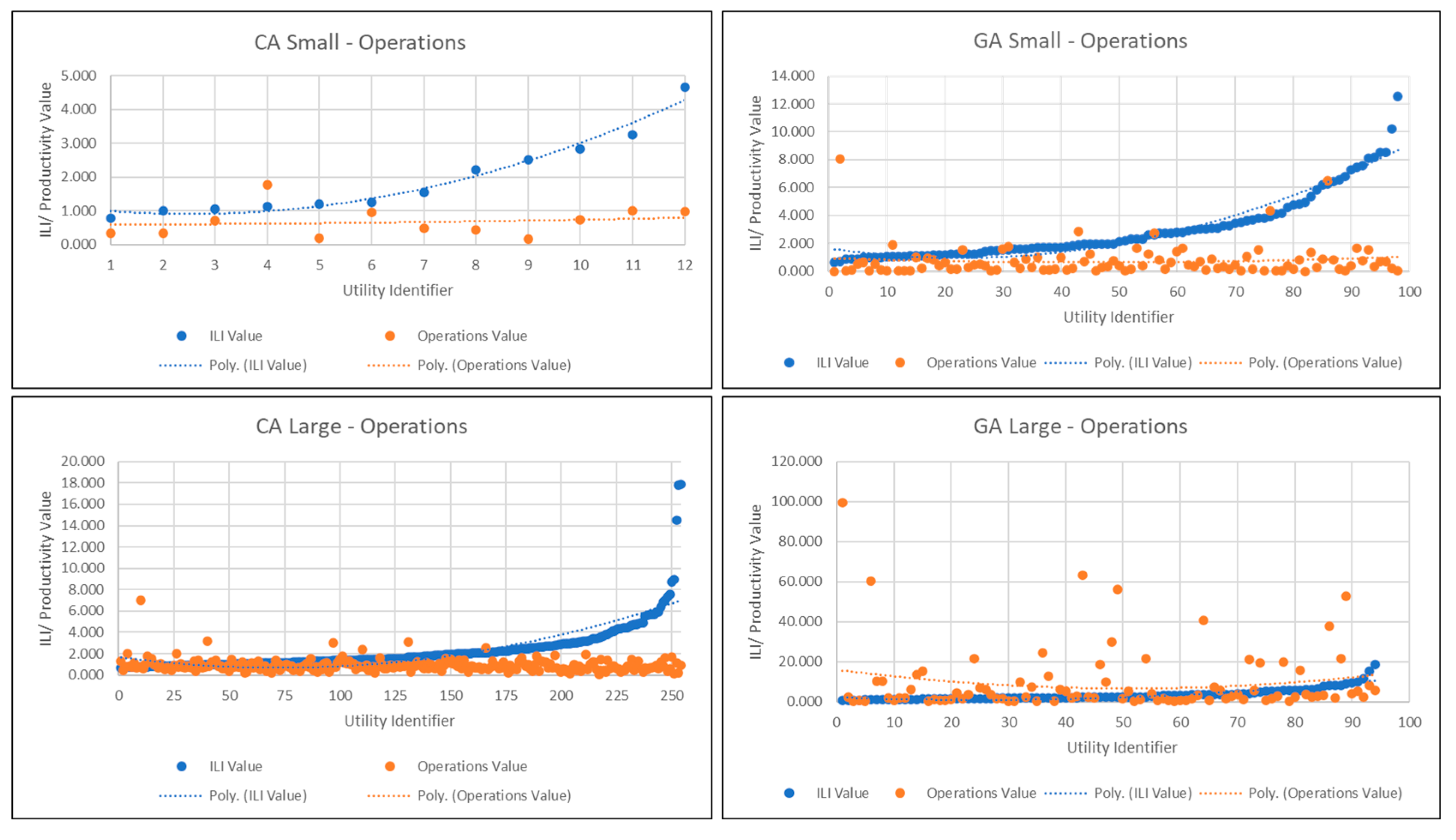
The next set of analyses (Figure 7 and Figure 8) graphically explored the Total and Partial Productivities of each utility versus their ILI within the different size and state groupings. It is interesting to note that, while, in general, ILI appears to increase non-linearly, there was overall a lack of a clear relationship between the population sizes and either of the productivity measures (at least within the size and state groupings). The aim of plotting this data was to observe any visual trends that may exist when water loss is compared to total operational productivity. A separate observation is within the CA Small grouping, where there is evidence of a U-shaped relationship between Partial Productivity and ILI (upper left quadrant of Figure 7); however, this grouping contains very few utilities (n = 12), and the same relationship is not visible amongst the other state-size groupings.

Although the 3-sigma data filter method of the Total Productivity values failed to have a significant impact on the data, further analysis, including unexpected observations in the data, appeared to show several datapoints out of family (i.e., the existence of outliers). It was posited that these might not have been identified by the 3-sigma method due to skewness in the data. Various filtering options were evaluated, and it was determined to apply the IQR statistical method to help identify and remove outliers amongst the dataset. The IQR method was selected as the methodology applied helps identifying outliers in skewed distributions and is less impacted by extreme data values, some of which were seen in the dataset. The 3-sigma method heavily relies on the mean and standard deviation which can be significantly impacted by outliers in non-normally distributed datasets. The IQR method is less susceptible to the influence of extreme values; the IQR method, thus, provides a more robust way to identify outliers compared to the 3-sigma method, which assumes a normal distribution.

The IQR statistical method was applied across all of the datasets. Post-filtering, data outliers were filtered on Total Productivity values from only the GA Small (5 points removed) and the CA Large (15 points removed) groupings:

• For CA Small—given the small sample size (n = 12) and less variation amongst the dataset, the calculated IQR value (0.61659) was small and suggested the central data are close together and, therefore, are more consistent, thus, no data points were removed;
• For GA Large—the calculated IQR value (8.07598) fell within the upper range of the dataset, thus, when performing the filter, no data points were removed.

In addition, specific to the CA Large data, two additional points were removed as cost data showed $0 USD or was not included for two of the utilities. Figure 9 displays the Total Productivity and Partial Productivity and their component metrics as similar to Figure 2, this time showing the results with the IQR Filter applied.

Similarly to what was performed prior to support Figure 2, box plots in Figure 10 and Figure 11 were added to aid the visual analysis of Figure 9, also with the IQR Filter applied. Only the CA Large and GA Small box plots are provided here as IQR filtering did not remove any additional observations from the CA small and GA large data (i.e., the CA Small and GA Large boxplots after IQR filtering are the same as those portrayed in Figure 3 and Figure 6, respectively).

As shown if Figure 12 and Figure 13, post-IQR filtering, the same graphical analyses captured in Figure 7 and Figure 8 were conducted again; however, no significant pattern change was observed in any of the graphical analyses after filtering was applied. The goal of the IQR filtering was to normalize the data for better comparison, specifically the GA Large data, as when evaluating Figure 2 and Figure 9, the GA Large (bottom right quadrant) is out of family when compared to the other groupings. In addition, after evaluating Figure 7 and Figure 8, the IQR filtering was also attempted to remove other outliers, which seem out of family as shown in the figures. However, Figure 12 and Figure 13, below, show a similar pattern to Figure 7 and Figure 8, respectively, even post-IQR filtering. Furthermore, as has been previously noted, interestingly, data points were removed based on the IQR filter only for CA Large and GA Small data, even though the GA Large data had originally been anticipated to potentially contain the most outliers. That is, even though the GA Large data shows unexpected and out of family behaviors, this does not seem to be due to the presence of formal outliers. As there was no change to the CA Small and GA Large datasets after the IQR filtering, the reader should refer back to Figure 7 and Figure 8 for the data for those groups.

Table 2. CA Large and GA Small Average Revenues and Cost Comparison with Standard Deviation and IQR values, post-IQR filtering.

Group	Standard Deviation	IQR Value
CA Large
Total Billed Revenue	$82,283,575	$20,341,665
Production Value	$13,099,244	$4,368,750
TAOC	$85,977,244	$23,833,396
GA Small
Total Billed Revenue	$746,898	$951,224
Production Value	$375,586	$201,774
TAOC	$23,588,842	$4,370,694

contains the updated values from Table 1 for the groupings where the IQR filter removed data points for CA Large and GA Small datasets. As noted before, there was no change to the CA Small and GA Large datasets after the IQR filtering, so the reader should refer back to Table 1 for the data for those groups.

Last, a two-sample parametric t-test (α = 0.05) was performed to compare the sample means of the two independent groups, comparing state-by-state grouping by size (small and large) as well as comparing the data within each state for Partial and Total Productivity measurements. This analysis was conducted with the post-filtered IQR data. (Note, it was determined not to include the GA Large data in the t-test due to previously noted issues with the data appearing to contain out of family observations and behaviors compared to the other data groupings, even after IQR filtering.) The results of the t-tests are shown below in

Table 3. CA (Small/Large) and GA (Small) Two Sample t-test Results.

Group	Result
CA vs. GA (Small) Two Sample t-test	P (T ≤ t) one-tail
Small—Operations/Total Productivity	0.165244
Small—Production/Partial Productivity	0.086991
CA (Small vs. Large) Two Sample t-test	P (T ≤ t) one-tail
CA—Operations/Total Productivity	0.173981
CA—Production/Partial Productivity	0.003936

. The test variable used in upper portion of Table 3 (“CA vs. GA (Small) Two Sample t-test”) is the state (Georgia and California) and two-tailed p-values are evaluated. The test variable used in the lower portion of Table 3 (“CA (Small vs. Large) Two Sample t-test”) is Size (CA—Small and CA—Large), and one-sided p-values are evaluated. Only one of the four analyses (CA—Production) found statistically significant differences across groups; specifically, Partial Productivity was lower in small utilities compared with large utilities. Thus, Hypothesis 1 is as expected only for the Partial Productivity metric in the state of CA.

A numerical correlation analysis was then conducted between ILI and the Productivity measures to directly explore the relationships between ILI and Productivity as graphically shown in Figure 7 and Figure 8, for Hypothesis 2 and Hypothesis 3, respectively. The results of the correlation analysis are shown below in

Table 4. CA and GA Numerical Correlation—ILI and Productivity Results.

Group	Correlation Value	P (T ≤ t) Two-Tail
CA Numerical Correlation
CA Small—Operations/Total Productivity	0.159976	0.619439
CA Small—Production/Partial Productivity	−0.183656	0.567753
CA Large—Operations/Total Productivity	−0.099412	0.114001
CA Large—Production/Partial Productivity	−0.043881	0.486278
GA Numerical Correlation
GA Small—Operations/Total Productivity	0.027409	0.788776
GA Small—Production/Partial Productivity	0.118099	0.246792

and no significant linear relationship (Hypothesis 2 and 3) was observed.

6. Discussion

Figure 2 and Figure 9 show significant variance among the groupings in terms of billed revenue compared to Operations and Production costs. The GA Large grouping appears to be incomplete or have errors in the data that was reported, when compared to the other three groupings, especially how the figure shows total billed revenue far exceeds both Operational and Production costs for the utility. That said, each of the quadrants (state-size groupings) shows Production costs lower than total Operations costs, which must logically be the case and, thus, if this pattern was not observed it might indicate issues in the researcher’s computation of Production costs or the utilities recording of the underlying cost and water supplied data.

From a top-level view, one could argue the utility passes on the costs of system inefficiency (water system losses) to the customer since no direct relationship is observed. In further review of the literature, most critical projects are generally funded through state grants or special projects funded by the federal government. One could claim the water utilities are compensating for water losses through consistent rate increases, but they are not reaching the root of the problem to address and mitigate the losses. From the AWWA dataset, Georgia state utilities billing rates per 1000 gallons [3785.41 L] rose on average 2.73% from 2016 to 2018, with additional increases since. In California, combined water and sewer bills increased by 4.1% per year on average, from 2012 to 2024 [38]. These extra costs through inefficiencies could be passed along to the customer by covering up the system inefficiencies without a direct plan on how to better manage the system and mitigate the losses to help keep rates steady. In addition, there really is no competition for an alternate water provider to keep the rates more competitive and push technical managers at the water utility to improve.

From Table 3, the low p-value in only one of the four groupings (below 0.05) indicates a statistically significant difference between groupings. This shows there is a relationship between the variables being studied in the population (CA Production/Partial Productivity). It is believed no relationship was established for the Small Operations and Productions set, due to the sample size for California being small (12 utilities) compared to the rest of the data groupings.

In evaluating the results of Table 4, three of the four correlation values in the upper portion of the table (“CA Numerical Correlation”) are negative, meaning one variable increases as the other decreases. This provides some support for Hypothesis 2 by implying an inverse relationship in three of the four groupings. The observed correlations are non-significant (i.e., cannot be convincingly shown to be different from zero). Thus, the overall conclusion is that Hypothesis 2 and Hypothesis 3 are NOT supported. The small sample size of the CA Small Total Productivity measurement is likely a primary reason for the discrepancy between this group’s results and those of other California groups. This is a positive story for the California utilities as for three of the four utility groupings, as production values increase, the water loss amounts tend to decrease.

The results of the lower portion of Table 4 (“GA Numerical Correlation”) shows Hypothesis 3 to be non-supported given both resulting values show positive correlation, meaning both variables tend to increase or decrease together. The observed correlations also appear to be non-significant. Based on these data, as Productivity increases at GA Small utilities, the amount of water lost due to leakage also increases.

Evaluating this further, more recent articles share the state of Georgia is raising rates across the state to support infrastructure maintenance and upgrades; this is a focused effort to address rising operational costs and infrastructure upgrades [39,40]. The rate increases in some counties will occur every other year up through 2031 [39].

The 2018 Georgia Water and Wastewater Rates Report states 48% of Georgia water utilities had their utility billing rate structures significantly changed across the state between 2017 and 2018 [41]. This could help explain why the Georgia Large data showed such a steep increase on Customer Bill Revenue when compared to utility costs, thus directly impacting the high productivity value. The report stated that the increases were mainly due to improved cost recovery efforts and higher monthly bills to the customer were a result [41]. The cost recovery effort aims to recoup some of the costs the utility from prior money spent on water processing and output production and also shared 25% of Georgia water utilities had not seen a rate increase since 2013 or prior, further justifying the cost recovery effort [41]. This rate increase could help address the need for infrastructure improvement related to increased water losses within the state.

Georgia and California have different approaches to water management, but both states face significant challenges in improving their water productivity and efficiency. In Georgia, the state’s water management plan focuses on increasing water supply and reducing demand, but it does not provide a comprehensive approach to improving water productivity and efficiency [32]. In California, the state’s water action plan emphasizes the importance of water efficiency and conservation [30], however the roadmap to execute is not clear.

7. Conclusions

This study provided a comparative examination of the infrastructure system operation and partial productivity of California and Georgia water utilities, with a focus on their relationship to population served and water loss. Examined include how utility size, governance, and financial resources impact overall performance, highlighting significant inefficiencies in water management systems. California and Georgia water utilities continue to face significant challenges in managing water losses and system inefficiencies. While both states have made efforts to address specific issues within the industry, gaps remain.

This research provides the water utility technical manager with an opportunity to better align customer billing with utility losses. From the data and in review of the literature, utilities must request additional project funding to directly support water loss improvement projects as the customer billing revenue, in most cases, supports normal projection costs and nothing more. Using standard productivity methodologies, a practical approach is demonstrated to evaluate water utility data, providing water utility managers with a new performance measurement tool to be used when comparing amongst utilities.

To improve water output productivity and efficiency in Georgia and California, both states should adopt a comprehensive approach that includes the following elements:

• Use of common Water Productivity Metrics: Develop and use water productivity metrics to measure and evaluate water output productivity, effectiveness, and efficiency; compare both within the state and outside of the state using AWWA performance guidance. Standardizing productivity measurements across water utilities could facilitate comparison and benchmarking, enabling more effective evaluations and improvements;
• Establish detailed sustainment plans for maintaining the water infrastructure system, to include proactive maintenance and funding structures to support improvement projects. This would fall into Operations costs or Total Productivity, which from the California analysis shows as this value increases, the water loss value decreases;
• Water utilities should consider opportunity cost in their investment decisions, as this can help optimize system performance and reduce total system costs;
• Consider alternative pricing structures, to promote water conservation and reduce costs; one option could be to establish tiered rate structures that charge customers higher rates for higher levels of water consumption and system loss. Improved rate structures would help offset costs for system improvements.

Georgia and California are both using the guidance of the AWWA in their water loss analyses; however, given some of the data uncertainties found in the analysis, a question could be asked if they are training their utility staff and auditors the same way. The consistency of applying the AWWA methods is critical to having useable water data for all states for collective knowledge and shared water loss improvement opportunities across all utilities. However, the potential ambiguity in the operations definitions provided by the AWWA and their interpretation by water utilities staff and auditors in using these methods could lead to incorrect results. The present methodology and approach, when applied correctly, can aid technical managers to evaluate the data to draw conclusions and implement improvement activities.

There is a relationship between water utility operation and production costs and system output and performance. However, the relationship is complex and per this study, influenced by the population served. This approach could be applied to other states as well; however, since many states are not using the AWWA Level 1 guidance, the results may be incomplete.

The results of this study show that system leakage can be a predictor of system performance. Opportunity cost is also an important consideration, as it can help utilities prioritize investments and optimize system performance. The findings provided herein emphasize the need for comprehensive and integrated approaches to water infrastructure system management, which consider the complex interactions between leakage, performance, and opportunity cost.

The limitations to this research include the following:

• Data reliability—after initial review, the GA Large data were removed from the full analysis as the data values appeared out of family when compared to the rest of the data groupings. This prevented a more in-depth analysis when comparing within and across state groupings;
• Total cost information—an attempt was made to evaluate total revenue to the utility, instead of solely evaluating customer billed revenue. While the analysis was still valuable to be able to compare to customer revenue, a more holistic approach in comparing total system performance could have been made with more available revenue data;
• Limited state data—the AWWA has only provided this analysis for Georgia and California from 2018 data, no recent updates have been made to include more recent data nor to include other states, due to the limitations of following the AWWA Level 1 Audit guidance.

The theoretical contribution of this research lies in its examination of the underlying relationships between key variables in water utilities, with a particular focus on ILI and facility size. By conceptualizing the water utility as a cost center, this study sheds light on the critical infrastructure connections between water loss and productivity. Furthermore, it explores the potential relationships between productivity and the two investigated variables, ILI and facility size, although the empirical evidence does not support a direct relationship. Notably, this research provides a logically sound argument for a potential linear relationship between productivity and ILI, which was the hypothesis tested in the study. However, the findings indicate that no such linear relationship exists, suggesting that non-linearity may be a plausible alternative explanation. The absence of empirical evidence supporting either a linear or non-linear relationship underscores the need for further investigation.

A potential next step could involve non-linear explorations of the relationships between these variables, which may reveal more complex patterns not captured through this research analysis. This could include examining the relationship between ILI and productivity using scatter plots or other visualization techniques to identify potential non-linear trends or interactions. A separate mathematical approach, Data Envelopment Analysis (DEA), a frontier analysis technique, could also be applied as a non-linear productivity metric to measure how efficient the utility managers are using its resources to evaluate system inputs and outputs. By pursuing this area of research, future studies can build upon the theoretical foundations established here and work towards a deeper understanding of the intricate relationships governing water utility operations.

Looking ahead to future research, by performing a more detailed Partial Productivity analysis, this research would focus on additional specific inputs (i.e., energy costs, water treatment costs) to develop a partial productivity measurement, then identify where the utility could improve performance in that area and decrease total costs. This could also include analysis of external factors impacting water utilities, including climate variability across the states and technology advancements not yet introduced to the industry. For example, the replacement of aged water meters with smart water meters and the introduction of advanced flow-modulated pressure control tools have been proven to help identify where system leakage exists and mitigate water main breaks. Angeospatial analysis (e.g., Moran’s I test) comparing the correlation amongst utilities of water loss and productivity in arid regions compared to humid regions may show differing water loss patterns by region. As CRUC varies widely across utilities, another evaluation that could be performed would be a comparison analysis of the ILI ratio metric to the individual water utility cost per gallon. This would be a deeper dive into how much the customer is paying per unit lost. Long-term infrastructure depreciation, regulatory compliance costs, and emergency response expenses could also be evaluated as total costs impacting future operational performance metrics. Additionally, a regression analysis could be performed to isolate the effects from additional operational factors and variables, including maintenance costs, aging infrastructure, administrative inefficiencies, and several other factors. Last, the Carl Vinson Institute of Government, Data Analytics Division at the University of Georgia is working on data collection with the Georgia Environmental Finance Authority (GEFA) to build a historical record for the Georgia Water Utility Rates. This activity aims to include utility water data, monthly billing metrics, and price increase analytics to help in further water utility performance analysis.