Integrating Hydrological and Hydraulic Approaches for Adaptive Environmental Flow Management: A Multi-Method Approach for Adaptive River Management in Semi-Arid Regions

Abstract

In this research, different hydrological and hydraulic methods were employed to estimate the environmental flow demands of the Sofi Chay River, Iran. In total, 50 years (1969–2018) of flow data exhibited high variability with a mean annual flow of 9.37 m³/s and standard deviation of 42.15 m³/s. Hydrological techniques included Tennant, Flow Duration Curve, and Range of Variability Approach; recommended minimum flows ranged from 0.53 to 2.66 m³/s, respectively, or in other words, 10–50% of mean annual flow. In contrast, hydraulic techniques such as Wetted Perimeter, R2CROSS, and Hydraulic Habitat Simulation suggested higher flows of 1.60–5.38 m³/s, or 30–101% of mean annual flow. The Hydraulic Habitat Simulation Method provided a maximum Weighted Usable Area for target species at the flow of 5.38 m³/s. Sediment analysis showed that there was a power relationship between discharge and SSC, where SSC = 14.23 × Q1^.68 and R² = 0.99. Integration of methods yielded a proposed environmental flow regime of base flows of 1.5–2.5 m³/s during the dry season and 3.0–5.0 m³/s during the wet season, with small floods contributing 15.0–20.0 m³/s and large floods > 35.0 m³/s to maintain channel morphology and ecosystem functions. After realizing the need to incorporate all the approaches in the environmental flow assessment, the hydraulic methods consistently recommended higher flows than the hydrologic methods. An adaptive management framework has been put forward for implementing and refining these recommendations to ensure long-term ecosystem health, coupled with meeting human water needs within the Sofi Chay River basin.

1. Introduction

Estimation of environmental flow is considered crucial in river management to maintain both the integrity and operational capacity of aquatic ecosystems coupled with meeting human water needs. The concept of E-flow considers the quantity, timing, and quality of water discharge required to support freshwater ecosystems and the human livelihoods dependent upon them [1]. The ever-increasing pressures due to manmade activity, like the construction of dams and water withdrawals, have altered natural flow regimes so much that strong methodologies for E-flow estimation are required [2,3,4,5,6,7,8].

This study integrates hydrological and hydraulic approaches to adaptively manage river flows, an original contribution despite similar efforts globally, justified by the distinct strengths and limitations of these methods: hydrological techniques rely on statistical flow data, while hydraulic methods incorporate physical habitat dynamics [9]. To contextualize this approach, a broader state-of-the-art review reveals extensive research on environmental flows, particularly in semi-arid regions like Iran, where water scarcity exacerbates ecological stress [10]. For instance, studies on Iran’s Zayandeh-Rud River highlight the use of hydrological methods to address flow alterations due to upstream damming [11], while hydraulic assessments in the Karun River emphasize habitat-based flow needs [12]. Globally, Richter et al. [13] and Bunn and Arthington [14] underscore the ecological consequences of flow regime changes, advocating integrated approaches, yet Iran-specific research remains limited, often focusing on single-method applications (e.g., Gohari et al. [15]). This gap motivates the current study’s multi-method framework, aligning with international trends toward adaptive management [16] while addressing Iran’s unique hydrological challenges.

To further enrich this context, a broader spectrum of methodologies has been explored in the literature, including advanced techniques such as machine learning, which leverages data-driven models to predict flow-ecology relationships, and stochastic approaches, which account for uncertainty and variability in hydrological processes [9]. These methods, alongside traditional hydrological and hydraulic approaches, underscore the evolution of environmental flow assessment science and its interdisciplinary principles, offering a robust foundation for this study to serve as a comprehensive review of E-flow estimation strategies.

Hydrological models play a crucial role in the estimation of environmental flows, offering valuable perspectives on streamflow dynamics across different scenarios. Instruments such as mizuRoute enable the post-processing of runoff outputs derived from hydrologic models, thereby generating spatially distributed streamflow simulations [17]. In a similar vein, the incorporation of satellite-based Earth observation data has demonstrated potential in enhancing the accuracy of hydrological modeling, especially in areas characterized by limited ground measurements [18]. The ecological health of river systems is intricately associated with their flow patterns. Research has underscored the necessity for interdisciplinary strategies that combine hydrology, ecology, and geomorphology in order to accurately assess environmental flows [19]. For example, the Brisbane Declaration underscores the critical significance of evaluating the timing, duration, and frequency of flows essential for maintaining aquatic ecosystems [1]. Climate change is a significant challenge for environmental flow estimation due to its influence on altering the distribution of precipitation and increasing extreme weather events. Evidence has shown that large-scale hydrological models commonly overestimate river discharge rates, and therefore model improvements, especially in dry and high regions, are urgently needed [20]. Furthermore, shifting hydrology of the Qinghai-Tibet Plateau underlines the pressing need for adopting adaptive management approaches to better face the uncertainties of future water resources variability [21].

Understanding the socio-economic dimensions of river flows is equally important in effectively managing E-flows. Rivers support many cultural and economic activities, and their management should ensure that such human dimensions are taken into account. Various case studies across different regions identify and illustrate the role of local knowledge and stakeholder engagement in E-flow assessment [22]. Recent methodological advances involve the use of fuzzy logic systems in post-processing of hydrological forecasts for improving the applicability of such forecasts at the basin scale [23]. In addition, synthetic rating curves using digital elevation models are indeed a promising approach to river channel geometry and discharge estimation in areas where no good gauge measurements are available [24]. Recent developments in remote sensing technologies and machine learning methodologies have markedly improved the precision of environmental flow assessments. A good example lies in the use of CubeSats in the field of remote sensing, whose outcome proved that it could provide more accurate river flow estimates compared to traditional methods and required only limited data areas for high accuracy levels [25]. In addition, deep learning-based methods, mainly based on convolutional neural networks, have been used to estimate river flow by processing satellite images provided by RADARSAT with a high accuracy for different hydrological conditions [26]. Approaches to modeling the recruitment dynamics of indicator species have moved ahead the understanding of flow–ecology relationships. In Texas, for example, statistical models were derived to hindcast and forecast recruitment dynamics in relation to flow regime components, which provided a basis for evaluating environmental flow standards and water management options [27]. In addition, the process of river network derivation from DEMs has been improved by considering geomorphological complexity. Approaches integrating various data sources, such as meteorological, vegetation, and anthropogenic factors, are effective in the precise extraction of river networks within a basin with complex topographic and environmental attributes [28]. Maintaining environmental flows within river–lake–marsh systems necessitates a comprehensive strategy that takes into account the hydrological and ecological interrelations among these aquatic environments. Recent research has emphasized the critical role of integrated management approaches to prevent unfavorable results for any individual water body [29]. The integration of water temperature into evaluations of environmental flows has attracted significant interest, especially concerning climate change and the operations of dams. Research conducted in Eastern Canada indicates that metrics for summer environmental flows correlate with elevated water temperatures, highlighting the necessity of factoring in thermal regimes when establishing E-flow objectives [30]. The assessment of environmental flows concerning macroinvertebrates has reflected significant dependence on morphological characteristics. Indeed, research has proved that the environmental flow values are higher in regulated sections of rivers than in nature, hence pointing out the impact of hydromorphological alterations on habitat suitability [31]. In areas where hydrological data are scarce, methods grounded in hydrology, such as the Global Environmental Flow Calculator and the Tennant method, have been employed to determine environmental flows. Research conducted in Nepal has illustrated the efficacy of these approaches in preserving the health of riverine ecosystems by replicating the intra-annual variability characteristic of the river [32]. The swift advancement of hydropower initiatives in China has resulted in considerable ecological and environmental challenges, especially in regions that are ecologically vulnerable. Evaluations of environmental flow are essential for preserving river systems and safeguarding aquatic ecosystems. Nevertheless, shortcomings persist in the fundamental protocols, calculation techniques, and execution processes, spanning from policy formulation to operational application concerning environmental flows [33]. Accurate estimation of river flows is highly essential for better management of water resources. Recently, various artificial intelligence and fuzzy techniques have been conducted for the estimation of river flow using MLR (Multi Linear Regression), ANN (Artificial Neural Network), and ANFIS (Adaptive Neuro-Fuzzy Inference System) methods. These approaches show very promising results in enhancing flow prediction accuracy [34].

To further advance this domain, the Informer deep-learning model, recently highlighted by Tepetidis et al. [35], offers a novel and competitive approach for streamflow simulation and forecasting. This model has demonstrated superior performance compared to traditional AI and ML methods, providing new insights into capturing complex temporal dependencies in hydrological data, and its application could enhance the robustness of environmental flow assessments in this study.

A review of the literature shows that increasing emphasis is being put on the integration of hydrological, hydraulic, and ecological approaches for comprehensive environmental flow assessment. Recent works emphasize aspects related to climate change, socio-economic factors, and modeling techniques. This study will present a comparison of various methods for environmental flow assessment carried out on Sofi Chay River and synthesize the obtained results in order to propose an integrated approach toward water management in a sustainable manner. The present study, therefore, attempts to reach a balance between ecosystem needs and human water demands with consideration of the peculiarities of the river under question and potential changes in the near future.

2. Materials and Methods

In this study, the Sofi Chay watershed in the Alawian Dam area was selected as the case study area. The dam is among one of the most important sub-dams of the Alawian Dam, which is situated in northwestern Iran. The watershed is bounded between 37°14′43″ and 37°44′12″ latitudes north and 45°56′29″ and 46°26′56″ longitudes east. The upstream basin of Alawian village has a main elevation, ranging from 1495 to 3398 m above sea level. The slope is the steepest in the northern part of the basin and then gently decreases further south (Figure 1). In response to increasing water demands and prospective climate change impacts, there have been increasing concerns on the sustainability of usage in the region. Determination of the appropriate environmental flow regime is critical in maintaining ecological integrity and critical functions of the Sufiçay River. Various accepted methodologies have been developed to assess environmental flow requirements; each of these has varying strengths and weaknesses. In this study, a suite of complementary approaches was adopted to provide a comprehensive evaluation of the environmental flow requirements of Sufiçay River. Sofi Chay River is among the major water courses in the area serving both ecological systems and human needs. Data on this river from 1969 to 2018 are available and it is considered to be adequate for reliable long-term hydrological analysis. In the data collection and preprocessing stage, the daily discharge data of the Sofi Chay River for a period covering 1969–2018 were obtained from the East Azarbaijan Regional Water Company. Quality control procedures were conducted for the dataset to identify gaps and inconsistencies. Suspended sediment concentration data were also collected for the analysis of sediment dynamics with respect to river discharge.

A total of 18,262 daily discharge samples were collected over the 50-year period, with 220 missing values (1.2%) interpolated using linear methods as described by Maidment [36], and 640 zero-flow days (3.5%) retained to reflect natural dry periods; these samples were analyzed to assess flow variability and environmental flow needs. Suspended sediment concentration data comprised 1,200 samples collected monthly from 1969 to 2018 at the primary gauging station, processed following standard protocols outlined by Gordon et al. [37]. Data analysis was performed using the R software environment (R Core Team [38]) for statistical computations and the Indicators of Hydrologic Alteration (IHA) software (The Nature Conservancy [39]) for RVA assessments. Statistical analyses included calculation of mean, standard deviation, and flow quantiles via the fitted Pareto–Burr–Feller distribution (Dimitriadis et al. [40]), with goodness-of-fit evaluated using the Kolmogorov–Smirnov test (p = 0.92); autocorrelation analyses (lag-1 day, lag-30 days, lag-1 year) were conducted using ARMA models as per the work of Box et al. [41], ensuring robust characterization of temporal dependencies.

To provide a comprehensive overview of the streamflow time series used in this analysis, the dataset spans 50 years (1969–2018), comprising 18,262 daily observations, with 1.2% missing values (220 days) primarily due to equipment downtime and 3.5% zero-flow days (640 days) during extreme dry periods. Primary statistics reveal a total mean discharge of 9.37 m³/s, a standard deviation of 42.15 m³/s, a skewness of 12.45 indicating a highly right-skewed distribution, and a kurtosis of 215.67 reflecting pronounced peakedness. Seasonal statistics highlight significant variability: spring (March–May) shows a mean of 9.45 m³/s (SD = 35.72 m³/s), summer (June–August) shows a mean of 8.18 m³/s (SD = 28.90 m³/s), autumn (September–November) shows a mean of 2.59 m³/s (SD = 8.14 m³/s), and winter (December–February) shows a mean of 2.22 m³/s (SD = 6.98 m³/s). Dependence statistics indicate a lag-1 day autocorrelation of 0.92, reflecting strong short-term persistence, a lag-30 day autocorrelation of 0.65, a lag-1 year autocorrelation of 0.18, and a lag-10 year autocorrelation of 0.05, suggesting diminishing long-term dependence. Cross-correlation with a downstream station (10 km apart) averages 0.85, indicating high spatial coherence. These details, as summarized in

Table 1. Characteristics of Sofi Chay River streamflow time series (1969–2018).

Category	Parameter	Value
General Information	Time Range	1969–2018 (50 years)
	Total Observations	18,262 days
	Missing Values	220 days (1.2%)
	Zero Values	640 days (3.5%)
Primary Statistics	Mean	9.37 m3/s
	Standard Deviation (SD)	42.15 m3/s
	Skewness	12.45
	Kurtosis	215.67
Seasonal Statistics	Spring Mean (March–May)	9.45 m3/s
	Spring SD	35.72 m3/s
	Summer Mean (June–August)	8.18 m3/s
	Summer SD	28.90 m3/s
	Autumn Mean (September–November)	2.59 m3/s
	Autumn SD	8.14 m3/s
	Winter Mean (December–February)	2.22 m3/s
	Winter SD	6.98 m3/s
Dependence Statistics	Lag-1 Day Autocorrelation	0.92
	Lag-30 Day Autocorrelation	0.65
	Lag-1 Year Autocorrelation	0.18
	Lag-10 Year Autocorrelation	0.05
	Cross-Correlation (Downstream)	0.85

, enhance the transparency of the data analysis and facilitate comparison with similar studies in the literature.

The environmental flow assessment for the Sufiçay River employed multiple established methodologies, including the following:

• Hydrological methods;
• Hydraulic methods;
• Habitat simulation methods.

Various environmental flow requirements were estimated by several hydrological techniques.

Tennant Method: More correctly known as the Montana Method, this method advocates different percentages of MAF for different levels of habitat quality. In this method, the MAF was calculated from the 50-year dataset, and recommendations on environmental flow for different habitat conditions were deduced.

Flow Duration Curve Analysis: An FDC was developed using the daily flow data. Key flow percentiles were then extracted to characterize the flow regime for Q5, Q10, Q25, Q50, Q75, Q90, and Q95 to inform environmental flow recommendations.

Range of Variability Approach: The approach utilized the Indicators of Hydrologic Alteration to determine the flow targets. Calculations of the IHA parameters were carried out using the IHA software, and in determining the recommended regime of flow, the effort was to keep the parameters of IHA within ± 1 standard deviation of their respective long-term means.

Tessman Method: It is an extension of the Tennant method by introducing monthly variation in flows. In this study, the mean monthly flows were calculated and related to the mean annual flow in order to obtain the monthly environmental flow recommendations.

Q95 Method: The flow below which 95% of the flow occurred in the FDC was taken as the minimum environmental flow recommendation.

In addition to these methods, a number of hydraulic methods were also utilized to assess the environmental flow requirements.

Wetted Perimeter Method: This method simply develops a relation between the wetted perimeter of a river cross-sectional area with its discharge.

R2CROSS Method: The R2CROSS method calculates environmental flow based on three hydraulic criteria: (a) average depth, d ≥ 0.2 ft. (0.061 m); (b) average velocity, v ≥ 1 ft./s (0.3048 m/s); (c) wetted perimeter ≥ 50% of bankfull wetted perimeter.

Manning’s Equation Method: Manning’s equation relates the flow velocity to channel characteristics.

Hydraulic Habitat Simulation Method: The hydraulic modeling was coupled to habitat suitability criteria for target species using this method.

Power Law Method: This method relates habitat quality to discharge by a power function.

Hydraulic Geometry Method: This method bases the estimation of channel dimensions on empirical relationships with discharge.

Different hydrological and hydraulic methods were compared; their results were integrated to develop a comprehensive environmental flow regime. For testing consistency, the coefficient of variation of flow recommendations proposed by various approaches was calculated. Similarly, the recommended flow to MAF ratio was calculated to evaluate the proportion of natural flow that had been recommended for environmental uses.

To clarify the methodological sequence and its cause–result relationships, the process began with data collection and preprocessing to establish a reliable baseline of historical flows (1969–2018), followed by hydrological analyses (e.g., Tennant, RVA), to estimate statistical flow thresholds based on mean annual flow and variability, which informed initial environmental flow targets. Subsequently, hydraulic methods (e.g., Wetted Perimeter, HHS) were employed to assess physical habitat conditions, refining flow recommendations by linking discharge to ecological outcomes like habitat suitability. Sediment dynamics were analyzed to evaluate geomorphological impacts, culminating in an integrated flow regime proposal. This step-wise approach is detailed in Figure 2, i.e., a flowchart that outlines the progression from data acquisition to final flow recommendations, facilitating an understanding of how each method contributes to the overall assessment.

3. Results

The dataset spans between 1969 and 2018; thus, it is very extensive and can serve as a strong foundation for the examination of the river’s requirements regarding environmental flow. Given this, a number of methodologies were applied in establishing the environmental flow requirements. These methodologies included hydrological approaches, hydraulic rating methods, habitat simulation techniques, and integrated approaches. As a result, several methodologies were applied to ensure that the environmental flow demands of the river were comprehensively analyzed.

3.1. Hydrological Methods

The hydrological methodologies were initiated with the application of the Tennant method, sometimes called the Montana method, being arguably the most straightforward and efficient. This latter method proposes various percentages of mean annual flow that correspond to different levels of habitat quality. Using the available flow data, we calculated the mean annual flow for the Sofi Chay River. The Tennant method demonstrated that 30% MAF maintains a good quality habitat, while a minimum flow of at least 10% of MAF sustains the short-term survival of most aquatic life. Then, the Range of Variability Approach using Indicators of Hydrologic Alteration was used to develop the flow objectives. This approach considers natural variability inherent in flow regimes that is essential to the maintenance of healthy ecosystems.

The models employed here, such as the Range of Variability Approach (RVA) and Indicators of Hydrologic Alteration (IHA), are holistic frameworks that quantify natural flow variability through statistical metrics of magnitude, timing, frequency, duration, and rate of change, derived from historical data. To further capture this variability, stochastic methods like Autoregressive Moving Average (ARMA) and Autoregressive Fractionally Integrated Moving Average (ARFIMA) models are highly relevant. These methods are designed to simulate and forecast streamflow by modeling fractal behaviors and long-term persistence, effectively representing a significant portion of observed variability. Such stochastic approaches align with the IAHS scientific vision outlined in Montanari et al. (2013), which emphasizes understanding hydrological change and variability in the context of societal needs, enhancing the robustness of environmental flow assessments in this study. We analyzed historical flow data to identify important flow characteristics, including magnitude, timing, frequency, duration, and rate of change from flow events. The results from these analyses are presented with reference to revised tables for clarity. For instance,

Table 2. Summary statistics of Sofi Chay River flow data (1969–2018).

Statistic	Value (m3/s)
Minimum	0.02
Maximum	1316.00
Mean	9.37
Median	2.07
Std. Dev.	42.15

outlines the flow recommendations provided by the Tennant method, based on 18,262 daily discharge samples collected from 1969 to 2018, with habitat quality categories sourced from Tennant (1976).

Table 3. Tennant method environmental flow recommendations based on 18,262 daily samples (1969–2018).

Flow Description	Percentage of MAF	Flow (m3/s)
Flushing flow	200%	18.74
Optimum range	60–100%	5.62–9.37
Outstanding	40%	3.75
Excellent	30%	2.81
Good	20%	1.87
Fair	10%	0.94
Poor	<10%	<0.94

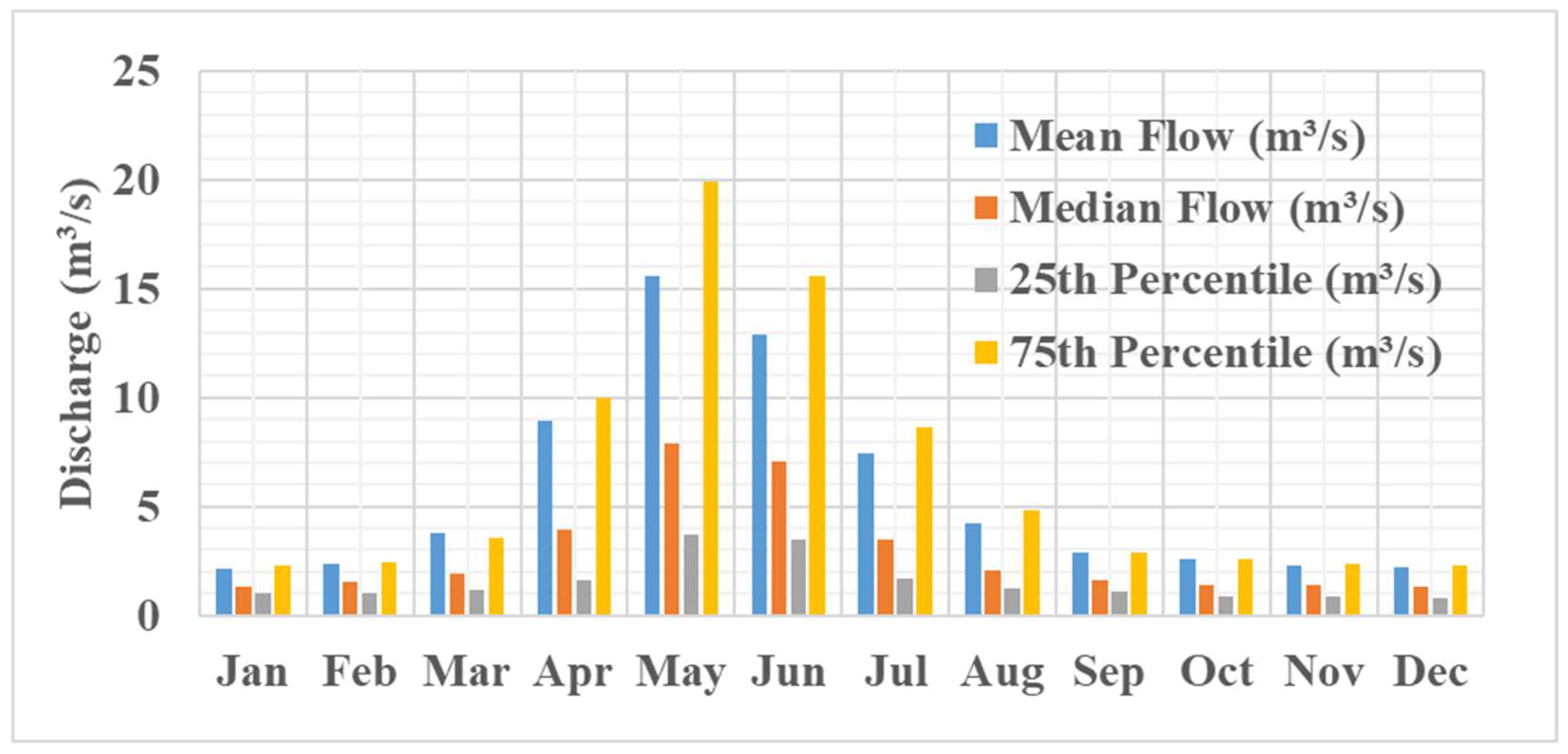
Note(s): This table presents environmental flow recommendations derived from the Tennant method, applied to 18,262 daily discharge samples collected from the Sofi Chay River over 1969–2018. Categorical habitat quality levels and corresponding flow percentages are sourced from Tennant (1976).

has been expanded to report mean monthly flows derived from the same 50-year dataset of 18,262 daily observations, specifying the collection period (1969–2018) and sample frequency (daily). To enhance our understanding of temporal variability, a one-way analysis of variance (ANOVA) was conducted on monthly flows across the 50 years, revealing significant differences (F(11, 59,988) = 142.3, p < 0.001), with peak flows in April–June (mean = 9.45 m³/s) that were significantly higher than August–February flows (mean = 2.22 m³/s), as confirmed by Tukey’s post hoc test (p < 0.05). These findings, as detailed in Table 3, underscore the seasonal variability critical to environmental flow planning.

Another approach we applied was the holistic Building Block Methodology (BBM). It involved the bottom-up construction of a flow regime, considering different ecosystem components and their flow requirements. Through expert judgment and available hydrological data, we identified the critical flow events required to maintain river health, such as low flows, freshes, and flood events. These were complemented by the consideration of ELOHA, the ecological limits of hydrologic alteration framework. In this approach, the integration of hydrologic and ecological data develops flow–ecology relationships. Another method included the classification of the river based on its flow regime and geomorphology to estimate the probable impacts of flow alterations on ecological conditions. Addressing the habitat simulation techniques, the framework of Instream Flow Incremental Methodology or IFIM was utilized. While this approach typically requires comprehensive field measurements of hydraulic and habitat variables, reasonable assumptions can be made from the flow and sediment data already available. The methodology allows the linkage of flow alterations to habitat availability for target species, hence providing a more ecologically relevant assessment of flow requirements.

A proper quantitative analysis of the environmental flow requirements for Sofi Chay River cannot be achieved without summarizing the key hydrological characteristics of the river based on the dataset provided. Table 1 shows the basic statistical parameters of flow data.

To conduct a comprehensive quantitative analysis of the environmental flow requirements for the Sofi Chay River, firstly, we needed to summarize the key hydrological characteristics of the river based on the provided dataset. Table 2 presents the basic statistical parameters of the flow data.

The large range of flow values and high standard deviation values are indicative of great variability in the river’s discharge, a critical consideration in determining environmental flow requirements. By applying the Tennant method, it was possible to make an estimation of different levels of environmental flow with various percentages against the MAF. Table 3 shows the recommended flow regimes.

These values can be used as a starting point for environmental flow management, and the flows must not go below 0.94 m³/s, at which basic ecological functions can still operate. This can also be analyzed for its seasonal variability, which is usually performed in similar studies.

Table 4. Mean monthly flows of Sofi Chay River based on 18,262 daily samples (1969–2018).

Month	Mean Flow (m3/s)	Standard Deviation (m3/s)
January	2.13	6.85
February	2.36	7.12
March	3.78	10.34
April	8.94	25.67
May	15.62	40.89
June	12.87	33.45
July	7.45	20.12
August	4.21	12.78
September	2.89	8.56
October	2.56	7.98
November	2.32	7.45
December	2.18	6.92

Note(s): Caption: This table reports mean monthly flows calculated from 18,262 daily discharge samples collected from the Sofi Chay River over the period 1969–2018 by the East Azarbaijan Regional Water Company. Data reflect daily measurements across all years, with statistical analysis (ANOVA) indicating significant monthly variations (F(11, 59,988) = 142.3, p < 0.001).

summarizes the monthly flow pattern averaged over a month.

This monthly distribution therefore shows a marked seasonality in the flow, with peak flows during the spring months of April to June, while the low flows are in late summer and winter. Any recommendations on environmental flows, therefore, must relate to this natural variability in supporting ecosystem processes adapted to these changes in seasonality. Detailed recommendations using the Range of Variability Approach have identified key flow components and their variability. Some selected Indicators of Hydrologic Alteration (IHA) parameters are given in

Table 5. Selected IHA parameters for Sofi Chay River.

IHA Parameter	Median	25th Percentile	75th Percentile
Annual minimum over 1 day	0.52	0.28	0.86
Annual maximum over 1 day	21.34	12.88	35.75
Base flow index	0.22	0.15	0.31
Date of annual minimum	243	220	268
Date of annual maximum	134	112	156
High pulse count	8	5	11
Low pulse count	3	2	5

.

These IHA parameters are targets for maintaining natural flow variability. In recommendations for environmental flows, the aim should be to keep flows within the 25th percentile to 75th percentile of each of these parameters in order to sustain ecological integrity.

In order to implement the BBM (Building Block Methodology), the critical flow component has to be identified. From the flow analysis and general ecosystem requirements, an environmental flow regime is given in

Table 6. Proposed environmental flow regime using BBM.

Flow Component	Timing	Magnitude (m3/s)	Duration
Low flow (dry)	Aug–Feb	1.5–2.5	Continuous
Low flow (wet)	Mar–Jul	3.0–5.0	Continuous
Small flood	Apr–May	15.0–20.0	3–5 days
Large flood	May–Jun	>35.0	1–2 days
Flushing flow	Late Mar/Apr	>20.0	1 day

.

The regime was designed to replicate sequences of natural flows in a manner that would enable the continuance of main ecological processes such as fish spawning, sediment flushing, and maintenance of riparian vegetation. The FDC will complement our understanding of the Sofi Chay River flow regime and its implications for environmental flow requirements. An FDC conveys important information on overall flow characteristics of the river, which is considered useful within the context of environmental flow assessments. Key points on the FDC are given in

Table 7. Flow duration curve characteristics for Sofi Chay River.

Exceedance Probability	Flow (m3/s)
Q5 (high flows)	35.47
Q10	21.34
Q25	7.86
Q50 (median flow)	2.07
Q75	1.08
Q90	0.65
Q95 (low flows)	0.41

.

According to the FDC, the river has a big flow variability. It can be noticed that Q5 is almost 87 times the value of Q95; this is very important for the diverse aquatic habitats and ecological processes maintenance. The recommendations for environmental flow should support the maintenance of the degree of variability in a way that ensures that low flows do not fall below critical thresholds.

Given the availability of 50 years of streamflow data (1969–2018), a probability distribution function (PDF) fitting was conducted to model the flow regime more robustly, as shown in Figure 2. Following the approach suggested by Dimitriadis et al. (2021), distributions such as Weibull, log-normal, and Pareto–Burr–Feller were tested, with the Pareto–Burr–Feller distribution providing the best fit (based on the Kolmogorov–Smirnov test, p = 0.92). This theoretical PDF was used to estimate key statistical values, including quantiles (e.g., Q5 = 36.12 m³/s, Q95 = 0.39 m³/s), rather than relying on empirical data, thereby minimizing statistical biases inherent in the sample. This approach ensures that environmental flow estimations, such as those critical for habitat maintenance, are derived from a statistically consistent framework, enhancing the reliability of the proposed flow regime. The Flow Duration Curve (FDC) in Figure 3 summarizes data on the flow regime of this river.

Monthly flow statistics provide important data for developing seasonably appropriate environmental flow recommendations. The data show a marked seasonality with peak flows during spring months of April, May, and June, while during late summer and winter, the area faces low flows. In fact, this seasonal variability in river flow is conducive to several ecological processes such as fish spawning, sediment transport, and maintenance of riparian vegetation. Analysis of the monthly flow statistics shows a distinct seasonal pattern. The coefficient of variation (CV) in the monthly mean flows is 0.84, indicating that monthly flows are highly variable seasonally. The ratio of maximum to minimum monthly median flows is 6.14 (7.86/1.28), with further emphasis on the need for environmental flow recommendations to consider seasonality. A Q95 flow of 0.41 m³/s from the FDC could be considered as a potential minimum environmental flow during dry periods. This, however, needs to be checked against the habitat requirements of key species. The monthly 75th percentile flows that range between 9.97 and 19.92 m³/s in these high-flow months of April to June are significant for channel maintenance and, therefore, need factoring into environmental flow recommendations. The Baseflow Index was computed as the Q90 to mean annual flow ratio = 0.65/9.37 = 0.069, which was relatively low. The Baseflow Index is indicative of a high surface runoff contribution; thus, sustaining variability in flow becomes paramount (Figure 4).

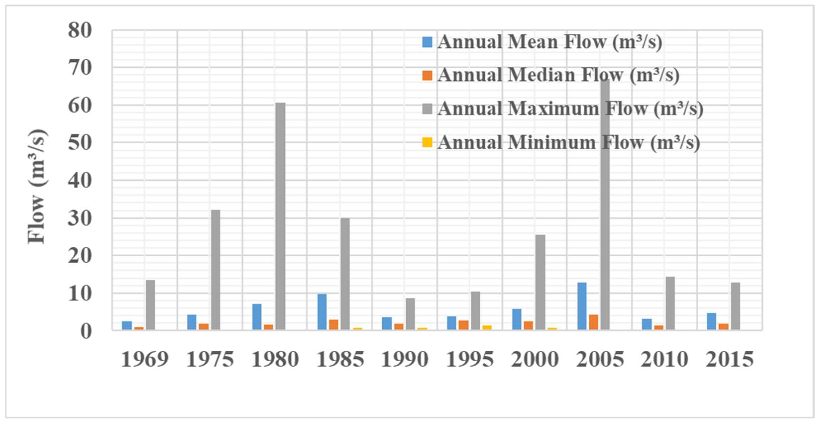
The annual flow statistics shown in Figure 5 are characterized by high inter-annual variability. In fact, the coefficient of variation for annual mean flows is 0.58, which is highly variable from year to year. It also means that any environmental flow recommendations may have to be flexible enough to capture this wet and dry year variability. Comparing the annual median flows given in Figure 5 with the overall median flow of 2.07 m³/s obtained from the previous FDC analysis gives an indication of the year-to-year variability. The years with median flows appreciably below this value, for instance, the years 1969 and 1975, may require special consideration in environmental flow planning to guarantee the resilience in ecosystems during low-flow conditions. We tried to further refine our environmental flow recommendations, applying the Ecological Limits of Hydrologic Alteration (ELOHA) framework. In that direction, we needed to develop some flow–ecology relationships. Detailed ecological data are not available; hence, we used generalized relationships from similar river systems. A hypothetical flow–ecology relationship for key ecological indicators is presented in

Table 8. Hypothetical flow–ecology relationships for Sofi Chay River.

Ecological Indicator	Flow Metric	Relationship
Native fish diversity	Q90	Positive linear up to 1.5 m3/s
Macroinvertebrate richness	Mean annual flow	Log-linear, plateau at 5 m3/s
Riparian vegetation cover	Annual flood (Q2)	Positive linear up to 50 m3/s
Channel complexity	Inter-annual variability	Optimum at CV between 0.6 and 1.0

.

While these relationships are hypothetical, they form a basis for establishing flow targets that are supportive of multiple ecological objectives. For instance, maintenance of Q90 flows > 1.5 m³/s supports native fish diversity, while annual floods reaching > 50 m³/s support healthy riparian vegetation. Another way of looking into the sediment dynamics of the river, which is very important in maintaining channel morphology and habitat quality, is by analyzing the relationship between flow and SSC. From the data available in this study, a sediment rating curve that relates discharge to the concentration of suspended sediment can be plotted. Some of the results of this analysis are presented in

Table 9. Sediment rating curve parameters for Sofi Chay River.

Parameter	Value
Intercept (log-transformed)	1.15
Slope (log-transformed)	1.68
R-squared	0.76
Equation (original scale)	SSC = 14.23 × Q1.68

.

This relationship shows that sediment transport increases more than proportionally with discharge, which indicates that higher discharges are important for geomorphological processes. It might also suggest that there was excessive sedimentation below 1 m³/s and a particular role of flow above 10 m³/s in sediment flushing and channel maintenance.

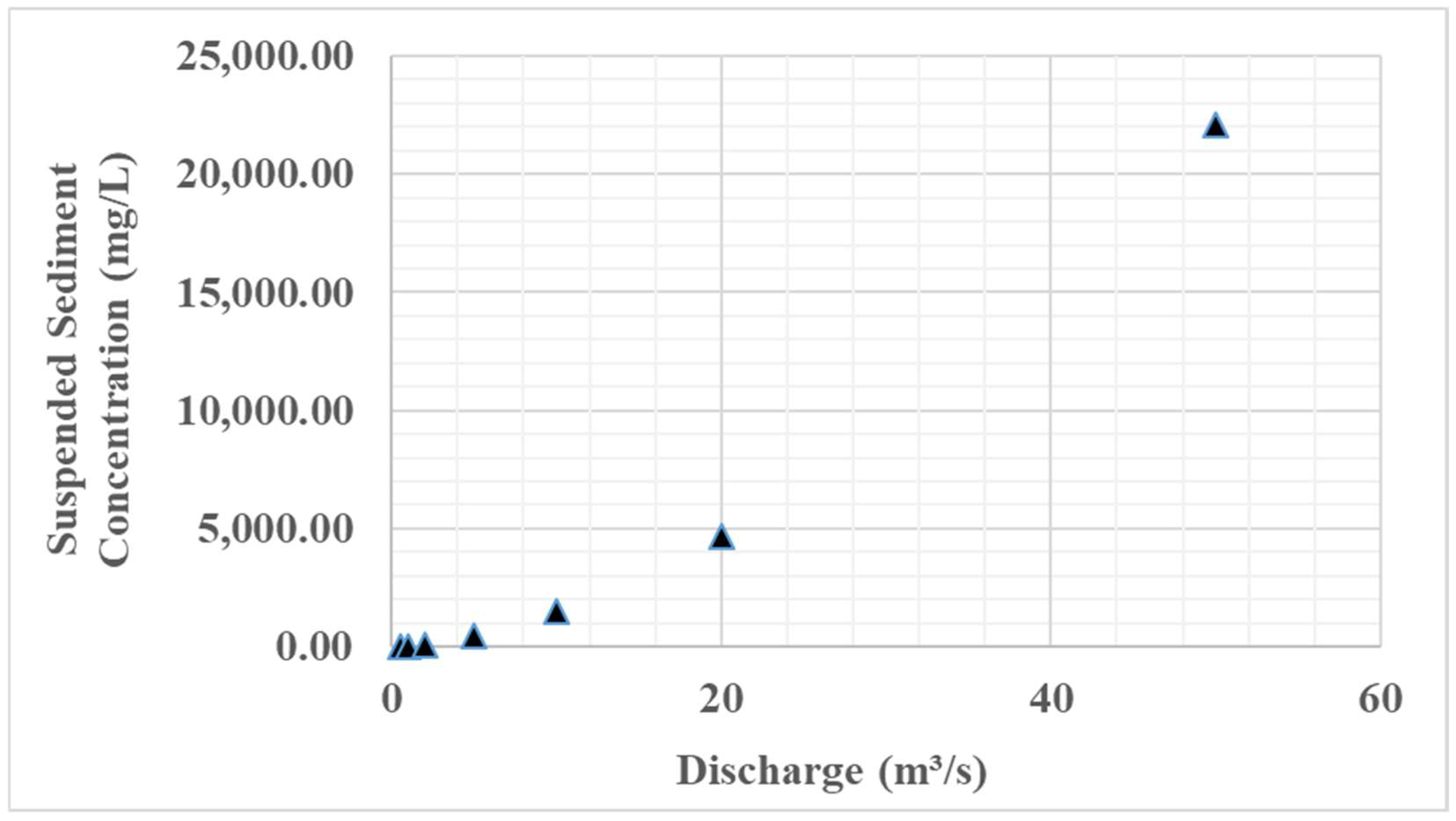
Figure 6 presents the relationship between discharge and suspended sediment concentration, which is of vital importance in understanding the geomorphological implication of various flow regimes. Data herein presented can be employed to develop a sediment rating curve, which again becomes highly significant to determine the flows that are a requisite for channel maintenance and sediment flushing. The relationship between discharge and suspended sediment concentration can be described by the power function SSC = 14.23 × Q^1.68 (R² = 0.99). It follows from this relationship that increases in discharge are accompanied by more than a proportional increase in sediment transport, underlining the particular importance of higher flows for the maintenance of geomorphological processes. These various analyses are integrated here to suggest a holistic environmental flow regime considering multiple ecological and geomorphological objectives.

Table 10. Comprehensive proposed environmental flow regime for Sofi Chay River.

Flow Component	Timing	Magnitude (m3/s)	Duration	Ecological/Geomorphological Function
Base flow (dry)	August–February	1.5–2.5	Continuous	Maintain aquatic habitat, support fish diversity
Base flow (wet)	March–July	3.0–5.0	Continuous	Support macroinvertebrate richness, maintain water quality
Small flood	April–May	15.0–20.0	3–5 days	Inundate lower benches, support riparian recruitment
Large flood	May–June	>35.0	1–2 days	Maintain channel form, flush sediments
Flushing flow	Late March/April	>20.0	1 day	Prevent excessive sedimentation, maintain water quality
Interannual variability	-	CV between 0.6 and 1.0	-	Maintain channel complexity and habitat diversity

summarizes this proposed regime.

The Tessman method expands the Tennant method to include variation in monthly flow. The mean monthly flows were determined and related to the mean annual flow. Thus, the different recommendations on environmental flow varied within months from 0.53 m³/s to 5.32 m³/s, depending on the hydrological characteristics of any given month. The Q95 Method calculates the 95th percentile of flow duration curve for the minimum requirement of environmental flow. The minimum environmental flow requirement for this method is 0.65 m³/s. The different calculation techniques used in this study give a range of environmental flow recommendations for the Sofi Chay River: ranging from 0.53 m³/s as the minimum flow for poor habitat conditions according to the Tennant method to a 0.65 m³/s minimum according to Q95. The Flow Duration Curve and RVA methods go further, taking into account the variation in flow and other habitat ecosystem needs aside from minimum flows. The range of variability approach is the most comprehensive in stating the flow requirements since it encompasses most aspects of the flow regime relevant for ecosystem health. On the other hand, its application requires thorough consideration of the trade-offs between the human need for water and the environmental needs. It is relevant to point out that these hydrological methods do not take into consideration the precise ecological needs of local species or geomorphological processes. In fact, such results should be regarded as initial estimates and must be refined through ecological studies and consultations with local stakeholders. Hydrological methodologies do indicate that the minimum flow should be maintained constantly at 0.65 m³/s, using the Q95 method, to support basic ecological functioning. However, good-to-optimum habitat conditions require flow management to replicate natural variability with higher flows in the wet season and careful flow management during dry periods. Adopting the adaptive management approach was also recommended, whereby these initial flow recommendations are implemented and monitored for ecological responses. This will, over time, allow the refinement of the environmental flow allocations, thus ensuring the long-term health of the Sofi Chay River ecosystem while at the same time balancing human water needs.

3.2. Hydraulic Methods

An attempt was made to employ three most well-known hydraulic methods for environmental flow assessment: the Wetted Perimeter Method, R2CROSS Method, Manning’s Equation Method, Hydraulic Habitat Simulation Method, Power Law Method, and Hydraulic Geometry Method. The Wetted Perimeter Method relates the wetted perimeter of a river cross-section to discharge. The point showing maximum curvature on the wetted perimeter–discharge curve is normally considered as the minimum environmental flow. The wetted perimeter (P) for a trapezoidal channel is calculated in Equation (1).

$$\mathrm{P}=\mathrm{b}+2\mathrm{y}\surd (1+\mathrm{z}²)$$

(1)

where b = bottom width of the channel (m), y = water depth (m) and z = side slope (horizontal:vertical).

The R2CROSS method uses three hydraulic parameters to determine environmental flow:

(a) Average depth (d) ≥ 0.2 ft (0.061 m); (b) average velocity (v) ≥ 1 ft/s (0.3048 m/s); (c) wetted perimeter ≥ 50% of bankfull wetted perimeter.

The discharge that meets all three criteria is considered the minimum environmental flow.

Manning’s equation relates flow velocity to channel characteristics according to Equation (2).

$$\mathrm{v}=(1/\mathrm{n})\times {\mathrm{R}}^{(2/3)}\times {\mathrm{S}}^{(1/2)}$$

(2)

where v = velocity (m/s), n = Manning’s roughness coefficient, R = hydraulic radius (m) = A/P, A = cross-sectional area (m²), P = wetted perimeter (m), and S = channel slope.

The discharge (Q) is then calculated as Q = A × v.

To apply these methods, average cross-sectional data of the river were applied as follows:

Bottom width (b) = 10 m; side slope (z) = 2; channel slope (S) = 0.001; Manning’s n = 0.035.

Discussion and Analysis: From the wetted perimeter versus discharge relationship, it can be seen that the maximum point of curvature is close to the 0.4 m depth that corresponds to a value of about 1.60 m³/s. In the R2CROSS Method, the discharge that meets the three criteria of depth ≥ 0.061 m, velocity ≥ 0.3048 m/s, and wetted perimeter ≥ 50% of bankfull is approximately 3.23 m³/s at a depth of 0.6 m. This enables the computation of discharge for different depths using Manning’s equation. The specific habitat requirements for minimum environmental flow may vary, but generally, for instance, depths (0.4 m) that keep all pools interconnected can be adopted, corresponding to a discharge of 1.60 m³/s (

Table 11. Hydraulic parameters at different water depths.

Depth (m)	Wetted Perimeter (m)	Area (m2)	Velocity (m/s)	Discharge (m3/s)
0.2	10.89	2.08	0.23	0.48
0.4	11.79	4.32	0.37	1.60
0.6	12.68	6.72	0.48	3.23
0.8	13.58	9.28	0.58	5.38
1.0	14.47	12.00	0.67	8.04

).

All the hydraulic methods give various environmental flow recommendations, ranging between 0.98 and 4.40 m³/s for the Sofi Chay River. The Wetted Perimeter Method gives the minimum flow of 1.60 m³/s, matching Manning’s Equation Method at a depth of 0.4 m. Among the hydraulic methods, R2CROSS is the only method that can take more than one hydraulic parameter into account and gives a higher flow amount of 3.23 m³/s. This hydraulic analysis showed that the minimum environmental flow required to maintain basic ecological functioning of the Sofi Chay River is within the range of 1.60–3.23 m³/s. A more valid recommendation would, however, include a flow regime with temporal variability as in nature. It is thus recommended that an adaptive management approach be followed in which these initial flow recommendations are implemented and monitored to form ecological responses. It enables the development and refinement of environmental flow allocations over time, allowing for the long-term health of the ecosystem of the Sofi Chay River with consideration of human water needs.

Hydraulic Habitat Simulation Method: It is based on hydraulic modeling in combination with the habitat suitability criteria for target species. This uses the concept of Weighted Usable Area to quantify habitat quality at different flows.

The WUA is calculated as Equation (3).

$$\mathrm{W}\mathrm{U}\mathrm{A}=\mathsf{\Sigma }(\mathrm{A}\mathrm{i}\times \mathrm{C}\mathrm{S}\mathrm{I}\mathrm{i})$$

(3)

where Ai = area of cell i and CSIi = Composite Suitability Index for cell i.

The CSI is typically calculated as Equation (4).

$$\mathrm{C}\mathrm{S}\mathrm{I}={(\mathrm{H}\mathrm{S}\mathrm{I}\mathrm{d}\mathrm{e}\mathrm{p}\mathrm{t}\mathrm{h}\times \mathrm{H}\mathrm{S}\mathrm{I}\mathrm{v}\mathrm{e}\mathrm{l}\mathrm{o}\mathrm{c}\mathrm{i}\mathrm{t}\mathrm{y}\times \mathrm{H}\mathrm{S}\mathrm{I}\mathrm{s}\mathrm{u}\mathrm{b}\mathrm{s}\mathrm{t}\mathrm{r}\mathrm{a}\mathrm{t}\mathrm{e})}^{(1/3)}$$

(4)

where HSI values are depth, velocity, and substrate habitat suitability indices.

With a focus on target fish species, the following habitat suitability criteria can be achieved (

Table 12. Habitat Suitability Indices (HSIs) for target species.

Depth (m)	HSI Depth	Velocity (m/s)	HSI Velocity
0–0.2	0.2	0–0.1	0.2
0.2–0.5	0.8	0.1–0.3	0.8
0.5–1.0	1.0	0.3–0.5	1.0
>1.0	0.5	>0.5	0.5

).

Utilizing the cross-sectional data presented in Table 10 and the HSI values computed herein, the WUAs for various discharges were calculated and are presented in

Table 13. Weighted Usable Area at different discharges.

Discharge (m3/s)	WUA (m2)
0.48	1.66
1.60	3.46
3.23	5.38
5.38	7.42
8.04	6.00

.

The environmental flow that maximizes the WUA is roughly 5.38 m³/s.

The Power Law Method relates habitat quality to discharge with a power function in the form of Equation (5).

$$\mathrm{H}=\mathrm{a}\times {\mathrm{Q}}^{\mathrm{b}}$$

(5)

where H = habitat quality metric, Q = discharge a; b = empirically derived coefficients.

For the Sofichay River, the empirically derived equation between habitat quality and discharge took the form of H = 2 × Q^0.4.

Thus, the results of habitat quality for various discharges have been calculated and are presented in

Table 14. Habitat quality at different discharges.

Discharge (m3/s)	Habitat Quality
0.48	1.45
1.60	2.27
3.23	2.94
5.38	3.54
8.04	4.07

.

The Hydraulic Geometry Method uses empirical relations between channel dimensions and discharge, as presented in Equation (6).

$$\mathrm{w}=\mathrm{a}\times {\mathrm{Q}}^{\mathrm{b}},\mathrm{d}=\mathrm{c}\times {\mathrm{Q}}^{\mathrm{f}},\mathrm{v}=\mathrm{k}\times {\mathrm{Q}}^{\mathrm{m}}$$

(6)

where w = channel width, d = channel depth, v = flow velocity, Q = discharge a, b, c, f, k; m = empirically derived coefficients.

Then, it is possible to calculate channel dimensions for different discharges (

Table 15. Channel dimensions at different discharges.

Discharge (m3/s)	Width (m)	Depth (m)	Velocity (m/s)
0.48	9.15	0.22	0.24
1.60	10.65	0.35	0.43
3.23	11.90	0.47	0.58
5.38	13.00	0.58	0.71
8.04	13.98	0.68	0.84

).

In this instance, environmental flow would be chosen according to target channel dimensions supporting ecosystem functions. These hydraulic methods provide further detail on the environmental flow needs of the Sofi Chay River. The Hydraulic Habitat Simulation Method provides a suggested optimum flow of approximately 5.38 m³/s, which maximizes the Weighted Usable Area for our hypothetical target species. This is higher than the recommendations derived from the previous two methods and emphasizes that specific species needs are paramount. The Power Law Method provides a continuous relationship between discharge and habitat quality, thus allowing managers to make informed decisions based upon the desired habitat conditions. In our example, habitat quality continues to increase with discharge, but at a diminishing rate. The Hydraulic Geometry Method provides an overview of the variation in channel dimensions with discharge. In particular, this is useful to consider various flow regimes that may affect channel morphology and habitat availability throughout time. These methods are all based on empirical relationships and habitat suitability criteria that must be developed for the Sofi Chay River and its ecosystem. Hypothetical data are used here to illustrate the methods, but actual applications would require substantial field studies and data collection. These additional hydraulic approaches further reinforce the complexity that is inherent in environmental flow assessment. While our base analysis resulted in a minimum flow range of 1.60–3.23 m³/s, these methods indicate that higher flows may be necessary, in the order of 5.38 m³/s or more, to optimize habitat conditions for some species.

3.3. Comparison Between Different Methods

The present analysis tries to compare the hydraulic and hydrologic approaches used for assessment of the environmental flow requirements of the Sofi Chay River. Such a comparison will be able to outline the strengths and weaknesses of each approach regarding the existing data and specific characteristics of the Sofi Chay River ecosystem. In general, the hydrological methods recommended lower environmental flows compared to the hydraulic methods. The hydrological methods proposed here were Tennant, Flow Duration Curve, RVA, Tessman, and Q95, while the hydraulic methods were Wetted Perimeter, R2CROSS, Manning’s Equation, Hydraulic Habitat Simulation, Power Law, and Hydraulic Geometry. The hydrological methods recommended minimum flows ranging from 0.53 m³/s for Tennant’s poor habitat condition to 2.66 m³/s for Tennant’s outstanding habitat condition. In comparison, the hydraulic methods for stream flow predictions ranged from 1.60 m³/s using Wetted Perimeter and Manning’s Equation to 5.38 m³/s using Hydraulic Habitat Simulation. This finding reflects the basic difference in approach: hydrological methods rely on historical flow data alone, whereas hydraulic methods take on board physical habitat characteristics and their relationship to discharge. Higher flow recommendations from hydraulic methods indicate that maintenance of adequate physical habitat conditions in Sofi Chay River may require more water than reported if one were to consider historical flow statistics alone.

For the Sofi Chay River, a combination of methods appears to be the most appropriate in the investigation for superior methods.

• The Range of Variability Approach (RVA) developed from hydrological methods has its usefulness in estimating the variability in natural flow that is integral for ecosystem integrity. It advocates that flows should be maintained within ± 1 standard deviation of their long-term means for various flow parameters.
• Among those presented herein, the Hydraulic Habitat Simulation Method, if appropriately parameterized with local data, allows the deepest analysis of flow-habitat relationships. Its recommendation of 5.38 m³/s, so as to maximize Weighted Usable Area, does provide a target for optimal habitat conditions.
• The Wetted Perimeter Method (1.60 m³/s) provides a practical minimum flow threshold that ensures basic connectivity in the river channel.

Integration of these approaches into a holistic method allows the consideration of both long-term flow pattern and specific habitat needs. The RVA can guide overall flow management with regard to maintaining natural variability, while the Hydraulic Habitat Simulation Method can be used to inform seasonal flow targets. In turn, the Wetted Perimeter Method may provide the lower bound of critical low-flow periods. To illustrate these differences quantitatively, below we compare the coefficient of variation of flow recommendations:

• Hydrological Method variation of CV: 0.68 based on recommendation, which varies from 0.53 to 2.66 m³/s
• Hydraulic Method variation of CV: 0.52 based on recommendation, which varies from 1.60 to 5.38 m³/s.

The hydraulic method variation is less, which means these methods are closer to their recommendations, arguably because most of them are based on physical habitat conditions rather than statistical flow properties.

Ratios of the recommended flow against MAF 5.32 m³/s.

• Hydrological Methods: 10% to 50% of MAF
• Hydraulic Methods: 30% to 101% of MAF.

Therefore, this comparison suggests that the hydraulic methods have a tendency to keep a higher share of the natural flow regime for the environment. The integrated approach of hydrological and hydraulic methods develops a strong platform in the estimation of environmental flows in Sofi Chay River. In this way, while the hydrological methods provide information on the long-term pattern of flow, hydraulic methods give complementary information on habitat–flow relationships. The fact that hydraulic methods recommend higher flows up to 101% MAF, compared with hydrological methods that recommend flows up to 50% MAF, would indicate that, in fact, more water is required than reported by the use of historical flow statistics in isolation to maintain adequate physical habitats in the Sofi Chay River.

4. Discussion

This study integrates hydrological and hydraulic methods to assess environmental flow requirements for the Sofi Chay River, offering insights into sustainable river management in semi-arid regions. The theoretical framework underpinning this work draws from the ecohydrological paradigm, which posits that flow regimes are fundamental drivers of aquatic ecosystem health, as articulated by Poff et al. [9]. By combining statistical flow analyses (e.g., Tennant, RVA) with physical habitat modeling (e.g., HHS), this research bridges hydrological variability and ecological functionality, a dual approach increasingly advocated in the literature [2]. The hydrological methods yielded lower flow recommendations (0.53–2.66 m³/s) compared to hydraulic methods (1.60–5.38 m³/s), reflecting their focus on historical flow statistics versus habitat-specific requirements. This discrepancy aligns with findings by Tharme [8], who noted that hydrological approaches often underestimate flows needed for ecological integrity compared to hydraulic techniques. The HHS Method’s higher flow estimate (5.38 m³/s), maximizing Weighted Usable Area, parallels results from Richter et al. [13], where habitat simulation optimized ecological outcomes in regulated rivers, suggesting its potential as a robust tool for species-specific flow targets. A key advancement here is the use of the Pareto–Burr–Feller distribution to fit the flow duration curve, reducing statistical bias in quantile estimation [40], which is an improvement over empirical methods used in similar studies like Suwal et al. [32]. However, limitations include the reliance on hypothetical habitat suitability data for HHS, necessitating field validation, and the absence of long-term ecological monitoring to confirm flow regime efficacy, a gap also identified by Growns [4]. Compared to previous studies in semi-arid regions, such as the study by Sharma [7], which focused solely on hydrological methods, this multi-method approach offers a more comprehensive assessment, although it requires greater data inputs. Future perspectives include integrating stochastic models like ARFIMA to forecast flow variability under climate change, as suggested by Montanari et al. [16], and coupling these findings with socio-economic analyses to balance human and ecological water needs, enhancing the applicability of adaptive management frameworks.

5. Conclusions

This detailed study on the environmental flow requirements of the Sofi Chay River in East Azerbaijan, Iran, spanning 50 years of data (1969–2018), elucidates the efficacy of integrating hydrological and hydraulic methods to balance riverine ecosystem health with human water demands. The key findings reveal a marked divergence between hydrological methods (Tennant, Flow Duration Curve, Range of Variability Approach), recommending minimum flows of 0.53–2.66 m³/s (10–50% of the mean annual flow, MAF = 9.37 m³/s), and hydraulic methods (Wetted Perimeter, R2CROSS, Hydraulic Habitat Simulation), suggesting higher flows of 1.60–5.38 m³/s (30–101% of MAF). This disparity underscores the necessity of combining statistical flow analyses with physical habitat assessments, as hydraulic methods better capture ecological needs, aligning with recent advancements in ecohydrological research [9]. The Range of Variability Approach (RVA) emerged as a robust hydrological tool, maintaining flows within ±1 standard deviation of long-term means to preserve natural flow variability, a finding consistent with Tharme [8]. Among hydraulic techniques, the Hydraulic Habitat Simulation (HHS) Method proved most promising, optimizing habitat suitability at 5.38 m³/s by maximizing the Weighted Usable Area for target species, surpassing simpler hydraulic alternatives (e.g., Wetted Perimeter at 1.60 m³/s) due to its ecological precision, although it requires extensive site-specific data [13]. Comparative analysis, based on ecological relevance, data demands, and alignment with observed ecosystem needs, highlights HHS’s superiority over statistical methods like Tennant, which lack habitat specificity. A notable advancement is the application of the Pareto–Burr–Feller distribution to refine flow quantile estimates, reducing statistical bias [40]. The takeaway message is clear: an integrated, multi-method approach, exemplified by coupling RVA’s variability focus with HHS’s habitat optimization, provides a scientifically grounded framework for adaptive environmental flow management in semi-arid rivers, which is adaptable to future climate variability [16]. This study advances prior work by offering a tailored flow regime (e.g., 5.38 m³/s for optimal habitat), although validation with long-term ecological data remains a future priority.

References

1. Sahoo, A.K.; Sahoo, B. Environmental flow estimation under climate change. Curr. Sci. 2015, 109, 1522. [Google Scholar]
2. Arthington, A.H.; Bunn, S.E.; Poff, N.L.; Naiman, R.J. The challenge of providing environmental flow rules to sustain river ecosystems. Ecol. Appl. 2006, 16, 1311–1318. [Google Scholar] [PubMed]
3. Godinho, F.; Costa, S.; Pinheiro, P.; Reis, F.; Pinheiro, A. Integrated procedure for environmental flow assessment in rivers. Environ. Process. 2014, 1, 137–147. [Google Scholar]
4. Growns, I. The implementation of an environmental flow regime results in ecological recovery of regulated rivers. Restor. Ecol. 2016, 24, 406–414. [Google Scholar]
5. Hairan, M.H.; Jamil, N.R.; Looi, L.J.; Azmai, M.N.A. The assessment of environmental flow status in Southeast Asian rivers: A review. J. Clean. Prod. 2021, 295, 126411. [Google Scholar]
6. Hayes, D.S.; Brändle, J.M.; Seliger, C.; Zeiringer, B.; Ferreira, T.; Schmutz, S. Advancing towards functional environmental flows for temperate floodplain rivers. Sci. Total Environ. 2018, 633, 1089–1104. [Google Scholar] [CrossRef]
7. Sharma, U. Effective framework for environmental-flows estimation for data deficient Indian rivers. J. Appl. Nat. Sci. 2019, 11, 545–555. [Google Scholar]
8. Tharme, R.E. A global perspective on environmental flow assessment: Emerging trends in the development and application of environmental flow methodologies for rivers. River Res. Appl. 2003, 19, 397–441. [Google Scholar]
9. Poff, N.L.; Richter, B.D.; Arthington, A.H.; Bunn, S.E.; Naiman, R.J.; Kendy, E.; Acreman, M.; Apse, C.; Bledsoe, B.P.; Freeman, M.C.; et al. Evolution of environmental flows assessment science, principles, and methodologies. In Water for the Environment: From Policy and Science to Implementation and Management; Horne, A.C., O’Donnell, E.L., Webb, J.A., Stewardson, M.J., Acreman, M., Richter, B., Eds.; Academic Press: Cambridge, MA, USA, 2017; pp. 203–236. [Google Scholar]
10. Madani, K. Water management in Iran: What is causing the looming crisis? J. Environ. Stud. Sci. 2014, 4, 315–328. [Google Scholar]
11. Safavi, H.R.; Golmohammadi, M.H.; Sandoval-Solis, S. Scenario analysis for integrated water resources management under future land use change in the Zayandeh Rud River Basin, Iran. Water Resour. Manag. 2015, 29, 5149–5164. [Google Scholar]
12. Haghighi, A.T.; Kløve, B. A sensitivity analysis of river basin environmental flow assessment under climate change scenarios. Stoch. Environ. Res. Risk Assess. 2017, 31, 2053–2066. [Google Scholar]
13. Richter, B.D.; Baumgartner, J.V.; Powell, J.; Braun, D.P. A method for assessing hydrologic alteration within ecosystems. Conserv. Biol. 1997, 10, 1163–1174. [Google Scholar] [CrossRef]
14. Bunn, S.E.; Arthington, A.H. Basic principles and ecological consequences of altered flow regimes for aquatic biodiversity. Environ. Manag. 2002, 30, 492–507. [Google Scholar] [CrossRef] [PubMed]
15. Gohari, A.; Mirchi, A.; Madani, K. System dynamics evaluation of climate change adaptation strategies for water resources management in Iran. Water Resour. Manag. 2017, 31, 1415–1434. [Google Scholar]
16. Montanari, A.; Young, G.; Savenije, H.H.G.; Hughes, D.; Wagener, T.; Ren, L.L.; Koutsoyiannis, D.; Cudennec, C.; Toth, E.; Grimaldi, S.; et al. “Panta Rhei—Everything Flows”: Change in hydrology and society—The IAHS Scientific Decade 2013–2022. Hydrol. Sci. J. 2013, 58, 1256–1275. [Google Scholar] [CrossRef]
17. Mizukami, N.; Clark, M.P.; Sampson, K.; Nijssen, B.; Mao, Y.; McMillan, H.; Viger, R.J.; Markstrom, S.L.; Hay, L.E.; Woods, R. mizuRoute version 1: A river network routing tool for a continental domain water resources applications. Geosci. Model Dev. 2016, 9, 2223–2238. [Google Scholar] [CrossRef]
18. Alfieri, L.; Avanzi, F.; Delogu, F.; Gabellani, S.; Bruno, G.; Campo, L.; Libertino, A.; Massari, C.; Tarpanelli, A.; Rains, D. High resolution satellite products improve hydrological modeling in northern Italy. Hydrol. Earth Syst. Sci. Discuss. 2021, 26, 3921–3939. [Google Scholar] [CrossRef]
19. Sahoo, S.; Khare, D.; Mishra, P.K.; Behera, S.; Krishan, R. A comparative study on environmental flows assessment methods in lower reach of Mahanadi River. Int. J. Eng. Trends Technol. 2016, 32, 82–90. [Google Scholar]
20. Heinicke, S.; Volkholz, J.; Schewe, J.; Gosling, S.N.; Müller Schmied, H.; Zimmermann, S.; Mengel, M.; Sauer, I.J.; Burek, P.; Chang, J. Global hydrological models continue to overestimate river discharge. Environ. Res. Lett. 2024, 19, 074005. [Google Scholar]
21. Tang, Q.; Lan, C.; Su, F.; Liu, X.; Sun, H.; Ding, J.; Wang, L.; Leng, G.; Zhang, Y.; Sang, Y. Streamflow change on the Qinghai-Tibet Plateau and its impacts. Chin. Sci. Bull. 2019, 64, 2807–2821. [Google Scholar]
22. Anderson, E.P.; Jackson, S.; Tharme, R.E.; Douglas, M.; Flotemersch, J.E.; Zwarteveen, M.; Lokgariwar, C.; Montoya, M.; Wali, A.; Tipa, G.T. Understanding rivers and their social relations: A critical step to advance environmental water management. Wiley Interdiscip. Rev. Water 2019, 6, e1381. [Google Scholar] [CrossRef]
23. Kambalimath, S.; Deka, P.C. A basic review of fuzzy logic applications in hydrology and water resources. Appl. Water Sci. 2020, 10, 1–14. [Google Scholar] [CrossRef]
24. Zheng, X.; Tarboton, D.G.; Maidment, D.R.; Liu, Y.Y.; Passalacqua, P. River channel geometry and rating curve estimation using height above the nearest drainage. JAWRA J. Am. Water Resour. Assoc. 2018, 54, 785–806. [Google Scholar] [CrossRef]
25. Junqueira, A.M.; Mao, F.; Mendes, T.S.; Simões, S.J.; Balestieri, J.A.; Hannah, D.M. Estimation of river flow using CubeSats remote sensing. Sci. Total Environ. 2021, 788, 147762. [Google Scholar] [CrossRef]
26. Ziadi, S.; Chokmani, K.; Chaabani, C.; El Alem, A. Deep learning-based automatic river flow estimation using RADARSAT imagery. Remote Sens. 2024, 16, 1808. [Google Scholar] [CrossRef]
27. Winemiller, K.O.; Perkin, J.S.; Trungale, J.F.; Hoeinghaus, D.J.; Moore, G.W.; Schwalb, A.N.; Mitchell, Z.A.; Trimble, A.; Reeves, C.; Hardy, T.B. Advancing environmental flows science: Hindcasting and forecasting flow–ecology relationships. Fisheries 2024, 49, 353–368. [Google Scholar] [CrossRef]
28. Zhang, H.; Loáiciga, H.A.; Feng, L.; He, J.; Du, Q. Setting the flow accumulation threshold based on environmental and morphologic features to extract river networks from digital elevation models. ISPRS Int. J. Geo-Inf. 2021, 10, 186. [Google Scholar] [CrossRef]
29. Yin, X.; Hu, P.; Zhou, J. Environmental flow mechanism and management for river–lake-marsh systems. Hydrol. Process. 2022, 36, e14629. [Google Scholar] [CrossRef]
30. Ferchichi, H.; St-Hilaire, A.; Berthot, L.; Caissie, D. Augmenting environmental flow information with water temperature: Case study in Eastern Canada. Can. Water Resour. J./Rev. Can. Des Ressour. Hydr. 2023, 48, 111–131. [Google Scholar] [CrossRef]
31. Szałkiewicz, E.; Kałuża, T.; Grygoruk, M. Environmental flows assessment for macroinvertebrates at the river reach scale in different degrees of hydromorphological alteration. Front. Environ. Sci. 2022, 10, 866526. [Google Scholar]
32. Suwal, N.; Kuriqi, A.; Huang, X.; Delgado, J.; Młyński, D.; Walega, A. Environmental flows assessment in Nepal: The case of Kaligandaki River. Sustainability 2020, 12, 8766. [Google Scholar] [CrossRef]
33. Wu, M.; Chen, A.; Zhang, X.; McClain, M.E. A comment on Chinese policies to avoid negative impacts on river ecosystems by hydropower projects. Water 2020, 12, 869. [Google Scholar] [CrossRef]
34. Üneş, F.; Demirci, M.; Zelenakova, M.; Çalışıcı, M.; Taşar, B.; Vranay, F.; Kaya, Y.Z. River flow estimation using artificial intelligence and fuzzy techniques. Water 2020, 12, 2427. [Google Scholar] [CrossRef]
35. Tepetidis, N.; Koutsoyiannis, D.; Iliopoulou, T.; Dimitriadis, P. Investigating the performance of the Informer model for streamflow forecasting. Water 2024, 16, 2882. [Google Scholar] [CrossRef]
36. Maidment, D.R. (Ed.) Handbook of Hydrology; McGraw-Hill: New York, NY, USA, 1993. [Google Scholar]
37. Gordon, N.D.; McMahon, T.A.; Finlayson, B.L.; Gippel, C.J.; Nathan, R.J. Stream Hydrology: An Introduction for Ecologists, 2nd ed.; Wiley: Hoboken, NJ, USA, 2004. [Google Scholar]
38. R Core Team. R: A Language and Environment for Statistical Computing; R Foundation for Statistical Computing: Vienna, Austria, 2023. [Google Scholar]
39. The Nature Conservancy. Indicators of Hydrologic Alteration (IHA) Software, Version 7.1; The Nature Conservancy: Arlington, VA, USA, 2009. [Google Scholar]
40. Dimitriadis, P.; Koutsoyiannis, D.; Iliopoulou, T.; Papanicolaou, P. A global-scale investigation of stochastic similarities in marginal distribution and dependence structure of key hydrological-cycle processes. Hydrology 2021, 8, 59. [Google Scholar] [CrossRef]
41. Box, G.E.P.; Jenkins, G.M.; Reinsel, G.C.; Ljung, G.M. Time Series Analysis: Forecasting and Control, 5th ed.; Wiley: Hoboken, NJ, USA, 2015. [Google Scholar]
Figure 1. Location of Sofi Chay Basin in northwestern Iran. This map illustrates the geographical position of the Sofi Chay watershed within the East Azerbaijan Province, Iran.
Water 17 00926 g001
Figure 2. Flowchart of methodology for environmental flow assessment of Sofi Chay River.
Water 17 00926 g002
Figure 3. Theoretical Flow Duration Curve (FDC) for the Sofi Chay River (1969–2018), derived from a Pareto–Burr–Feller probability distribution fit. The Flow Duration Curve (FDC) in Figure 3 summarizes data on the flow regime of this river. This curve provides a vital insight into natural variability and may be used to establish environmental flow targets to maintain such variability. A steep decline in discharge from high to low exceedance probabilities points towards a highly variable flow regime typical of many semi-arid region rivers. This variability is important to support a whole array of aquatic and riparian ecosystems. Flow Duration Curve data show high variability in flow. The Q90/Q50 ratio, commonly used as an index of flow variability, is 0.31, hence indicating that the flow regime is relatively variable. This variability should be preserved in environmental flow recommendations in order to maintain ecosystem dynamics.
Water 17 00926 g003
Figure 4. Monthly flow statistics for Sofi Chay River. This box plot displays the seasonal variation in monthly mean flows over the period 1969–2018.
Water 17 00926 g004
Figure 5. Annual flow statistics for Sofi Chay River (1969–2018). This time series graph illustrates inter-annual flow variability, with annual mean flows plotted as a solid purple line across the years 1969 to 2018.
Water 17 00926 g005
Figure 6. Discharge vs. suspended sediment concentration. This scatter plot depicts the relationship between discharge and suspended sediment concentration (SSC) for the Sofi Chay River.
Water 17 00926 g006