Laboratory Experiments on Reflected Gravity Currents and Implications for Mixing

Abstract

When a gravity current encounters a barrier, it is reflected as a moving hydraulic jump or bore. These reflected flows, which play a significant role in estuarine mixing and sediment transport, are often simplified in theoretical models as purely advective processes with no mixing and dilution effects. This study explores the dynamics of gravity currents fully blocked by various inclined barriers, focusing on the resulting mixing behavior. Using an image analysis technique based on light attenuation to capture instantaneous density fields, we reveal how the presence of a barrier influences the current even before impact. By applying the Thorpe scale to assess turbulent mixing, we show that a barrier’s geometry significantly affects mixing intensity. Notably, this study finds that barriers can increase the local turbulent mixing compared to horizontal surfaces.

1. Introduction

Gravity currents are buoyancy-driven flows caused by variations in density due to differences in salinity, temperature, or suspended particle concentration. These currents are pivotal in shaping atmospheric, oceanic, and coastal circulations [1]. Beyond their central role in geophysical studies, gravity currents are of significant interest in engineering, particularly in applications related to industrial safety and ecosystem protection [2,3,4]. A defining characteristic of gravity currents is their interaction with complex terrains, including rough or mobile sediment beds, which can substantially alter their dynamics and influence the flow’s behavior and properties [5,6,7,8].

Recent advancements have highlighted the intricate behavior of gravity currents as they propagate through complex topographies [9,10,11,12,13,14,15,16]. When encountering obstacles, the dynamics of these flows are profoundly influenced by unsteady processes, particularly during the initial impact phase. This phase often generates the largest forces and moments acting on the structure. Despite its significance, much of the existing research has focused on the forward motion and overflow dynamics of gravity currents, leaving the reflected flows generated by obstacle interactions relatively understudied [17,18,19].

Early theoretical and experimental investigations, such as those by [20,21,22], approached this problem using shallow-water models. Driven by the need to designing barriers for hazardous dense gases, these studies introduced simplified models to estimate the correlation between obstacle height and the proportion of the incoming current that surpassed the barrier. Subsequent research by [23] employed both numerical and experimental approaches to examine the initial stages of gravity current interaction with cylindrical structures. Their work identified three distinct phases: an impact phase, a transient oscillatory phase, and a quasi-steady phase. Despite these advancements, the dynamics of reflected flows remain poorly understood. These flows are often assumed to exhibit properties analogous to the forward-moving current, with simplified models treating them as purely advective processes that neglect mixing and dilution [22,24,25]. However, experimental observations suggest that reflected flows exhibit significantly more complex behavior, particularly when interacting with low-angled ramps and other obstacles [17,26].

The mixing phenomena generated by these interactions are crucial to understanding gravity current dynamics. Mixing processes are inherently variable, influenced by factors such as the mechanisms driving turbulence, the stage of turbulent evolution, and spatial heterogeneity within the domain. Laboratory and numerical studies consistently highlight the complexity and variability of mixing, with notable contributions from [27,28,29,30,31]. However, quantifying the extent and nature of mixing remains a significant challenge due to the intricate interplay of these factors.

In hydraulic theory, internal bores generated by the interaction between gravity currents and topography are often idealized as abrupt, moving jumps at the interface between immiscible fluids (e.g., [17,32]). In real-world conditions, particularly in miscible fluid systems, such idealizations fail to capture the nuances of bore structures. For instance, Ref. [33] demonstrated that internal bores with small depth changes produce insufficient shear stress and interfacial slopes to drive the substantial entrainment of ambient fluid. This highlights the limitations of hydraulic theory in describing the dynamics of mixing and entrainment under realistic conditions, emphasizing the need for experimental investigations to unravel the complexities of gravity current interactions.

While previous studies have provided valuable insights into the behavior of gravity currents interacting with topographic features, the quantitative characterization of turbulence and mixing intensity near obstacles remains an open challenge. Earlier research primarily relied on qualitative observations and limited quantitative measurements, often lacking high-resolution data to assess localized turbulence generation. In this context, the present study delves into the reflection process of gravity currents as they interact with barriers. Through a combination of laboratory experiments and non-intrusive techniques for capturing instantaneous density fields, we investigated fully blocked flows and examine how variations in barrier steepness influence the dynamics of reflected mixing. To characterize the mixing processes, two primary approaches were employed. The first approach involved quantifying the variation in the area of a flowing gravity current by measuring the area of the current with a $2\%$ threshold on the isodensity contours, as well as the area defined by Shin’s method [29], which was expected to represent the undisturbed flow region. The second approach leveraged the Thorpe scale ($L_T$), which provided a measure of turbulent mixing intensity by evaluating the vertical displacement of fluid parcels necessary to restore a stable density profile. These complementary methodologies enabled a comprehensive characterization of mixing phenomena and their sensitivity to obstacle geometry. By integrating these approaches, this study offers valuable insights into the evolution of entrainment and turbulent mixing as functions of the interaction angles between the current and a barrier.

The following sections are structured as follows: Section 2 presents a detailed description of the experimental apparatus and measurement techniques that formed the cornerstone of this study. Section 3 presents the results, including a thorough analysis of gravity current dynamics, variations in dense current height, and the associated mixing processes. Section 4 summarizes the findings and highlights their implications for future research.

2. Experimental Details

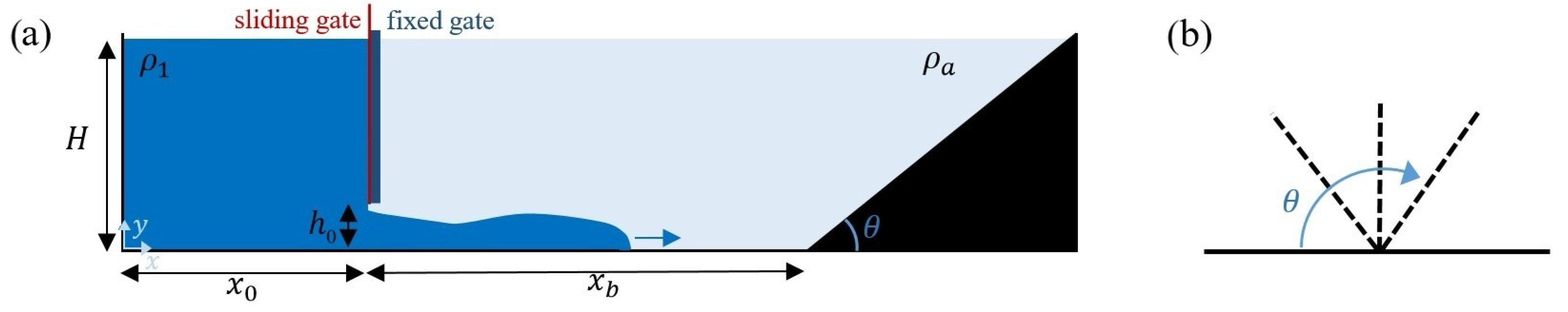
2.1. Experimental Design

The experiments were conducted at the Hydraulics Laboratory of Roma Tre University in a Perspex tank of 3 m (length), $0.3$ m (height), and $0.2$ m (width). The experimental setup, illustrated in Figure 1a, was adapted from the system described in [22] and allowed the generation of steady gravity currents. The lock reservoir was created by installing a fixed barrier at $x_0=0.4$ m, incorporating a rectangular opening at the base that spun the entire width of the tank. This opening was sealed with a thick, sliding, vertical gate.

To simulate different topographical configurations, a uniform Perspex slope was positioned at $x_b=0.85$ m downstream from the fixed barrier. The slope’s angle $\theta$ was varied to represent scenarios such as overhanging barriers, vertical obstructions, or upward slopes. The up-slope mimicked, for example, when a sea breeze meets a high ridge or a dense turbidity current meets a continental shelf or seamount. The overhang case, where the upper boundary slopes down to the floor, can occur when a dense current meets the grounding line of an ice shelf or in some geological or industrial flows, where a dense intrusion flows along the lower boundary of a contained region with a downward sloping roof [14].

For each experiment, the initial setup involved filling the first section of the tank with saline water of initial density ${\rho }_1$, while the remaining section was filled with an ambient fluid of lower density ${\rho }_a$ (${\rho }_a<{\rho }_1$), both at the same height. The experiments were carried out with a constant density difference of $\Delta \rho =40$ kg/${\mathrm{m}}^3$, where $\Delta \rho ={\rho }_1-{\rho }_a$. Initial density measurements were conducted using an electronic density meter (Anton Paar DMA 4100M, Graz, Austria), which provided an accuracy of ${10}^{-1}$${\mathrm{kg}/\mathrm{m}}^3$. To improve the visualization of the dense flow during the experiments, a precise amount of dye was added to the saline water. The choice of $\Delta \rho =40$ kg/${\mathrm{m}}^3$ was made because this value is representative of the density contrasts found in natural environments. For example, in Greenlandic fjords, the subglacial discharge of freshwater into saline basins typically produces density differences in the range of 10–50 kg/m³ [34,35]. Similar contrasts are also evident beneath Antarctic ice shelves, where meltwater mixing with seawater contributes to deep ocean mixing and large-scale circulation patterns [36,37]. Moreover, in industrial applications such as pollutant dispersion or wastewater discharge, density differences of this magnitude are commonly encountered due to variations in dissolved substances or suspended particles [38]. Selecting $\Delta \rho =40$ kg/${\mathrm{m}}^3$ ensures that the experiments operate in a Boussinesq regime, where density variations are sufficient to drive gravitational flow while remaining small enough to justify the incompressibility assumption. This controlled setting enabled a focused investigation of mixing and turbulence that was representative of many real-world scenarios.

A total of 7 experiments were conducted with a fixed gate opening of $h=0.05$ m and an initial total water depth of $H=0.3$ m. The barrier angles, $\theta$, were varied between ${30}^{\circ }$ and ${150}^{\circ }$, as illustrated in Figure 1b. The experiments and their corresponding nomenclature are summarized in

Table 1. Main parameters of the experiments performed.

Exp.	$\mathit{\theta }$	Fr	Re
B30	${30}^{\circ }$	0.82	2400
B45	${45}^{\circ }$	0.82	2400
B65	${65}^{\circ }$	0.82	2400
B90	${90}^{\circ }$	0.82	2400
B115	${115}^{\circ }$	0.82	2400
B135	${135}^{\circ }$	0.82	2400
B150	${150}^{\circ }$	0.82	2400

, along with the Froude number ($Fr$) and Reynolds number ($Re$), calculated based on the initial conditions. The Froude number was defined by $Fr={\displaystyle \frac{U}{\sqrt{g^{\prime }{h}_t}}}$, where U is the velocity of the dense flow’s front, $h_t$ is the height of the tail of the incoming gravity current, and $g^{\prime }$ is the reduced gravity. The reduced gravity was defined as $g^{\prime }=g{\displaystyle \frac{\Delta \rho }{{\rho }_a}}$, while the Reynolds number was expressed as $Re={\displaystyle \frac{U{h}_t}{\nu }}$, where $\nu$ is the kinematic viscosity of the fluid.

The experiment began with the sudden removal of a sliding gate, initiating an exchange flow through the opening. This action generated a dense gravity current that flowed from the left section of the tank to the right, while, simultaneously, a turbulent freshwater plume rose into the lock reservoir. As the gravity current advanced, it entrained the lighter fluid, leading to the dilution and mixing of the dense flow. The run concluded when the reflected gravity current, resulting from its interaction with the slope, returned and reached the location of the fixed gate.

Each run was recorded using a CCD (Charge-Coupled Device) camera operating at a frequency of 25 Hz and a spatial resolution of $1024\times 668$ pixels with a measurement accuracy of 3 mm/pixel. To achieve uniform illumination across the entire field of view, a backlight system was employed. Based on the camera resolution, we estimated a relative uncertainty of $\Delta H/H\le 4\%$, while uncertainties in the velocity and time scales were $\Delta U/U\le 2\%$ and $\Delta T/T\le 1.6\%$, respectively.

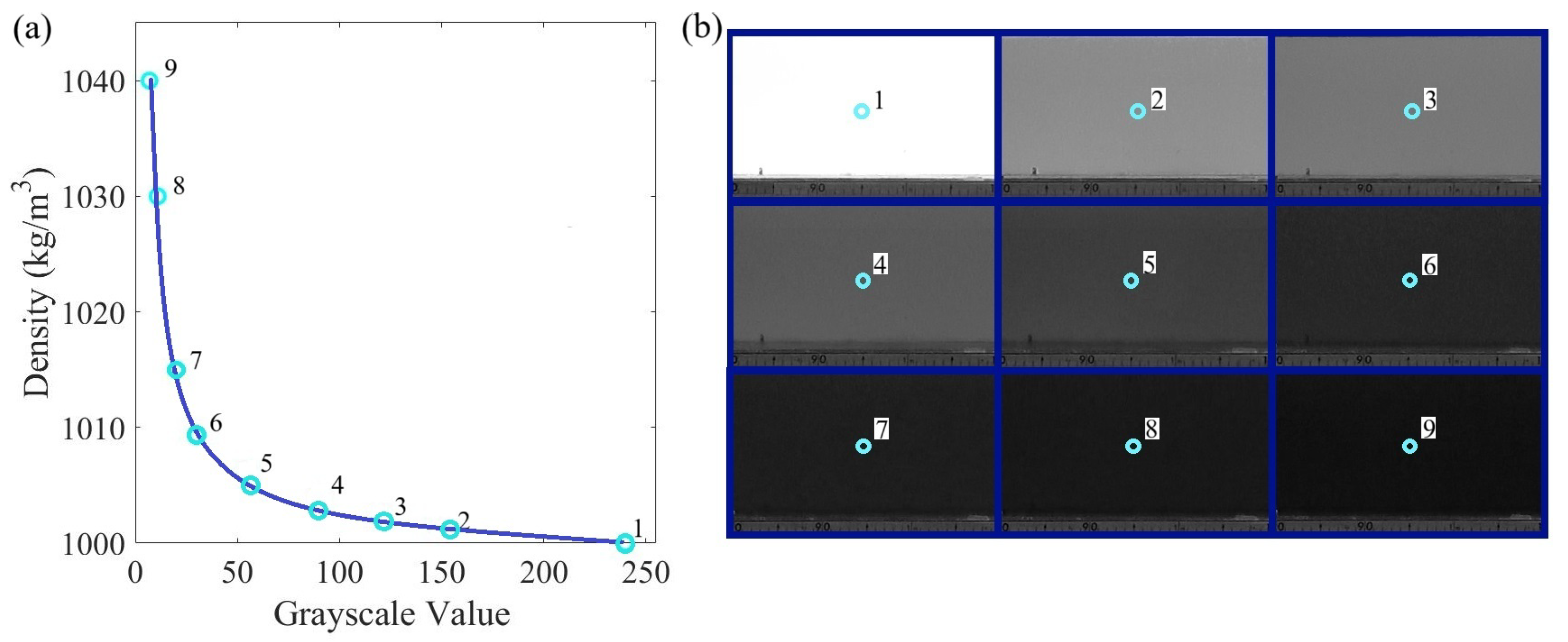
2.2. Density Evaluation Using Non-Intrusive Image Analysis

To investigate the development of the gravity current and how barriers influenced its density distribution, we obtained instantaneous width-averaged density fields through an advanced image analysis technique. This approach included a calibration process that correlated the light intensity captured in the images with the dye concentration at each pixel. The dye concentration within the flow was assumed to be linearly proportional to the salt concentration, enabling the indirect measurement of density variations in the gravity current.

A nine-step calibration procedure was implemented, in which eight controlled amounts of methylene blue dye were progressively added and mixed into fresh water to create a uniformly dyed fluid throughout the tank (Figure 2b). The dye concentration varied from zero, corresponding to the undyed ambient fluid with density ${\rho }_a$, to the maximum dye concentration in the lock reservoir with density ${\rho }_1$. For each dye concentration, including the zero-dye condition, a calibration image was captured under identical lighting conditions to ensure consistency.

The calibration curve for each pixel was generated through nonlinear interpolation, i.e., piecewise cubic polynomial interpolation of the nine acquired images (Figure 2a). Using this pixel-based calibration, the instantaneous dimensionless density field was computed as follows:

$${\rho }^{*}(x,y,t)={\displaystyle \frac{\rho (x,y,t)-{\rho }_a}{{\rho }_1-{\rho }_a}},$$

(1)

where $\rho (x,y,t)$ represents the local density of the current at any given point and time. This dimensionless representation made for easier direct comparison of density variations within the current. Figure 3 presents snapshots of the processed video images (a, c, e) alongside the corresponding dimensionless density fields (b, d, f) for run $B115$.

Analyzing the time series of grayscale values for each pixel within selected regions of the acquired frames revealed oscillations in light intensity. These variations were linked to local reflection effects and the exponential nature of the calibration curve, as the density increased with decreasing grayscale values. Both high-grayscale (“dark”) and low-grayscale (“white”) regions were examined, assessing deviations from each pixel’s temporal mean. The average density deviation was found to be $0.5\%$ in the “white” regions, while, in the “dark” regions, the deviation was more pronounced, reaching $6\%$. To correct these deviations, the mass conservation principle was applied, accounting for the total mass of both the current and the ambient fluid in the experimental tank. By applying this principle, the fluctuations caused by variations in light intensity were effectively mitigated, ensuring accurate and consistent density measurements throughout the system. The relative deviation in total mass within the tank, accounting for the initial quantities of water ($m_i$) and salt ($m_s$) introduced at the beginning of the experiment, and the total mass evaluated experimentally, was given by

$$\mathrm{Relative}\mathrm{Deviation}={\displaystyle \frac{\left|m_0-m_{\exp }\right|}{m_0}},$$

(2)

where $m_0=m_i+m_s$ is the initial total mass, and the experimentally evaluated mass was

$$m_{\exp }=z\left({\int }_{V_c}\rho (x,y,t)dV+{\int }_{V_0\left(t\right)}{\rho }_{0}dV\right)$$

(3)

Here, z is the width of the tank, $\rho (x,y,t)$ is the local density of the gravity current at time t, ${\rho }_0$ is the density of the ambient fluid, V is the total volume considered per unit width of the tank, and $V_c\left(t\right)$ and $V_0\left(t\right)$ are the volumes of the gravity current and ambient fluid per unit width of the tank, respectively. This method enabled a comparison of the mass in the tank over time with the initial mass introduced into the system.

In essence, the mass conservation principle effectively mitigated the impact of light fluctuations, ensuring the reliability of the density evaluation, despite the inverse relationship between grayscale values and fluid density in the experimental setup.

The reliability of the applied methods could be assessed by comparing the initial mass of salt introduced into the lock region with the total salt mass estimated from the instantaneous density distribution obtained through image analysis. The error observed varied between $10\%$ and $15\%$, with the most significant discrepancies occurring in thinner gravity currents. This higher error in thin currents is likely attributable to the smaller volume of dense fluid, which made the measurements more sensitive to uncertainties related to light intensity fluctuations, calibration curve precision, and the spatial resolution limitations of the imaging system.

3. Discussion

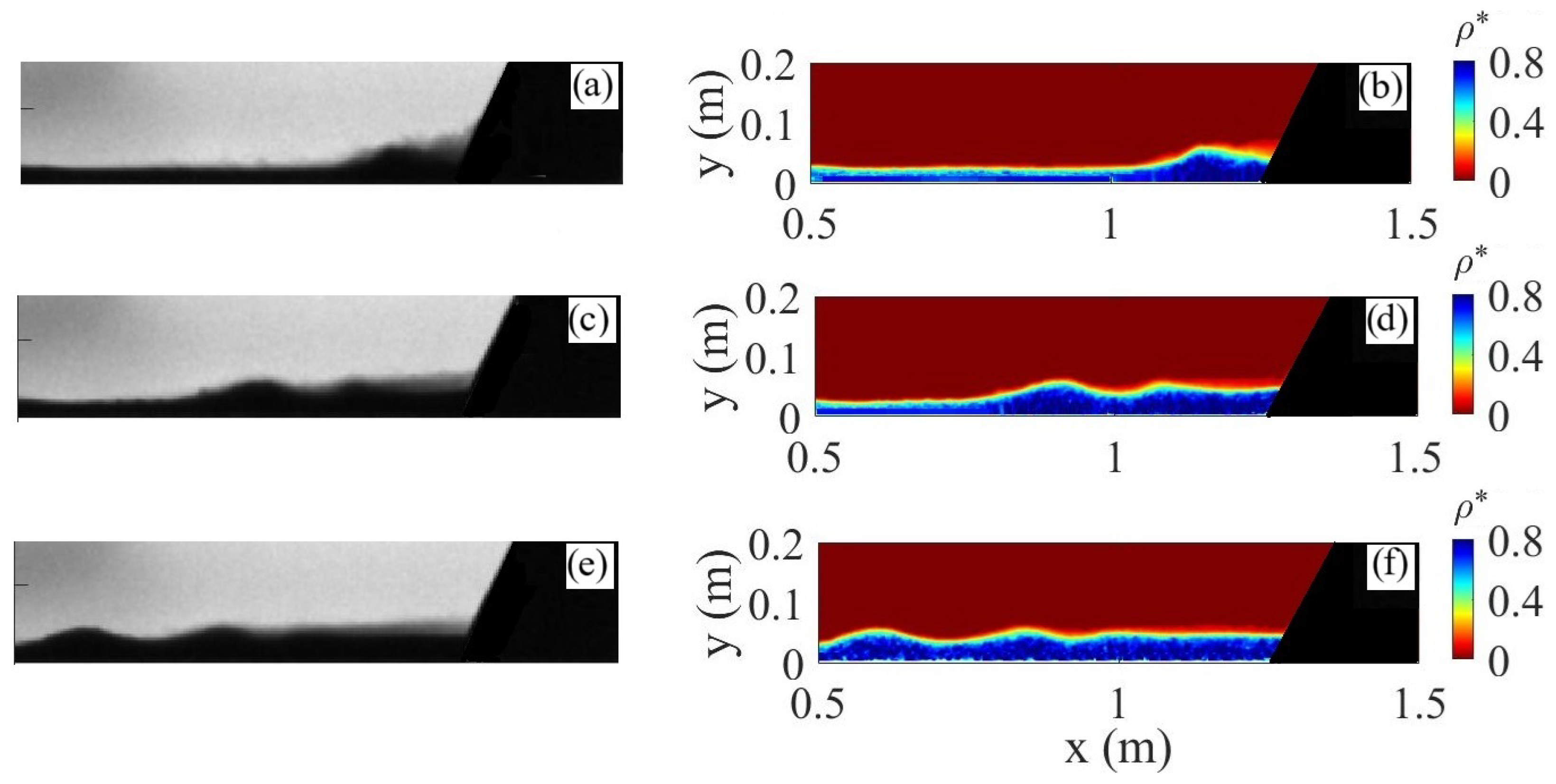
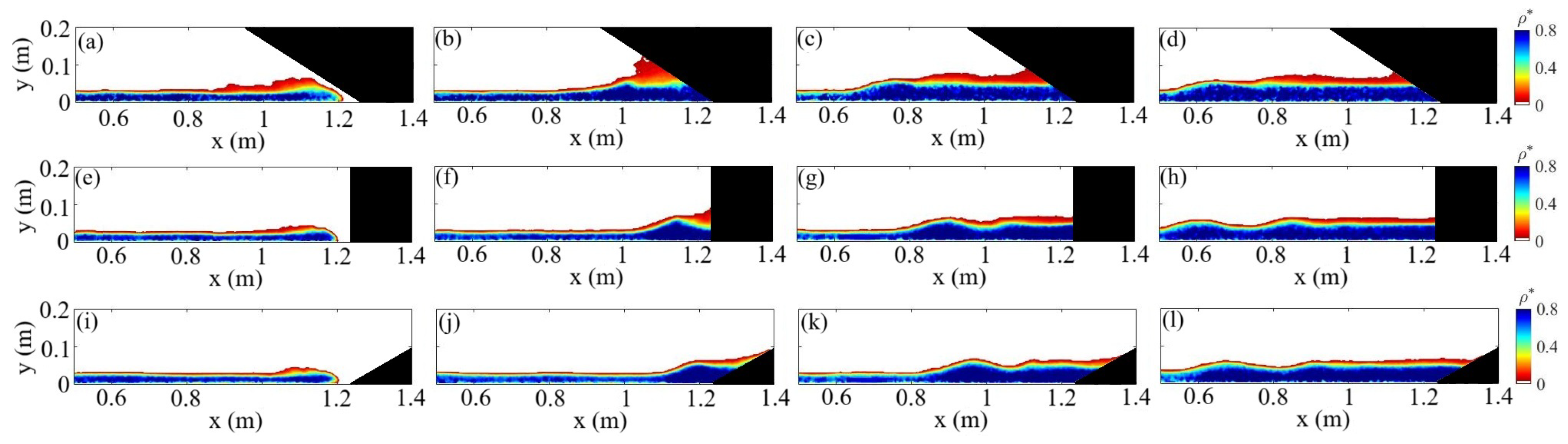
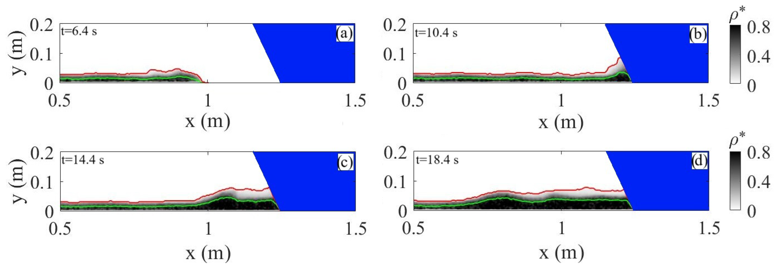
3.1. Visual Insights into Flow Development

The instantaneous density fields showed that the barrier strongly affected the dynamics of the gravity current and the reflection process. Upon release, the flow exhibited the typical structure of a density current, forming a distinct head, body, and tail before interacting with the barrier (Figure 4a,e,i). Upon reflection, a fluid bore was generated, moving in the opposite direction, with a mixing zone near the barrier (Figure 4b,f,j), and subsequently breaking down into a series of smooth waveforms (Figure 4c,d,g,h,k,l). The shape and size of the reflected bore were closely related to the incoming gravity current [39], and [17], demonstrated that the characteristics of internal bores are influenced by the ratio $h_b/h_t$, where $h_b$ represents the mean thickness of the fluid within the bore and $h_t$ is the thickness of the lower fluid layer before the bore’s arrival. Based on this ratio, internal bores could be classified as follows:

When $1<h_b/h_t<2$, the bore exhibited a smooth, undular form with no significant disturbances. For $2<h_b/h_t<4$, the bore remained undular, though shear instability at the rear of the waves caused some mixing. Finally, when $h_b/h_t>4$, the bore took on characteristics of a density current, resembling a dense flow.

In our case study, $h_t\approx 0.03$ m and $h_b\approx 0.06$ indicated the presence of an undular bore characterized by mixing phenomena at the interface. Varying $\theta$ revealed distinct dynamics near the barrier.

While the current approached the barrier, its head was deflected upward. For $\theta >{90}^{\circ }$, the current slowed as it moved up the slope, causing the head to thin. A reflected bore propagated upstream (Figure 4j), while a transient splash rose further until it reached its maximum height. In contrast, for $\theta \le {90}^{\circ }$, the lift forces exerted by the impinging gravity current on the interface were notably stronger. The smaller the slope inclination, the more pronounced the mixing became.

Figure 5 provides zoomed-in views of experiments $B30$ (a), $B45$ (b), $B65$ (c), $B90$ (d), $B115$ (e), $B135$ (f), and $B150$ (g) at the moment when the dense current interacted with the barrier and reached its maximum vertical height. The black lines, representing the $2\%$ and $50\%$ dimensionless isopycnal, highlight the differing behaviors and variations in the height of the dense current near the barrier.

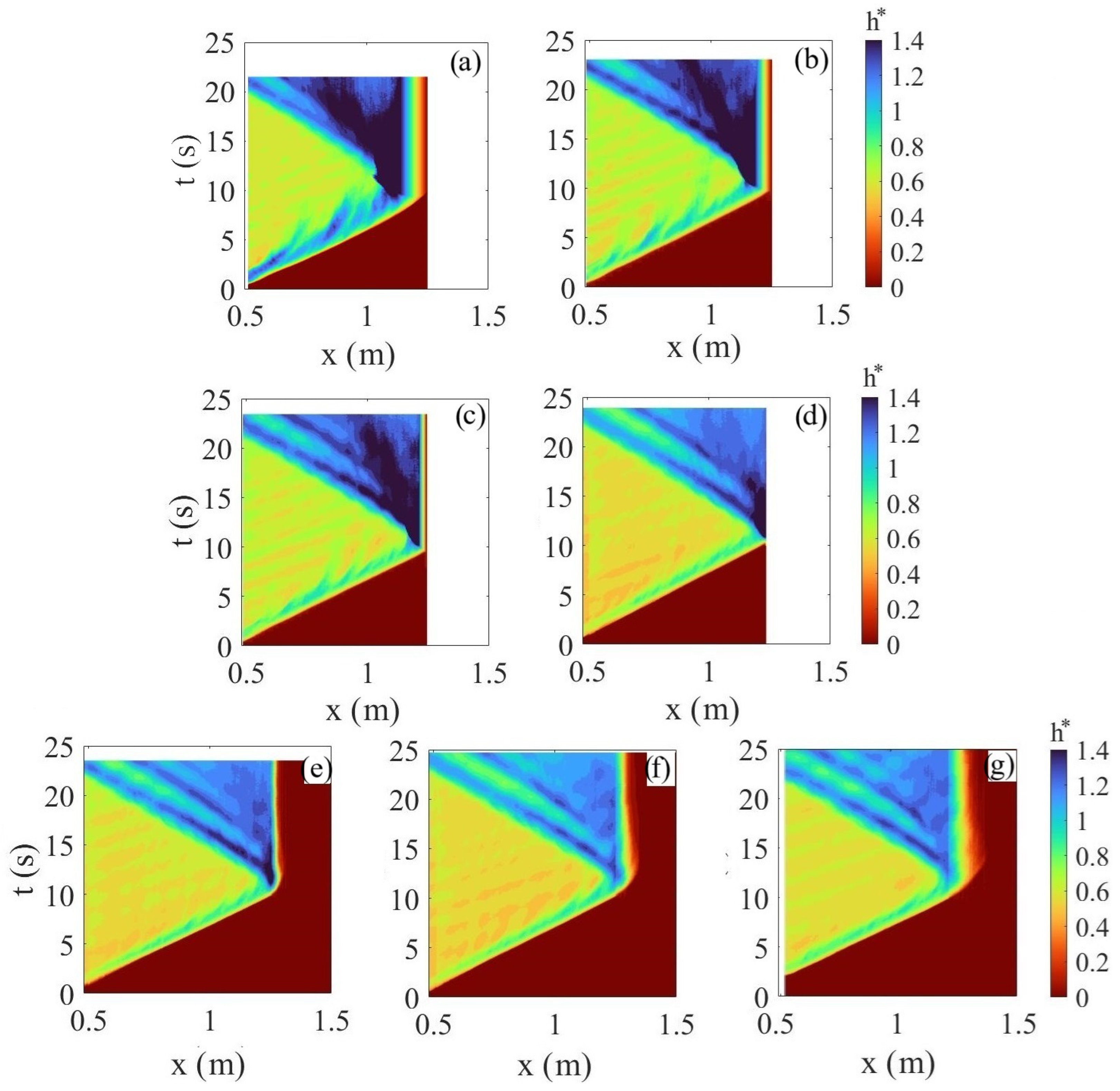
3.2. Height Variations of the Dense Gravity Current

A dimensionless density of $2\%$ was used to define the interface between the dense and light fluids and the current thickness, as in [4,14]. The non-dimensional thickness of the current, $h^{*}=h(x,t)/h_0$, is shown in Figure 6 for all the experiments performed. The front of the current, marked by the transition from the fully red region to the colormap area, exhibited a linear variation in time until it reached the toe of the barrier. Additionally, the alternation of dark blue and light green stripes after $t<10$ s clearly indicated the undular bore generated by the reflection of the dense current (see, for instance, Figure 6e).

The higher $h^{*}$ values observed during the experiments corresponded to the outgoing bores and head region, characterized by turbulent instabilities, such as Kelvin–Helmholtz instabilities, visible as height discontinuities along the current. For $\theta >{90}^{\circ }$ (Figure 6e–g), both the Kelvin–Helmholtz instabilities and the $h^{*}$ values of the reflected bore appeared lower compared to the cases where $\theta \le {90}^{\circ }$. The $h^{*}$ was strongly influenced by the barrier. An increase in $h^{*}$ was evident near the toe of the barrier, highlighted by the darker shades of blue in Figure 6, representing the portion of the current reflected upstream by the obstacle.

As suggested by the Hovmöller diagrams for runs with $\theta \le {90}^{\circ }$ (Figure 6a–d), the dark stripes indicated regions where greater depth-averaged height, $h^{*}$, was more evident. The highest ‘splash’ occurred for $\theta ={30}^{\circ }$ (Figure 6a); as the dense current approached the barrier, it was influenced by the variation in free surface height. In this case, even the Kelvin–Helmholtz instabilities became more pronounced. Conversely, as $\theta$ increased, the variations in $h^{*}$ were gradually attenuated.

Ref. [29] defined a different theshold $h_s(x,t)$ as follows:

$$h_{\mathrm{s}}(x,t)={\displaystyle \frac{g}{g_0^{\prime }}}\int {\displaystyle \frac{\rho (x,y,t)-{\rho }_a}{{\rho }_1}}dy$$

(4)

If the interface between the fluids was well defined with no mixing, $h_s(x,t)$ would represent the exact height of the interface at each horizontal position. However, mixing reduced the local density and diffused the interface, causing $h_s(x,t)$ to be smaller than the current height defined by the $2\%$ threshold.

Figure 7 shows the dimensionless density field at four different times for the run $B65$. The red line represents the current height, h, calculated using the $2\%$ dimensionless isopycnal, while the green line indicates the Shin height, $h_s$. It can be observed that below $h_s$, the current appeared unaffected by local mixing phenomena. Following the interaction between the dense current and the barrier (Figure 7b–d), the difference between h and $h_s$ increased. This difference further grew during the formation of the reflected current behind the bore (Figure 7c,d) compared to the initial phase of the dense current’s advance (Figure 7a).

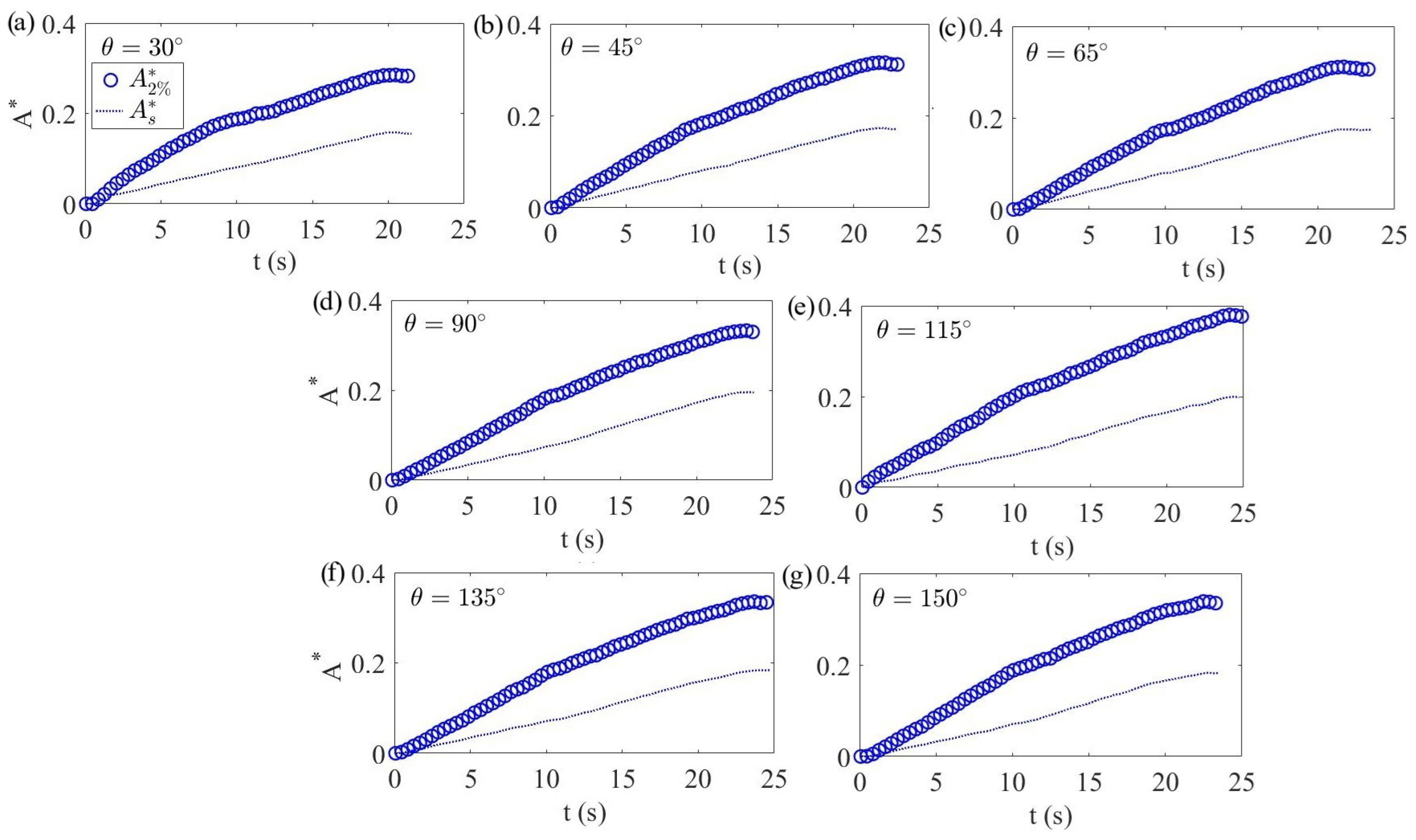
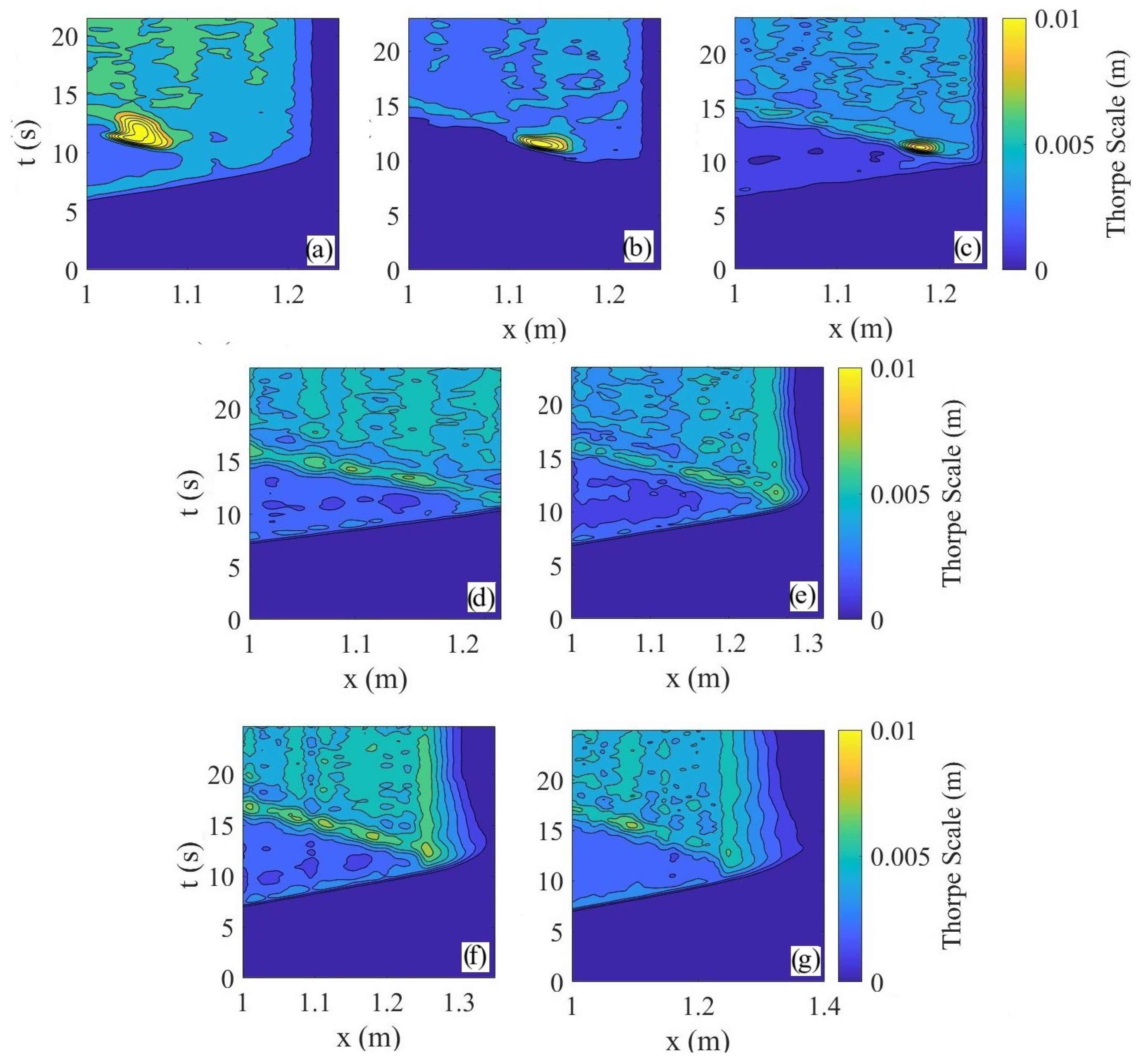
3.3. Mixing Induced by the Barriers: Fractional Area and Thorpe Length

The behavior of gravity currents was significantly affected by energy loss caused by turbulence and the mixing interactions between the current and the surrounding fluid. Along its path, the gravity current entrained fresh water, increasing its volume, and the evaluation of this increase could be used to investigate the entrainment processes within the dense current. Following the works of [40,41,42], the non-dimensional area of the dense current, $A^{*}$, per unit width, was defined as

$$A^{*}\left(t\right)={\displaystyle \frac{A_i-A_0}{A_0}},$$

(5)

where $A_i$ represents the bulk area of the dense current in the $x-y$ plane at time $t_i$ and $A_0$ is the initial area of the lock’s dense fluid. $A^{*}$ was evaluated both as the area of the dense current under the iso-density level $\rho =2\%$ ($A_{2\%}^{*}$) and as the area of the current identified by the Shin height ($A_s^{*}$). In Figure 8, both values are displayed as a function of the dimensional time t for all the experiments performed. Focusing on $A_{2\%}^{*}$, it was observed that for almost all the experiments, the area of the current increased linearly up to approximately $t>10\mathrm{s}$. This trend was not observed for $\theta ={30}^{\circ }$ (Figure 8a), where the gravity current was influenced by the barrier from the very beginning. The reduction in the free surface height, due to the small angle of the barrier, resulted in a slowdown of the gravity current and led to a more pronounced area development along the vertical direction, even before the gravity current directly interacted with the barrier.

As for $A_s^{*}$, this represented the area of the gravity current unaffected by turbulent mixing. In this case, slightly lower values were observed for $\theta ={30}^{\circ }$ (Figure 8a), while no notable differences were observed in the other experiments.

A method to estimate dissipation and diffusion rates is the Thorpe-scaling method. The Thorpe scale ($L_T$), introduced by [43], provides a measure of the turbulent mixing intensity in stratified fluids. It is derived by analyzing density profiles, such as those obtained from CDT (Conductivity–Temperature–Depth) measurements, and estimating the vertical displacement of fluid parcels required to form a stable density profile. In this method, the observed density profile, ${\rho }_n$, is “Thorpe-sorted” to obtain a monotonically stable profile, ${\widehat{\rho }}_n$, where

$$y_n\left({\rho }_n\right)\to {\widehat{y}}_n\left({\rho }_n\right),$$

(6)

and ${\widehat{\rho }}_{n+1}<{\widehat{\rho }}_n$ ensures stability.

The Thorpe scale is defined as the root mean square (RMS) of the vertical shifts between the initial and rearranged depths for each sample within a turbulent zone:

$$L_T={〈{\left(y_n-{\widehat{y}}_n\right)}^2〉}^{1/2},$$

(7)

where n represents the set of samples within the patch, $y_n$ is the original depth, ${\widehat{y}}_n$ is the depth after sorting, and $\langle ·\rangle$ denotes averaging over the patch.

Physically, $L_T$ quantifies the intensity of turbulence by measuring the magnitude of vertical displacements required to stabilize the density profile. Larger values of $L_T$ indicate stronger turbulent mixing, and it is often used as a proxy for estimating turbulent energy dissipation rates or mixing efficiency.

In our case study, the analysis was conducted using instantaneous vertical density fields. Figure 9 presents the Thorpe scale, $L_T$, as a function of the spatial coordinate (x) and time (t) for the runs $B30$ (a), $B45$ (b), $B65$ (c), $B90$ (d), $B115$ (e), $B135$ (f), and $B150$ (g). The results revealed that the impact of the dense current on the barrier at angles $\theta <{90}^{\circ }$ generated stronger turbulent mixing localized near the toe of the barrier, which subsequently dissipated over time.

In contrast, for cases with $\theta \ge {90}^{\circ }$, the values of $L_T$ associated with the impact of the dense current on the slope were lower in magnitude. However, these cases exhibited continuous vertical displacements over time, clearly illustrating the mixing induced by the reflected bore. This distinct behavior highlighted the dependence of turbulent mixing intensity and spatial distribution on the interaction angle between the dense current and the barrier.

To analyze the local behavior near the barrier, Figure 10 presents the maximum Thorpe scale, $L_T$, for the same runs shown in Figure 9. This zoomed-in view clearly demonstrates that the maximum $L_T$ was observed in run $B30$ (Figure 10a), with a progressive decrease in $L_T$ as $\theta$ increased. Another noteworthy observation was the shift of the maximum $L_T$ along the x-axis as $\theta$ increased for $\theta$ values between ${30}^{\circ }$ and ${90}^{\circ }$ (Figure 10a–d). For the remaining runs, the maximum $L_T$ remained nearly constant across the x-coordinate (Figure 10e,f). These results highlighted the influence of the interaction angle on both the intensity and spatial distribution of turbulent mixing near the barrier.

4. Conclusions

This study explored the interaction between gravity currents and inclined barriers, emphasizing the crucial role of barrier inclination in shaping mixing dynamics. Using a novel, non-intrusive image analysis technique to measure density variations, our experiments revealed that barriers influence the gravity current even before direct impact, altering both reflection patterns and turbulent mixing. The results show that barrier inclination significantly affects both the vertical displacement of the current and the intensity of turbulence, with lower-angle barriers ($\theta \le {90}^{\circ }$) inducing stronger localized mixing compared to steeper configurations. This enhanced mixing at lower-angle barriers can be attributed to stronger shear layer interactions and more efficient energy conversion. When a gravity current encounters a gently sloping barrier, the abrupt flow deflection intensifies shear, triggering Kelvin–Helmholtz instabilities that fragment the flow and amplify turbulence. This rapid conversion of kinetic energy into turbulent energy accelerates dissipation and enhances ambient fluid entrainment, leading to more vigorous, localized mixing near the barrier. In contrast, steeper barriers produce a more gradual flow deceleration, resulting in weaker shear layers and lower turbulence intensity, thereby limiting mixing efficiency.

The experimental results highlight a clear trend in the intensity of localized mixing as a function of barrier inclination. While bulk measurements of the non-dimensional area $A^{*}$ provided a general overview of the current’s evolution, the Thorpe scale analysis offered a more detailed assessment of turbulent intensity. Specifically, the Thorpe scale analysis showed that barriers inclined at $\theta ={30}^{\circ }$ generated the highest turbulent mixing, with maximum values of $L_T$ reaching approximately $40\%$ higher than those observed for a $\theta ={90}^{\circ }$ barrier. For intermediate angles such as $\theta ={45}^{\circ }$ and $\theta ={65}^{\circ }$, the increase in mixing intensity remained significant but followed a decreasing trend as the inclination angle grew. In contrast, barriers inclined at $\theta ={115}^{\circ }$ or steeper exhibited a marked reduction in turbulence generation, with $L_T$ values dropping by nearly $50\%$ compared to the lowest-angle configurations. These findings provide a quantitative framework for predicting how different barrier angles modulate mixing dynamics, offering valuable insights for both environmental and engineering applications.

Beyond laboratory conditions, these findings have direct implications for estuarine and coastal systems. Gravity currents play a key role in sediment transport, pollutant dispersion, and mixing in natural environments, and our results suggest that engineered structures—such as dikes, breakwaters, and other hydraulic barriers—can be strategically designed to control mixing dynamics. For instance, in flood management, steeper barriers may help preserve stratification and reduce unwanted mixing, minimizing sediment resuspension and maintaining water quality. Conversely, where increased mixing is beneficial, such as in pollutant dilution or sediment resuspension for navigation, lower-inclination barriers may offer a more effective solution.

The relevance of these insights extends to industrial applications where controlled mixing is critical. In sediment management and water treatment systems, understanding how barrier geometry influences turbulence can inform the optimization of settling tanks and reactors. Integrating these experimental observations into numerical models can enhance predictive capabilities for environmental risk management and the design of more efficient coastal and industrial infrastructures.

References

1. Simpson, J.E. Gravity Currents: In the Environment and the Laboratory; Cambridge University Press: Cambridge, UK, 1997. [Google Scholar]
2. Cesare, G.D.; Schleiss, A.; Hermann, F. Impact of turbidity currents on reservoir sedimentation. J. Hydraul. Eng. 2001, 127, 6–16. [Google Scholar]
3. Prather, B.E. Controls on reservoir distribution, architecture and stratigraphic trapping in slope settings. Mar. Pet. Geol. 2003, 20, 529–545. [Google Scholar]
4. De Falco, M.; Adduce, C.; Maggi, M. Gravity currents interacting with a bottom triangular obstacle and implications on entrainment. Adv. Water Resour. 2021, 154, 103967. [Google Scholar]
5. De Falco, M.C.; Adduce, C.; Cuthbertson, A.; Negretti, M.E.; Laanearu, J.; Malcangio, D.; Sommeria, J. Experimental study of uni-and bi-directional exchange flows in a large-scale rotating trapezoidal channel. Phys. Fluids 2021, 33, 036602. [Google Scholar]
6. Maggi, M.R.; Negretti, M.E.; Hopfinger, E.J.; Adduce, C. Turbulence characteristics and mixing properties of gravity currents over complex topography. Phys. Fluids 2023, 35, 016607. [Google Scholar]
7. Maggi, M.R.; Negretti, M.E.; Martin, A.; Naaim-Bouvet, F.; Hopfinger, E.J. Experimental study of gravity currents moving over a sediment bed: Suspension criterion and bed forms. Environ. Fluid Mech. 2024, 24, 1215–1233. [Google Scholar]
8. Maggi, M.; Hopfinger, E.; Sommeria, J.; Adduce, C.; Viboud, S.; Valran, T.; Negretti, M. Laboratory experiments of rotating stratified exchange flows over a sediment bed. Adv. Water Resour. 2025, accepted. [Google Scholar]
9. Dai, A.; Huang, Y.L. Experiments on gravity currents propagating on unbounded uniform slopes. Environ. Fluid Mech. 2020, 20, 1637–1662. [Google Scholar] [CrossRef]
10. Dai, A.; Huang, Y.L. Boussinesq and non-Boussinesq gravity currents propagating on unbounded uniform slopes in the deceleration phase. J. Fluid Mech. 2021, 917, A23. [Google Scholar]
11. De Falco, M.C.; Adduce, C.; Negretti, M.E.; Hopfinger, E.J. On the dynamics of quasi-steady gravity currents flowing up a slope. Adv. Water Res. 2021, 147, 103791. [Google Scholar]
12. Maggi, M.R.; Adduce, C.; Negretti, M.E. Lock-release gravity currents propagating over roughness elements. Environ. Fluid Mech. 2022, 22, 383–402. [Google Scholar] [CrossRef]
13. He, Z.; Han, D.; Lin, Y.T.; Zhu, R.; Yuan, Y.; Jiao, P. Propagation, mixing, and turbulence characteristics of saline and turbidity currents over rough and permeable/impermeable beds. Phys. Fluids 2022, 34, 066604. [Google Scholar] [CrossRef]
14. Maggi, M.; Adduce, C.; Lane-Serff, G. Gravity currents interacting with slopes and overhangs. Adv. Water Resour. 2023, 171, 104339. [Google Scholar] [CrossRef]
15. Wu, C.S.; Dai, A. Gravity currents from a constant inflow on unbounded uniform slopes. J. Hydraul. Res. 2023, 61, 880–892. [Google Scholar] [CrossRef]
16. Di Lollo, G.; Adduce, C.; Brito, M.; Ferreira, R.M.; Ricardo, A.M. Turbulent kinetic energy redistribution in a gravity current interacting with an emergent cylinder. Adv. Water Resour. 2024, 183, 104585. [Google Scholar] [CrossRef]
17. Edwards, D.; Leeder, M.; Best, J.; Pantin, H. On experimental reflected density currents and the interpretation of certain turbidites. Sedimentology 1994, 41, 437–461. [Google Scholar] [CrossRef]
18. Kneller, B.; McCaffrey, W. Depositional effects of flow nonuniformity and stratification within turbidity currents approaching a bounding slope; deflection, reflection, and facies variation. J. Sediment. Res. 1999, 69, 980–991. [Google Scholar] [CrossRef]
19. Skevington, E.W.; Hogg, A.J. The unsteady overtopping of barriers by gravity currents and dam-break flows. J. Fluid Mech. 2023, 960, A27. [Google Scholar] [CrossRef]
20. Greenspan, H.P.; Young, R.E. Flow over a containment dyke. J. Fluid Mech. 1978, 87, 179–192. [Google Scholar] [CrossRef]
21. Rottman, J.; Simpson, J.; Hunt, J.; Britter, R. Unsteady gravity current flows over obstacles: Some observations and analysis related to the phase II trials. J. Hazard. Mater. 1985, 11, 325–340. [Google Scholar] [CrossRef]
22. Lane-Serff, G.; Beal, L.; Hadfield, T. Gravity current flow over obstacles. J. Fluid Mech. 1995, 292, 39–53. [Google Scholar]
23. Gonzalez-Juez, E.; Meiburg, E.; Constantinescu, G. Gravity currents impinging on bottom-mounted square cylinders: Flow fields and associated forces. J. Fluid Mech. 2009, 631, 65–102. [Google Scholar]
24. Pickering, K.T.; Hiscott, R.N. Contained (reflected) turbidity currents from the Middle Ordovician Cloridorme Formation, Quebec, Canada: An alternative to the antidune hypothesis. In Deep-Water Turbidite Systems; Wiley: Hoboken, NJ, USA, 1991; pp. 89–110. [Google Scholar]
25. Pickering, K.T.; Underwood, M.B.; Taira, A. Open-ocean to trench turbidity-current flow in the Nankai Trough: Flow collapse and reflection. Geology 1992, 20, 1099–1102. [Google Scholar] [CrossRef]
26. Baines, P. Upstream blocking and airflow over mountains. Annu. Rev. Fluid Mech. 1987, 19, 75–95. [Google Scholar]
27. Barry, M.E.; Ivey, G.N.; Winters, K.B.; Imberger, J. Measurements of diapycnal diffusivities in stratified fluids. J. Fluid Mech. 2001, 442, 267–291. [Google Scholar]
28. Smyth, W.; Moum, J.; Caldwell, D. The efficiency of mixing in turbulent patches: Inferences from direct simulations and microstructure observations. J. Phys. Oceanogr. 2001, 31, 1969–1992. [Google Scholar]
29. Shin, J.; Dalziel, S.; Linden, P. Gravity currents produced by lock exchange. J. Fluid. Mech. 2004, 521, 1–34. [Google Scholar]
30. Ivey, G.; Winters, K.; Koseff, J. Density stratification, turbulence, but how much mixing? Annu. Rev. Fluid Mech. 2008, 40, 169–184. [Google Scholar]
31. Bouffard, D.; Boegman, L. A diapycnal diffusivity model for stratified environmental flows. Dyn. Atmos. Ocean. 2013, 61, 14–34. [Google Scholar] [CrossRef]
32. Yih, C.S.; Guha, C. Hydraulic jump in a fluid system of two layers. Tellus 1955, 7, 358–366. [Google Scholar]
33. Wood, I.; Simpson, J. Jumps in layered miscible fluids. J. Fluid Mech. 1984, 140, 329–342. [Google Scholar]
34. Everett, A.; Kohler, J.; Sundfjord, A.; Kovacs, K.M.; Torsvik, T.; Pramanik, A.; Boehme, L.; Lydersen, C. Subglacial discharge plume behaviour revealed by CTD-instrumented ringed seals. Sci. Rep. 2018, 8, 13467. [Google Scholar] [CrossRef]
35. Jackson, C. Freshwater flux from subglacial discharge and its impact on fjord circulation in Greenland. Geophys. Res. Lett. 2017, 44, 5500–5508. [Google Scholar]
36. Joughin, I.; Alley, R.B. Stability of the West Antarctic ice sheet in a warming world. Nat. Geosci. 2011, 4, 506–513. [Google Scholar] [CrossRef]
37. Jenkins, A.; Jacobs, S. Sub-ice shelf melting and ocean circulation in Antarctica. J. Geophys. Res. Ocean. 2008, 113, C04013. [Google Scholar] [CrossRef]
38. Fischer, H.; List, J.E.; Koh, C.R.; Imberger, J.; Brooks, N.H. Mixing in Inland and Coastal Waters; Academic Press: New York, NY, USA, 1979. [Google Scholar]
39. Rottman, J.W.; Simpson, J.E. The formation of internal bores in the atmosphere: A laboratory model. Q. J. R. Meteorol. Soc. 1989, 115, 941–963. [Google Scholar]
40. Jacobson, M.R.; Testik, F.Y. On the concentration structure of high-concentration constant-volume fluid mud gravity currents. Phys. Fluids 2013, 25, 016602. [Google Scholar]
41. Ottolenghi, L.; Adduce, C.; Inghilesi, R.; Armenio, V.; Roman, F. Entrainment and mixing in unsteady gravity currents. J. Hydraul. Res. 2016, 54, 541–557. [Google Scholar]
42. Adduce, C.; Maggi, M.R.; De Falco, M.C. Non-intrusive density measurements in gravity currents interacting with an obstacle. Acta Geophys. 2022, 70, 2499–2510. [Google Scholar]
43. Thorpe, S. A laboratory study of stratified accelerating shear flow over a rough boundary. J. Fluid Mech. 1984, 138, 185–196. [Google Scholar]
Figure 1. (a) Illustration of the experimental setup. (b) Reference frame for the barrier angles.
Water 17 01062 g001
Figure 2. (a) Calibration curve constructed using nine images, with each image corresponding to a controlled and known dye concentration. (b) Calibration images representing the nine dye concentrations used to determine the correlation between grayscale intensity and dye concentration in the calibration process.
Water 17 01062 g002
Figure 3. Experimental images (a,c,e) and dimensionless density fields for the same times (b,d,f) of run B 115 .
Water 17 01062 g003
Figure 4. Dimensionless density fields for runs B 30 (ad), B 90 (eh), and B 150 (il) at t = 9.5 s (a,e,i), t = 13.5 s (b,f,j), t = 17.5 s (c,g,k), and t = 21.5 s (d,h,l).
Water 17 01062 g004
Figure 5. Zoomed-in views of non-dimensional density fields near the barrier for runs B 30 (a), B 45 (b), B 65 (c), B 90 (d), B 115 (e), B 135 (f), and B 150 (g). The black lines represent the 2 % and 50 % dimensionless isopycnal, highlighting the local variations in the dense current’s height near the barrier.
Water 17 01062 g005
Figure 6. Dimensionless height of the current h * for the experiments B 90 (a), B 30 (b), B 45 (c), B 65 (d), B 115 (e), B 135 (f), and B 150 (g).
Water 17 01062 g006
Figure 7. Dimensionless density ρ * for run B 65 at four different times. The red line represents the current height calculated using the 2 % dimensionless isopycnal, while the green line indicates the Shin height h s ( x , t ) , computed according to Equation (4).
Water 17 01062 g007
Figure 8. Time evolution of the non-dimensional dense current area, A * , for all the experiments performed. The empty blue circles represent the area of the dense current under the iso-density level ρ = 2 % ( A 2 % * ), while the dashed line indicates the area of the current identified by the Shin height ( A s * ).
Water 17 01062 g008
Figure 9. Thorpe scale ( L T ) map illustrating the temporal and spatial variations of mixing intensity for runs B 30 (a), B 45 (b), B 65 (c), B 90 (d), B 115 (e), B 135 (f), and B 150 (g).
Water 17 01062 g009
Figure 10. Profiles of the maximum Thorpe scale value ( L T ) for the spatial range x = 1 m to x = 1.4 m across the runs B 30 (a), B 45 (b), B 65 (c), B 90 (d), B 115 (e), B 135 (f), and B 150 (g).
Water 17 01062 g010