Interpretable Machine Learning Based Quantification of the Impact of Water Quality Indicators on Groundwater Under Multiple Pollution Sources

Abstract

Accurate evaluation of groundwater quality and identification of key characteristics are essential for maintaining groundwater resources. The purpose of this study is to strengthen water quality evaluation through the SHAP and XGBoost algorithms, analyze the key indicators affecting water quality in depth, and quantify their impact on groundwater quality through interpretable tools. The XGBoost algorithm shows that zinc (0.183), nitrate (0.159), and chloride (0.136) are the three indicators with the highest weight. The SHAP algorithm shows that zinc (34.62%), nitrate (17.65%), and chloride (16.98%) have higher contribution values, which explains the output results of XGBoost. According to the calculation scores and classification standards of the water quality model, 49% of the groundwater samples in the study area have excellent water quality, 33% of the samples are better, and 18% of the samples are polluted. The results of positive matrix factorization (PMF) show that natural conditions, metal processing, metal smelting and mining, and agricultural activities all cause pollution to groundwater. Zinc, chloride, nitrate, and manganese were the key variables determined by the SHAP algorithm to explain the vast majority of human health risk sources. These findings indicate that interpretable machine learning not only improves the correlation of water quality assessment but also quantifies the judgment basis of each sample and helps to track key pollution indicators.

1. Introduction

Groundwater pollution has evolved into a global water environment problem [1]. Fluoride, nitrate, iron, manganese, antibiotics, and even pathogenic microorganisms are present in groundwater systems in many parts of the world, leading to a deterioration in water quality [2,3,4]. Industrialization, urbanization, and population concentration make groundwater quality threatened by complex pollution sources [5,6,7]. In addition, a large number of studies have shown that the use of contaminated groundwater will significantly increase the probability of human disease [8,9,10]. It is challenging to objectively determine water quality under complex external conditions, analyze pollution sources, assess the impact of groundwater on human health, and identify risk sources.

The water quality index (WQI) is a widely used comprehensive water quality assessment method [11]. The water quality results are obtained by weighting and scoring the selected indicators, applying the aggregation function to calculate, and classifying them [12]. Some early studies have shown that the WQI model is affected by the subjectivity of the researchers, and the water quality results are biased [13]. Among them, due to the frequent use of the Delphi method [14], the determination of the index weight link has strong subjectivity. As an advanced data processing method, machine learning has been gradually applied to determine the weight of water quality indicators to reduce the subjective bias in WQI models [15].

Common validations of machine learning applications are mostly carried out in terms of results, based on metrics such as accuracy and R² [16,17]. For black-box models or high-dimensional models, it is inaccurate to test the effectiveness of model application by assessment metrics alone [18]. The application of complex machine learning models still lacks transparency and interpretability, and researchers can only see the results of the model application and cannot explain the basis on which the model makes its judgments [19,20], which poses an uncontrollable and challenging situation for the deep application of machine learning in the groundwater domain. In WQI modeling, researchers often apply the weighting results obtained by machine learning algorithms targeting binary classification directly after assessment, ignoring the principles of the algorithms themselves in practice, which reduces the transparency and interpretability of water quality assessment results. Lee et al. [21] used the random forest algorithm to assign weights and developed a standard process for the WQI model. Lap [22] and others think that machine learning algorithms are very effective in dealing with complex nonlinear relational data. Four algorithms, including support vector machine, random forest, decision tree, and multi-layer perceptron, are studied. It is found that these methods have good effects in the process of water quality evaluation.

The weights of the water quality indicators, which are key for the model to determine the water quality status and make predictions, are obtained through the relationship between the water quality datasets. The degree to which a human can predict the outcome of a model or understand the reasons for its decisions is referred to as interpretability. Explainable machine learning (XAI) is able to deeply analyze the model’s learning results from both global and local perspectives, and demonstrate the basis of the model’s judgments through the data, which facilitates researchers to identify the key factors, thus making the application of machine learning more reasonable and explainable, which improves the credibility [23,24,25]. Jeong et al. [26] used interpretable machine learning to predict the salinity in groundwater, quantify the influence of pathogenic factors on the salinity in groundwater, and successfully determine the factors of groundwater salinization.

Unclean groundwater is hazardous to human health if it is used in scenarios such as agricultural irrigation, drinking, bathing and washing, and cooking [7]. The accumulation of toxins from year to year can gradually affect human health conditions by inducing conditions such as skin diseases, diarrhea, muscle weakness, vomiting and allergic reactions, and even cancer [27,28]. Therefore, human health risk assessment for groundwater is necessary. Groundwater contamination is multi-source; industrial activities, agricultural activities, residential life, and plant and animal decay can contaminate groundwater [29]. Industrialization, urbanization, and population activities are the main sources of pollution, which, together with the disturbances in the hydrogeological environment, make the sources of risk complex and difficult to find [30]. The PMF (positive matrix factorization) model belongs to the multivariate statistical analysis model, the basic core of which is to distinguish the characteristics and contributions of different pollution sources in the mixed model. Although this method has not been applied much in the field of groundwater pollution traceability, it has been shown that the application is more effective and can be of great help in tracing the pollution sources.

The main purpose of this study is to apply interpretable machine learning algorithms to improve the water quality evaluation model, further explore the application and performance evaluation of machine learning in water quality evaluation, calculate and analyze the impact of multiple water quality indicators on human health in the study area, and determine the source of risk.

2. Materials and Methods

2.1. Study Area

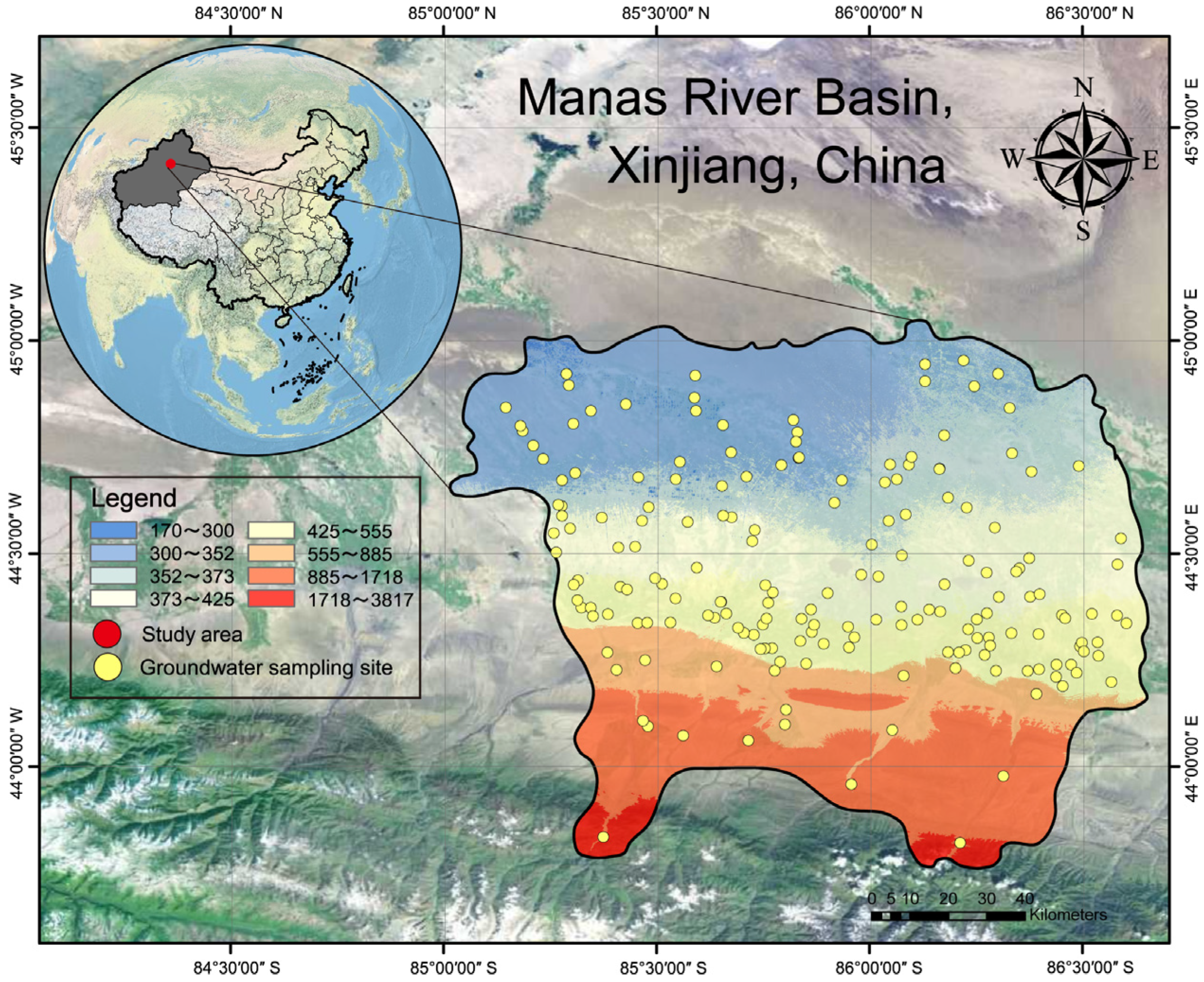
In this study, part of the Manas River Basin in Xinjiang Province, China, was used as the study area (Figure 1). The Manas River Basin is located at the southern edge of the Junggar Basin and the middle part of the northern foothills of the Tianshan Mountains in the Xinjiang Uygur Autonomous Region. The surface conditions in the study area are complex, including a variety of landforms such as mountains, oases, and deserts [31]. Precipitation in the region tends to decrease from south to north and is concentrated in April to August each year, accounting for 55% of the total annual precipitation. The length of the Manas River is about 400 km, the total annual runoff in the basin is 1.0~1.5 billion m³, and 750 million m³ of groundwater can be extracted under normal conditions [32]. The study area is located in the economic zone of the northern slope of the Tianshan Mountains, which is a key economic zone for development, with rapid development of agriculture, animal husbandry, and industry, including industrial enterprises such as metal smelting and processing, leather processing, and mining extraction, and the population of inhabitants grows year by year [33].

2.2. Sample Collection and Analysis

The data used in this study were obtained from groundwater samples collected from the Manas River Basin in 2019. Based on the results of the investigation of pollution sources and the investigation of the surrounding environment of groundwater in the study area, combined with the local hydrogeological conditions and the existing groundwater sampling points and information, sampling points were set up in the surrounding areas of various pollution sources, river systems, and areas that were not obviously affected. A total of 187 groundwater sampling sites were selected in the study area. To ensure that the water samples were representative, the monitoring wells were pumped and cleaned for sampling. Five 500 mL sampling bottles were used to collect water samples at each site, four for water quality testing and one for blank control, and were sent to the testing laboratory within 24 h. Sensory trait indicators such as pH, conductivity, and turbidity were measured in situ by an Aqua Troll 500 Multiparameter Sonde (In-Situ, Fort Collins, CO, USA), with an error of less than 10%; detection of the major anions and cations were analyzed using the laboratory’s in-house ion chromatograph (PIC-10), with an error of less than 5%.

2.3. XWQI Model Construction Based on Explainable Machine Learning

Based on the traditional WQI model, this study uses an explainable machine learning algorithm to improve it, enhance the overall interpretability of the water quality evaluation model, and deepen the application and understanding of machine learning in the water quality evaluation process, so as to construct a water quality index model based on explainable machine learning (XWQI). 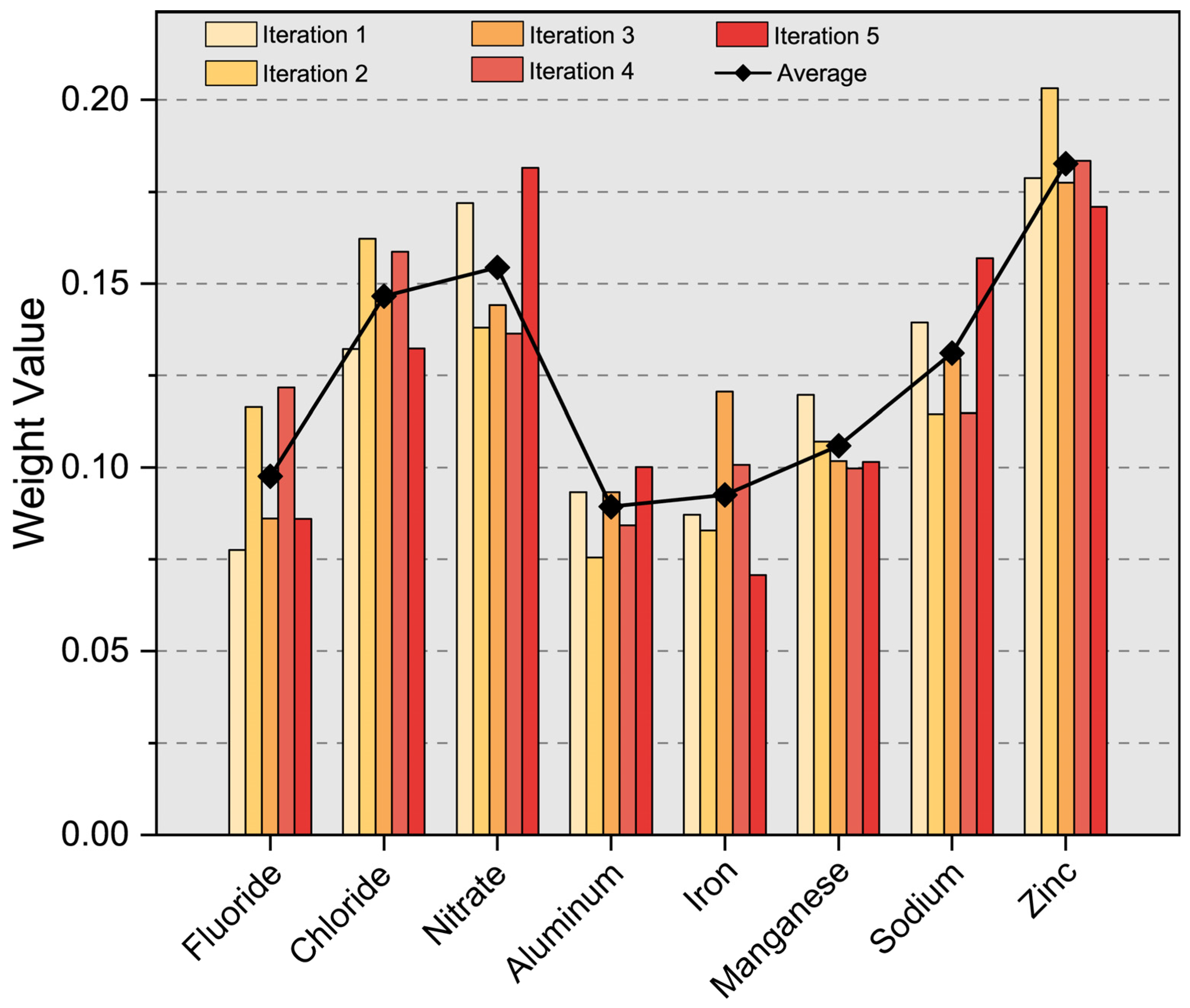The XWQI model consists of a total of four basic steps [34]: (a) indicator selection, (b) subindicator scoring, (c) determination of indicator weights, and (d) aggregation. In this study, the determination of indicator weights is improved with advanced machine learning methods based on the traditional WQI.

Through chemical analysis of groundwater quality samples, a dataset consisting of 35 water quality indicators including chloride, nitrate, and zinc was obtained. When there are too many water quality indicators, it is easy to disperse the weight value, reduce the impact of key water quality indicators on water quality, and interfere with the results of water quality evaluation. In order to reflect the impact of pollution indicators on water quality to the greatest extent, this study selected the indicators with over-standard phenomena as the dataset of water quality indicators for constructing the XWQI based on the groundwater quality standards promulgated by China.

In order to select a suitable machine learning algorithm to construct a water quality rating model, this study selected three white-box models: KNN, logistic regression, and support vector machines, and three black-box models: XGBoost, AdaBoost, and RNN, with accuracy as the key indicator for preliminary screening.

Preprocessing of the datasets is an important part of ensuring the effectiveness of machine learning and improving interpretability [35]. The outliers of the indicators were screened to remove the noise due to non-water quality factors such as improper operation of the sampling process. The initial state of the points was determined by comparing the indicator measurements with the groundwater quality standards published in China, thus using a one-way discriminant method (

Table 1. Standard threshold of the water quality indicators used for groundwater.

Indicator	Unit	Standard Threshold
Fluoride	mg/L	1
Chloride	mg/L	250
Nitrate	mg/L	10
Aluminum	mg/L	0.2
Iron	mg/L	0.3
Manganese	mg/L	0.1
Sodium	mg/L	200
Zinc	mg/L	1

). The initial state of each point was used as an input term for binary classification by XGBoost. The sub-indicator function was used to convert the measured values of the water quality indicators to dimensionless values, with higher scores indicating higher concentrations of the indicator in the water body (Equation (1)), and the aggregation function was used to calculate the water-quality results (Equation (2)), where C_i represents the concentration, P_i represents the threshold, SI_i represents the indicator score, Score represents the water quality assessment result, and W_i represents the indicator weight.

$${SI}_i={\displaystyle \frac{C_i}{P_i}}$$

(1)

$$Score={\sum }_{i=1}^n{W}_i\times {SI}_i$$

(2)

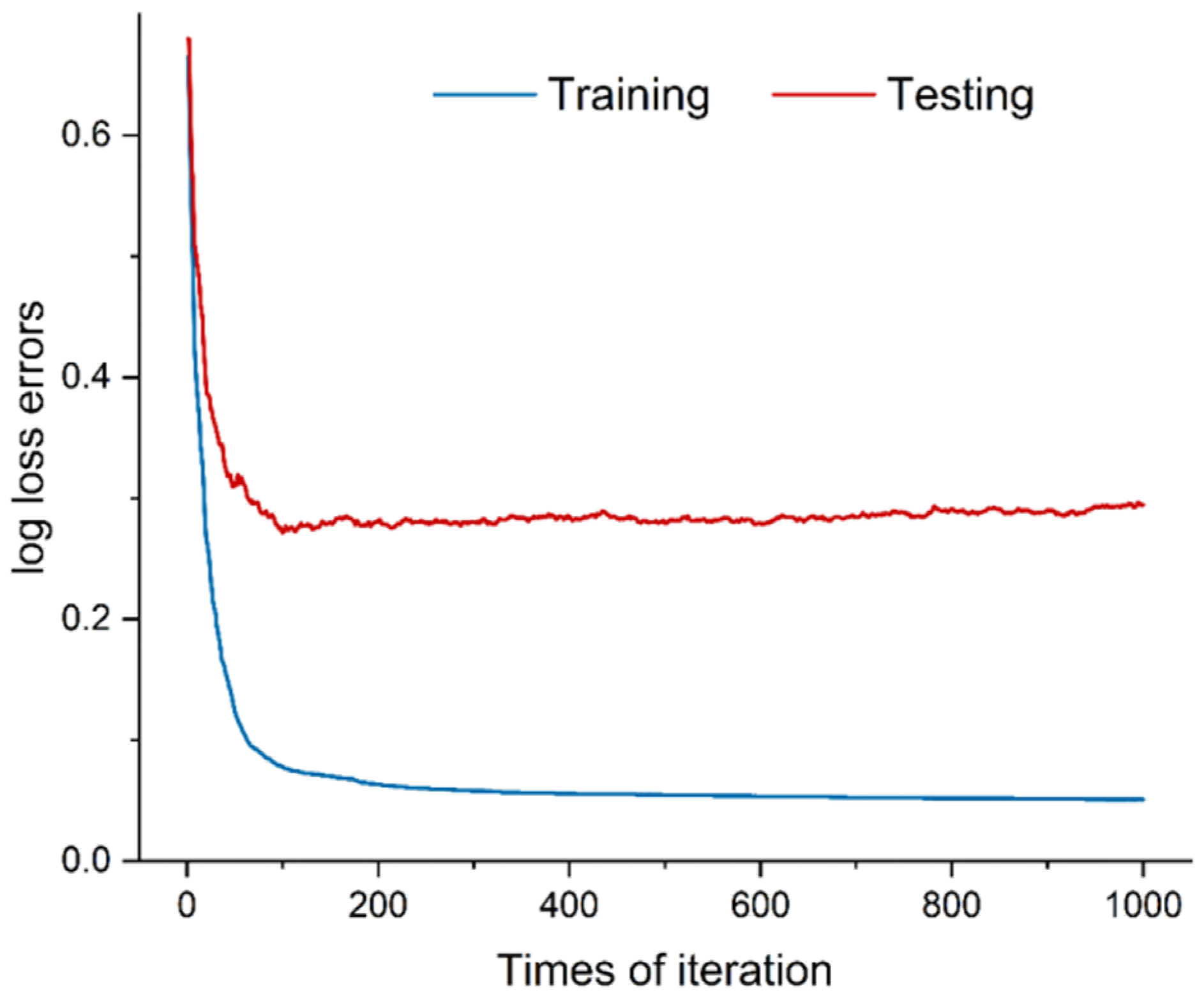
XGBoost is a more complex black-box model, which is prone to problems such as over-fitting and thus leads to a poor validation of the test set [36]. The goal of XGBoost is to minimize the loss function under an additive predictive model. For a given dataset (x_i, y_i), where x_i is the feature vector and y_i is the objective value, the model can be represented as a combination of multiple weak learners (usually decision trees). A regularity term is set up for XGBoost, which is used to penalize the model complexity (Equation (4)) and a loss function Equation (3).

$$f_t\left(x\right)=w_{q\left(x\right)} , w\in R^T, q:R^d\to \left\{\mathrm{1,2},\cdots ,T\right\}$$

(3)

$$L\left(\theta \right)=\sum _i\left[y_i\mathit{ln}\left(1+e^{-\widehat{y_i}}\right)+\left(1-y_i\right)\mathit{ln}\left(1+e^{\widehat{y_i}}\right)\right]$$

(4)

Based on the loss function and the regular term, the objective function is set as Equation (5).

$${Obj}^{\left(t\right)}=\sum _{i=1}^{n}l\left(y_i,{\widehat{y}}_i^{\left(t-1\right)}+f_t\left(x_i\right)\right)+\Omega \left(f_t\right)+constant$$

(5)

After Taylor expansion and approximation as in Equation (6), the first- and second-order derivatives of the loss function are calculated at each step, the objective function is optimized, and the resulting tree model is summed.

$${Obj}^{\left(t\right)}=\sum _{i=1}^n\left[g_i{f}_i\left(x_i\right)+{\displaystyle \frac{1}{2}}{h}_i{f}_t^2\left(x_i\right)\right]+\Omega \left(f_t\right)$$

(6)

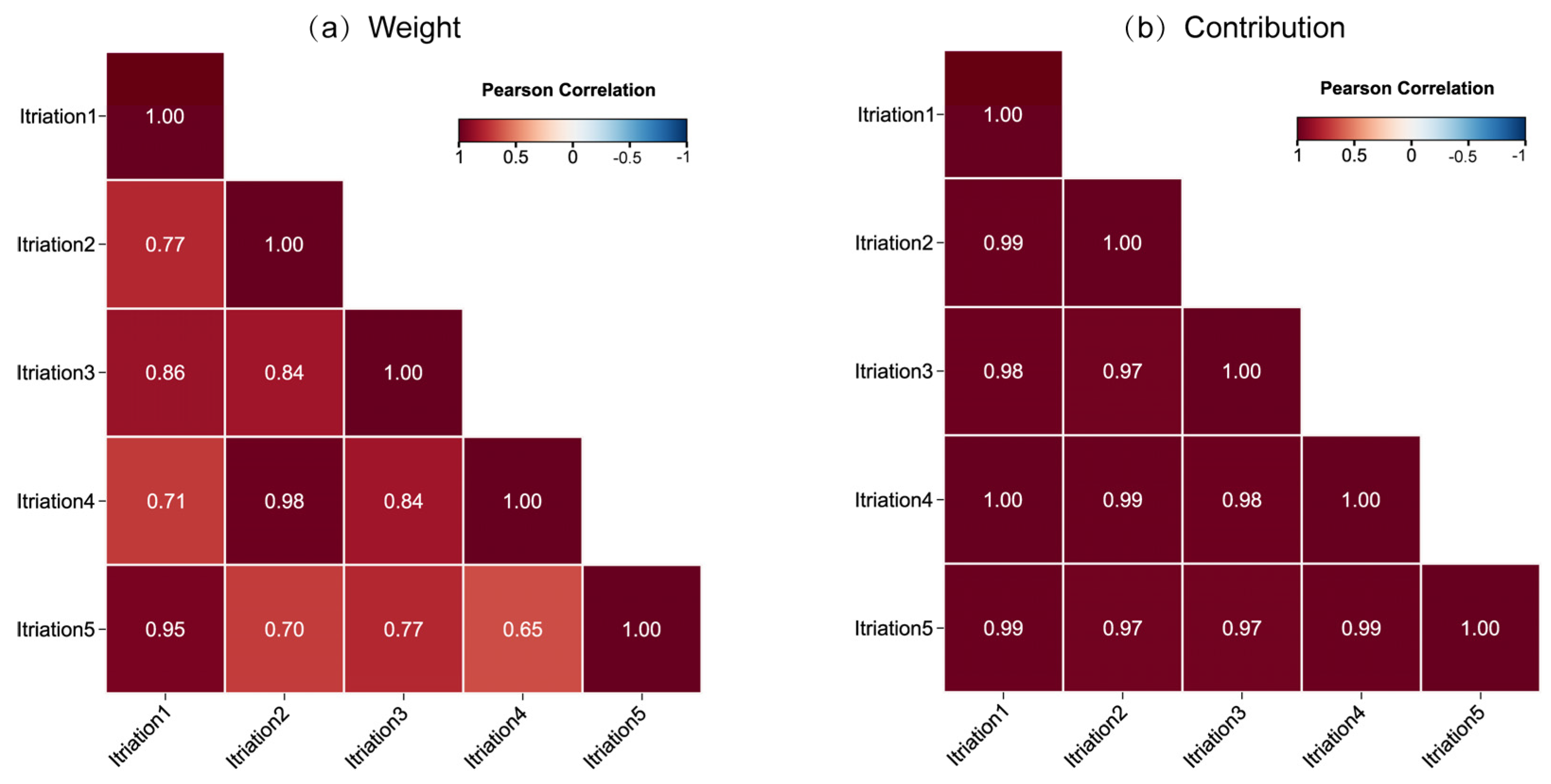
K-fold cross-validation is a common method to prevent overfitting. This method re-divides the new datasets for learning and testing within the training set and repeats it k times. To improve the model performance for the datasets, a grid search algorithm is used to adjust the hyper-parameters.

2.4. Interpretability Analysis

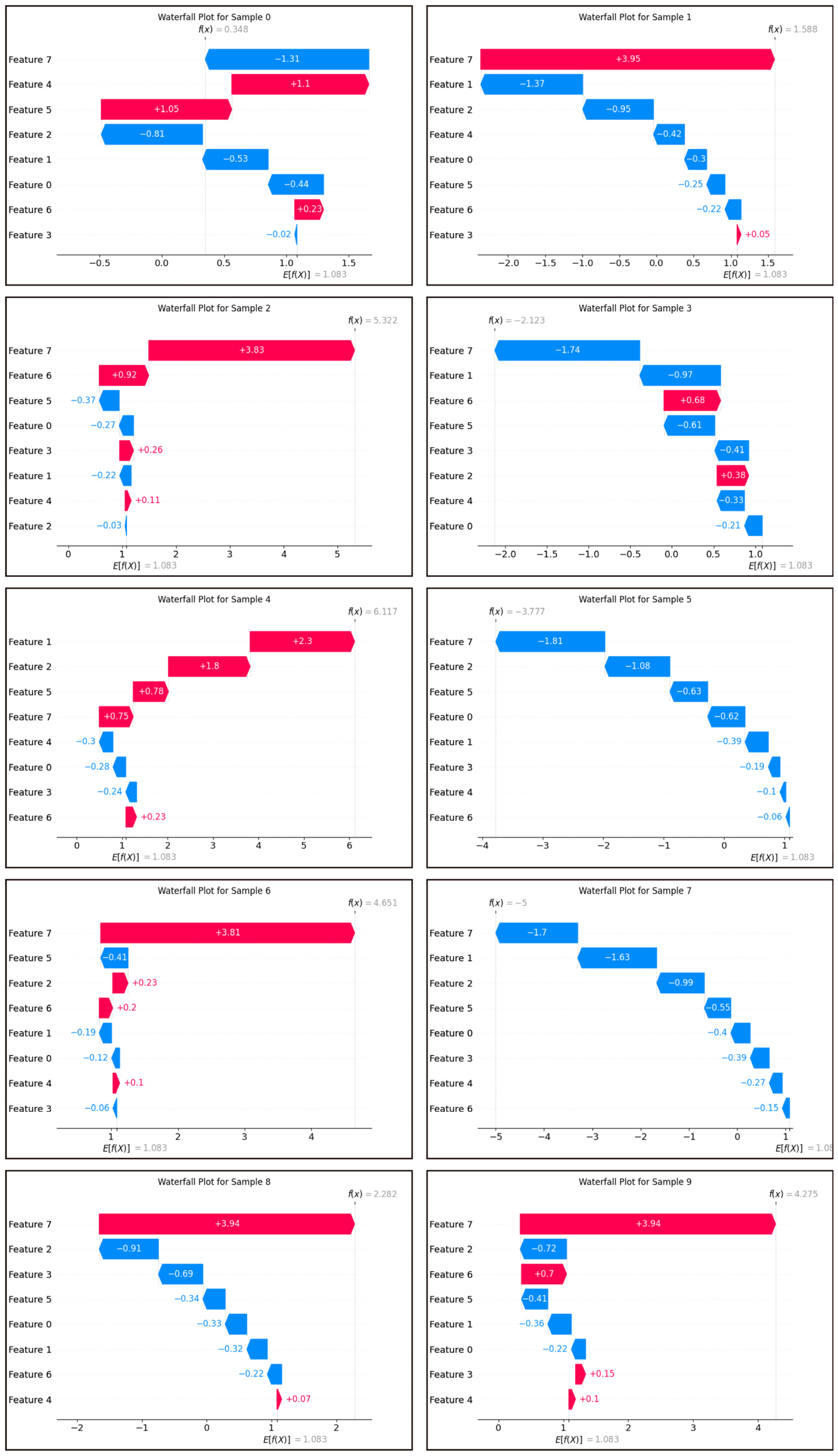
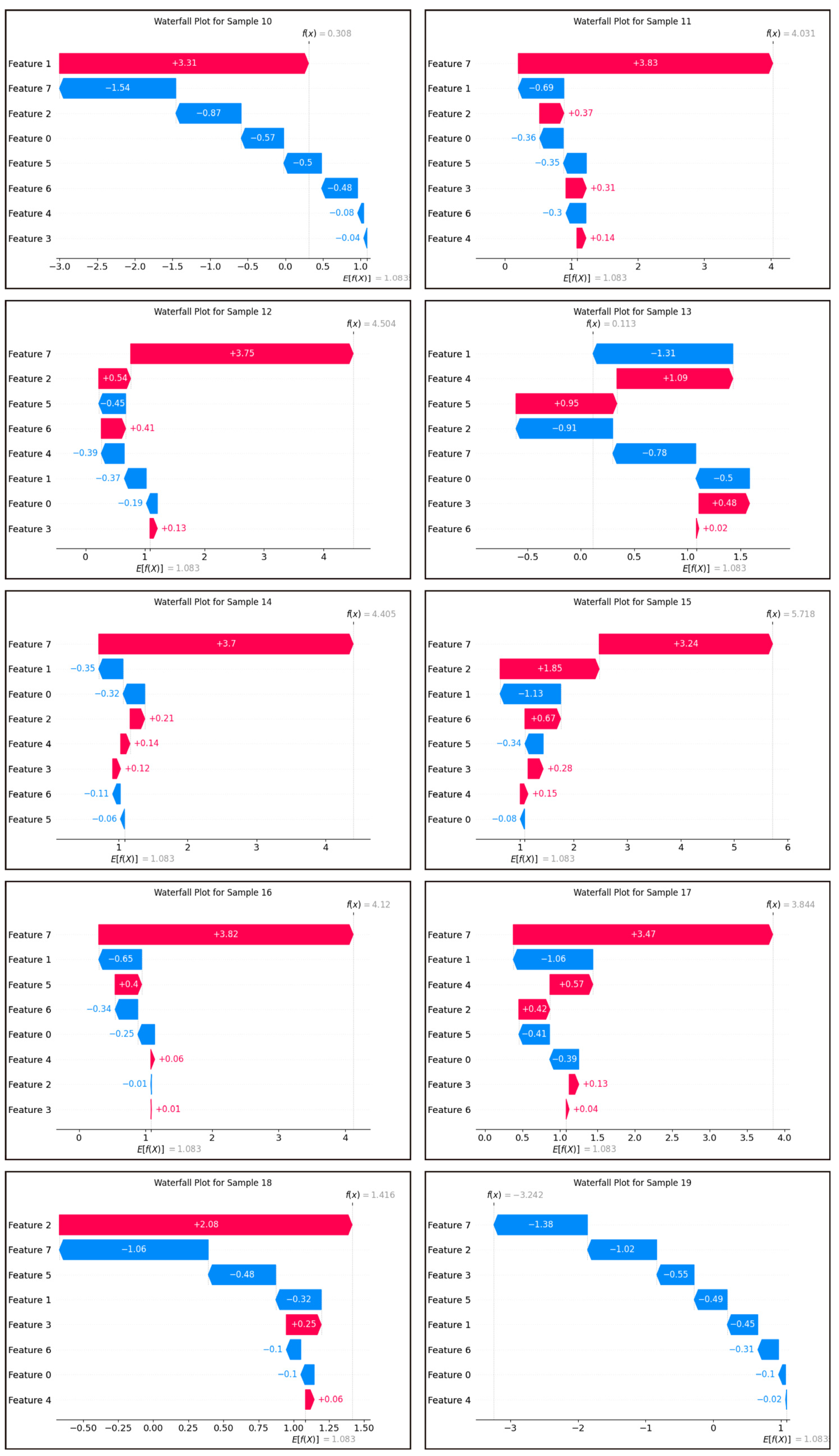
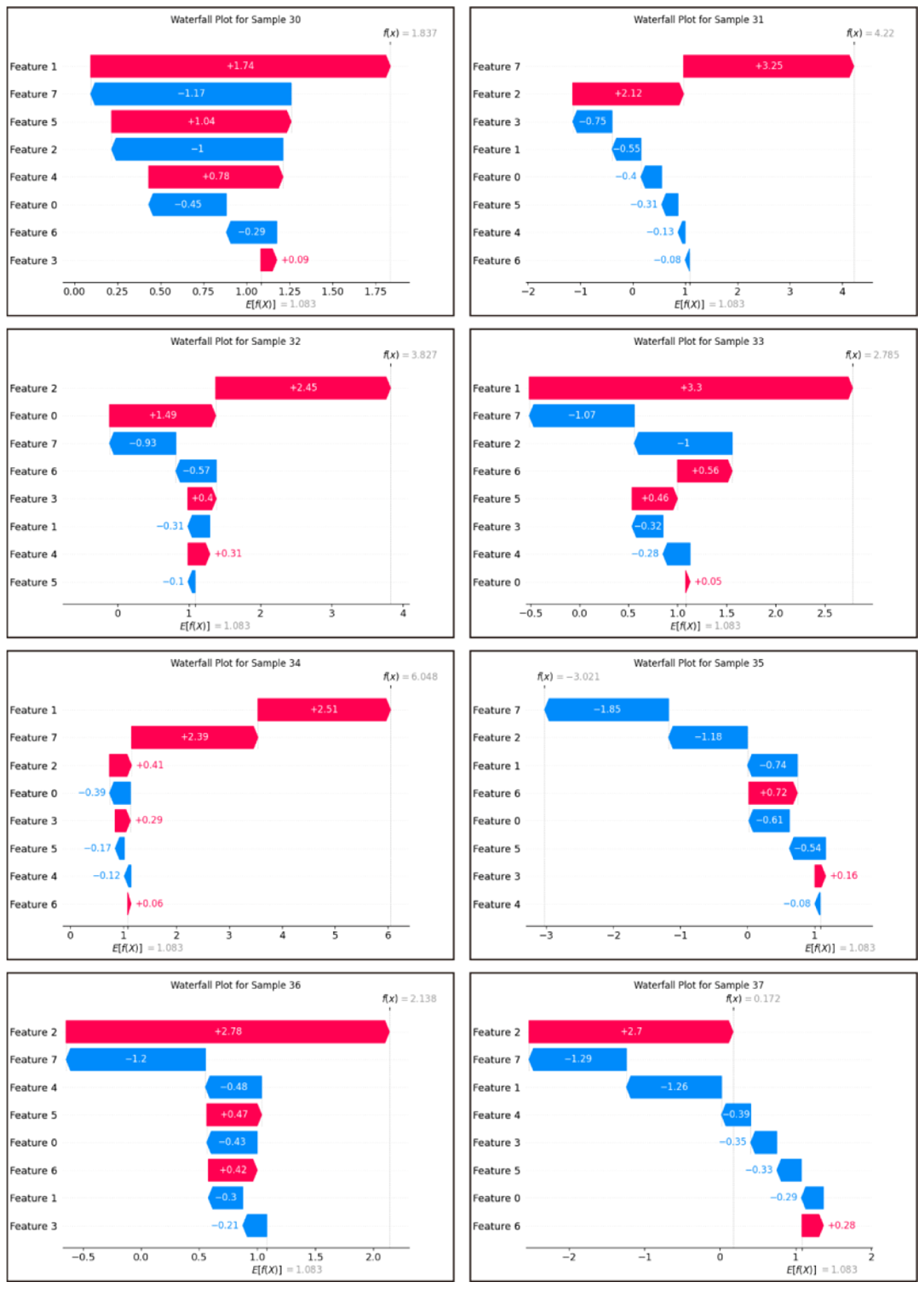
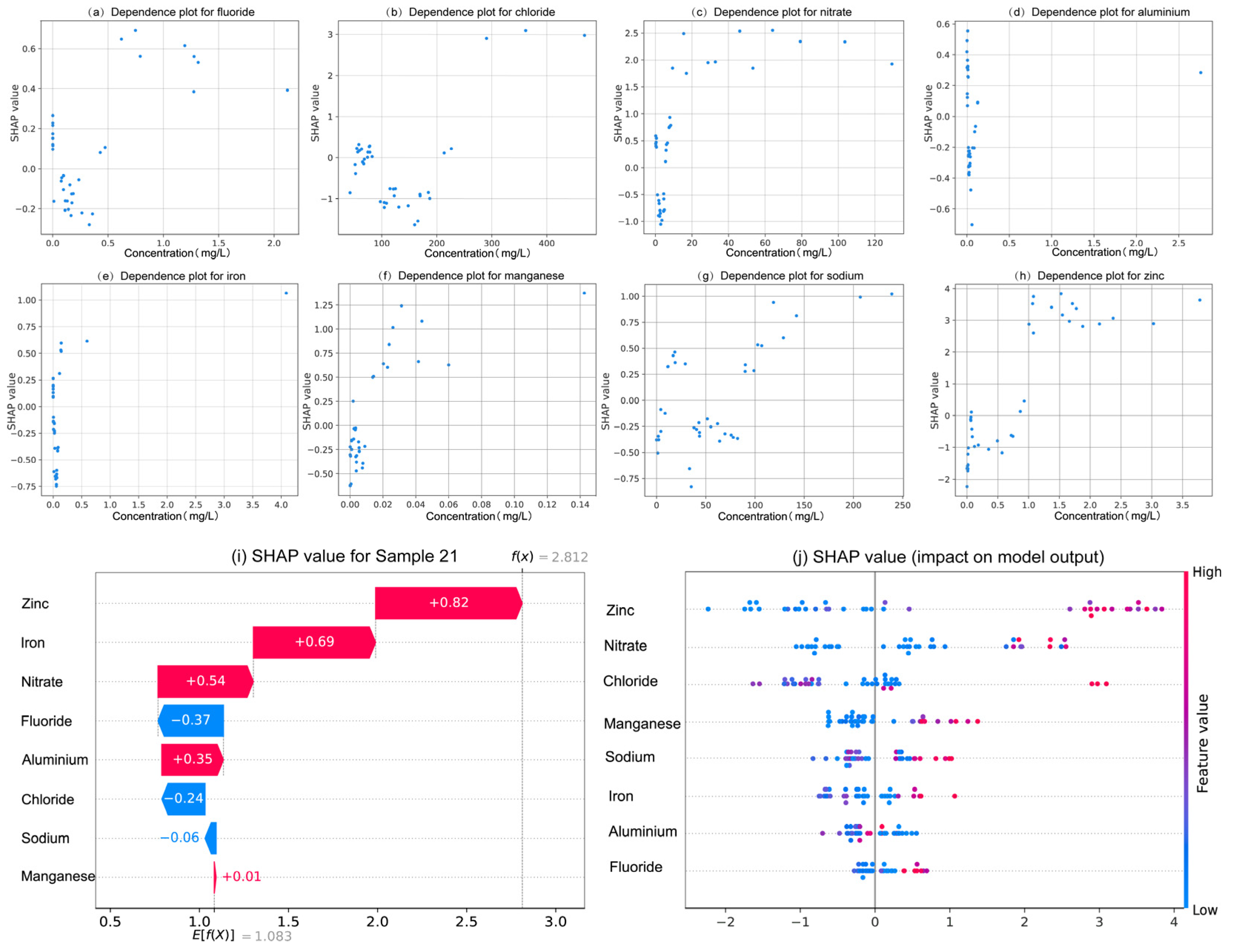
SHAP (Shapley additive explanation) is an ex-post explanation methodology that draws on game theoretic ideas and is able to explain black-box models by calculating the marginal contribution of each feature in the model to measure the magnitude of the influence of each feature [37]. SHAP describes the influence of each feature on the results of the model by means of additivity.

For a single sample x in the black-box model f, the expression for the ex-post explanatory model g is:

$$g\left(x\right)={\varphi }_0+\sum _{i=0}^M{\varphi }_i$$

(7)

where M is the number of features in the black-box model, ${\varphi }_0$ is the average of the predicted values of f with respect to all the samples, and ${\varphi }_i$ is the Shapley value of the ith feature. The ex-post interpretation model g has local accuracy. The predicted value of the ex-post interpretation model g for a single sample is equal to the predicted value of the black-box model for a single sample. Thus, there is the following calculation:

$$f\left(x\right)=g\left(x\right)={\varphi }_0+\sum _{i=0}^M{\varphi }_i$$

(8)

$${\varphi }_i=\sum _{S\subseteq \left\{M\backslash x_i\right\}}{\displaystyle \frac{\left|S\right|!\left(\left|M\right|-\left|S\right|-1\right)!}{\left|M\right|!}}\left\{f\left(x_{S\cup \left\{i\right\}}\right)-f\left(x_S\right)\right\}$$

(9)

where S denotes the feature subset of {M\$x_i$}, and different values represent different feature combinations; $f\left(x_{S\cup \left\{i\right\}}\right) \mathrm{a}\mathrm{n}\mathrm{d} f\left(x_S\right)$ denote the outputs of the model when $x_i$ is modeled and not modeled under the feature combinations, respectively; and ${\displaystyle \frac{\left|S\right|!\left(\left|M\right|-\left|S\right|-1\right)!}{\left|M\right|!}}$ denotes the corresponding probabilities under various combinations of features.

2.5. Human Health Risk Assessment

2.5.1. Deterministic Assessment of Human Health Risks

Human health risk assessment is a quantitative method used to assess the relationship between hazardous substances and human health. Human health risks are evaluated based on methods recommended by the U.S. Environmental Protection Agency (Washington, DC, USA). The potential risks from groundwater are primarily from direct ingestion (drinking) and dermal contact (bathing and swimming). The eight indicators used in this study are all non-carcinogens.

For non-carcinogenic effects of a single contaminant, the groundwater exposure corresponding to drinking was considered and calculated using Equation (10):

$$CDI={\displaystyle \frac{C\times IR\times EF\times ED}{AT\times BW}}$$

(10)

where ADD is the average daily exposure dose of the pollutant, IR is the amount of water consumed per day, C is the concentration of the pollutant in the water body, EF is the frequency of exposure, ED is the duration of exposure, BW is the average body weight, and AT is the average duration of non-carcinogenic effects.

The groundwater exposure corresponding to dermal exposure was considered and calculated using Equation (11):

$$DAD={\displaystyle \frac{K_P\times C\times t_a\times E_V\times SA\times EF\times ED}{AT\times BW}}$$

(11)

where DAD is the average daily absorbed dose of pollutant by skin contact, TC is the duration of exposure, K is the skin permeability coefficient of the hazardous substance, SA is the surface area of exposed skin, and E_V is the average number of daily exposures. See

Table A1. The explanation and values of the parameters in HHR calculation.

Parameters	Explanation	Value	Unit
C	Index concentration	-	mg/L
IR	Ingestion rate	2.2	L/d
SA	Skin area	17,000	cm2
ta	Contact time	0.5	h
KP	Skin permeability coefficient	0.001	cm/h
EF	Exposure frequency	350	d/a
ED	Exposure duration	30	year
EV	Daily exposure frequency of dermal contact event	1	times/d
BW	Body weight	62.2	kg
AT	Average time	ED × 365	d
HQoral	Oral intake hazard quotient	-	-
HQdermal	Dermal intake hazard quotient	-	-

and

Table A2. RfD (mg/kg*d) values of groundwater human health risk assessment mode.

Parameters	RfDoral	RfDdermal
Fluoride	0.04	0.04
Chloride	50	150
Nitrate	1.6	1.6
Aluminum	1	0.2
Iron	0.7	0.14
Manganese	0.024	0.00096
Sodium	100	100
Zinc	0.3	0.06

for relevant parameters.

The human health risk was calculated using Equations (12) and (13):

$$HQ={\displaystyle \frac{ADD}{RfD}}$$

(12)

$$HI={HQ}_{oral}+{HQ}_{dermal}$$

(13)

2.5.2. Source-Specific Human Health Risk Assessment

The receptor model is a mathematical method to analyze the source of pollutants based on environmental monitoring data. By analyzing the concentration characteristics of pollutants, the possible types, quantities, and contribution rates of emission sources can be deduced. Positive definite matrix factorization (PMF) is one of the receptor modeling methods recommended by the U.S. Environmental Protection Agency [38]. Its use of correlation and covariance matrices to simplify high-dimensional variables does not rely on the original spectrum provided by the need for a priori knowledge in the parsing process, and can deal with imprecise data, making it a simple and effective method for pollutant source parsing [39]. Its specific principles are described in Appendix A.

3. Results and Discussion

3.1. Explainable Groundwater Quality Assessment

Machine learning is a technique that enables computer systems to automatically learn and improve models through data training, and it centers on allowing computers to learn patterns from data and make predictions or decisions based on those patterns on new data [40]. This study compares six common algorithms (

Table 2. Comparison of the effect of different algorithms.

Model	Category	Accuracy	Model	Category	Accuracy
KNN	White-box model	0.61	XGBoost	Black-box model	0.97
Logistic regression		0.82	ADaBoost		0.94
Support vector machines		0.65	RNN		0.84

). The black-box models generally outperform the white-box models, which may be due to the fact that black-box models are more complex in principle and are better at learning data laws [18]. Among the black-box models, XGBoost, as an integrated learning algorithm based on decision trees, was applied with superior results and was used for the construction of the XWQI with clearer principles and better internal interpretability compared to ADaboost and RNN [41].

3.1.1. XGBoost Model Validation

AUC-ROC (area under the receiver operating characteristic curve) is an important index for judging the learning performance of a binary classification model, which integrates the model performance under different thresholds. An AUC-ROC value closer to 1 indicates that the model adequately learns the relationship between the data and has a good discriminative ability and robustness [42].

Table 3. Optimized XGBoost hyperparameter values.

Model Hyperparameters	Value
learning_rate	0.12
n_estimators	1000
max_depth	3
min_child_weight	1
gamma	0.4
subsample	0.6
colsample_bytree	0.7
scale_pos_weight	1

demonstrates the best hyperparameter combination after grid search optimization, which has the largest AUC-ROC value (Figure 2).

Table 4. Fold cross-validation results of the XGBoost model.

Iteration	Accuracy	Precision	Recall	F1-Score	AUC
1	94.74%	96.30%	96.30%	96.30%	96.63%
2	97.37%	96.43%	100.00%	98.18%	98.65%
3	97.37%	96.00%	100.00%	97.96%	99.40%
4	97.37%	96.77%	100.00%	98.36%	95.00%
5	94.74%	100.00%	93.10%	96.43%	94.64%

demonstrates all the results in the five-fold cross-validation, with an average precision of 0.971 and an average AUC-ROC of 0.968, which is good for the model.

Grid search is a commonly used hyperparameter tuning method. It traverses all possible hyperparameter combinations by an exhaustive method to find the best performance combination. When using this algorithm, it is necessary to determine the tuned hyperparameters and evaluation indicators, then evaluate the performance of each parameter combination through cross-validation to reduce the risk of overfitting and select the optimal parameter combination according to the evaluation indicators. Finally, the best parameter combination is used to verify the performance of the model on the validation set or test set to ensure its generalization ability.

The loss curve is a visualization tool commonly used in machine learning and deep learning to monitor the change in model performance during training [43]. For classification tasks, the commonly used loss function is log loss. In Figure A1, the training set loss decreases with the increase in training rounds, and the validation set loss also decreases with the increase in training rounds and tends to stabilize, indicating that the model is stable and that its performance improves with each iteration, and that the overall convergence does not have overfitting or underfitting phenomena. Based on the assessment index, the performance of XGBoost is excellent and robust, and due to the internal structure of XGBoost, its application is internally explainable, i.e., the computational results of the verified XGBoost are mathematically explainable and reliable.

3.1.2. Groundwater Quality Assessment Results and Analysis

On the basis of the existing water quality dataset, the XWQI model is constructed by selecting the indexes that exceed the standard. In this study, fluoride, chloride, nitrate, aluminum, iron, manganese, sodium, and zinc were selected to construct a water quality evaluation model (

Table 5. Statistical results of chemical composition of groundwater in the research area.

Indicators	Max (mg/L)	Median (mg/L)	Min (mg/L)	Average (mg/L)	SD	CV
Fluoride	2.121	0.135	0.001	0.272	0.384	1.408
Chloride	975.266	114.533	14.61	177.149	165.624	0.935
Nitrate	178.485	3.394	0.001	12.395	28.045	2.263
Aluminum	5.149	0.019	0.0001	0.105	0.47	4.495
Iron	8.001	0.024	0.0001	0.171	0.71	4.149
Manganese	0.81	0.004	0.0001	0.024	0.072	3.012
Sodium	508.237	45.103	0.0001	72.924	81.671	1.12
Zinc	5.845	0.351	0.0001	0.882	1.113	1.262

).

In determining the weights of the metrics, the dataset was divided into two parts: the training set (80%) and the test set (20%). The training set is used for the XGBoost algorithm to learn the objective connection between the data, and the test set is used to verify the learning effect. The validation shows that the results of XGBoost’s weight calculation were highly reliable and could be applied to the process of groundwater quality condition assessment. Figure 3 shows the results of multiple calculations of the weights of the eight water quality indicators. There were acceptable fluctuations in the results of multiple calculations, and the overall trend was consistent, with Zn, NO₃⁻, Cl⁻, and Na representing the four items with the highest average weights. Figure 4 demonstrates the spatial distribution of the exceedance status of the eight indicators. Spatially, these four indicators are also the four items with the most serious degree of exceedance, proving that the weight values obtained by XGBoost are consistent with the actual macro conditions.

The overall quality of groundwater in the study area was found to be suitable for drinking. The WQI was calculated to be between 4.32 and 445.63, with a mean value of 66.27 and a median value of 51.79, and the assessment criteria are presented in

Table 6. Classification schemes of the XWQI models.

Score	Classification	Instruction
<50	Excellent	The water quality is excellent and can be used for various use types.
50~100	Good	The content of chemical components in groundwater is low, which is suitable for various uses.
101~200	Poor	The chemical content is at a medium level, and after treatment it may be used as drinking water.
201~300	Very poor	The water is suitable for agriculture and some industry
>300	Unfit	The content of chemical components is high, which is unsuitable for drinking.

[43]. Compared with other classification criteria, this classification scheme does not set an upper limit. This shows that the classification scheme can compare the unqualified water quality and better reflect the water quality status. A total of 49% of the groundwater samples were of excellent quality, 33% of the samples were of good quality, and 18% of the samples were contaminated and unsuitable for drinking. Good-quality groundwater was concentrated in the southwestern, central, and southeastern parts of the study area; groundwater with contamination was concentrated in the northern and southern parts of the area (Figure 4). The four indicators with high weighted values had a wide range of exceedances in the north and south of the study area.

The results of the XWQI assessment show that the spatial distribution of high-quality groundwater is basically consistent with the distribution of the population in the study area, indicating that the local water quality management authorities have implemented efficient water quality maintenance measures to ensure the safety of people’s water use. Due to the high population density in some areas, high-frequency anthropogenic activities still have an impact on the quality of groundwater, and there were exceedances of Cl⁻ and Na in a small number of points. The presence of industrial enterprises such as metal processing, livestock farms, and leather processing and manufacturing, as well as pollution sources such as petrol stations and farmlands, in the study area may be one of the reasons for the deterioration in groundwater quality.

3.1.3. Explaining Groundwater Quality with Key Characteristic Variables

In this study, the SHAP tool was used to perform explainable analysis of groundwater quality conditions using characteristic variables globally and locally. Each of the eight indicators contributed differently to the water quality condition judgment (Table A2). Overall, zinc had an extremely strong influence on XGBoost’s decision-making, as did chloride and nitrate. To assess the similarity and stability of the model results, Pearson correlation coefficients were calculated using Python 3.12 (Figure 5). The results of the five iterations of calculations show that the correlation between the weights and the contribution values were all strong, with a positive correlation except for the weights of the fourth iteration. The correlation coefficient between weights and contribution values was calculated for the results of each iteration, and the mean value was 0.836. Figure 6a–h shows the dependency plots for each water quality indicator, indicating the relationship between the indicator concentration and its effect on the model predictions. The SHAP values of all the indicators showed an increasing trend with increasing concentration. The SHAP values for zinc, chloride, and nitrate were much higher than the other indicators, indicating a great influence on the judgment of water quality conditions.

The third iteration of the results was chosen for analysis in this study, and its accuracy was 97.37%, with one sample misjudged. This sample passed all the indicators (

Table A3. The indicator contribution value obtained by XGBoost through multiple iterations.

Indicators	Iteration 1	Iteration 2	Iteration 3	Iteration 4	Iteration 5
Fluoride	0.304	0.456	0.231	0.338	0.431
Chloride	0.969	1.000	0.784	1.134	0.878
Nitrate	0.937	0.922	1.076	1.044	0.976
Aluminum	0.189	0.238	0.284	0.237	0.230
Iron	0.340	0.532	0.383	0.319	0.255
Manganese	0.377	0.400	0.463	0.473	0.551
Sodium	0.256	0.380	0.422	0.338	0.206
Zinc	1.858	1.878	1.823	2.261	1.897

). SHAP analysis showed that XGBoost started with an $E\left[f\right(x\left)\right]$ of 1.083, and after the combined effect of different indicators, $f\left(x\right)$ was 2.812, which was categorized as failing (Figure 6i,j). F⁻, Cl⁻, and Na had a positive effect on the results, which contributed to the categorization of XGBoost as passing. When the values of F⁻, Cl⁻, and Na concentrations are much lower than the standard values, the water quality is much better and the tendency to pass is extremely high. The remaining five metrics had a positive effect on the results, with the ratio of concentration values to standard values increasing as the contribution increased, prompting a bias toward failing the final results. The concentration of zinc was 0.9688 mg/L, not exceeding the standard of 1 mg/L but extremely close, and it also had the highest ratio of the five indicators and the highest positive contribution rate of 0.82. The negative contribution rate of Fe was 0.69, also due to the high ratio. The presence of a garage and a machine shop in the vicinity of the site may have contributed to the elevated concentrations of Fe and Zn. The reason for misclassification of the site can be attributed to the fact that the concentrations of Zn and Fe were close to the standard values, which were not exceeded but posed a high risk of contamination, and it was an acceptable amount of error.

The study compared and analyzed the SHAP results of 38 sets of data in the test set (Figure A3, Figure A4 and Figure A5). The four indicators of zinc, chloride, nitrate, and manganese had a strong impact on water quality, and the absolute value of global contribution was high although the intensity and direction of the impact varied at different points. This indicates that although the indicators influence water quality in different directions, they have a key role in determining water quality and are identified as key variables affecting groundwater quality in the study area.

3.2. Sources of Groundwater Contamination

3.2.1. Source Identification Results of Groundwater Contamination Based on PMF

To further explore the contribution of the eight indicators to water quality status and human health risk, PMF was used to analyze the sources of the eight indicators in the study area. The dimensionality was reduced by principal component analysis, and four sources were finally set. The categories of the eight indicators were set as strong. Figure 7 demonstrates the PMF model construction results and the identification indicator of the four factors.

The main loads of Factor 1 were fluoride (95.8%) and nitrate (81.7%). Large areas of agricultural cropland and residential villages exist in the study area, and their distribution intersects with the spatial distribution of fluoride ions and nitrate. Fertilizers and pesticides containing fluoride and nitrogen are commonly used by farmers in agricultural production. Residues of these chemicals in the soil can enter water bodies with rainwater or irrigation water, leading to simultaneous contamination of fluoride ions and nitrates. Factor 1 was therefore categorized as an agricultural source.

The main loading for Factor 2 was zinc (96.7%) and nitrate (18.3%), with low loading. Zinc is a common pollutant and is commonly found in industrial establishments involved in metal processing and electroplating, while some nitrates are emitted due to the presence of chemicals during processing. In addition, wastewater from leather processing may also be converted to nitrate during treatment and also contain heavy metals such as zinc [44]. There are six leather processing plants and two electroplating enterprises in the study area, and there may be zinc-containing wastewater discharge. Therefore, Factor 2 was classified as metal processing and electroplating.

The main loadings of Factor 3 are aluminum (96%), iron (96.8%), and manganese (69.6%), which are common indicators of pollution from industrial emissions. There are eight non-ferrous metal processing industrial enterprises in the study area, and there are iron and manganese mining projects, as well as some chemical-related manufacturing industries, which emit aluminum, iron, and manganese pollution [45]. Therefore, Factor 3 was categorized as an industrial source and differed significantly from the industrial sources of Factor 2.

It should be noted that, compared with Factor 2, although both can be classified as industrial pollution sources, there are significant differences in the main load indicators, and there is no common load indicator. The main load indexes of Factor 2 and Factor 3 point to metal processing and electroplating, and non-ferrous metal smelting and mining, respectively. Therefore, Factor 2 and Factor 3 represent different pollution sources.

The main loads for Factor 4 were chloride (91.3%) and sodium (90.8%) ions. Earlier studies have shown that on the one hand, the submerged layer in the study area is loose, with good runoff conditions, and that the rise in the groundwater level leads to the dissolution of salt minerals in the rock strata, resulting in an increase in the concentration of chloride and sodium ions. With the implementation of the groundwater recharge project, the rise in water level greatly shortens the time for salt minerals to enter the aquifer. The increase in the concentration of chloride and sodium ions is mainly due to the dissolution and filtration of the formation during the groundwater level rise, so Factor 4 was categorized as a natural source.

3.2.2. Uncertainty Analysis of Pollution Source Apportionment

When the PMF model is used to analyze the source of groundwater pollution in the Manas River Basin, due to the small influence of the non-identified elements of each pollution source on the operation of the PMF model, only the main load indicators of each pollution source are analyzed for uncertainty. In this study, three uncertainty calculation methods, BS, DISP and BS-DISP, were used to evaluate the overall uncertainty of the analytical calculation of groundwater pollution sources. The uncertainty intervals of the three error estimation methods are shown in

Table 7. The uncertainty interval of three error estimation methods for the identification of elements of pollution sources.

Source	Indicator	Basal Value	Uncertainty Interval
			BS	DISP	BS-DISP
Factor1	Fluoride	0.07386	[0.002973, 0.15235]	[0.071163, 0.076751]	[0, 0.1596]
	Nitrate	0.016645	[0, 0.05329]	[0.015002, 0.018211]	[0, 0.05635]
Factor 2	Zinc	0.12616	[0.067492, 0.13651]	[0.12196, 0.13137]	[0, 0.139]
Factor 3	Aluminium	0.017406	[0.016025, 0.01784]	[0.016401, 0.018336]	[0, 0.01866]
	Iron	0.016126	[0.014764, 0.018686]	[0.015146, 0.017005]	[0, 0.01971]
	Manganese	0.0062802	[0.00545, 0.0075]	[0.00588, 0.00664]	[0, 0.007843]
Factor 4	Chloride	0.10574	[0.03795, 0.12522]	[0.10205, 0.11236]	[0, 0.1416]
	Sodium	0.11928	[0, 0.11973]	[0.11543, 0.12621]	[0, 0.1219]

. The specific principles are described in the Appendix A.

Except for the sodium in Factor 4, the BS estimation range and DISP estimation range of all other indicators were smaller than the BS-DISP estimation range, and the DISP estimation range was the smallest, indicating that the rotation uncertainty generated by factorization is small during the operation of the PMF model. The estimation range of BS-DISP shows that the estimation range of chloride and sodium in Factor 4 was large, and the estimation range of other factors and indicators was smaller than the estimation range of chloride and sodium in Factor 4, indicating that the source apportionment results of Factor 1, Factor 2, and Factor 3 are more stable than the source apportionment results of Factor 4. On the whole, the results of groundwater pollution source analysis in the Manas River Basin are acceptable based on combining the results of uncertainty interval analysis and interval ratio analysis.

3.2.3. Source Identification Results Based on SHAP Model

From the results of source type identification, it can be seen that there are four main sources of groundwater contamination in the study area: agricultural activities, metal processing, metal smelting and mining, and natural sources. SHAP identified the key variables for water quality as zinc, chloride, nitrate, and manganese, and a comparison with the results of the PMF model construction revealed that zinc was the identifying element in the metal processing source (Factor 2), with a relative contribution of 78.3%, and chloride was the natural source (Factor 4), with a relative contribution of 83.8% together with sodium. Nitrate was an identifier in the agricultural source (Factor 1), with a relative contribution of 81.7%, and manganese was an identifier in the industrial source (Factor 3), with a relative contribution of 69.9%. The key variables identified by SHAP have strong similarities with the results obtained from the pollution sources that were modelled by PMF. The four key variables correspond to the four types of pollution sources and are all major loading elements.

3.3. Results and Analysis of Human Health Risk Assessment from Specific Sources

3.3.1. Health Risk Assessment Results and Analysis

According to the U.S. Environmental Protection Agency’s definition of health risk, there is an unacceptable human health risk when HI is greater than or equal to 1. The spatial distribution of human health risks of eight indicators in groundwater is shown in Figure 8. As the most serious indicator of pollution status, zinc poses the greatest risk to human health, which is also reflected in the spatial distribution of health risks. The central and northern parts of the study area are facing serious health risks from zinc. The risk caused by chloride is mainly distributed in the north and south of the study area. The southern part of the study area is mainly industrial metal smelting and processing enterprises, with a high health risk from aluminum, iron, and manganese. The average value of HI was 2.55, and the median was 1.98, both of which were greater than 1. This indicates that the overall non-carcinogenic risk of groundwater is high. About 74.8% of the sample risk value was higher than the standard risk value. The non-carcinogenic risk of direct intake was much higher than that of skin contact, indicating that groundwater is more likely to affect human health, such as excessive drinking or cooking. Except for fluoride, the maximum values of the other indicators were greater than 1, all of which had non-carcinogenic risks. The average risk of iron and chloride was greater than 1, indicating that the non-carcinogenic risk of these two indicators is much higher than other indicators, which has a greater impact on human health. The maximum values of iron and zinc were 19.237 and 7.02, respectively, which are much higher than 1, reflecting the extremely high level of space pollution, and the health of residents in the surrounding areas was more susceptible to zinc and iron.

3.3.2. Validation and Quantification of the Effects of Key Variables on Human Health

The relative contribution of different sources to non-carcinogenic risk was calculated. The average value from high to low was 57.22% for metal processing, 24.98% for metal smelting and mining, 17.68% for agricultural activities, and 0.13% for natural sources. Among these, metal processing and metal smelting mining are the main sources of non-carcinogenic risks in the study area. Chlorine and sodium in groundwater usually exist in the form of ions, and humans have good tolerance to them. The human body can ingest 5–9 g of chloride ions per day, so the non-carcinogenic risk of natural sources is the lowest. The average relative contribution of metal processing was as high as 57.22%, and PMF showed that zinc comprised the main load. As one of the indicators of groundwater pollutants, the human tolerance of zinc leads to a lower RfD value, which increases the contribution of zinc to non-carcinogenic risk.

Explainable machine learning analysis showed that zinc, chloride, nitrate, and manganese were the four key indicators. Zinc was the index with the highest rate of contribution to human health risk (34.46%), the highest HI was 7.02, and the over-standard rate was 41.2%, which had a significant negative impact on human health. The relative contribution of chloride was 27.34%, and the maximum HI was 2.35. Although the over-standard rate was not high (about 9%), the average value was 0.426, which had a significant impact on the comprehensive results. The relative contribution rate of nitrate was 12.2%, with an average of 0.297. Compared with zinc and chloride, nitrate had less impact on human health. The relative contribution of manganese was low (3.5%), only higher than that of fluorine and aluminum. The relative contribution rate of the four key indicators that can explain machine learning recognition of human health risks was about 77.5%, which was the main factor affecting human health.

4. Conclusions

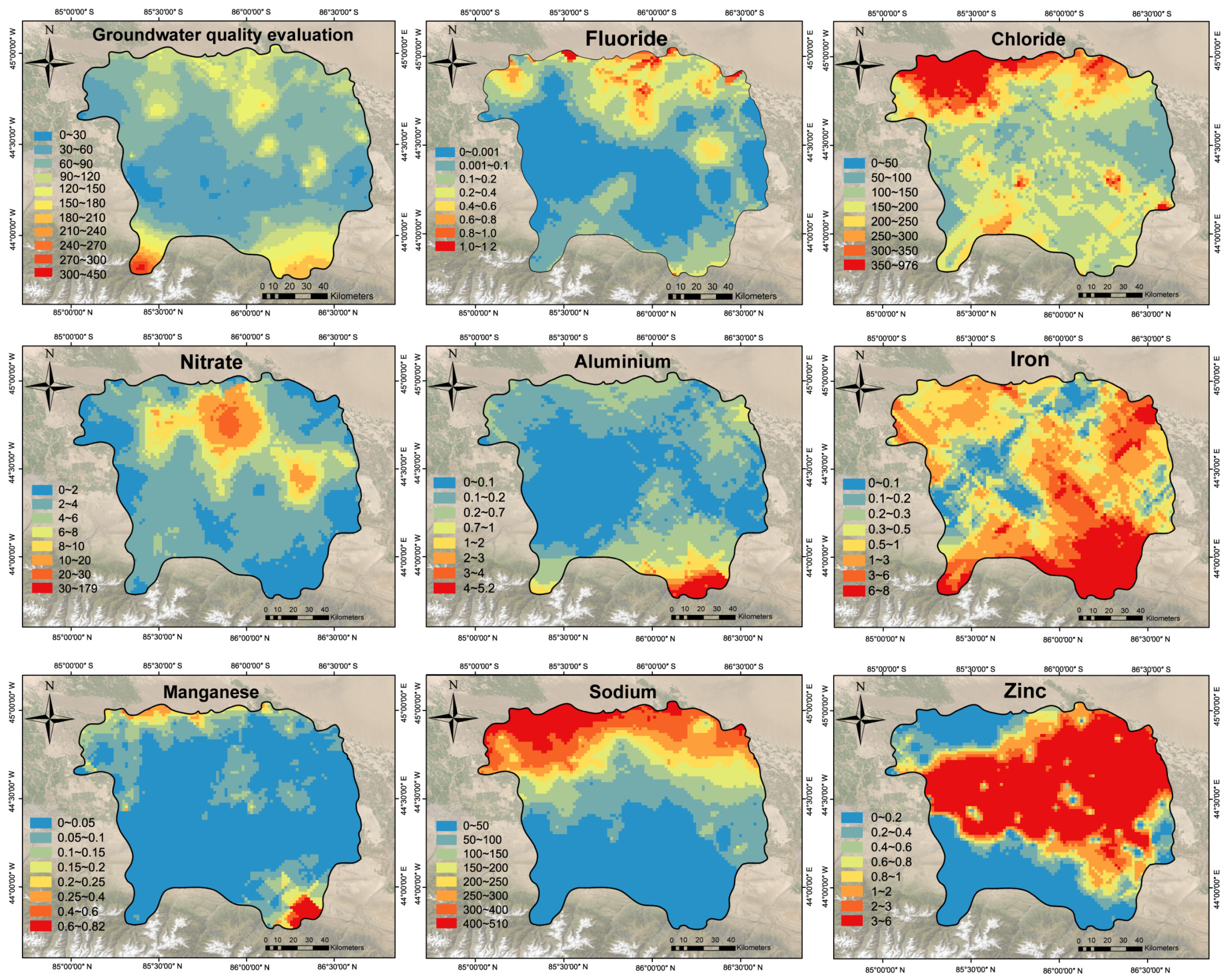
The main goal of this study is to determine the key indicators affecting water quality through data analysis, to clarify the sources of human health risks, and to provide reference for water quality management departments. The XWQI was constructed by interpretable machine learning, and eight indicators were used to evaluate the groundwater quality in the study area. The human health risks of each indicator were calculated, and the pollution sources and health risk sources were identified by PMF. The overall groundwater situation in the study area is excellent. A total of 49% of the samples can be directly used as drinking water sources, 33% of the samples can also be drunk after simple treatment, and 18% of the samples are polluted and not suitable for drinking. The XWQI showed excellent performance, assigned weights to water quality indicators, and further confirmed zinc, chloride, and nitric acid as key pollution indicators through SHAP interpretability analysis. Among them, the contribution of zinc was the highest (0.82), and its concentration did not exceeded but was close to the critical value (0.968 mg/L), revealing the early warning value of “sub-threshold pollution risk”. The misjudgment case of the model further confirms the sensitivity characteristics of the water pollution boundary, and proves the rationality and reliability of XGBoost in the process of water quality evaluation. The PMF model analysis showed that the sources of pollution were agricultural activities, metal processing, metal smelting and mining, and natural sources. Among these, industrial pollution sources accounted for 82.2%, indicating that there is serious industrial pollution in the study area and that it should have a higher priority in governance. In addition, it was indicated that metal processing (57.22%) and smelting and mining (24.98%) were the two major sources of human health risks based on water quality.

This study greatly improves the credibility of the application of machine learning in water quality assessment. The inclusion of explainable analysis reveals the basis of judgment of black-box models, helps researchers to identify key indicators and quantify their influence, and improves the credibility of machine learning. The PMF intervention helped to identify groundwater pollution sources and human health risk sources, and successfully validated the correctness of the SHAP algorithm in identifying key water quality indicators and providing a reference for water quality management authorities.

References

1. Liu, R.; Xie, X.; Hou, Q.; Han, D.; Song, J.; Huang, G. Spatial Distribution, Sources, and Human Health Risk Assessment of Elevated Nitrate Levels in Groundwater of an Agriculture-Dominant Coastal Area in Hainan Island, China. J. Hydrol. 2024, 634, 131088. [Google Scholar] [CrossRef]
2. Abascal, E.; Gómez-Coma, L.; Ortiz, I.; Ortiz, A. Global Diagnosis of Nitrate Pollution in Groundwater and Review of Removal Technologies. Sci. Total Environ. 2022, 810, 152233. [Google Scholar] [CrossRef] [PubMed]
3. Cao, X.; Shi, Y.; He, W.; An, T.; Chen, X.; Zhang, Z.; Liu, F.; Zhao, Y.; Zhou, P.; Chen, C.; et al. Impacts of Anthropogenic Groundwater Recharge (AGR) on Nitrate Dynamics in a Phreatic Aquifer Revealed by Hydrochemical and Isotopic Technologies. Sci. Total Environ. 2022, 839, 156187. [Google Scholar] [CrossRef]
4. Wang, Z.-J.; Yue, F.-J.; Lu, J.; Wang, Y.-C.; Qin, C.-Q.; Ding, H.; Xue, L.-L.; Li, S.-L. New Insight into the Response and Transport of Nitrate in Karst Groundwater to Rainfall Events. Sci. Total Environ. 2022, 818, 151727. [Google Scholar] [CrossRef] [PubMed]
5. Gwira, H.A.; Osae, R.; Abasiya, C.; Peasah, M.Y.; Owusu, F.; Loh, S.K.; Kojo, A.; Aidoo, P.; Agyare, E.A. Hydrogeochemistry and Human Health Risk Assessment of Heavy Metal Pollution of Groundwater in Tarkwa, a Mining Community in Ghana. Environ. Adv. 2024, 17, 100565. [Google Scholar] [CrossRef]
6. Javed, S.; Ali, A.; Ullah, S. Spatial Assessment of Water Quality Parameters in Jhelum City (Pakistan). Environ. Monit. Assess. 2017, 189, 119. [Google Scholar] [CrossRef] [PubMed]
7. Sotomayor, G.; Hampel, H.; Vázquez, R.F. Water Quality Assessment with Emphasis in Parameter Optimisation Using Pattern Recognition Methods and Genetic Algorithm. Water Res. 2018, 130, 353–362. [Google Scholar] [CrossRef]
8. Lumb, A.; Sharma, T.C.; Bibeault, J.-F. A Review of Genesis and Evolution of Water Quality Index (WQI) and Some Future Directions. Water Qual. Expo. Health 2011, 3, 11–24. [Google Scholar] [CrossRef]
9. Sutadian, A.D.; Muttil, N.; Yilmaz, A.G.; Perera, B.J.C. Development of River Water Quality Indices—A Review. Environ. Monit. Assess. 2016, 188, 58. [Google Scholar] [CrossRef]
10. Ewaid, S.H.; Abed, S.A.; Kadhum, S.A. Predicting the Tigris River Water Quality within Baghdad, Iraq by Using Water Quality Index and Regression Analysis. Environ. Technol. Innov. 2018, 11, 390–398. [Google Scholar] [CrossRef]
11. Feng, T.; Wang, C.; Hou, J.; Wang, P.; Liu, Y.; Dai, Q.; Yang, Y.; You, G. Effect of Inter-Basin Water Transfer on Water Quality in an Urban Lake: A Combined Water Quality Index Algorithm and Biophysical Modelling Approach. Ecol. Indic. 2018, 92, 61–71. [Google Scholar] [CrossRef]
12. Wu, Y.; Chen, J. Investigating the Effects of Point Source and Nonpoint Source Pollution on the Water Quality of the East River (Dongjiang) in South China. Ecol. Indic. 2013, 32, 294–304. [Google Scholar] [CrossRef]
13. Das, A.K.; Das, S.; Ghosh, A. Ensemble Feature Selection Using Bi-Objective Genetic Algorithm. Knowl.-Based Syst. 2017, 123, 116–127. [Google Scholar] [CrossRef]
14. Momenzadeh, M.; Sehhati, M.; Rabbani, H. A Novel Feature Selection Method for Microarray Data Classification Based on Hidden Markov Model. J. Biomed. Inform. 2019, 95, 103213. [Google Scholar] [CrossRef] [PubMed]
15. Uddin, M.G.; Imran, M.H.; Sajib, A.M.; Hasan, M.A.; Diganta, M.T.M.; Dabrowski, T.; Olbert, A.I.; Moniruzzaman, M. Assessment of Human Health Risk from Potentially Toxic Elements and Predicting Groundwater Contamination Using Machine Learning Approaches. J. Contam. Hydrol. 2024, 261, 104307. [Google Scholar] [CrossRef]
16. Liu, C.; Xu, J.; Li, X.; Yu, Z.; Wu, J. Water Resource Forecasting with Machine Learning and Deep Learning: A Scientometric Analysis. Artif. Intell. Geosci. 2024, 5, 100084. [Google Scholar] [CrossRef]
17. Vachon, J.; Kerckhoffs, J.; Buteau, S.; Smargiassi, A. Do Machine Learning Methods Improve Prediction of Ambient Air Pollutants with High Spatial Contrast? A Systematic Review. Environ. Res. 2024, 262, 119751. [Google Scholar] [CrossRef]
18. Hakkoum, H.; Idri, A.; Abnane, I. Global and Local Interpretability Techniques of Supervised Machine Learning Black Box Models for Numerical Medical Data. Eng. Appl. Artif. Intell. 2024, 131, 107829. [Google Scholar] [CrossRef]
19. Adilkhanova, I.; Ngarambe, J.; Yun, G.Y. Recent Advances in Black Box and White-Box Models for Urban Heat Island Prediction: Implications of Fusing the Two Methods. Renew. Sustain. Energy Rev. 2022, 165, 112520. [Google Scholar] [CrossRef]
20. Bai, F.; Gong, X.-M.; Li, H.-W.; Guo, H.-B.; Tao, W.-Q. An Improved Black Box Model and the Details of Its Numerical Treatments for Rack in Data Center Simulation. Int. Commun. Heat Mass Transf. 2024, 158, 107916. [Google Scholar] [CrossRef]
21. Lee, H.; Park, S.; V-Minh Nguyen, H.; Shin, H.-S. Proposal for a New Customization Process for a Data-Based Water Quality Index Using a Random Forest Approach. Environ. Pollut. 2023, 323, 121222. [Google Scholar] [CrossRef] [PubMed]
22. Lap, B.Q.; Phan, T.-T.-H.; Nguyen, H.D.; Quang, L.X.; Hang, P.T.; Phi, N.Q.; Hoang, V.T.; Linh, P.G.; Hang, B.T.T. Predicting Water Quality Index (WQI) by Feature Selection and Machine Learning: A Case Study of An Kim Hai Irrigation System. Ecol. Inform. 2023, 74, 101991. [Google Scholar] [CrossRef]
23. Liao, W.; Fang, J.; Ye, L.; Bak-Jensen, B.; Yang, Z.; Porte-Agel, F. Can We Trust Explainable Artificial Intelligence in Wind Power Forecasting? Appl. Energy 2024, 376, 124273. [Google Scholar] [CrossRef]
24. Miller, T. Explanation in Artificial Intelligence: Insights from the Social Sciences. Artif. Intell. 2019, 267, 1–38. [Google Scholar] [CrossRef]
25. Razavi-Termeh, S.V.; Sadeghi-Niaraki, A.; Yao, X.A.; Naqvi, R.A.; Choi, S.-M. Assessment of Noise Pollution-Prone Areas Using an Explainable Geospatial Artificial Intelligence Approach. J. Environ. Manag. 2024, 370, 122361. [Google Scholar] [CrossRef]
26. Jeong, H.; Abbas, A.; Kim, H.G.; Van Hoan, H.; Van Tuan, P.; Long, P.T.; Lee, E.; Cho, K.H. Spatial Prediction of Groundwater Salinity in Multiple Aquifers of the Mekong Delta Region Using Explainable Machine Learning Models. Water Res. 2024, 266, 122404. [Google Scholar] [CrossRef]
27. Kavcar, P.; Sofuoglu, A.; Sofuoglu, S.C. A Health Risk Assessment for Exposure to Trace Metals via Drinking Water Ingestion Pathway. Int. J. Hyg. Environ. Health 2009, 212, 216–227. [Google Scholar] [CrossRef] [PubMed]
28. Zambelli, B.; Uversky, V.N.; Ciurli, S. Nickel Impact on Human Health: An Intrinsic Disorder Perspective. Biochim. Biophys. Acta Proteins Proteom. 2016, 1864, 1714–1731. [Google Scholar] [CrossRef]
29. Biswas, T.; Pal, S.C.; Saha, A.; Ruidas, D.; Islam, A.R.M.; Shit, M. Hydro-Chemical Assessment of Groundwater Pollutant and Corresponding Health Risk in the Ganges Delta, Indo-Bangladesh Region. J. Clean. Prod. 2023, 382, 135229. [Google Scholar] [CrossRef]
30. Zhang, M.; Wang, L.; Zhao, Q.; Wang, J.; Sun, Y. Hydrogeochemical and Anthropogenic Controls on Quality and Quantitative Source-Specific Risks of Groundwater in a Resource-Based Area with Intensive Industrial and Agricultural Activities. J. Clean. Prod. 2024, 440, 140911. [Google Scholar] [CrossRef]
31. Zhou, Y.; Tu, Z.; Zhou, J.; Han, S.; Sun, Y.; Liu, X.; Liu, J.; Liu, J. Distribution, Dynamic and Influence Factors of Groundwater Arsenic in the Manas River Basin in Xinjiang, P.R.China. Appl. Geochem. 2022, 146, 105441. [Google Scholar] [CrossRef]
32. Xu, Z.; Fan, W.; Wei, H.; Zhang, P.; Ren, J.; Gao, Z.; Ulgiati, S.; Kong, W.; Dong, X. Evaluation and Simulation of the Impact of Land Use Change on Ecosystem Services Based on a Carbon Flow Model: A Case Study of the Manas River Basin of Xinjiang, China. Sci. Total Environ. 2019, 652, 117–133. [Google Scholar] [CrossRef] [PubMed]
33. Yang, G.; Tian, L.; Li, X.; He, X.; Gao, Y.; Li, F.; Xue, L.; Li, P. Numerical Assessment of the Effect of Water-Saving Irrigation on the Water Cycle at the Manas River Basin Oasis, China. Sci. Total Environ. 2020, 707, 135587. [Google Scholar] [CrossRef]
34. Ejaz, U.; Khan, S.M.; Jehangir, S.; Ahmad, Z.; Abdullah, A.; Iqbal, M.; Khalid, N.; Nazir, A.; Svenning, J.-C. Monitoring the Industrial Waste Polluted Stream—Integrated Analytics and Machine Learning for Water Quality Index Assessment. J. Clean. Prod. 2024, 450, 141877. [Google Scholar] [CrossRef]
35. Maharana, K.; Mondal, S.; Nemade, B. A Review: Data Pre-Processing and Data Augmentation Techniques. Glob. Transit. Proc. 2022, 3, 91–99. [Google Scholar] [CrossRef]
36. Xu, T.; Tian, A.; Gao, J.; Yan, H.; Liu, C. Analysis of the Spatial Heterogeneity of Glacier Melting in Tibet Autonomous Region and Its Influential Factors Using the K-Means and XGBoost-SHAP Algorithms. Environ. Model. Softw. 2024, 182, 106194. [Google Scholar] [CrossRef]
37. Gupta, A.; Gowda, S.; Tiwari, A.; Gupta, A.K. XGBoost-SHAP Framework for Asphalt Pavement Condition Evaluation. Constr. Build. Mater. 2024, 426, 136182. [Google Scholar] [CrossRef]
38. Shi, B.; Yang, X.; Liang, T.; Liu, S.; Yan, X.; Li, J.; Liu, Z. Source Apportionment of Soil PTE in a Northern Industrial County Using PMF Model: Partitioning Strategies and Uncertainty Analysis. Environ. Res. 2024, 252, 118855. [Google Scholar] [CrossRef]
39. Frischmon, C.; Hannigan, M. VOC Source Apportionment: How Monitoring Characteristics Influence Positive Matrix Factorization (PMF) Solutions. Atmos. Environ. X 2024, 21, 100230. [Google Scholar] [CrossRef] [PubMed]
40. Xu, J. Comparing Multi-Class Classifier Performance by Multi-Class ROC Analysis: A Nonparametric Approach. Neurocomputing 2024, 583, 127520. [Google Scholar] [CrossRef]
41. Niazkar, M.; Menapace, A.; Brentan, B.; Piraei, R.; Jimenez, D.; Dhawan, P.; Righetti, M. Applications of XGBoost in Water Resources Engineering: A Systematic Literature Review (Dec 2018–May 2023). Environ. Model. Softw. 2024, 174, 105971. [Google Scholar] [CrossRef]
42. Uddin, M.G.; Nash, S.; Rahman, A.; Olbert, A.I. A Comprehensive Method for Improvement of Water Quality Index (WQI) Models for Coastal Water Quality Assessment. Water Res. 2022, 219, 118532. [Google Scholar] [CrossRef] [PubMed]
43. Krishnamoorthy, N.; Thirumalai, R.; Lenin Sundar, M.; Anusuya, M.; Manoj Kumar, P.; Hemalatha, E.; Mohan Prasad, M.; Munjal, N. Assessment of Underground Water Quality and Water Quality Index across the Noyyal River Basin of Tirupur District in South India. Urban Clim. 2023, 49, 101436. [Google Scholar] [CrossRef]
44. Singh, B.J.; Chakraborty, A.; Sehgal, R. A Systematic Review of Industrial Wastewater Management: Evaluating Challenges and Enablers. J. Environ. Manag. 2023, 348, 119230. [Google Scholar] [CrossRef]
45. Luo, M.; Zhang, Y.; Li, H.; Hu, W.; Xiao, K.; Yu, S.; Zheng, C.; Wang, X. Pollution Assessment and Sources of Dissolved Heavy Metals in Coastal Water of a Highly Urbanized Coastal Area: The Role of Groundwater Discharge. Sci. Total Environ. 2022, 807, 151070. [Google Scholar] [CrossRef]
Figure 1. Geographic location of the Manas River and distribution of sampling sites.
Water 17 00905 g001
Figure 2. AUC-ROC image of each iteration in the 5-fold crossover operation.
Water 17 00905 g002
Figure 3. The indicator weight value obtained by XGBoost through multiple iterations.
Water 17 00905 g003
Figure 4. Spatial distribution of groundwater quality evaluation results and concentration values of eight water quality indicators.
Water 17 00905 g004
Figure 5. The correlation coefficient of the index weight and contribution value. (a) The correlation between the weight values obtained by each iteration; (b) the correlation between the contribution values obtained.
Water 17 00905 g005
Figure 6. Contributions calculated by the SHAP tool. (ah) The relationship between SHAP values and concentrations for each indicator in the dataset in the form of a dependency plot; (i) the SHAP analysis plot for Sample 21; (j) the overall SHAP calculation results for the test dataset.
Water 17 00905 g006
Figure 7. Results of PMF modeling and identification indicators for each pollution source.
Water 17 00905 g007
Figure 8. Spatial distribution of the results of the human health risk assessment.
Water 17 00905 g008