Dynamic Changes in Both Summer Potential Evapotranspiration and Its Driving Factors in the Huai River Basin, China

Abstract

Potential evapotranspiration (ETp) is an important component of the water and energy cycle. This study investigated the changing patterns of both summer ETp and its drivers in the Huai River Basin for the first time using the newly proposed anomaly contribution analysis method, as summer is usually the peak period of ETp but little has been done to study it specifically. The anomaly contribution analysis method is able to calculate the contribution rates of climate factors to summer ETp for every year, which helps to reveal the dynamic changes in the contribution of climate factors to summer ETp. The results show that the evaporation paradox is not accurate for the basin since summer ETp declines significantly while the trend of summer Tm is insignificant. Influenced by the abrupt changes in summer Sh and Ws, summer ETp underwent a mutation around the 1970s and 1980s. Sensitivity analysis and contribution analysis show that the most sensitive meteorological factors may not contribute the most to summer ETp. Contribution analysis at a multi–year scale and the results of the anomaly contribution analysis method demonstrate that dominant factors of ETp may be different at multi–year and seasonal scales in the same region. Moreover, the dominant meteorological factors of summer ETp are also different at station and basin scales due to scale effects. Further, dynamic changes in contribution rates show that contributions of summer climate factors have clear positive–negative alterations. Additionally, there are also differences in the spatial distribution of contribution rates between the north–south and east–west directions. These findings will not only provide valuable information for regional water resources management but also provide new insights into the evolution of ETp under climate change.

1. Introduction

Potential evapotranspiration (ETp) is the ability of the atmosphere to evaporate or transpire into the air from an underlying surface with an adequate water supply [1]. It is the most important element of hydrological and energy cycles, which directly determines the wet and dry conditions of the regional climate as well as precipitation [1,2,3,4]. In addition to being a key indicator of climate change, ETp is also important for water resource management, agricultural crop water demand, drought monitoring, and early warning [5,6,7,8], as well as ecological environmental protection and related studies [9,10,11,12]. Therefore, research on ETp has always been a hot issue in understanding the evolutionary mechanisms of water and energy cycles under environmental change.

However, directly observing ETp is difficult, and many methods have been proposed to estimate potential evapotranspiration. At present, they can be mainly divided into four types [13]: (1) temperature–based type, inputting temperature as the primary factor, including the Thornthwaite equation [14], Hargreaves method [15,16], and Blaney–Criddle method [17]; (2) radiation–based methods, including the Priestley and Taylor equation [18] and the Makkink equation [19]; (3) mass–transfer (aerodynamic)–based methods, including the Rohwer method [20] and the Albrecht equation [21]; and (4) combinatorial methods, using energy balance and aerodynamics as the main inputs, including the world–famous and most widely used Penman–Monteith formulation [22]. Among them, the Penman–Monteith method has a solid physical foundation and high calculation accuracy. The World Food and Agriculture Organization (FAO) has further clarified the parameters involved in the method on the basis of existing studies and experiments and has adopted it as a standard for calculating ETp [6,23]. In addition, many studies have shown that the Penman–Monteith method performs particularly well in humid and semi–humid areas, as the evapotranspiration estimated by the method agrees well with the apparent potential evapotranspiration measured by evaporation pans [24].

In the context of global warming, it is found that ETp and pan–evaporation have undergone changes over the past few decades. Many studies have reported a significant downward trend in ETp in many different regions of the world [25,26,27], which is widely known as the evaporation paradox [28,29]. Yet, a growing number of studies also found significant increases or no significant trends in regional ETps in response to global warming [12,30,31,32]. Therefore, it is necessary to study changes in ETp from a regional perspective. In addition, under the compound influences of climate change and human activities, the stationarity of hydrological time series is under doubt. It is well known that stationarity in the ETp series is the prerequisite for hydrological model simulation of water balance studies, as well as actual evapotranspiration estimation of agricultural water management practice. However, most studies focus only on trends of ETp time series, which is just one aspect of nonstationarity research. As a matter of fact, the identification of change points is also important for nonstationarity studies of ETp time series, which is often less investigated than other hydrological time series.

Given the importance of ETp, in–depth studies on trends in ETp and their climatic causes are still ongoing. For example, Xu et al. (2021) investigated the spatial patterns of annual and monthly ETp trends across the Indo–China Peninsula and analyzed the contributions of air temperature, solar radiation, wind speed, and vapor pressure deficit to annual and monthly ETp trends during 1961–2017 [12]. Al-Hasani and Shahid (2022) examined the spatial distributions of annual and seasonal ETp trends in Iran and assessed the contributions of solar radiation, air temperature, vapor pressure, and wind speed to ETp for the period 1981–2021 [33]. Du et al. (2022) quantified the sensitivities of annual and seasonal ETp to the maximum temperature, minimum temperature, wind speed, relative humidity, sunshine duration, and atmospheric pressure in the Loess Plateau during 1974–2019, and determined the dominant meteorological factors of seasonal ETp over the study period [34]. Li et al. (2022) tested the correlations between monthly ETp and the monthly maximum temperature, minimum temperature, average temperature, relative humidity, wind speed, sunshine duration, and precipitation in the environmentally sensitive areas of China during 1961–2018 [27]. Hamed et al. (2023) analyzed the sensitivities of ETp to the maximum temperature, the minimum temperature, relative humidity, solar radiation, and wind speed in the Middle East and North Africa in three periods (1951–1980, 1971–2000, and 1991–2020) [3]. These studies provided valuable insights into the effects of meteorological factors on ETp. However, these studies still focus on the impact of meteorological factors on the long–term trend of ETp, ignoring the influence of these factors at smaller time scales such as seasonal scales.

Furthermore, few studies have examined the dynamic changes in the contribution of climate factors to ETp. Accordingly, it is impossible to capture temporal variation details in contributions of different factors to ETp. Recently, Liu et al. (2023) put forward a new method, the anomaly contribution analysis method, which uses the relative changes in meteorological factors and ETp and the sensitivity of ETp to meteorological factors to analyze the contribution of meteorological factors to ETp on different time scales [1]. Compared with the multi–year contribution analysis method [34,35] which is commonly used to evaluate the contributions of long–term trends of different meteorological factors to the long–term trend of ETp, the anomaly contribution analysis method can clearly display the detailed contribution rates of different meteorological factors to ETp at small time scales (e.g., monthly and seasonal scales). Thus, it would offer further insight into the impact of climate change on regional water balance by assessing the driving patterns of climatic factors on ETp. For example, summer ETp generally accounts for a large proportion of the annual ETp and has important implications for the evolution of regional droughts and agricultural management [6,33,36,37,38,39]. However, there are hardly any studies specifically targeting the characteristics and climatic causes of summer ETp changes.

Additionally, the impacts of different meteorological factors on regional ETp variations are always influenced by geographic factors (e.g., longitude, latitude, altitude, and land–sea distribution). For example, Wang et al. (2023) decomposed the contributions of wind speed, vapor pressure deficit, and temperature within ETp for gridded China during 1961–2021, and investigated the proportion and concentrated area of grids with positive/negative contribution from each meteorological factor [23]. Nooni et al. (2023) mapped the spatial distribution of the correlation coefficients between annual/seasonal ETp and precipitation, temperature, relative humidity, and wind speed over Equatorial Africa during 1980–2020, and identified the main regions where annual/seasonal ETp is significantly correlated with these meteorological factors [37]. Sabino and de Souza (2023) analyzed the sensitivity coefficients of annual/seasonal ETp to the solar radiation, relative humidity, maximum temperature, minimum temperature, and wind speed over the state of Mato Grosso in Brazil for the period 2008–2020, and showed the significant sensitivity zones of annual/seasonal ETp to different climatic factors [40]. Nevertheless, few studies have examined the spatial trends in contributions of meteorological factors to ETp and the spatial homogeneities of contributions of different meteorological factors, failing to clearly reveal the spatial pattern of meteorological factors contributing to ETp.

The Huai River Basin (HRB), a typical climate change–sensitive area, serves as a transitional zone for over 20 important geographical elements in China. It is susceptible to the impact of extreme weather and climate events, with frequent droughts and floods posing significant constraints on the sustainable development of the local socio–economy. Furthermore, there is currently almost no research available on summer ETp and its driving factors in this basin. Therefore, the objectives of this study are threefold: (1) to investigate the spatiotemporal changes in summer ETp in the basin from perspectives of trend and change point; (2) to identify sensitive climatic variables for summer ETp in different years; and (3) to quantitatively estimate the contribution of key climatic factors and their dynamic changes to summer ETp using the anomaly contribution analysis method.

2. Study Area and Data

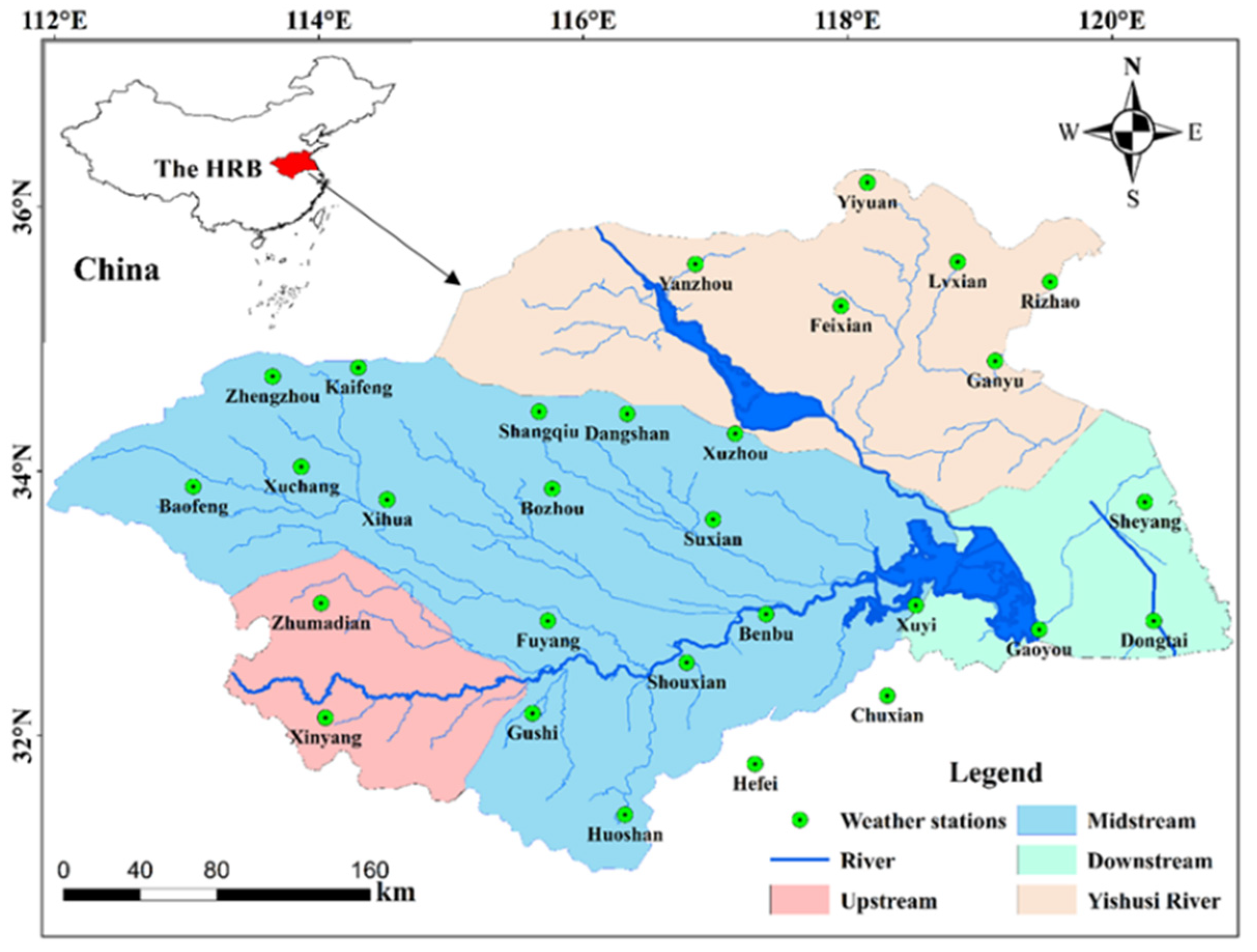
2.1. Study Area

The HRB lies between 111°55′ E~121°20′ E and 30°55′ N~36°20′ N in China, with an area of 270,000 km² (Figure 1). It is located in the East Asian monsoon zone, which is also the climate transition zone between north and south in eastern China [27,41]. The main stream of the Huai River originates in the western mountains and flows into the western Pacific Ocean from west to east. Topographically, the western, southwestern, and northeastern parts of the basin are mountainous and hilly areas, while the rest of the watershed is a vast, low–altitude plain. The annual average water surface evaporation in the river basin ranges from 900 mm to ~1500 mm, with evaporation being lower in the south and higher in the north. Specifically, the evapotranspiration in mountainous and hilly regions is relatively low, while it is higher in plain and basin areas.

Moreover, the watershed is densely populated and fertile, making it one of the most important agricultural bases in China. However, due to susceptibility to droughts and floods, as well as severe water quality degradation, the basin faces significant challenges in terms of socio–economic development and ecosystem services [42,43]. Therefore, in–depth research on the characteristics of summer ETp changes and the contributions of meteorological factors to summer ETp would provide necessary information for basin water resource utilization and agricultural production.

2.2. Data

In this study, a set of 29 national meteorological stations (

Table 1. Information about the weather stations used in this study.

No.1 a	Name	Latitude (°N)	Longitude (°E)	Elevation (m)
1	Baofeng	33.88	113.05	136.40
2	Zhengzhou	34.72	113.65	110.40
3	Xuchang	34.03	113.87	66.80
4	Zhumadian	33.00	114.02	82.70
5	Xinyang	32.13	114.05	114.50
6	Kaifeng	34.78	114.30	73.70
7	Xihua	33.78	114.52	52.60
8	Gushi	32.17	115.62	42.90
9	Shangqiu	34.45	115.67	50.10
10	Fuyang	32.87	115.73	32.70
11	Bozhou	33.87	115.77	37.70
12	Huoshan	31.40	116.32	86.40
13	Dangshan	34.43	116.33	44.20
14	Shouxian	32.55	116.78	22.70
15	Yanzhou	35.57	116.85	51.70
16	Suxian	33.63	116.98	25.90
17	Xuzhou	34.28	117.15	41.20
18	Hefei	31.78	117.30	27.00
19	Benbu	32.92	117.38	21.90
20	Feixian	35.25	117.95	121.20
21	Yiyuan	36.18	118.15	305.10
22	Chuxian	32.30	118.30	27.50
23	Xuyi	32.98	118.52	40.80
24	Lvxian	35.58	118.83	107.40
25	Ganyu	34.83	119.12	3.30
26	Gaoyou	32.80	119.45	5.40
27	Rizhao	35.43	119.53	36.90
28	Sheyang	33.77	120.25	2.00
29	Dongtai	32.87	120.32	4.30

Note: ^a Stations are arranged in ascending order of longitude.

) distributed across the basin were collected from the National Climatic Centre of China (http://data.cma.cn/, accessed on 5 March 2022) for the period 1960–2020. The dataset includes sunlight hours (Sh), mean temperature (Tm), wind speed (Ws), relative humidity (Rh), maximum temperature, minimum temperature, vapor pressure, etc., at a daily time step, which are the main meteorological factors determining ETp [1,24]. These data undergo strict quality control before being released. Only stations with complete records are selected to ensure the reliability and accuracy of the results.

3. Methodology

3.1. Penman–Monteith Method

The HRB has a humid climate, with a multi–year average precipitation of 800 mm [41]. The Penman–Monteith model is suitable to estimate the ETp in the HRB, which is shown as follows:

$$ETp={\displaystyle \frac{1}{\Delta +\gamma \left(1+0.34U_2\right)}}\left[0.408\Delta \left(R_n-G\right)+{\displaystyle \frac{900\gamma U_2}{Tm+273}}\left(e_s-e_a\right)\right]$$

(1)

where ETp is the daily potential evapotranspiration, mm/day; Δ is the slope of the saturated vapor pressure versus air temperature curve, kPa/°C; γ is the psychrometric constant, kPa/°C; U₂ is the wind speed at 2 m height, m/s; R_n is the net radiation, MJ/(m²·d); G is the heat flux density at the soil surface, MJ/(m²·d); Tm is the mean daily air temperature at 2 m height, °C; e_s is the saturation vapor pressure, kPa; e_a is the actual vapor pressure (kPa); and (e_s − e_a) is the saturation vapor pressure deficit, kPa.

3.2. Sensitivity Analysis

The perturbation method [1,44] is a popular and practical method of sensitivity analysis, which is on the basis of the presupposed linear perturbation–response relationship between ETp and meteorological factors. It involves two sequential steps: first, adjusting a single meteorological variable by a small percentage change relative to its baseline value, while holding other variables constant; and second, calculating the corresponding magnitude of ETp variation induced by each perturbation. In this study, it was also used to evaluate the sensitivity of summer ETp to different meteorological variables in the HRB.

The formula of the perturbation method is as follows:

$$S_{k,i}={\displaystyle \frac{ET{p}_{k,i}(r)-ET{p}_{k,i}(-r)}{2r\cdot ET{p}_i(t)}}$$

(2)

where S_k,i is the relative sensitivity coefficient of ETp to the kth factor at the ith year; r is the perturbation ratio of meteorological factors, expressed as a small percentage change in meteorological factors relative to the current level, with r = 1% in the study; ETp_k,i is the disturbed ETp in response to the kth meteorological factor and its daily value in the ith year is disturbed under the perturbation ratio r; and t is the time scale (1–day ≤ t ≤ 1–year). In this study, all time scales were calculated on a 1–day scale basis, and four climatic factors (i.e., Sh, Tm, Ws, and Rh) are considered for sensitivity analysis.

If S_k,i > 0, it illustrates that ETp increases with the increase in the climate factor, and if S_i < 0, it means that ETp will decrease with the increase in the climate parameters. The larger the |S_k,i|, the greater the impact of meteorological factors on summer ETp. In this study, four climatic factors (i.e., Sh, Tm, Ws, and Rh) are considered for sensitivity analysis.

3.3. Anomaly Contribution Analysis Method

The anomaly contribution analysis method [1] was used to quantitatively calculate the annual contribution rate of summer climate factors to summer ETp by considering the physical and statistical relationship between meteorological element anomaly rate and ETp anomaly rate.

The steps of this method are as follows:

• Step 1: Calculate the relative variations in meteorological factors x_k and ETp against their multi–year average values:

  $$\left\{\begin{array}{l}{\theta }_{k,i}(t)={\displaystyle \frac{x_{k,i}(t)-\overline{x_k}}{x_{k,i}\left(t\right)}}\\ {\varphi }_i\left(t\right)={\displaystyle \frac{ET{p}_i\left(t\right)-\overline{ETp}}{ET{p}_i\left(t\right)}}\end{array}\right.$$

  (3)

  where θ_k,i(t) is the anomaly ratio of meteorological element k in year i during the study period; $\overline{x_k}$ is the average of meteorological element k; ϕ_i(t) is the anomaly ratio of ETp in year i during the studying period; and $\overline{E{T}_p}$ is the average of ETp (t) during the studying period.
• Step 2: Calculate the contribution of each climate factor x_k to the ETp:

  $${\gamma }_{k,i}=S_{k,i}\cdot {\theta }_{k,i}$$

  (4)

  where γ_k,i is the contribution of x_k to ETp at the ith year, and S_k,i is the sensitivity coefficient of ETp to the kth factor at the ith year.
• Step 3: Calculate the total contribution of all the climatic factors to the ETp:

  $${\psi }_i={\displaystyle \sum _{k=1}^m{\gamma }_{k,i}}$$

  (5)

  where ψ_i is the total contribution of all the climatic factors to the ETp at the ith year, and m is the number of meteorological elements considered.
• Step 4: Determine the relationship between ϕ_i and ψ_i with the Pearson correlation coefficient and the Sen’s trend slope:

  $$R={\displaystyle \frac{{\displaystyle {\sum }_i^n\left({\varphi }_i-\overline{\varphi }\right)\left({\psi }_i-\overline{\psi }\right)}}{\sqrt{{\displaystyle {\sum }_{i=1}^n{\left({\varphi }_i-\overline{\varphi }\right)}^2}}\sqrt{{\displaystyle {\sum }_{i=1}^n{\left({\psi }_i-\overline{\psi }\right)}^2}}}}$$

  (6)

  where $\overline{\varphi }$ and $\overline{\psi }$ are the averages of ϕ_i and ψ_i, respectively.

The Sen’s trend slope [1] of (ϕ_i, ψ_i) data series is estimated by:

$$\beta =Median\left({\displaystyle \frac{{\psi }_j-{\psi }_i}{{\varphi }_j-{\varphi }_i}}\right),\forall j>i.$$

(7)

where Median () is the function that calculates the median of a given sequence.

The value of 1–R shows the degree to which the relationship between ϕ_i and ψ_i is linearly positive, and the value of |1 − β| indicates the degree to which a linear positive relationship satisfies the function y = x. The smaller the deviation between R and β and 1.0, the smaller the difference between ϕ_i and ψ_i. In this study, ΔR = 0.1, and Δβ = 0.2 are set as the tolerance limits [1] for R and β, respectively. Then, the next step can be taken.

• Step 5: Calculate the relative contribution rate of a meteorological factor to the ETp:

  $$C_{k,i}={\displaystyle \frac{{\gamma }_{k,i}}{{\displaystyle \sum _{k=1}^m\left|{\gamma }_{k,i}\right|}}}$$

  (8)

  where C_k,i is the relative contribution rate of the kth meteorological factor to the ETp at the ith year, %. A positive (or negative) contribution rate indicates that the change of local climate factors improves (or reduces) ETp, while the absolute value of the contribution rate indicates the impact of the climate factors variations on ETp change. For the ETp, a climatic factor with the maximum |C_k,i| is called the dominant meteorological factor. More details can be found in Liu et al. (2023) [1].

Based on the summer contribution rate of each climatic element, the dynamic changes in the contribution of climate factors to summer Etp can be revealed, which helps to demonstrate the specific impact of climate elements on ETp in this region.

3.4. Trend Test and Change Point Identifying

The Mann–Kendall trend test (MK) is employed to assess the trend in the ETp and climatic factors time series in this study. Since the results of the MK test are easily influenced by autocorrelation [45], the trend–free prewhitening (TFPW) approach was applied to eliminate serial correlation in the ETp and climatic time series. More details can be found in Liu et al. (2022) [46]. A significance level of 95% was used to evaluate whether the detected trend was statistically significant or not in the study.

Moreover, the abrupt change points were identified with the usage of the heuristic segmentation method. It is a commonly used method to detect change points in non–linear and non–stationary time series based on sliding T test [47]. The principle of this method is to divide a time series into two subsequences with a moving segmentation point, and compare the significance of their averages’ difference at the 95% confidence level with a threshold of P₀(=0.95), then obtain the change point. When the obtained significance value is less than the P₀ or the obtained subsequence length is shorter than the minimum length l (l = 25), the change point recognition process ends. More details about the method can be found in Liu et al. (2019) [47]. The research framework of this study is shown in Figure 2.

4. Results

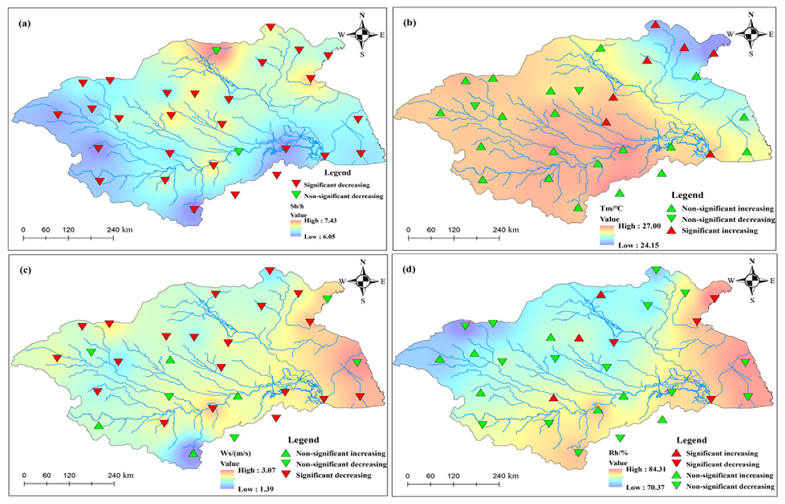
4.1. Trends of Summer Meteorological Factors

Figure 3 shows the spatial distribution of multi–year mean values of summer Sh, Tm, Ws, and Rh across the basin and their trends detected by TFFPW–MK. There are significant differences in the range and trends of mean summer meteorological parameters. Figure 3a shows that the average summer sunshine duration varies from 6.05 h to 7.43 h during 1960–2020, with longer sunlight appearing in the northeast of the basin. Moreover, there is a significant decreasing trend of Sh at a confidence of 95% across the basin. Figure 3b indicates that there are apparent increasing trends of summer Tm across the basin from 1960 to 2020, which are consistent with the global warming trend. In terms of spatial patterns, Tm (varying from 34.15 °C to 27.00 °C) has a clear southwest–northeast gradient, with higher values mostly appearing in the southwest of the basin and lower values mostly occurring in the northeast of the basin. Figure 3c demonstrates that long–term averages of Ws range from 1.39 m/s to 3.07 m/s. In addition, significant decreasing trends of Ws are clearly dominant, with only four stations exhibiting a non–significant upward trend. For Rh shown in Figure 3d, a higher Rh usually occurs in the northeast of the basin, with variation between 70.37% and 84.31%. Moreover, Rh mainly shows mixed trends since the number of stations with increasing and decreasing trends is basically the same.

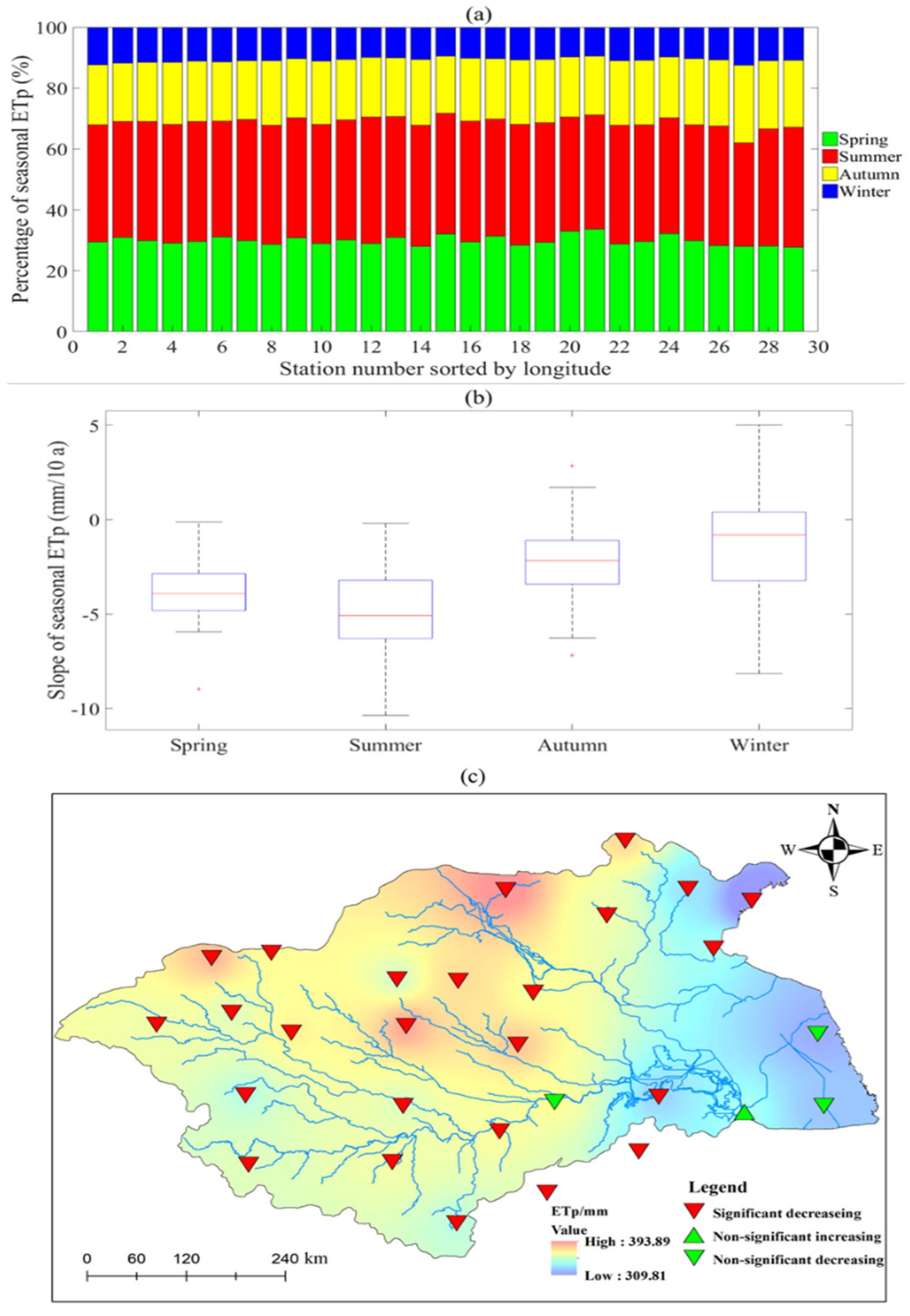
4.2. Changing Characteristics of Summer ETp

Figure 4 demonstrates the multi–year average percentages and trend slopes of ETp in four seasons of the HRB. It can be seen from Figure 4a that the annual ETps at the 29 stations are concentrated in summer, and the percentage of summer ETp ranges from 34% to 42%. Figure 4b shows that the ETp tends to decrease in all four seasons. Specifically, the summer ETp has the fastest downward trend with a trend slope of −5.1 mm/10a. Hence, variation in annual ETp in the basin is mainly dominated by summer ETp, which further illustrates the necessity of studying ETp in summer and further illustrates the necessity of studying ETp in summer. Figure 4c shows that summer ETp varies from 309.12 mm to 393.83 mm, exhibiting an obvious southwest–northeast gradient, with higher values mostly occurring in the southwest of the basin and lower values mostly appearing in the northeast of the basin. In addition, there are 26 stations showing significant downward trends in summer ETp.

Figure 5a shows an example of identifying the change points in the summer ETp time series of Dangshan station. The blue line in Figure 5a represents the first change point detection process. The maximum T of the first iteration was discovered in 2001, corresponding to P (T_max) = 1.0 > P₀ = 0.95, indicating that 2001 is a change point in the summer ETp time series. As the length of the subsequence 1960–2001 is greater than 25, the recognition process continues. Similarly, the second change point appeared in 1970, represented by an orange line. Then, the third iteration and segmentation process began of the subseries 1971–2001, illustrated by the green line with the third maximum value T that appeared in 1980. However, it is not another change point, as the corresponding P (Tmax) = 0.86 < P₀ = 0.95. Finally, the recognition process ends.

Due to the detection of two change points in 1970 and 2001, the original summer ETp series of Dangshan station can be divided into three sub–series. To better illustrate the reliability of the identified change points, Figure 5b shows a comparison of the average values of these sub–series segmented by the change points. The results show significant differences in the average values of the three periods: 409.2 mm from 1960 to 1970, 370.8 mm from 1971 to 2001, and 324.6 mm from 2002 to 2020. The red arrows in Figure 5b demonstrate the direction of change in averages of summer ETp, indicating a sharp decline in different times of summer ETp at Dangshan station between 1960 and 2020.

Table 2. Change points of summer ETp and meteorological factors.

No.1	Stations	ETp	Sh	Tm	Ws	Rh
1	Baofeng	1979	1980	——	1977, 2006	1970
2	Zhengzhou	1975	1975, 1995	1970, 2008	1977	1970, 2008
3	Xuchang	1970	1970, 2002	1970	1982, 2006	1970
4	Zhumadian	1975	1980	——	2002	——
5	Xinyang	1979	1980, 2002	——	1980, 2005	——
6	Kaifeng	1970	1997	1970, 2008	1973	1970, 2004
7	Xihua	1979	1975, 2002	——	1986	——
8	Gushi	1980	1980, 2002	——	1983, 2005	——
9	Shangqiu	1979	1980	——	1979, 1990	——
10	Fuyang	1980	1980, 2002	——	1971	——
11	Bozhou	1971	1980	——	1979, 2001	1970, 2009
12	Huoshan	1972	1979	——	1973, 1989	——
13	Dangshan	1970, 2001	1980	——	2001	2002
14	Shouxian	1980	1980	——	2005	——
15	Yanzhou	1970	1979	——	2003	——
16	Suxian	1979	1980, 2002	1993	1979	2008
17	Xuzhou	1979	1979	2009	1986	2009
18	Hefei	1970	1970, 1992	——	1972, 2006	——
19	Benbu	——	1980	——	1978, 2001	——
20	Feixian	1984	1993	2009	1979, 2003	——
21	Yiyuan	1984	1988	——	1979	——
22	Chuxian	1972	1979	——	1978, 2002	——
23	Xuyi	1979	1979, 1990	——	1970, 1990, 2003	2009
24	Lvxian	1970	1970, 1983, 1993	——	1979	——
25	Ganyu	1997	1981, 1997	——	1992, 2003	1991
26	Gaoyou	——	1979	2000	1985	1991, 2001
27	Rizhao	2005	2002	1993	1991, 2002	1992
28	Sheyang	——	1970	——	——	——
29	Dongtai	——	1979	2003	——	1993

summarizes the change points in the summer ETp time series. Generally speaking, change points of summer ETp are mainly concentrated around the 1970s and 1980s.

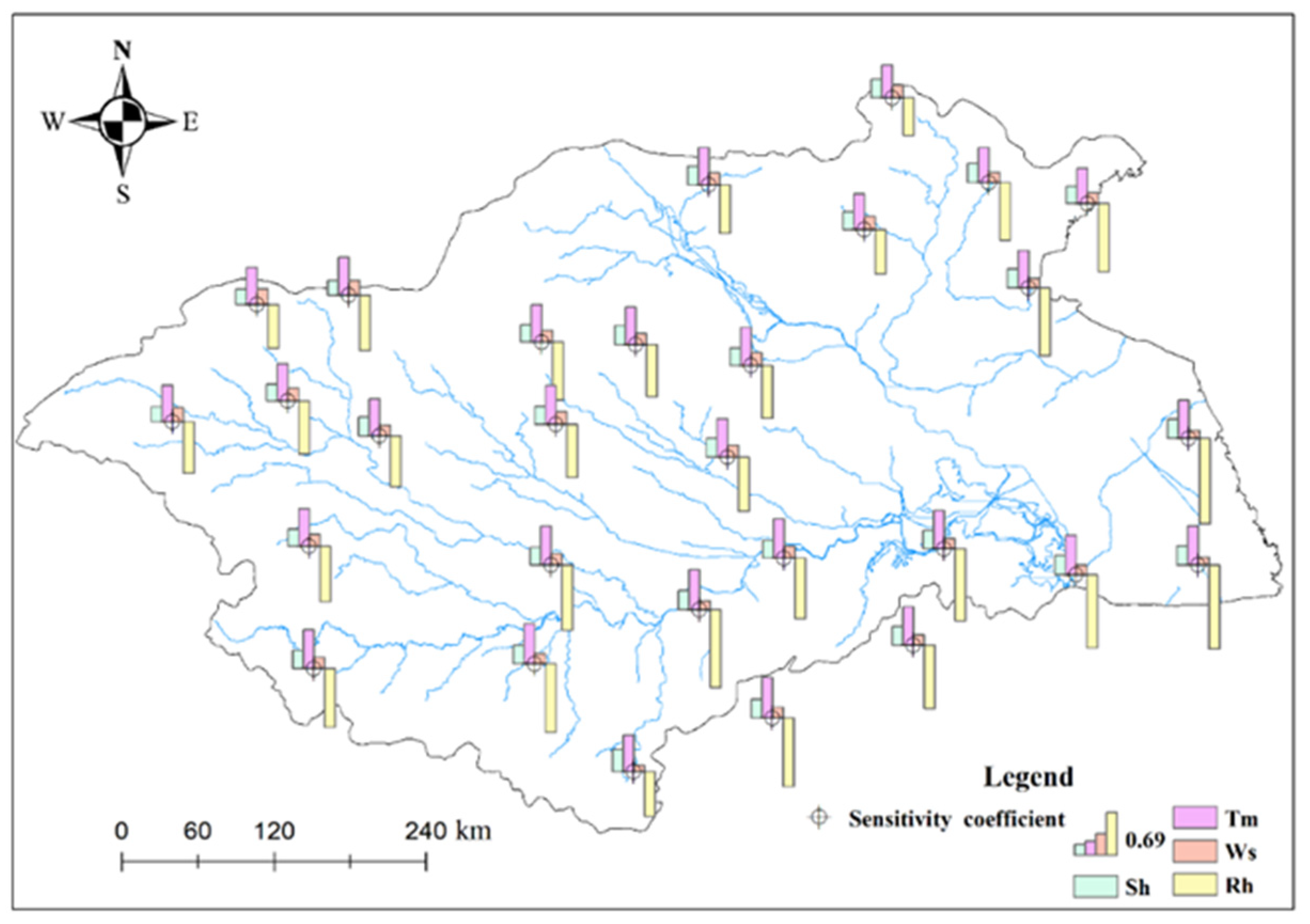
4.3. Sensitivity of ETp to Meteorological Factors in Summer

Figure 6 shows the spatial distribution of sensitivity coefficients of summer ETp to Sh, Tm, Ws, and Rh. The sensitivity coefficient histogram of each site not only reflects their size but also reveals their positive and negative impacts on summer ETp. It can be observed that different meteorological parameters usually have different influences on ETp. The sensitivity coefficients of Sh, Tm, and Ws are all positive, indicating that they have positive impacts on summer ETp. In particular, summer ETp will increase with the increases of Sh, Tm, and Ws. In contrast, the sensitivity coefficients of Rh are negative, indicating a negative impact on summer ETp, meaning summer ETp will decrease with the increase in Rh. In addition, the variation range of the sensitivity coefficient is also different. For Sh, Tm, and Ws, their sensitivity coefficients vary between 0.24 and 0.36, 0.53 and 0.65, and 0.10 and 0.25, respectively. The sensitivity coefficient of Rh is highest at −0.61 and lowest at −1.39. According to the absolute values of the sensitivity coefficients of Sh, Tm, Ws, and Rh, it is found that the sensitivity of summer ETp in the basin to meteorological factors can be ranked in descending order as Rh > Tm > Sh > Ws.

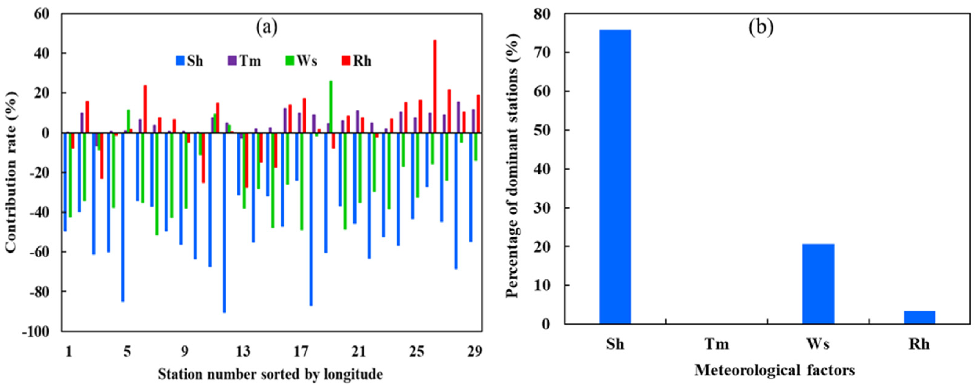
4.4. Contribution Patterns of Summer Meteorological Factors to Summer ETp

4.4.1. Contribution Analysis at Multi–Year Scale

Before using the anomaly contribution analysis method to get the annual contribution rate of summer climate factors to summer ETp, we first calculated the multi–year contributions of summer Sh, Tm, Ws, and Rh to summer ETp in the HRB, and the results are shown in Figure 7. As shown in Figure 7a, although summer ETp is most sensitive to Rh, Sh and Ws contribute the most to the changes in summer ET, and Tm has the smallest contribution rate. Specifically, the relative contribution rates of summer Sh, Ws, Rh, and Tm vary from −90.4%~−23.8%, −51.5%~26.0%, −27.5%~46.5%, and −6.7%~15.3%, respectively. Figure 7b displays the percentages of stations where summer ETp is dominated by the four summer meteorological factors (Sh, Tm, Ws, and Rh) at a multi–year scale. It shows that summer Sh, Ws, and Rh are the dominant contributing factors of summer ETp in the HRB since the percentages of stations dominated by summer Sh, Ws, and Rh are 75.9%, 20.7%, and 3.4%, respectively. Meanwhile, summer Tm is never a dominant factor, although it has some influence on summer ETp in the basin (see Section 4.3).

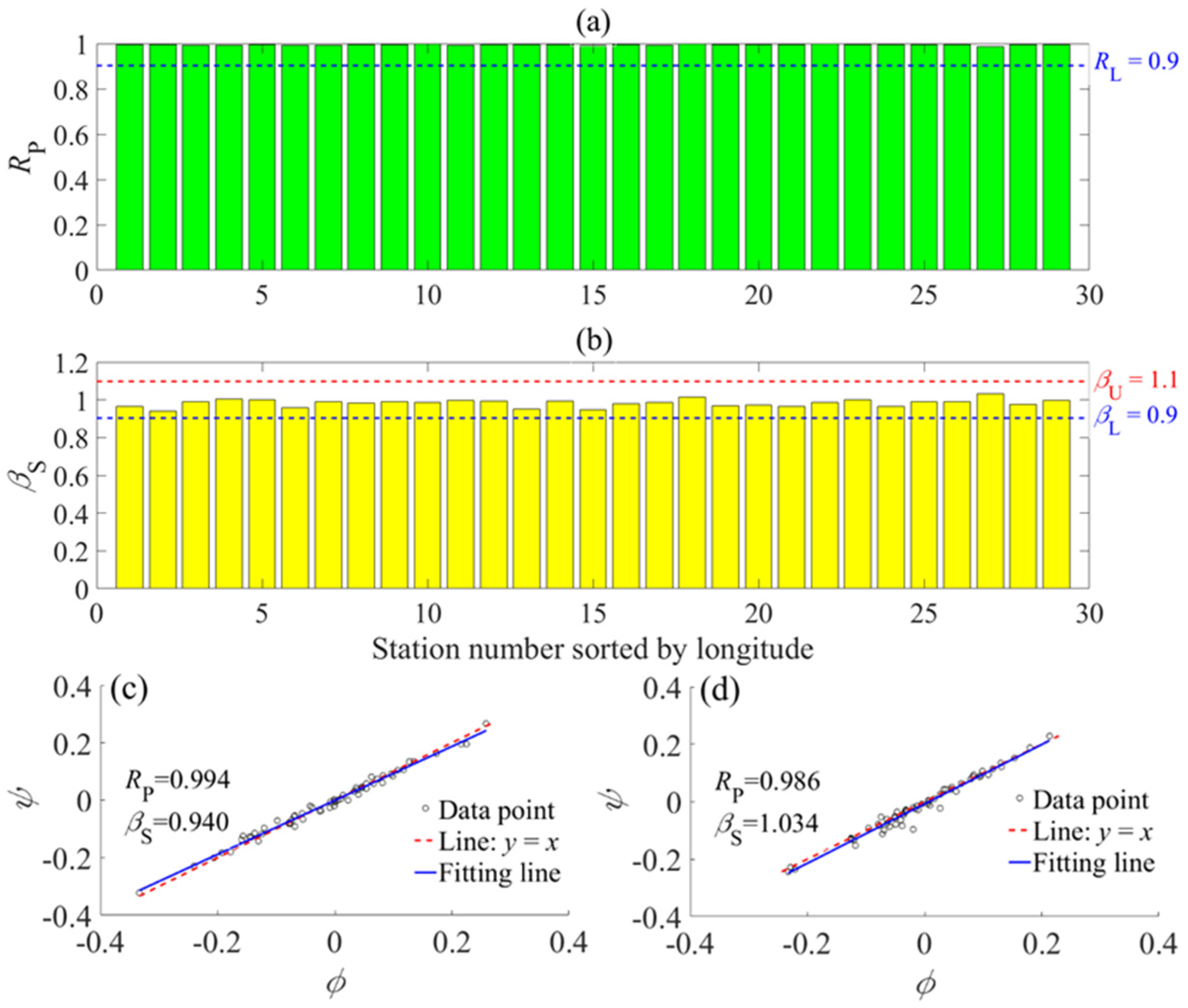
4.4.2. Application of Anomaly Contribution Analysis

Figure 8 illustrates the results of the applicability test results of the anomaly contribution analysis in the HRB in the summer. It shows that the Pearson correlation coefficient (R_P) between the relative variation in summer ETp (ϕ) and the total contribution of summer meteorological factors (ψ) ranges from 0.986 and 0.998, which are larger than the allowable lower bound R_L (Figure 8a). In addition, the Sen’s trend slopes (β_S) of (ϕ, ψ) data points vary between 0.940 and 1.034 for the 29 stations (Figure 8b), which are within the allowable range of (β_L, β_U).

It is worth noting that among the 29 stations, the Zhengzhou and Rizhao stations performed the worst in the anomaly contribution analysis. Figure 8c,d show that the β_S of Zhengzhou station is 0.940, with a maximum deviation of 1.0, and the R_P of Rizhao station is 0.986 with a maximum difference of 1.0. However, the (ϕ, ψ) data points of the two stations are still distributed around the line y = x, implying that ψ fits ϕ well. Therefore, the anomaly contribution analysis method is able to accurately assess the annual contributions of the four meteorological factors (Sh, Tm, Ws, and Rh) to ETp in summer.

4.4.3. Contribution Analysis Based on the Anomaly Contribution Analysis

(1)

Spatiotemporal distributions of contributions

The relative contribution rates of Sh, Tm, Ws, and Rh to ETp in the HRB in summer are shown in Figure 9. Variations in the relative contribution rates of the four meteorological factors with longitude and latitude are displayed in Figure 9a–d and Figure 9e–h, respectively. In addition, the contribution of a factor to summer ETp is considered significant when the absolute value of the relative contribution rate is greater than 30% in this study.

For Figure 9a,e, the relative contribution rate of summer Sh varies from −91.4% to 92.0%. Specifically, the relative contribution rate of summer Sh is mainly positive in the period 1961–1980, and more than 75% of station–years have a significant contribution. During the period 1981–1999, the relative contribution of summer Sh shows great fluctuations, with significant negative contributions in 37% of station–years and significant positive contributions in 27% of station–years. For the period 2000–2013, more than 73% of station–years have a significant negative contribution. After 2013, summer Sh has a significant negative contribution during 2015–2017.

Figure 9b,f show that the relative contribution rate of summer Tm to summer ETp ranges from −78.4% to 81.1%, and it is insignificant for 88% of station–years. The positive contribution of summer Tm is significant in 1962, 1995, 2014, and 2017–2020, while the negative contribution is significant in 1977, 1983–1984, and 1987–1988.

In Figure 9c,g, the relative contribution rate of summer Ws to summer ETp varies from −89.8% to 87.4%. Overall, 9% of station–years have a significant negative contribution, while 7.5% of station–years have a significant positive contribution. The stations with significant positive contributions are mainly in the northern part of the basin in 1961–1964 and 1974–1977, and in the central part of the basin in 1995–2000 in the east–west direction. Moreover, the stations with a significant negative contribution were basically distributed in the central and northern regions of the basin in 2010–2018.

Figure 9d,h illustrate that the relative contribution rate of summer Rh is between −86.6% and 80.5%. It can be observed that 20% of station–years have a significant negative contribution, and 14% of station–years have a significant positive contribution. Specifically, summer Rh has a significant negative contribution in the eastern region during 1961–1964 and 1971–1977, in the northern region during 1990–1992 and 1999, in the northwestern region during 1996–1997, and across the basin during 1985–1986. Moreover, summer Rh has a significant positive contribution in the southwestern area during 2005–2007, and in the whole basin during 1965–1970, 1993, 1998, 2002–2003, and 2010–2014.

(2)

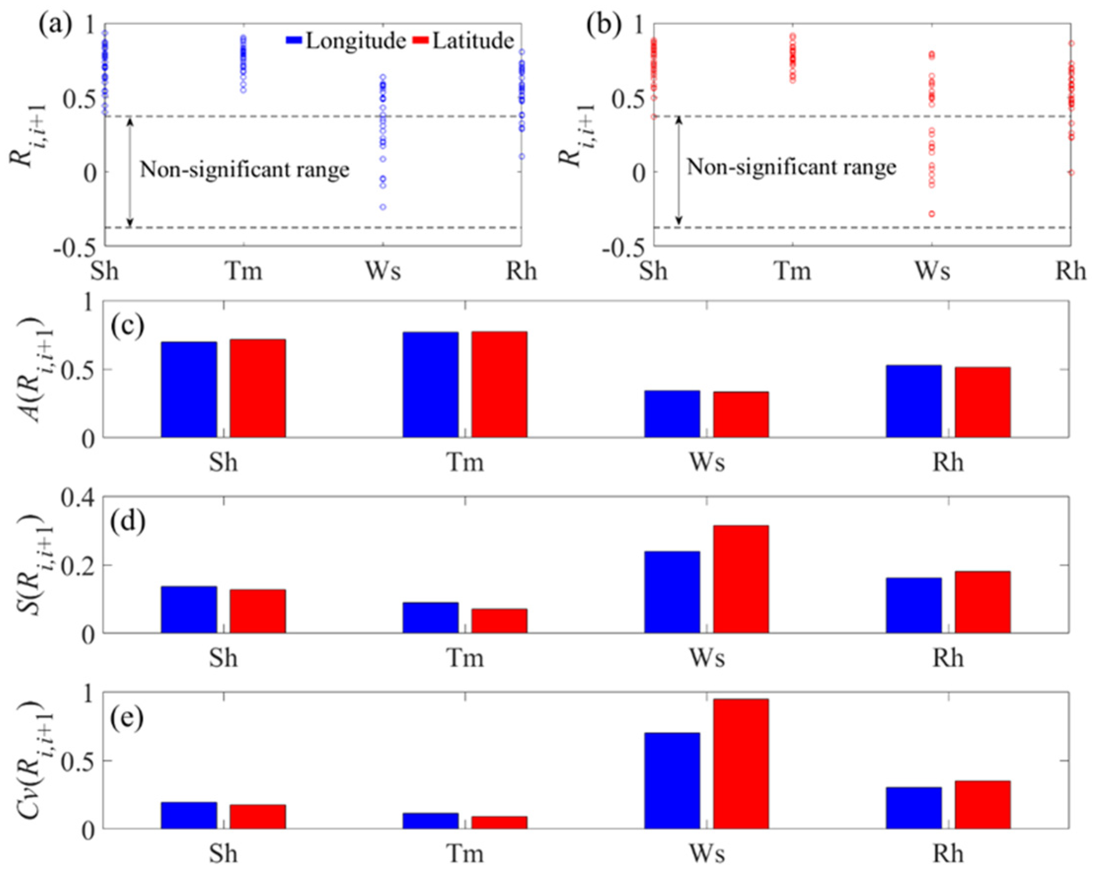
Spatial correlations of contributions

Figure 10a,b demonstrate the contribution correlation coefficients of meteorological factors for neighboring stations in longitude and latitude, respectively. Note that there are 28 pairs of adjacent stations in the HRB in longitude or latitude. It can be observed in Figure 10a that the contribution correlation coefficients of summer Sh are consistently significant for the 28 pairs of stations in longitude, as well as for summer Tm. For summer Ws, the contribution correlation coefficients are significant only for 14 pairs of stations in longitude. As to summer Rh, the contribution correlation coefficients are significant for 24 pairs of stations in longitude. Figure 10b shows that the contribution correlation coefficients of summer Sh, Tm, Ws, and Rh are significant for 27, 28, 15, and 23 pairs of stations in latitude, respectively.

In Figure 10c, the average contribution correlation coefficients of summer Sh (Tm, Ws, and Rh) are 0.697 (0.765, 0.341, and 0.528) and 0.716 (0.770, 0.333, and 0.514) for the 28 pairs of stations in longitude and latitude, respectively. Figure 10d shows that the standard deviations of the contribution correlation coefficient of summer Sh (Tm, Ws, and Rh) are 0.137 (0.090, 0.239, and 0.162) and 0.127 (0.078, 0.314, and 0.180) for the 28 pairs of stations in longitude and latitude, respectively. Furthermore, Figure 10e exhibits the variation coefficients of the contribution correlation coefficient of summer Sh (Tm, Ws, and Rh) for the 28 pairs of stations in longitude and latitude. The variation coefficient for summer Sh (Tm) in longitude is slightly more than that for summer Sh (Tm) in latitude, while the variation coefficient for summer Ws (Rh) in longitude is obviously less than that for summer Ws (Rh) in latitude.

(3)

Dominant meteorological factors

Figure 11 shows the percentages of years in which summer ETp is dominated by summer Sh, Tm, Ws, and Rh in the HRB. From Figure 11a, it can be seen that the percentages of years dominated by different meteorological factors vary from station to station. Specifically, the percentages of years dominated by summer Sh, Tm, Ws, and Rh are 39.2%~81.7%, 1.7%~15%, 0~30%, and 10%~40%, respectively. On average across the 29 stations, the percentages of years dominated by summer Sh, Tm, Ws, and Rh are 61.3%, 6.8%, 9.5%, and 22.4%, respectively. This implies that summer Sh and Rh are the two most important dominant factors for summer ETp, while summer Tm is the least important influencing factor. In addition, Figure 11b demonstrates that the percentage of years dominated by summer Tm has a significant increasing trend with longitude. Figure 11c shows that the percentage of years dominated by summer Sh has a significant downward trend with latitude. As regards summer Ws and Rh, the percentages of years dominated by them are not clearly related to longitude or latitude.

5. Discussion

5.1. Anachronistic Evaporation Paradox for Summer ETp

Previous research has reported increases and decreases in annual ETp in different regions over the past few decades. However, our research further indicates that the summer ETp also varies. Summer is generally the most vigorous season of the year for ETp due to abundant solar radiation and high temperature [36], which has also been confirmed in the HRB (Figure 4a). Moreover, the decreasing trend in summer ETp is more obvious than that in other seasons (Figure 4b), indicating that climate change has the greatest impact on summer ETp in the basin.

The evaporation paradox has attracted widespread attention with increasing temperatures around the world. Li et al. (2023) further classified paradoxical phenomena into two types: temperature increases but ETp decreases (Type I), and temperature decreases but ETp tends to increase (Type II) [48]. They claim that in the future, these two evaporation paradoxes will coexist in China. However, for the HRB, it shows that there is an insignificant trend of summer Tm in most stations (Figure 3b), while summer ETp exhibits a significant decreasing trend at the vast majority of stations (Figure 4c). This suggests that there may be a clear trend in regional ETp even if local Tm has no significant change. In other words, the concept of the evaporation paradox might not be appropriate from the seasonal perspective.

5.2. Simple Attribution Analysis for Summer ETp Changes

From west to east, the summer climate in the HRB is increasingly influenced by the maritime climate (Figure 1). Thus, summer Tm and Rh show significant decreasing and increasing trends from west to east, respectively (Figure 3b,d). In addition, the HRB in the East Asian monsoon zone is strongly affected by the East Asian summer monsoon [49], so the summer Ws increases significantly from west to east (Figure 3c). The downward trend in summer ETp from west to east (Figure 4c) implies that in the east–west direction, the spatial trend of Tm has more influence than the spatial trends of Ws and Rh on the spatial trend of ETp in summer.

The climate varies greatly between the north and the south in the north–south climatic transition zone of eastern China, where the northern region has cooler temperatures, less humidity, fewer clouds, and less precipitation than the southern region in summer [50]. Therefore, summer Tm and Rh have significant downward trends, while summer Sh significantly increases from south to north in the basin (Figure 3a,b,d). Moreover, the insignificant trend in summer ETp (Figure 4c) from south to north indicates that the influence of the increasing trend in summer Sh offsets that of decreasing trends in summer Tm and Rh on the spatial trend of summer ETp in the north–south direction.

Trends in summer Tm and Rh have a weak influence on the trend of summer ETp in the HRB, and the decline in summer ETp should be attributed to the decrease in summer Sh and Ws during 1961–2020. Further, the fading downward trend of summer ETp is caused by the weakening decline trend in summer Sh and the enhancing upward trend in summer Tm from west to east. Additionally, the results of change points in the climatic factors (see Table 1) imply that the abrupt changes in summer Sh and Ws around the 1970s and 1980s led to the corresponding mutation in summer ETp in the watershed.

By comparing trends and abrupt changes, it can be inferred that the temporal variations in summer ETp are mainly triggered by the changes in summer Sh and Ws in the HRB. This finding is consistent with the conclusions of many previous studies on other regions or watersheds [26,32,40,51,52]. Nevertheless, simple attribution analysis based on comparisons of trends and abrupt changes could not clearly explain the specific influence of meteorological factors on ETp in summer. Taking Dangshan station as an example, the change points of ETp and meteorological factors in summer are not completely consistent. Not surprisingly, the rapid decrease in summer Ws (Figure 3c and Table 2) and the sudden increase in summer Rh (Figure 3d and Table 2) led to a sharp decrease in summer ETp (Figure 5b) after 2001. However, the sudden decrease in summer ETp in 1970 (Figure 5b) cannot be attributed to the rapid decrease in summer Sh in 1980 (Figure 3a and Table 2). Moreover, Figure 5a shows that around 1980 there was a third possible change point in summer ETp, but it was discarded due to failure to pass the abrupt change test. Therefore, simple attribution analysis can provide important clues, but not sufficient evidence, for the influence of meteorological factors on ETp in summer.

5.3. Anomaly Contribution Analysis for Summer ETp Changes

The anomaly contribution analysis can feasibly estimate the contributions of different meteorological factors to ETp in the HRB in summer (Figure 8). It can demonstrate the spatiotemporal contribution patterns of summer meteorological factors to summer ETp (Figure 9). Throughout the study period, the contributions of summer Sh, Tm, Ws, and Rh are characterized by step–shifts and/or positive–negative alterations. Specifically, the contributions of summer Sh and Ws show strong and weak step–shifts from positive to negative, respectively. The contributions of summer Rh and Tm have strong and weak positive–negative alterations, respectively. Moreover, the contribution of summer Sh displays synchronous changes across the HRB, as do summer Tm and Rh. In comparison, there is a clear concentration of spatial variation in the contribution of summer Ws.

The contribution correlation coefficients of summer Sh, Tm, and Rh are significant for most pairs of neighboring stations, while the contribution correlation coefficients of summer Ws are insignificant for most pairs of stations (Figure 10a,b). In addition, the contribution correlation coefficients of summer Sh and Tm have lower variation coefficients in latitude than in longitude, while those of summer Ws and Rh have lower variation coefficients in longitude than in latitude (Figure 10e). Therefore, the contributions of summer Sh and Tm have the best spatial homogeneity, followed by summer Rh. The contribution of summer Ws exhibits an obvious distribution pattern of spatial heterogeneity. Moreover, the contributions of summer Sh and Tm have better spatial homogeneity in latitude than in longitude, and the contributions of summer Ws and Rh have better spatial homogeneity in longitude than in latitude.

In analyzing the trends of meteorological factors, it is found that summer Sh in the entire HRB shows a significant decreasing trend. However, this decreasing trend is gradually weakening from south to north (Figure 3a), which is why the percentage of years dominated by summer Sh also decreased from south to north (Figure 11c). Similarly, the percentage of years dominated by summer Tm is increased from west to east (Figure 11b), which can be attributed to the increasing rate of warming along this spatial direction in the HRB (Figure 3b). Therefore, the influence of summer Tm on summer ETp is enhanced from west to east, while that of summer Sh is weakened from south to north in the watershed.

5.4. Differences in Dominant Meteorological Factors at Different Scales

There are significant differences in the sensitivity of ETp to different meteorological factors in different geographical locations and climatic conditions. Du et al. (2022) found that ETp of Loess Plateau was most sensitive to Rh at the annual scale, Tm in summer, and Rh in winter [34]. Hamed et al. (2023) held that ETp was most sensitive to Ws in the Middle East and North Africa over the study period [3]. In this study, sensitivity analysis results (Figure 6) indicate that the sensitivities of summer ETp to meteorological elements in the HRB are, in descending order, Rh, Tm, Sh, and Ws. Sensitivity analyses do help to assess the response of ETp to different meteorological factors in a specific geographic setting [44,53]. However, the sensitivity analyses did not consider the effect of the variation magnitude in meteorological factors on ETp, making it difficult to identify the dominant meteorological factors for ETp.

The multi–year contribution analysis shows that summer Rh is a dominant factor in summer ETp, whereas summer Tm is not in the HRB (Figure 7). A clue to this finding cannot be obtained from the simple attribution analysis and the sensitivity analysis results mentioned above. Moreover, the multi–year contribution analyses show that summer Sh and Ws are the two most important factors contributing to the trend in summer ETp in the HRB, which is supported by Li et al. (2018) [24]. Multi–year contribution analyses are able to quantify the contribution of meteorological factor trends to ETp trends [34,35], but fail to show the temporal changes in dominant meteorological factors for ETp.

In contrast to the simple attribution analysis, sensitivity analysis, and multi–year contribution analysis, the anomaly contribution analysis could accurately reveal detailed driving patterns of different meteorological factors and identify the dominant meteorological factors for summer ETp. Specifically, the anomaly contribution analysis results indicate that the variations in summer ETp are mainly controlled by summer Sh, followed by summer Rh in the HRB. Summer Sh has significant contributions to summer ETp at most station–years, and summer Rh has more station–years with significant contributions than summer Tm and Ws (Figure 9). This finding is supported by the results in Figure 11a, where the percentage of years controlled by summer Sh is the highest on average, followed by summer Rh.

As regards the second dominant meteorological factor of summer ETp, the anomaly and multi–year contribution analyses diverged, with the anomaly contribution analysis suggesting summer Rh and the multi–year contribution analysis supporting summer Ws. The reason lies that the contribution of summer Rh has a stronger positive–negative alteration, which offsets the overall contribution of summer Rh to the trend in summer ETp during the study period.

The dominant factors of ETp may be different at the multi–year and seasonal scales in the same region, which is consistent with Liu et al. (2023) [1]. Moreover, Liu et al. (2023) found that Ws is not the dominant meteorological factor of ETp of the entire HRB in summer, while this study confirms that summer Ws is a dominant factor of summer ETp at most stations in the basin though its contribution is small on average [1]. This finding implies that the contributions of summer meteorological factors to summer ETp have a non–ignorable scale effect [54] for the HRB.

6. Conclusions

Taking the Huai River Basin as an example, this study investigated the dynamic changes in summer ETp during 1960–2020, then assessed the contributions of four meteorological factors (Sh, Tm, Ws, and Rh) to summer ETp variations, and finally analyzed the spatiotemporal patterns of the four contribution factors using the newly developed anomaly contribution analysis method. The main conclusions are as follows:

(1)

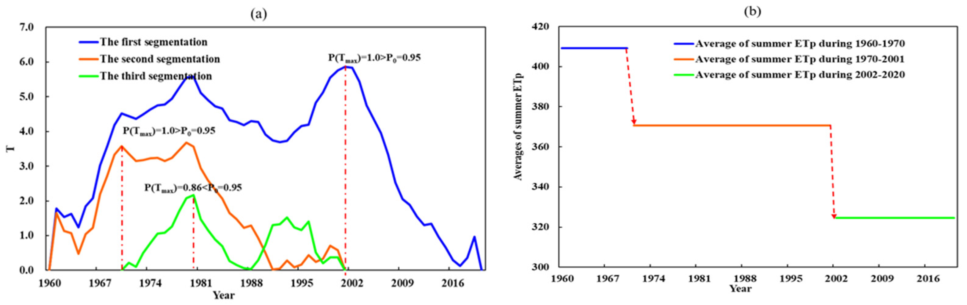
There is a significant decreasing trend in the summer ETp but the trend in summer Tm is insignificant at most stations of the basin, suggesting the evaporation paradox might not be appropriate from the seasonal perspective. In addition, summer ETp experienced an abrupt change around the 1970s and 1980s because of the mutations in summer Sh and Ws, indicating the nonstationarity of the summer ETp series.

(2)

Sensitivity analysis demonstrates the sensitivity of summer ETp in the basin to meteorological factors can be ranked in descending order as Rh > Tm > Sh > Ws. However, the two most important dominant meteorological factors of summer ETp are summer Sh and Ws at the multi–year scale, while they are summer Sh and Rh at the seasonal scale, suggesting the dominant factors of ETp may be different at the multi–year and seasonal scales in the same region. Moreover, the dominant meteorological factors of summer ETp are also different at station and basin scales due to scale effects.

(3)

Dynamic changes in contribution rates show that summer Sh and Ws have significant step–shifts from positive to negative throughout the study period, while the contributions of summer Rh and Tm show clear positive–negative alterations. Except for summer Ws, the contributions of summer Sh, Tm, and Rh show good spatial homogeneity. Moreover, the contributions of summer Sh and Tm have better spatial homogeneity in the north–south direction, while the contributions of summer Ws and Rh have better spatial homogeneity in the east–west direction.

This study primarily focuses on local meteorological factors that dominate the changes in ETp during summer in the HRB, without delving into the impact of large–scale climatic factors on ETp changes. Therefore, it is necessary to conduct in–depth research on the effect of large–scale oceanic–atmospheric patterns on regional ETp changes in the future. Moreover, the research framework of this article, especially the anomaly contribution analysis method, is also applicable to other regions and not limited to East Asia.

References

1. Liu, S.; Xie, Y.; Fang, H.; Xu, P.; Du, H. A method for identifying the dominant meteorological factors of atmospheric evaporative demand in mid-long term. Water Resour. Res. 2023, 59, e2022WR033321. [Google Scholar] [CrossRef]
2. Gharbia, S.S.; Smullen, T.; Gill, L.; Johnston, P.; Pilla, F. Spatially distributed potential evapotranspiration modeling and climate projections. Sci. Total Environ. 2018, 633, 571–592. [Google Scholar] [CrossRef]
3. Hamed, M.M.; Iqbal, Z.; Nashwan, M.S.; Kineber, A.F.; Shahid, S. Diminishing evapotranspiration paradox and its cause in the Middle East and North Africa. Atmos. Res. 2023, 289, 106760. [Google Scholar] [CrossRef]
4. Liu, Y.; Yao, X.; Wang, Q.; Yu, J.; Jiang, Q.; Jiang, W.; Li, L. Differences in reference evapotranspiration variation and climate-driven patterns in different altitudes of the Qinghai-Tibet Plateau (1961–2017). Water 2021, 13, 1749. [Google Scholar] [CrossRef]
5. Wang, C.; Chen, J.; Gu, L.; Wu, G.; Tong, S.; Xiong, L.; Xu, C.-Y. A pathway analysis method for quantifying the contributions of precipitation and potential evapotranspiration anomalies to soil moisture drought. J. Hydrol. 2023, 621, 129570. [Google Scholar] [CrossRef]
6. Hu, W.; She, D.; Xia, J.; He, B.; Hu, C. Dominant patterns of dryness/wetness variability in the Huang-Huai-Hai River Basin and its relationship with multiscale climate oscillations. Atmos. Res. 2021, 247, 105148. [Google Scholar] [CrossRef]
7. Ma, T.; Liang, Y.; Lau, M.K.; Liu, B.; Wu, M.M.; He, H.S. Quantifying the relative importance of potential evapotranspiration and timescale selection in assessing extreme drought frequency in conterminous China. Atmos. Res. 2021, 263, 105797. [Google Scholar] [CrossRef]
8. Wang, Y.; Wang, S.; Zhao, W.; Liu, Y. The increasing contribution of potential evapotranspiration to severe droughts in the Yellow River basin. J. Hydrol. 2022, 605, 127310. [Google Scholar] [CrossRef]
9. Chen, X.; Yu, L.; Cui, N.; Cai, H.; Jiang, X.; Liu, C.; Shu, Z.; Wu, Z. Modeling maize evapotranspiration using three types of canopy resistance models coupled with single-source and dual-source hypotheses-A comparative study in a semi-humid and drought-prone region. J. Hydrol. 2022, 614, 128638. [Google Scholar] [CrossRef]
10. Wang, Q.; Jiang, S.; Zhai, J.; He, G.; Zhao, Y.; Zhu, Y.; He, X.; Li, H.; Wang, L.; He, F.; et al. Effects of vegetation restoration on evapotranspiration water consumption in mountainous areas and assessment of its remaining restoration space. J. Hydrol. 2022, 605, 127259. [Google Scholar]
11. Vogel, E.; Lerat, J.; Pipunic, R.; Frost, A.J.; Donnelly, C.; Griffiths, M.; Hudson, D.; Loh, S. Seasonal ensemble forecasts for soil moisture, evapotranspiration and runoff across Australia. J. Hydrol. 2021, 601, 126620. [Google Scholar] [CrossRef]
12. Xu, L.; Sun, S.; Chen, H.; Chai, R.; Wang, J.; Zhou, Y.; Ma, Q.; Chotamonsak, C.; Wangpakapattanawong, P. Changes in the reference evapotranspiration and contributions of climate factors over the Indo-China Peninsula during 1961–2017. Int. J. Climatol. 2021, 41, 6511–6529. [Google Scholar] [CrossRef]
13. Xiang, K.; Li, Y.; Hortaon, R.; Feng, H. Similarity and difference of potential evapotranspiration and reference crop evapotranspiration-a review. Agric. Water Manag. 2020, 232, 106043. [Google Scholar] [CrossRef]
14. Thornthwaite, C.W. An Approach toward a Rational Classification of Climate. Geog. Rev. 1948, 38, 55–94. [Google Scholar] [CrossRef]
15. Hargreaves, G.H.; Samani, Z.A. Estimation of potential evapotranspiration. J. Irrig. Drain. Eng. 1982, 108, 223–230. [Google Scholar]
16. Hargreaves, G.H.; Samni, Z.A. Reference crop evapotranspiration from temperature. Appl. Eng. Agric. 1985, 1, 96–99. [Google Scholar] [CrossRef]
17. Blaney, H.F.; Criddle, W.D. Determining Water Requirements in Irrigated Areas from Climatological Irrigation Data; Tech. Pap. 96; US Department of Agriculture, Soil Conservation Service: Washington, DC, USA, 1950; 48p.
18. Priestley, C.H.B.; Taylor, R.J. On the assessment of surface heat flux and evaporation using large-scale parameters. Mon. Weather. Rev. 1972, 100, 81–92. [Google Scholar] [CrossRef]
19. Makkink, G.F. Testing the Penman formula by means of lysimeters. J. Inst. Water Eng. 1957, 11, 277–288. [Google Scholar]
20. Rohwer, C. Evaporation from free water surface. USDA Tech. Null. 1931, 217, 1–96. [Google Scholar]
21. Albrecht, F. Die Methoden zur Bestimmung der Verdunstung der natürlichenErdoberfläche. Archiv. Für Meteorol. Geophys. Bioklimatol. Ser. B 1950, 2, 1–38. [Google Scholar] [CrossRef]
22. Allen, R.G.; Pereira, L.S.; Raes, D.; Smith, M. Crop Evapotranspiration: Guidelines for Computing Crop Water Requirements; Irrigation and Drainage Paper No 56.; Food and Agriculture Organization of the United Nations (FAO): Rome, Italy, 1998. [Google Scholar]
23. Wang, H.; Sun, F.; Wang, T.; Feng, Y.; Liu, F.; Liu, W. On the Pattern and Attribution of Pan Evaporation over China (1951–2021). J. Hydrometeorol. 2023, 24, 2023–2033. [Google Scholar] [CrossRef]
24. Li, M.; Chu, R.; Shen, S.; Towfiqul Islam, A.R.M. Dynamic analysis of pan evaporation variations in the Huai River Basin, a climate transition zone in eastern China. Sci. Total Environ. 2018, 625, 496–509. [Google Scholar] [CrossRef] [PubMed]
25. Chapman, R.A.; Midgley, G.F.; Smart, K. Diverse trends in observed pan evaporation in South Africa suggest multiple interacting drivers. S. Afr. J. Sci. 2021, 117, 80–86. [Google Scholar] [CrossRef]
26. Jerin, J.N.; Islam, A.R.M.T.; Al Mamun, M.A.; Mozahid, M.N.; Ibrahim, S.M. Climate change effects on potential evapotranspiration in Bangladesh. Arab. J. Geosci. 2021, 14, 682. [Google Scholar] [CrossRef]
27. Li, Y.; Qin, Y.; Rong, P. Evolution of potential evapotranspiration and its sensitivity to climate change based on the Thornthwaite, Hargreaves, and Penman-Monteith equation in environmental sensitive areas of China. Atmos. Res. 2022, 273, 106178. [Google Scholar] [CrossRef]
28. Peterson, T.C.; Golubev, V.S.; Groisman, P.Y. Evaporation losing its strength. Nature 1995, 377, 687–688. [Google Scholar] [CrossRef]
29. Roderick, M.L.; Farquhar, G.D. The cause of decreased pan evaporation over the past 50 years. Science 2002, 298, 1410–1411. [Google Scholar] [CrossRef]
30. Ahmadi, A.; Daccache, A.; Snyder, R.L.; Suvocarev, K. Meteorological driving forces of reference evapotranspiration and their trends in California. Sci. Total Environ. 2022, 849, 157823. [Google Scholar] [CrossRef]
31. Blyth, E.M.; Martinez-de la Torre, A.; Robinson, E.L. Trends in evapotranspiration and its drivers in Great Britain: 1961 to 2015. Prog. Phys. Geogr.-Earth Environ. 2019, 43, 666–693. [Google Scholar] [CrossRef]
32. Li, Z.; Wang, S.; Li, J. Spatial variations and long-term trends of potential evaporation in Canada. Sci. Rep. 2020, 10, 22089. [Google Scholar] [CrossRef]
33. Al-Hasani, A.A.J.; Shahid, S. Spatial distribution of the trends in potential evapotranspiration and its influencing climatic factors in Iraq. Theor. Appl. Climatol. 2022, 150, 677–696. [Google Scholar] [CrossRef]
34. Du, Y.; Zhao, J.; Huang, Q. Quantitative driving analysis of climate on potential evapotranspiration in Loess Plateau incorporating synergistic effects. Ecol. Indic. 2022, 141, 109076. [Google Scholar] [CrossRef]
35. Ding, Y.; Peng, S. Spatiotemporal change and attribution of potential evapotranspiration over China from 1901 to 2100. Theor. Appl. Climatol. 2021, 145, 79–94. [Google Scholar] [CrossRef]
36. Jin, Y.; Wang, D.; Feng, Y.; Wu, J.; Cui, W.; He, X.; Chen, A.; Zeng, Z. Decreasing relative humidity dominates a reversal of decreasing pan evaporation in mainland China after 1989. J. Hydrol. 2022, 608, 127641. [Google Scholar] [CrossRef]
37. Nooni, I.K.; Ogou, F.K.; Lu, J.; Nakoty, F.M.; Chaibou, A.A.S.; Habtemicheal, B.A.; Sarpong, L.; Jin, Z. Temporal and spatial variations of potential and actual evapotranspiration and the driving mechanism over Equatorial Africa using satellite and reanalysis-based observation. Remote Sens. 2023, 15, 3201. [Google Scholar] [CrossRef]
38. Solaraju-Murali, B.; Caron, L.P.; Gonzalez-Reviriego, N.; Doblas-Reyes, F.J. Multi-year prediction of European summer drought conditions for the agricultural sector. Environ. Res. Lett. 2019, 14, 124014. [Google Scholar] [CrossRef]
39. Tomas-Burguera, M.; Beguería, S.; Vicente-Serrano, S.M. Climatology and trends of reference evapotranspiration in Spain. Int. J. Climatol. 2021, 41 (Suppl. S1), E1860–E1874. [Google Scholar] [CrossRef]
40. Sabino, M.; de Souza, A.P. Global Sensitivity of Penman-Monteith Reference Evapotranspiration to Climatic Variables in Mato Grosso, Brazil. Earth 2023, 4, 714–727. [Google Scholar] [CrossRef]
41. Xie, Y.; Liu, S.; Fang, H.; Ding, M.; Liu, D. A study on the precipitation concentration in a Chinese region and its relationship with teleconnections indices. J. Hydrol. 2022, 612, 128203. [Google Scholar] [CrossRef]
42. Wang, L.; Han, X.; Zhang, Y.; Zhang, Q.; Wan, X.; Liang, T.; Song, H.; Bolan, N.; Shaheen, S.M.; White, J.R.; et al. Impacts of land uses on spatio-temporal variations of seasonal water quality in a regulated river basin, Huai River, China. Sci. Total Environ. 2023, 857, 159584. [Google Scholar] [CrossRef]
43. Ren, J.; Wang, W.; Wei, J.; Li, H.; Li, X.; Liu, G.; Chen, Y.; Ye, S. Evolution and prediction of drought-flood abrupt alternation events in Huang-Huai-Hai River Basin, China. Sci. Total Environ. 2023, 869, 161707. [Google Scholar] [CrossRef] [PubMed]
44. Jerszurki, D.; de Souza, J.L.M.; de Carvalho Ramos Silva, L. Sensitivity of ASCE-Penman-Monteith reference evapotranspiration under different climate types in Brazil. Clim. Dyn. 2019, 53, 943–956. [Google Scholar] [CrossRef]
45. Xie, Y.; Liu, S.; Fang, H.; Wang, J. Global autocorrelation test based on the Monte Carlo method and impacts of eliminating nonstationary components on the global autocorrelation test. Stoch. Environ. Res. Risk Assess. 2020, 34, 1645–1658. [Google Scholar] [CrossRef]
46. Liu, S.; Xie, Y.; Fang, H.; Du, H.; Xu, P. Trend test for hydrological and climatic time series considering the interaction of trend and autocorrelations. Water 2022, 14, 3006. [Google Scholar] [CrossRef]
47. Liu, S.; Huang, S.; Xie, Y.; Huang, Q.; Wang, H.; Leng, G. Assessing the non-stationarity of low flows and their scale-dependent relationships with climate and human forcing. Sci. Total Environ. 2019, 687, 244–256. [Google Scholar] [CrossRef] [PubMed]
48. Li, Z.; Su, B.; Gao, M.; Tao, H.; Jiang, S.; Gong, Y.; Wang, Y.; Zhou, J.; Jiang, T. Will the ‘evapotranspiration paradox’ phenomenon exist across China in the future? Int. J. Climatol. 2023, 43, 7132–7151. [Google Scholar] [CrossRef]
49. Zhou, F.; Zhao, Z.; Azorin-Molina, C.; Jia, X.; Zhang, G.; Chen, D.; Liu, J.; Guijarro, J.A.; Zhang, F.; Fang, K. Teleconnections between large-scale oceanic-atmospheric patterns and interannual surface wind speed variability across China: Regional and seasonal patterns. Sci. Total Environ. 2022, 838, 156023. [Google Scholar] [CrossRef]
50. An, L.; Yao, Z.; Zhang, P.; Jia, S.; Zhao, J.; Gao, L.; Liu, Z. Regional characteristics and exploitation potential of atmospheric water resources in China. Int. J. Climatol. 2022, 42, 3225–3245. [Google Scholar] [CrossRef]
51. Guo, X.J.; Wang, W.Z.; Li, C.X.; Wang, W.; Shi, J.S.; Miao, Y.; Hao, X.; Yuan, D. Temporal variations of reference evapotranspiration and controlling factors: Implications for climatic drought in karst areas. J. Groundw. Sci. Eng. 2022, 10, 267–284. [Google Scholar]
52. Yan, Z.; Wang, S.; Ma, D.; Liu, B.; Lin, H.; Li, S. Meteorological factors affecting pan evaporation in the Haihe River Basin, China. Water 2019, 11, 317. [Google Scholar] [CrossRef]
53. Yang, Y.; Chen, R.; Song, Y.; Han, C.; Liu, J.; Liu, Z. Sensitivity of potential evapotranspiration to meteorological factors and their elevational gradients in the Qilian Mountains, northwestern China. J. Hydrol. 2019, 568, 147–159. [Google Scholar] [CrossRef]
54. Ichiba, A.; Gires, A.; Tchiguirinskaia, I.; Schertzer, D.; Bompard, P.; Ten Veldhuis, M.C. Scale effect challenges in urban hydrology highlighted with a distributed hydrological model. Hydrol. Earth Syst. Sci. 2018, 22, 331–350. [Google Scholar] [CrossRef]
Figure 1. Location of weather stations across the HRB.
Water 17 00906 g001
Figure 2. Research framework of this study.
Water 17 00906 g002
Figure 3. Spatial distribution of multi–year average values and trends of the four climatic factors ((a) Sh; (b) Tm; (c) Ws; and (d) Rh) by the TFPW–MK test across the basin.
Water 17 00906 g003
Figure 4. (a) Multi–year average percentage and (b) trend slope of seasonal ETp; and (c) spatial distribution of multi–year average values and trends in summer ETp by the TFPW–MK test.
Water 17 00906 g004
Figure 5. (a) Identification of change points in summer ETp time series of Dangshan station; and (b) averages of summer ETp for the sub–series divided by the change points.
Water 17 00906 g005
Figure 6. Spatial distribution of sensitivity coefficients of summer ETp to the four climate factors.
Water 17 00906 g006
Figure 7. (a) Multi–year contribution rates of Sh, Tm, Ws, and Rh to summer Etp; and (b) the percentages of stations dominated by Sh, Tm, Ws, and Rh.
Water 17 00906 g007
Figure 8. Applicability of the anomaly contribution analysis method for summer ETp at different stations of the HRB. (note: (a) the Pearson correlation coefficients (RP) between the relative variation in summer ETp (ϕ) and the total contribution of summer meteorological factors (ψ),and RL (RL =0.90) denotes the allowable lower bound of RP; (b) the Sen’s trend slopes (βS) of (ϕ, ψ) data points, and βU (βU = 1.0) and βL (βL = 0.9) represent the allowable upper and lower bounds of βS, respectively; (c) the fitting effect of ψ on ϕ at Zhengzhou station; and (d) the fitting effect of ψ on ϕ at Rizhao station).
Water 17 00906 g008
Figure 9. Relative contribution rates of Sh, Tm, Ws, and Rh to summer ETp at different stations in the HRB sorted by longitude/latitude. (note: (a) Sh, longitude; (b) Tm, longitude; (c) Ws, longitude; (d) Rh, longitude; (e) Sh, latitude; (f) Tm, latitude; (g) Ws, latitude; and (h) Rh, latitude).
Water 17 00906 g009
Figure 10. Longitudinal (a) and latitudinal (b) homogeneity analysis for contributions of four meteorological factors (Sh, Tm, Ws, and Rh) to summer ETp in the basin; and average values (c), standard deviations (d) and variation coefficients (e) of spatial homogeneity for the four meteorological factors. (note: Ri,i+1 denotes the contribution correlation coefficient between the ith and (i + 1)th stations regarding a specific meteorological factor, where i (i = 1~28) is the station number sorted by longitude (blue circles/bars) or by latitude (red circles/bars); Ri,i+1 beyond the non–significant range denotes the significant correlation coefficient under the 95% confidence level; and A(), S(), and Cv() represent the operations of calculating average value, standard deviation, and variation coefficient (Cv = S/A), respectively).
Water 17 00906 g010
Figure 11. (a) Percentages of years in which Sh, Tm, Ws, and Rh dominate summer ETp in the HRB; (b) trend in percentage of years in which Tm dominates summer ETp with longitude; and (c) trend in percentage of years in which Sh dominates summer ETp with latitude (note: the dashed lines in (b,c) denote the significant trends of percentages of years dominated by Tm and Sh under the 95% confidence level, respectively).
Water 17 00906 g011