Efficient Removal of Cu(II) from Wastewater Using Chitosan Derived from Shrimp Shells: A Kinetic, Thermodynamic, Optimization, and Modelling Study

Abstract

Chitosan was hydro-thermally extracted from grey shrimp carapaces and characterized using various techniques (degree of deacetylation (DD), viscosity, thermogravimetric analysis (TGA), scanning electron microscopy (SEM), and surface area analysis (BET)). It was then used for Cu(II) removal in a batch system, achieving a maximum capacity of 89 mg/g under standard conditions. Both pseudo-first-order and pseudo-second-order nonlinear kinetic models described the adsorption of Cu(II) ions on chitosan well, with a better fit of the pseudo-first-order model at low concentrations, while the equilibrium data suggested that the Langmuir model was suitable for describing the adsorption system, with a maximum adsorption capacity of 123 mg/g. A response surface methodology and central composite design were used to optimise and evaluate the effects of six independent parameters: initial Cu(II) concentration, pH, chitosan concentration (S/L), temperature (T), contact time (t), and NaCl concentration on the adsorption efficiency of Cu(II) by the synthesised chitosan. The proposed model was confirmed to accurately describe the phenomenon within the experimental range, achieving an R² value of 1. ANOVA indicated that the initial concentrations of Cu(II) and chitosan concentration (S/L) were the most significant factors, while the other variables had no significant effect on the process. The adsorption capacity of Cu(II) onto the prepared chitosan was also optimised and modelled using artificial neural networks (ANNs). The maximum amount, qmax = 468 mg·g⁻¹, shows that chitosan is a highly effective adsorbent, chelating and complexing for copper ions.

1. Introduction

The contamination of ecosystems by potentially toxic elements (PTEs) has emerged as a global issue with significant impacts on public health, as these elements accumulate in the environment and spread through water, air, and biological processes. Potentially toxic elements (PTEs), including heavy metals and certain non-metals, like arsenic (As) and selenium (Se), can be harmful to plants, animals, and humans due to their persistence and toxicity. While some PTEs, such as selenium, are essential micronutrients at low concentrations, they become toxic when present in excessive amounts [1]. Heavy metals are most commonly described as high-density metals (>5 g cm⁻³) [2]. Heavy metals such as Cd, Hg, Pb, Mn, Cu, Ni, Zn, Co, Fe, and others, although they are the most toxic compounds, present on a large scale in polluted water [3]. They usually come from the processing of metallic minerals, metallurgical operations, glass production, mining operations, metal coating, and battery production [4]. The excessive use of pesticides containing heavy metals in agriculture has become a significant source of metallic contamination of food crops [5].

Potentially toxic elements (PTEs) are harmful elements in the environment that are persistent and can accumulate in plant tissues through biological accumulation [6]. They are neither biodegradable nor photodegradable and are resistant to bacterial degradation [4]. The contamination of aquatic ecosystems with potentially toxic elements (PTEs) is an urgent and recurring problem for the conservation of biodiversity and human health [7] and is a serious concern worldwide [8]. As, Hg, Cd, Ni, Cu, Pb, Cr, and Zn are persistent, toxic, and carcinogenic metals that accumulate in living organisms [9]. At low concentrations, copper (II) ions are toxic and the maximum allowable release of copper ions onto water’s surface is 1 mg/L [10], while the maximum allowable for drinking water is 0.2 mg/L, as reported by the standards of the US Environmental Protection Agency (EPA) and the World Health Organisation (WHO) [11].

Copper has been used in agricultural pesticides, particularly in viticulture, to combat downy mildew. Viticulture is a major agricultural method in different countries. However, the prolonged use of organic and inorganic pesticides on grapevines has led to a significant accumulation of this hazardous waste in the soils and the surrounding environment [12]

The uncontrolled concentrations of potentially toxic elements (PTEs) introduced into the water sources need an effective method for their removal. Various techniques have been implemented for heavy metals’ removal, including electrochemical oxidation treatment, biological techniques, ion exchange, chemical precipitation, nanofiltration membrane, ozone treatment, coagulation/flocculation, photocatalysis desalination, the reverse-osmosis chemical decomposition flotation technique, complexation by chelation [13], and adsorption [14].

The complexation by chelation and adsorption is more effective and more widely used for remediating the water polluted by heavy metals. Chelation agents are often used as modifiers to adsorb heavy metals in water; their ligands are the most popular precipitating agents used for the elimination of metals from polluted water [15]. Adsorption is an effective method for polluted water treatment due to its low cost and environmentally friendly behaviour [16,17,18,19]. Biomass, zeolite, polymers, its composites, and activated carbon are used in this manner [20].

Among natural polymers, chitin is the second most plentiful and it exists in fungi and crustacean exoskeletons and is abundant in seafood waste [21]. Chitosan is a linear polysaccharide mainly created by the alkaline deacetylation of chitin. Its accessibility, biocompatibility, biodegradability, non-toxicity, and potential for physical and chemical modifications make chitosan an interesting material for different applications, including the extraction of heavy metals and dyes from aqueous solutions [22].

Chitosan (CS) is a natural adsorbent with low-cost trapping metal ions and organic pollutants [23] and is a good adsorbent for heavy metal removal, including active hydroxyl and amino groups that react with metal ions, forming metal–CS complexes [24]. Chitosan stands out as one of the most extensively studied biopolymers for wastewater treatment, particularly in the removal of heavy metals, such as Cu(II). The literature studies indicate that chitosan, whether used alone or as part of nanocomposites, is highly effective at eliminating cupric ions from wastewater.

Design of experiment (DOE) effectively maximizes the information obtained from a study and minimises the number of experiments to be conducted. It includes experiments in which considered variations are introduced to the variables of system or process inputs, and then we measure how the variables respond [25]. DOE relates to the process of planning, designing, and evaluating the experiment so that valid and objective conclusions can be obtained effectively and efficiently [26].

Modelling and optimization are distinct processes. However, modern model-based approaches can potentially improve sampling efficiency by adapting to the response surface and integrating optimization into the modelling process [27].

Artificial neural networks (ANNs) involve computations and mathematics, simulating human–brain processes. ANNs do not depend on programming to gather their knowledge but rely on experience to detect the data patterns and relationships [28]. Many scientific applications utilize ANNs due to their good ability to draw nonlinear relationships and have demonstrated excellent modelling capabilities for water treatment processing [29]

This work was therefore devoted to optimising and modelling the adsorption of copper ions in wastewater on a low-cost and ecofriendly material prepared from a biomass, namely chitosan prepared in our laboratory from shrimp shells by the hydro-thermal method [30].

Chitosan was synthesised from grey shrimp (Palaemon serratus) carapaces from the Bab El Oued coast (Algeria) in two steps: demineralisation of the shrimp exoskeletons in an aqueous solution with a low pH, followed by deproteinisation and deacetylation. The resulting material was previously characterised by XRD, FTIR and pH zero charge point, degree of deacetylation (DD), viscosity (η), thermogravimetric analysis (TGA), SEM, and BET. The copper (II) ions’ removal from contaminated water on the prepared chitosan was studied (adsorption equilibrium, kinetic study, and effect of parameters). Artificial neural networks (ANNs) were combined with the design of experiments (DOEs) and response surface methodology (RSM) to optimise and model the copper removal process in wastewater on synthesised chitosan under different conditions (adsorbate concentration, adsorbent concentration, solution pH, time, reaction temperature, and ionic strength).

The aim and novelty of this study is to develop a mathematical equation that relates the amount of copper ions adsorbed on chitosan synthesized from the shells of shrimp to six experimental factors, pH, reaction temperature (T), chitosan concentration (S/L), copper concentration, contact time (t), and ionic strength (NaCl), after optimization by ANNs and RSM, with the aim of the elimination of copper ions in a high range of experimental factors.

2. Materials and Methods

2.1. Materials and Chemicals

The synthetic Cu(II) solutions used were prepared in the laboratory from copper (II) sulphate pentahydrate (CuSO₄·5H₂O, Sigma-Aldrich, St. Louis, MO, USA) with a molar mass of 249.69 mol/g and a purity of 99%. Deionized water was used throughout this study.

2.2. Preparation of Chitosan

The biological substance sourced from shrimp shells was used (specifically grey shrimp, Palaemon serratus), collected from the coast of Bab El Oued, Algiers. Chitosan was extracted from these shrimp exoskeletons using an optimized hydro-thermochemical method [30,31] involving two consecutive stages. Firstly, demineralization was performed by pretreating the shrimp carapaces through washing, drying, crumbling, and stirring continuously in a HCl (2 M) solution with a ratio of 1/10 (m/v) at 50 °C for 2.5 h. After the filtration of the reaction mixture, the filtrate was washed several times with distilled water till pH = 7 and dried in an oven at 60 °C. Finally, the dried sample was sieved through a 200 µm sieve to obtain a homogeneous product. Secondly, deproteination and deacetylation were obtained by immersing in a sodium hydroxide solution (12.5 M) with a ratio of 1/10 m/v at 110 °C for 2 h under continuous stirring. Then, the solution was filtered and neutralized, and then the precipitate was dried in an oven at 60 °C till obtaining a constant weight.

2.3. Characterization of the Prepared Chitosan

The prepared chitosan was characterized by its degree of deacetylation (DD) and viscosity (η). A mass of 150 mg of chitosan was solubilized in 10 mL of HCl (0.1 M), and the solution was completed to 200 mL with demineralized water and stirred to measure the conductivity of the solution. After the titration of the solution with NaOH (0.1 M), the conductivity of the solution was measured [32].

The deacetylation degree was calculated using Equation (1) [33].

$$DD\%={\displaystyle \frac{203 \left(\mathrm{V}2-\mathrm{V}1\right) \mathrm{M}}{\mathrm{m}+42 \left(\mathrm{V}2-\mathrm{V}1\right)}}·100$$

(1)

where:

M: the molarity of NaOH.

V2 and V1: are the equivalent volumes in NaOH.

m: the mass of the sample in mg.

203: the molar mass of the acetylated monomer.

42: the difference between the molar mass of the acetylated monomer and the deacetylated monomer.

The viscosity of the chitosan solution was determined experimentally by the conventional method [34] using a capillary viscometer type (HAAKE Falling Ball Viscometer). The method was established on the determination of flow time (t) of the same volume of the chitosan solution and solvent in a vertical capillary tube.

Equation (2) was used for measuring the dynamic viscosity (in mPa·s) [35].

$$\eta =\mathrm{K}\ast \left(\rho 1-\rho 2\right)\ast t$$

(2)

where:

K: ball constant (mPa·cm³/g).

$\rho 1$: ball density (g/cm³).

$\rho 2$: liquid density (g/cm³).

t: ball drop time in seconds.

To determine the viscosity of the chitosan, a solution of chitosan solubilized in 1% acetic acid was prepared and the viscosity measured using a viscometer.

Thermogravimetric analysis (TGA) is a thermal analysis technique used to measure changes in the mass of a sample as a function of temperature or time under a controlled atmosphere. In this study, TGA was performed using a Labsys Evo (Setaram instrument, Caluire-et-Cuire, France) instrument equipped with a gas option. The experiment was conducted under a nitrogen (N₂) atmosphere with a gas flow rate of 40 mL/min. The temperature program was set to ramp from 28.5 °C to 1000 °C, allowing for the observation of mass changes associated with thermal decomposition, oxidation, or other processes.

Scanning electron microscopy (SEM) analysis was carried out using a Thermo Scientific Quattro ESEM microscope (ThermoFisher Scientific, Waltham, MA, USA) to study the surface morphology of the prepared chitosan samples. The technique involves scanning the surface of the sample with a focused electron beam, where interactions between the electrons and the material produce signals, such as secondary electrons and backscattered electrons. These signals are captured and converted into detailed, high-resolution images that reveal the topological and structural features of the chitosan surface. In addition, the Brunauer–Emmett–Teller (BET) method was used to determine the specific surface area of chitosan. This technique is based on the physical adsorption of gas molecules, typically nitrogen (N₂), onto the sample surface at cryogenic temperatures (77 K). Measurements were made using a Micromeritics ASAP 2020 Plus analyser, which quantifies the amount of gas adsorbed to calculate the surface area, providing essential information about the porosity and adsorption properties of the material. Together, the SEM and BET analyses provide a comprehensive understanding of the morphological and surface properties of chitosan.

2.4. Preparation of Cu(II) Solutions and Quantification

Stock solutions of Cu(II) were prepared and then diluted according to the requirements of the procedure. The amount of copper ions in the solution was determined after each experiment using complexometric titration.

Successive improvements were made for the determination of heavy metals based on analytical methods, leading to very precise results; one of these methods was (ethylenediamine–tetra-acetic acid) EDTA complexometry. Copper (II) was titrated against EDTA to form the corresponding complex [36].

For the determination of Cu(II), a UV–visible scan of the “copper–EDTA” complexes at pH 10 enabled us to determine maximum wavelengths and maximum absorbances. For the first mixture, distilled water, the EDTA complexing solution, and pH 10 buffer solutions were introduced into the reference cell. The second mixture was identical to the first, only the distilled water was replaced by the metal solution. After determining the maximum wavelength to establish the calibration curve, the absorbance of Cu(II) cations at different concentrations was measured. We used a UV–visible Spectrophotometer (Agilent Technology Cary 60UV-VIS) to assay Cu(II) metal cations after their complexation with EDTA disodium salt (molar mass of 372.24 g/mol and 99% pure).

2.5. Adsorption Experiments

2.5.1. Batch Equilibrium and Kinetics Studies

A series of batch experiments was conducted to assess the time needed for Cu(II) to achieve adsorption equilibrium on the prepared chitosan. Each experiment involved a 100 mL cupric solution (10 to 120 mg/L), maintaining an initial pH of 6.5 ± 0.5. Chitosan was consistently added at 1000 ppm. These experiments were conducted at 25 ± 5 °C. Samples were collected at regular intervals, then separated via centrifugation, and analysed using UV-VIS spectroscopy post-EDTA complexation. The adsorption capacity at time (t) and at equilibrium was determined successively using Equations (3) and (4).

$${\mathrm{q}}_{\mathrm{t}}={\displaystyle \frac{{\mathrm{C}}_0-{\mathrm{C}}_{\mathrm{t}}}{\mathrm{m}}} \mathrm{V}$$

(3)

$${\mathrm{q}}_{\mathrm{e}}={\displaystyle \frac{{\mathrm{C}}_0-{\mathrm{C}}_{\mathrm{e}}}{\mathrm{m}}} \mathrm{V}$$

(4)

where:

C₀: represents the initial copper concentration in the liquid phase (mg/L), while C_t and C_e indicate copper concentrations at time t and at equilibrium (mg/L), respectively, m represents the amount of chitosan (g), and V is the volume of the solution (L).

The removal percentage R (%) was calculated by Equation (5):

$$\mathrm{R}(\%)={\displaystyle \frac{\left({\mathrm{C}}_0-{\mathrm{C}}_{\mathrm{t}}\right)}{{\mathrm{C}}_0}}\ast 100$$

(5)

2.5.2. Testing for Optimizing and Modelling Adsorption Processes

Chitosan was stirred in 100 mL of copper solution using a rotary shaker set at 200 rpm (Lab Digital Orbital Shaker, USA), during the adsorption experiments. Various parameters, including pH, temperature, ionic strength, chitosan mass, retention time, and Cu(II) concentration, were carefully controlled and tested.

2.6. Design of Experiments, Optimization, Response Surface Methodology (RSM), and Artificial Neural Network (ANN) Modelling

Statistical thinking and methods are pivotal in the planning, execution, analysis, and interpretation of the data derived from engineering experiments [26].

Statistical thinking guides us in managing variability and effectively using the data to make informed process decisions. In the experimental design (DOE), multiple variables influence the phenomenon, so the goal is to obtain valid conclusions by deliberately manipulating the input variables (factors) and observing variations in the output performance (responses). Thus, a well-planned experiment aims to identify key variables and determine their optimal levels to achieve a satisfactory functional performance.

The implementation of an experimental plan is essential to understand and model complex phenomena. One approach is to search simultaneous variations in all controlled variables to gather maximum information with minimum testing. Response surface methodology (RSM) involves designing experiments to obtain reliable response measurements, developing a mathematical model to fit the data, and evaluating the optimal values of independent variables to maximize or minimize the response.

The elimination of potentially toxic elements (PTEs) from water is a significant area of the research, with artificial neural networks (ANNs) being widely utilized for their capacity to model complex, nonlinear relationships. ANNs have proven effective in modelling the adsorption process, which involves multiple variables and nonlinear interactions. Various studies highlight the accuracy of ANNs in predicting the adsorption of heavy metals and other pollutants, supporting their role in efficient removal techniques [29].

The present work revolves around the elimination of copper ions in water by adsorption on chitosan prepared from shrimp shells, which is influenced by six factors, namely the pH, the percentage of the mass of chitosan per volume of the copper solution, the contact time, the reaction temperature, the ionic strength (NaCl concentration), and the concentration of the copper solution. To design a study on the effect of each factor and the interactions between them, and to optimize the responses, namely the adsorption capacity of cupric ions on chitosan and the elimination rate, experiments were planned using a centred composite plane. The effects of parameters on adsorption, optimization of responses, as well as modelling were observed by the response surface strategy using by JMP software (JMP^® Pro statistical software version 13.2, SAS Institute, Cary, NC, USA). Artificial neural networks (ANNs) were combined to design an experiment and response surface methodology owing to their capacity to establish and describe nonlinear relationships. Details regarding the planning of experiments by designing the composite, the response surface, as well as the general second-degree equation can be found in our previous work [30].

3. Results and Discussion

3.1. Results of the Characterization of Chitosan

3.1.1. Characterization of Chitosan with Degree of Deacetylation (DD) Using Conductometric Titration and Viscosity

Figure 1 displays the change in the conductivity of solubilized chitosan as a function of the volume of NaOH added; chitosan dissolved in hydrochloric acid (HCl) had a conductivity of 814 µS/cm. After adding sodium hydroxide (NaOH), the curve representing the basic conductivity titration of the chitosan sample was obtained, where V₁ and V₂ represent two inflection points. This curve (Figure 1) was split into three parts. The first part of the curve can be correlated to the neutralization of the HCl in the solution, which leads to a decrease in conductivity with the addition of NaOH, since H₃O⁺ is replaced by Na⁺, which has less mobility. The second region (Figure 1) can be related to the neutralization of the protonated amino groups in the chitosan, which leads to an increase in conductivity because the mobility of Na⁺ ions is higher than protonated chitosan. Finally, the third region corresponds to the addition of Na⁺ and OH⁻ ions to the solution, leading to an increase in conductivity, δ, due to the increase in the addition of ionic species, such as NaOH.

According to the assay method, the synthesized chitosan exhibited a degree of deacetylation (DD) of 76.47% as determined by conductometric titration. This result was further confirmed by infrared (IR) spectroscopy, which estimated the DD to be 83.2% using an equation based on transmittance values (Figure S1). The close results between the two methods (76.47% and 83.2%) confirm that the chitosan is highly deacetylated. A DD greater than 70% is generally considered to indicate a high degree of deacetylation, which further supports the quality of the synthesized chitosan.

The viscosity of the prepared chitosan was calculated using Equation (1), providing a value of η = 561.86 mPa·s. Due to the high concentration of chitosan (10% w/v), the solution exhibits non-Newtonian behaviour, in particular, shear thinning characteristics. This behaviour is due to the increased entanglement of the polymer chains and intermolecular interactions, leading to a decrease in viscosity with an increasing shear rate. The observed non-Newtonian behaviour is consistent with the results reported in the literature for chitosan solutions at similar concentrations.

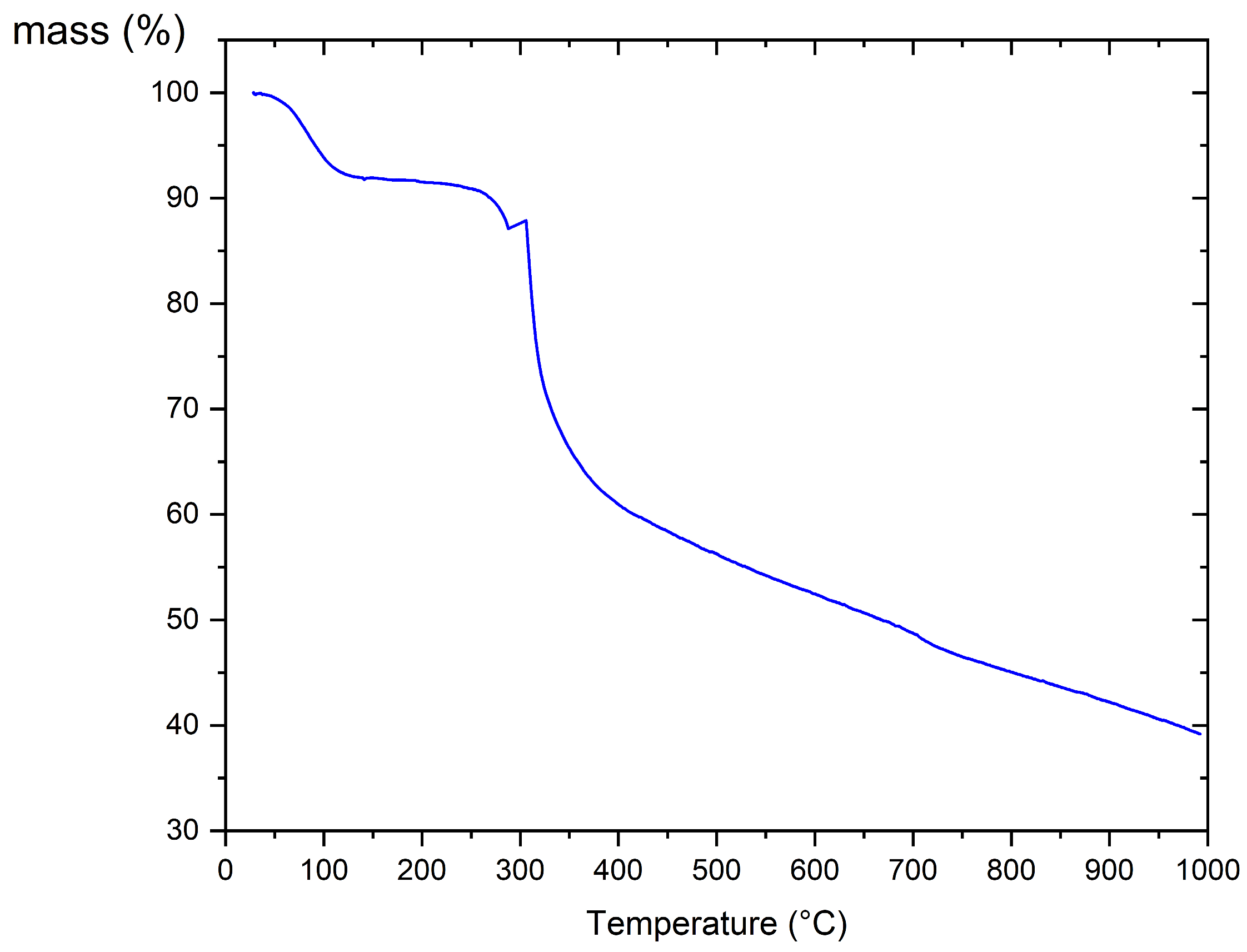
3.1.2. Thermogravimetric Analysis (TGA)

TGA was used to evaluate the thermal stability of the prepared chitosan. The thermogram in Figure 2 shows that the chitosan underwent three main steps of mass loss. As a result of desolvation, the first mass loss started between 28.5 °C and 149.7 °C. At this stage, the chitosan underwent thermal degradation, accompanied by water loss due to the dehydration of polymeric bonds, breakdown of intermolecular interactions, and complete volatilisation. This weight loss, representing approximately 8.1% of the moisture content of the sample, was attributed to the evaporation of residual water, which is in agreement with the conclusions of [37].

The second step was between 287.8 °C and 300 °C, due mainly to the pyrolytic degradation of the polysaccharide chain, in particular, the amine bonds, which require low activation energy. The peak at 300 °C indicates the major decomposition of the chitosan macromolecular structure. This degradation phase results in the release of gases (CO₂, NH₃, H₂O) due to the breaking of chemical bonds. Under certain conditions, volatile or intermediate products may temporarily condense on the sample’s surface before decomposing at higher temperatures, leading to an apparent increase in mass.

The third step (Figure 2), occurring between 300 °C and 400 °C, corresponds to a progressive degradation process resulting in a mass loss of approximately 60.64%. This finding is in agreement with the results reported in [38]. The observed mass loss is attributed to the decomposition of the polymeric structure of chitosan, involving the breakdown of glycosidic bonds and the degradation of functional groups, such as amine and hydroxyl groups.

Above 400 °C, the thermal stability of the chitosan is characterised by two key parameters: the onset temperature of degradation and the extent of mass loss. These factors together provide an indication of the overall thermal stability of the material. This TGA curve confirms that chitosan exhibits good thermal stability within a certain temperature range.

The second step was between 287.8 °C and 291.6 °C, due mainly to the pyrolytic degradation of the polysaccharide chain, in particular, the amine bonds, which require low activation energy. A sudden weight loss of around 12.7% was observed, mainly linked to the emission of CO₂.

Finally, the third step, between 291.7 °C and 992.2 °C, corresponds to progressive degradation, reaching about 60.64% mass loss, in agreement with the results of [38].

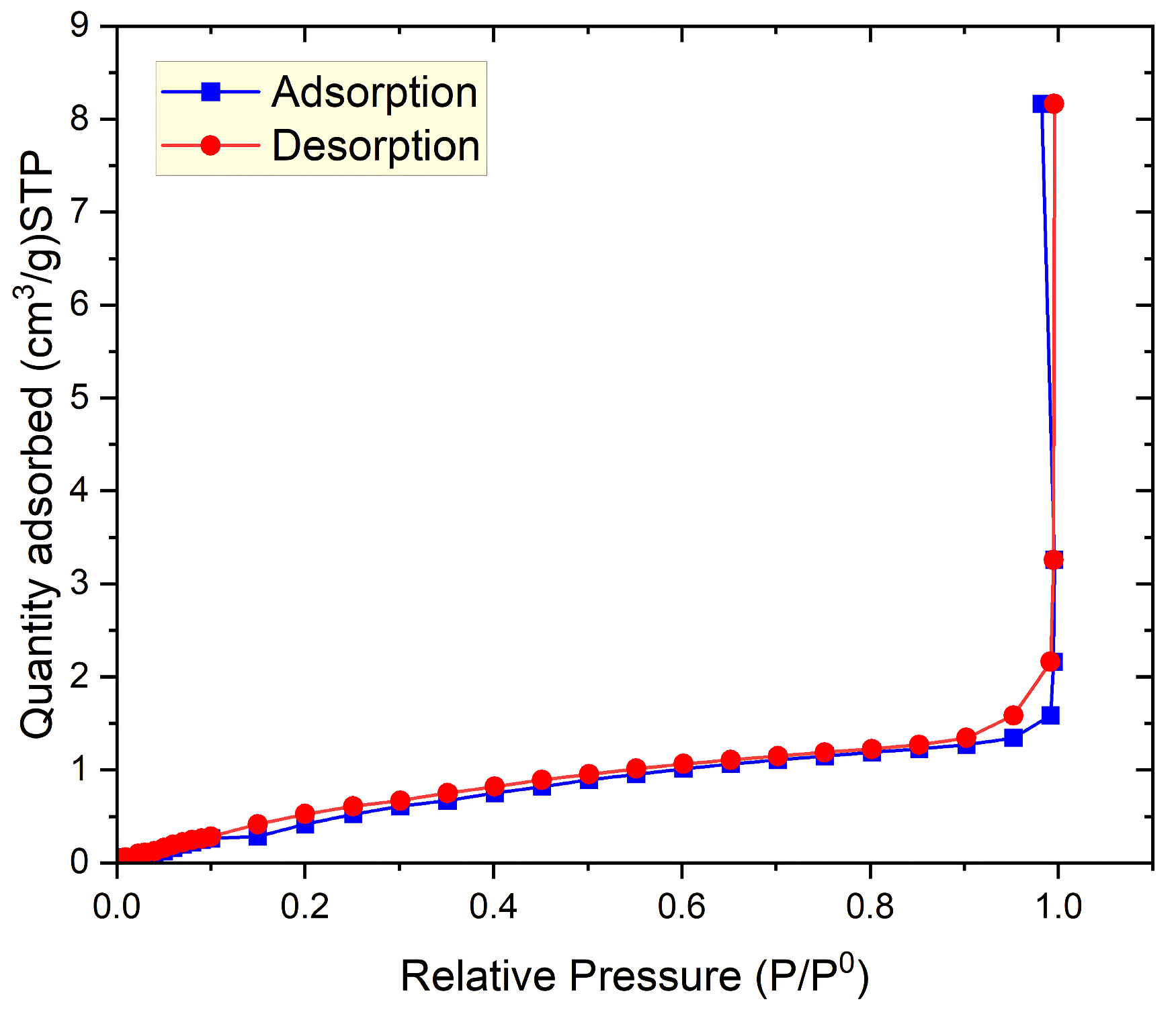
3.1.3. BET Specific Surface Area Analysis

The N₂ adsorption–desorption isotherm for the prepared chitosan is depicted in Figure 3. According to the classifications of IUPAC, it presents a type II isotherm and non-porous or macroporous substances [39]. The prepared chitosan had a specific surface area of 3.24 m²/g and a total volume in the pores of 2.38 × 10⁻³ cm²/g, confirming its non-porous nature. The isotherm formed was a reversible type II isotherm, generally associated with monolayer formation followed by multilayer adsorption

3.1.4. SEM Analysis

Figure 4A shows the SEM image of chitosan. The prepared chitosan was characterized by a rough surface with porous and irregularly distributed agglomerates. Figure 4B clearly shows the irregular morphology and irregular arrangement of the structure formed. The same structure was observed by Mende et al. [40] when analysing the composition of commercial chitosan.

3.2. Adsorption Studies

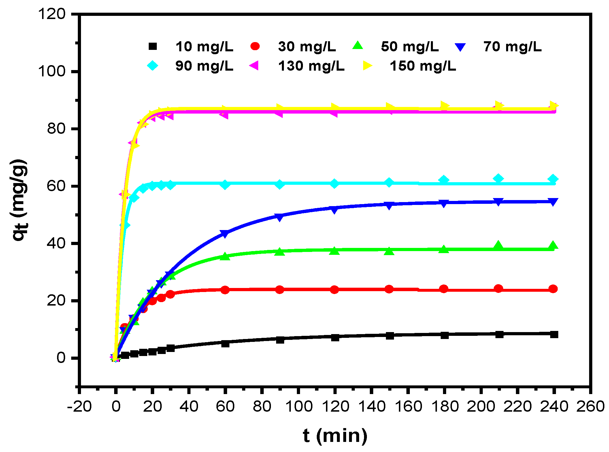
3.2.1. Equilibrium Studies and Adsorption Kinetics Modelling

Two kinetic models were used to analyse the kinetic results for copper adsorption on the prepared chitosan. The adsorption data are identified by using the models, Lagergren’s pseudo-first order (Equation (6a)), and pseudo-second order (Equation (6b)) [41].

$${\mathrm{q}}_{\mathrm{t}}={\mathrm{q}}_{\mathrm{e}}\left(1-{\mathrm{e}}^{-{\mathrm{k}}_1\mathrm{t}}\right)$$

(6a)

$${\mathrm{q}}_{\mathrm{t}}={\displaystyle \frac{{\mathrm{q}}_{\mathrm{e}}^2{ \mathrm{k}}_2 \mathrm{t}}{{\mathrm{q}}_{\mathrm{e}}{\mathrm{k}}_2 \mathrm{t}+1}}$$

(6b)

where:

q_t is the adsorption capacity of copper on chitosan at time t.

k₁ (min⁻¹) is the pseudo-fist-order rate constant.

k₂ (g/mg·min) is the pseudo-second-order rate constant.

q_e: equilibrium value of q.

The nonlinear model was utilized to apply a pseudo-first-order and pseudo-second-order treatment, and the distribution of errors in predicting model parameters was assessed using the chi-squared function (χ²). The model’s fit to the data was calculated using the coefficient of determination (R²); Equations (7) and (8) represent the error functions [42].

$${\mathsf{\chi }}^{2 }={\displaystyle \sum }{\displaystyle \frac{{\left(q_{e,exp}-q_{e,cal}\right)}^2}{q_{e,cal}}}$$

(7)

$${\mathrm{R}}^2=1-{\displaystyle \frac{{\displaystyle \sum }{\left(q_{e,exp}-q_{e,cal}\right)}^2}{{\displaystyle \sum }{\left(q_{e,exp}-q_{mean}\right)}^2}}$$

(8)

where q_e,exp denotes the experimental equilibrium value of q, q_e,cal represents the fitted value of q, and q_e indicates the mean value of the experimental q. A higher value of R² approaching unity implies a better fitting accuracy. When q_e,cal from a model closely aligns with the experimental value q_e,exp, χ² tends towards zero [43].

Figure 5 shows the evolution of the amount of copper ions eliminated by the prepared chitosan until achieving equilibrium, for various copper concentrations. The parameters obtained for the pseudo-first-order and pseudo-second-order models are detailed in

Table 1. The parameters for the first-order and second-order kinetic models used in the removal process of copper at 25 °C are outlined, employing a nonlinearized model.

		Pseudo-First Order				Pseudo-Second Order
C0 (mg/L)	qe (exp)	qe (calc)	K1 (min−1)	R2	χ2	qe (calc)	K2 (min−1)	R2	χ2
10	8.25	8.42 ± 0.12	0.016 ± 6.8 × 10−4	0.99	0.032	10.93 ± 0.25	0.0013 ± 1.11 × 10−4	0.99	0.03
30	24.00	23.69 ± 0.23	0.089 ± 0.004	0.99	0.381	25.23 ± 0.38	0.0058 ± 5.732 × 10−4	0.98	0.65
50	39.00	37.68 ± 0.37	0.046 ± 0.002	0.99	0.854	42.29 ± 0.83	0.00136 ± 1.32 × 10−4	0.99	1.93
70	54.70	54.52 ± 0.44	0.026 ± 7.1 × 10−4	0.99	0.842	65.39 ± 1.32	4.27 × 10−4 ± 3.6 × 10−5	0.99	2.43
90	62.50	60.86 ± 0.29	0.273 ± 0.011	0.99	0.889	62.63 ± 0.47	0.011 ± 0.0012	0.99	1.53
130	87.40	85.85 ± 0.30	0.213 ± 0.005	0.99	0.893	88.98 ± 1.02	0.0053 ± 6.9 × 10−4	0.99	6.72
150	88.10	87.01 ± 0.31	0.201 ± 0.005	0.99	0.967	90.34 ± 0.98	0.0048 ± 5.7 × 10−4	0.99	6.11

.

After comparing the R², χ², and q_e (exp) vs. q_e (calc) values of the two models, we find that there is no significant difference between R², and we have proximity between q_e (exp) vs. q_e (calc) values of the two models, which means that both models provide a good fit to the experimental data.

However, the pseudo-first-order model is the most representative for Cu(II) adsorption on chitosan, as it presents the lowest χ² values, indicating a better fit to the experimental data, especially at low concentrations.

The adsorption of Cu(II) ions follows the pseudo-first-order model at low concentrations, indicating rapid physical adsorption limited by surface diffusion. At high concentrations, the pseudo-second order fits the data better, suggesting strong chemical interactions, such as complexation with the amine groups of chitosan, requiring gradual and balanced adsorption.

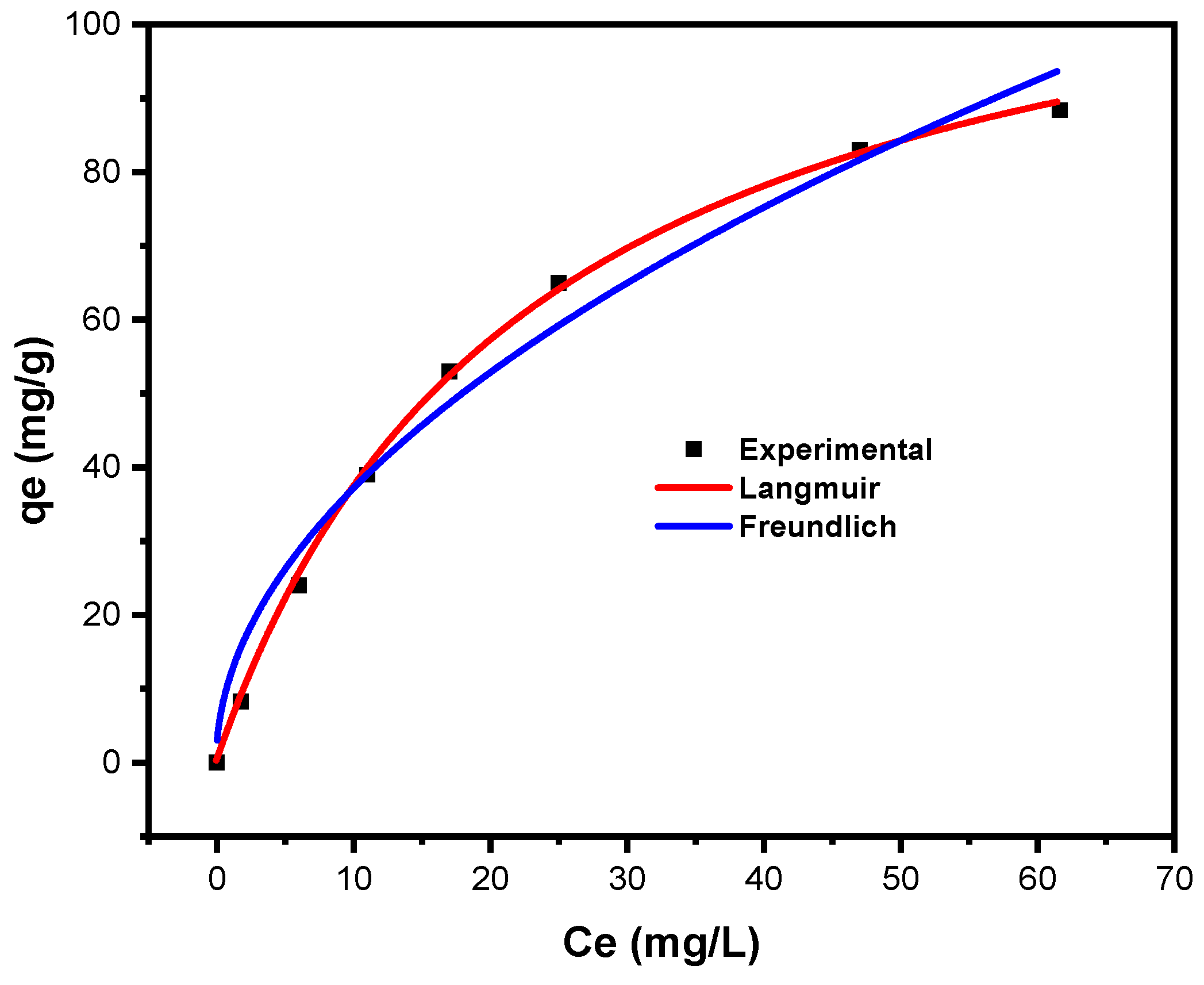
3.2.2. Adsorption Isotherms

Adsorption isotherms elucidate the interplay between adsorbates and adsorbents, crucial for optimizing the utilization of adsorbents. The Langmuir and Freundlich isotherms were assessed for their effectiveness in describing and characterizing the experimental data.

Langmuir Isotherm

The Langmuir isotherm estimates the adsorption of a monolayer onto a surface with a limited number of identical sites. It depends on the assumption that one site is blocked so no further adsorption can happen on it. It assumes monolayer adsorption, meaning that molecules adsorb onto the surface in a single layer and there is no interaction between them. The equation for the Langmuir isotherm is typically represented as [44].

$${\mathrm{q}}_{\mathrm{e}}={\displaystyle \frac{{\mathrm{q}}_{\mathrm{m}}{\mathrm{K}}_{\mathrm{L}}{\mathrm{C}}_{\mathrm{e}}}{1+{\mathrm{K}}_{\mathrm{L}}{\mathrm{C}}_{\mathrm{e}}}}$$

(9)

In this equation, q_max denotes the maximum adsorption capacity of copper per unit mass of adsorbent, achievable when a complete monolayer forms at high Ce, and K_L is a constant reflecting the affinity of the binding sites. The Langmuir isotherm’s key characteristics can be elucidated through a dimensionless constant termed the separation factor, R_L, defined by the equation:

$${\mathrm{R}}_{\mathrm{L}}={\displaystyle \frac{1}{1+{\mathrm{K}}_{\mathrm{L}}{\mathrm{C}}_0}}$$

(10)

where C₀ represents the highest initial concentration of the adsorbate in milligrams per litre (mg/L), while K_L (L/mg) stands for the Langmuir constant. The R_L values serve as indicators of the isotherm’s shape: R_L greater than 1 suggests unfavourable conditions, R_L = 1 demonstrates linearity, R_L = 0 signifies irreversibility, and R_L values between 0 and 1 denote favourability.

Freundlich Isotherm

The Freundlich isotherm is indeed valuable for describing adsorption on heterogeneous surfaces where multiple layers of adsorbate molecules can accumulate. The Freundlich isotherm is expressed through the empirical equation [45]:

$${\mathrm{q}}_{\mathrm{e}}={\mathrm{K}}_{\mathrm{f}}{({\mathrm{C}}_{\mathrm{e}})}^{{\displaystyle \frac{1}{\mathrm{n}}}}$$

(11)

K_f and n represent the Freundlich constants, K_f (mg/g (L/mg)^1/n) signifies the sorbent’s adsorption capacity, while n serves as a constant expressing the favourability of the adsorption process. An n value exceeding 1 indicates favourable adsorption conditions.

The Langmuir and Freundlich constants were determined by the nonlinearized model depicted in Figure 6, with the results reported in

Table 2. Langmuir and Freundlich isotherm parameters for the elimination of copper by chitosan at 25 °C.

Langmuir				Freundlich
qmax (mg/g)	KL (L/mg)	R2	χ2	KF [(mg/g) (mg/L)1/n]	1/n	R2	χ2
123.05 ± 2.27	0.043 ± 0.001	0.999	0.958	11.34 ± 2.12	0.51 ± 0.05	0.971	30.61

.

The constants of the isotherms and their corresponding regression coefficients are presented in Table 2. It is observed that the R² and χ² values were superior for the Langmuir isotherm compared to the Freundlich isotherm, signifying that the Langmuir equation provided a more accurate representation of the adsorption attributed to the even dispersion of active sites across the chitosan’s surface. The value R_L = 0.133 fell within the range of 0 to 1, displaying the favourable adsorption of copper onto chitosan.

The coefficient of determination (R² = 0.999—Table 2) indicates that the Langmuir isotherm provided a good expedient to the results and the monolayer adsorption capacity predicted by this model was q_max= 123.05 mg/g. Q_max of the developed adsorbent aligns with that of other economical adsorbents studied in the existing literature for removing cupric ions, as shown in

Table 3. Comparison of the maximum Langmuir adsorption capacities of chitosan for Cu(II) with other adsorbents.

Materials	pH	Maximum Adsorption Capacity (mg/g)	References
Commercial resins Dowex G-26 and Puromet™ MTS9570	3.5	41.67 and 37.70 mg/g respectively	[46]
synthetic hematite (α-Fe2O3) iron oxide-coated sand (HIOCS)	6	3.93 mg/g	[47]
Ligand of 4-tert-Octyl-4-((phenyl)diazenyl) phenol-silica	4	184.73 mg/g	[48]
Chitosan montmorillonite composite	6	86.95 mg/g	[18]
Kaolinite clay	6	34.12 mg/g	[49]
Natural smectite (NS) and activated carbon (AC)	3.5	26.6 mg/g and 36.6 mg/g respectively	[50]
NaOH-treated rice husk	6	3.75 mg/g	[51]
Chitosan using crab shells from nylon shrimps	2.5 4.5	135 mg/g 238 mg/g	[52]
Chitosan from partially deacetylated prawn shell	6	16.9 mg/g	[53]
Shrimp carapace-derived chitosan	6.5	123 mg/g	This study

. This suggests that shrimp shell-derived chitosan stands competitively alongside several other materials documented in the prior research.

Table 3 indicates that most of the adsorption capacities of cupric ions by different adsorbents are lower than those observed in this study, except the ligand of 4-tert-octyl-4-((phenyl)diazenyl) phenol-silica, which displays a higher adsorption capacity, confirming that chelation compounds possess a strong ability to remove cupric ions.

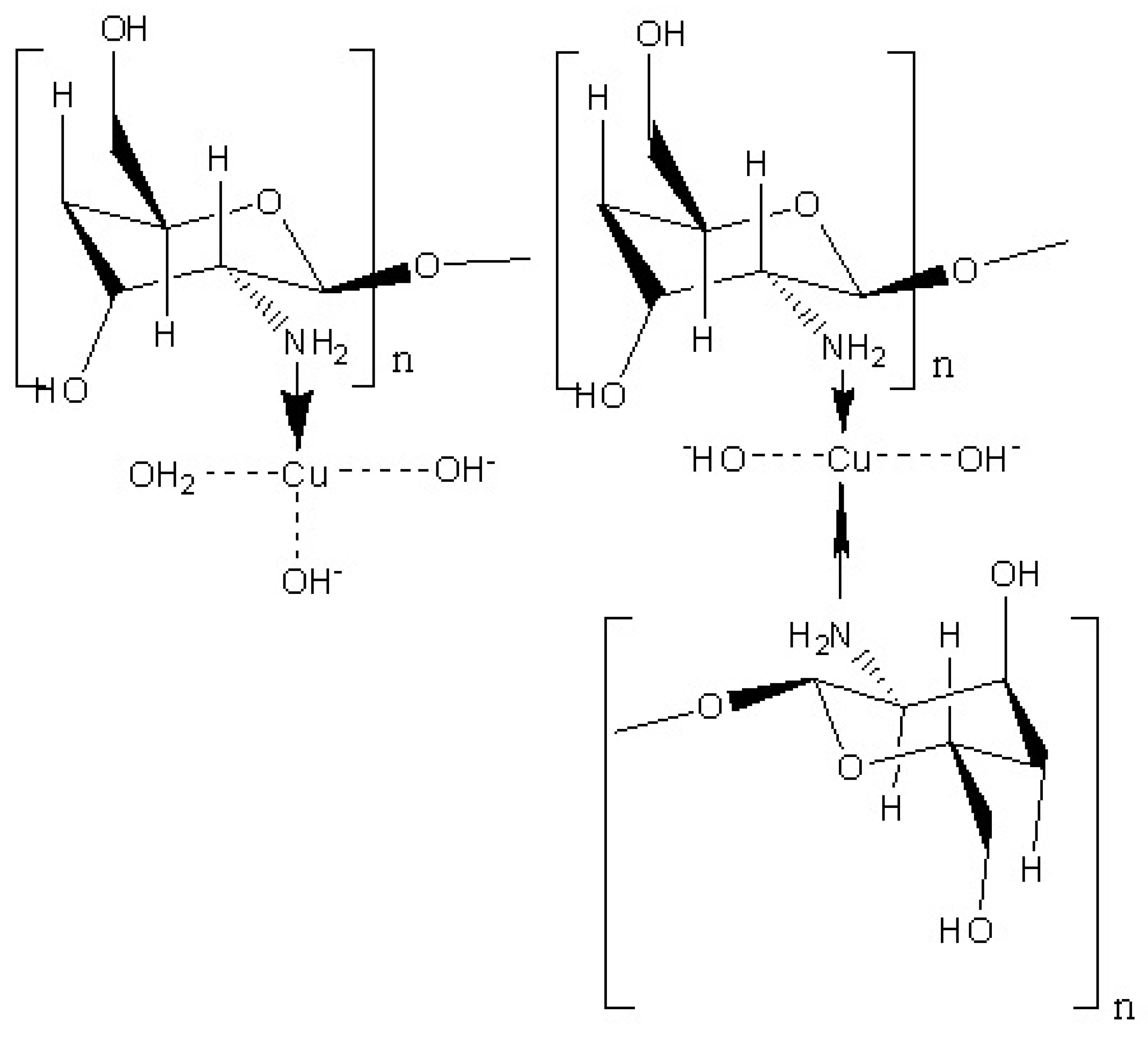
3.2.3. Mechanism of Metal Ion Removal by Chitosan

The high capacity of chitosan to remove copper ions can be explained by the interaction of two simultaneous phenomena: the adsorption of copper ions onto the chitosan’s surface and the complexation of chitosan with metals via chelation and metal–ligand interactions. Figure 7 shows two types of coordination complexes [54] that can be formed: these structures, labelled type I and type II, illustrate different modes of copper coordination with chitosan, highlighting, in particular, the interaction between copper ions (Cu²⁺) and amino groups (–NH₂) in chitosan. The type I complex shows a copper ion coordinated to two hydroxide ions (OH⁻) and a water molecule (H₂O), forming a structure in which the chitosan binds the copper ion to the amino group of the polymer. In the type II complex, two amino groups coordinate with the Cu²⁺ and two hydroxide ions, forming a more stable configuration with the chitosan. Due to the unique properties of chitosan and its ability to chelate metal ions, such as copper, these complexes are of particular interest for various applications, such as catalysts, antimicrobial agents, or environmental remediation [55,56].

3.3. Optimization and Modelling via the Response Surface Methodology (RSM) Using the Experimental Design (DOE)

3.3.1. Analysis of the Results Obtained Through Planning by the Experimental Design (DOE)

This study investigates the effects of the operating parameters’ pH, chitosan mass, copper solution concentration, contact time, reaction temperature, and ionic strength (NaCl) on the adsorption of copper ions from the solution by chitosan synthesized from shrimp shells. A central design of the composite was used as part of the design of experiments (DOE) methodology for this study. Six input factors were considered, each factor having three levels, with the output variable (response) being the adsorption capacity and percentage elimination of Cu²⁺ on the prepared chitosan.

Table 4. Factors with their actual and coded levels.

No.	Variable	Name	Variable Level
			−1	0	+1
01	X1	pH	4	7	10
02	X2	T (°C)	25	35	45
03	X3	Metal concentration (mg/L)	20	70	120
04	X4	t (min)	30	140	250
05	X5	Adsorbent concentration S/L (g/L)	0.3	1.4	2.5
06	X6	NaCl (mol/L)	0.1	0.3	0.5

lists the factors studied with their actual and coded levels. The combination of these parameters, according to the central composite design, led to the experimental execution of 46 manipulations, with the results summarised in

Table 5. The actual central composite design (CC) matrix of experiments for copper removal.

Run	pH	T (°C)	Metal Concentration (mg/L)	t (min)	Adsorbent Concentration (g/L)	NaCl (mol/L)	Observed Adsorption Capacity (mg/g)	Predicted Adsorption Capacity (mg/g)	Residual Adsorption Capacity (mg/g)	Observed Removal (%)
1	7	35	70	140	2.5	0.3	27.74	30.046	−2.306	99.07
2	4	25	120	250	0.3	0.5	359.08	365.584	−6.504	89.77
3	10	45	20	30	0.3	0.5	64.08	67.686	−3.606	69.12
4	7	35	70	140	1.4	0.5	49.89	47.494	2.395	99.79
5	7	35	20	140	1.4	0.3	14.17	6.548	7.621	99.2
6	7	35	70	140	0.3	0.3	231.19	225.592	5.597	99.08
7	10	45	20	30	2.5	0.1	6.85	0.551	6.298	85.62
8	10	45	20	250	2.5	0.5	7.71	4.512	3.197	96.37
9	7	25	70	140	1.4	0.3	49.37	47.603	1.766	98.75
10	4	35	70	140	1.4	0.3	49.72	43.935	5.784	99.44
11	10	25	120	250	0.3	0.1	396.22	393.957	2.262	99.05
12	4	25	120	250	2.5	0.1	47.99	44.589	3.400	99.98
13	10	45	120	250	2.5	0.1	47.87	51.894	−4.024	99.73
14	4	45	120	30	2.5	0.1	47.69	43.100	4.589	99.36
15	10	45	20	250	0.3	0.1	66.61	71.827	−5.217	99.91
16	4	45	20	250	2.5	0.1	7.25	14.079	−6.829	90.62
17	10	25	120	30	2.5	0.1	47.77	51.995	−4.225	99.53
18	10	25	20	250	2.5	0.1	7.78	0.935	6.844	97.33
19	10	25	20	30	2.5	0.5	7.99	8.983	−0.993	99.91
20	4	45	120	250	2.5	0.5	47.99	44.726	3.263	99.98
21	7	35	70	250	1.4	0.3	49.75	48.662	1.0871	99.5
22	10	35	70	140	1.4	0.3	49.33	51.823	−2.493	98.67
23	4	25	20	250	0.3	0.1	65.69	63.082	2.607	98.54
24	4	25	20	250	2.5	0.5	7.95	11.307	−3.357	99.41
25	7	35	70	140	1.4	0.3	49.5	57.947	−8.447	99
26	4	45	20	30	0.3	0.1	60	59.143	0.856	90
27	4	25	120	30	2.5	0.5	47.93	42.917	5.012	99.85
28	10	25	20	30	0.3	0.1	66.61	70.079	−3.469	99.91
29	10	25	120	250	2.5	0.5	47.8	48.861	−1.061	99.59
30	10	45	120	30	2.5	0.5	47.84	50.652	−2.812	99.68
31	7	35	70	30	1.4	0.3	49.44	47.236	2.203	98.89
32	10	45	120	30	0.3	0.1	396.08	392.928	3.151	99.02
33	7	45	70	140	1.4	0.3	49.48	47.955	1.524	98.97
34	4	45	120	30	0.3	0.5	356.77	363.820	−7.050	89.19
35	7	35	70	140	1.4	0.3	49.94	57.947	−8.007	99.88
36	7	35	120	140	1.4	0.3	180	184.330	−4.330	99.79
37	10	45	120	250	0.3	0.5	398.05	393.729	4.320	99.51
38	4	25	120	30	0.3	0.1	366.25	369.653	−3.403	91.56
39	10	25	120	30	0.3	0.5	398.66	392.035	6.6242	99.66
40	4	25	20	30	2.5	0.1	7.69	12.216	−4.5260	96.12
41	4	45	120	250	0.3	0.1	378.47	377.681	0.788	94.61
42	4	45	20	30	2.5	0.5	7.72	10.188	−2.468	96.58
43	7	35	70	140	1.4	0.1	49.87	48.974	0.895	99.75
44	4	45	20	250	0.3	0.5	66.19	62.170	4.019	99.29
45	10	25	20	250	0.3	0.5	63.55	68.345	−4.795	95.33
46	4	25	20	30	0.3	0.5	62.33	58.511	3.818	93.5

.

Based on the experimental results presented in the Table 5 and prior to conducting a statistical analysis, it was noticed that the removal efficiency of cupric ions via adsorption and chelation with chitosan ranged from 85.62% to 99.98%, irrespective of the levels of factors affecting the adsorption and chelation. Additionally, the maximum number of cupric ions removed by chitosan varied between 356.77 mg/g and 396.22 mg/g for a copper solution concentration of 120 mg/L and a minimum chitosan concentration of 0.3 g/L, regardless of the values of other influencing factors.

3.3.2. Analysis of Variance (ANOVA)

Two key aspects can be investigated when analysing the experimental model. The first is the significance index (the p-value). According to Goupy and Creighton [57], a p-value of less than 0.05 indicates a significant factor, a p-value of less than 0.01 indicates a very significant factor, and a p-value of less than 0.001 indicates a highly significant factor. The second aspect is the random variability of the response. When a response at the same point is detected many times, the results may vary slightly. This variation, known as the experimental error, is denoted by e (where e < 10 indicates an insignificant error) [57]. As shown in Figure 8, the obtained model was highly significant (p < 0.0001) and the predicted adsorption capacity was in close agreement with the corresponding experimental results. Its points were closely clustered around the model line, demonstrating the vigorous model with an R² value of 1, indicating an excellent fit to the real model. In addition, the root mean square error (RMSE) was 7.0543, less than 10%, further validating the accuracy of the model [30].

The understanding of the factors and their interactions was evaluated using the ANOVA feature in JMP software 13.2. The data, depicted in

Table 6. ANOVA for the data appropriate to the response of the surface model.

Factor	DF	Sum of Squares	F-Value	p-Value
Adsorbent concentration (X5)	1	325,022.68	6531.354	<0.0001
Metal concentration (X3)	1	268,654.02	5398.622	<0.0001
Metal concentration × Adsorbent concentration (X3X5)	1	152,984.70	3074.238	<0.0001
Adsorbent concentration × Adsorbent concentration (X5X5)	1	11,609.75	233.2988	<0.0001
Metal concentration × Metal concentration (X3X3)	1	3342.72	67.1721	<0.0001
pH × Adsorbent concentration (X1X5)	1	575.28	11.5604	0.0032
pH (X1)	1	528.83	10.6268	0.0043
pH× Metal concentration (X1X3)	1	463.30	9.3100	0.0069
T × T (X2X2)	1	245.83	4.9400	0.0393
pH × pH (X1X1)	1	241.02	4.8433	0.0410
t × t (X4X4)	1	237.68	4.7762	0.0423
NaCl × NaCl (X6X6)	1	224.32	4.5077	0.0479

, exhibit that the adsorbent concentration (X5) has a highly significant effect, with p < 0.0001 and F = 6531.354. This was followed by the metal concentration (X3), which also had a highly significant effect with p < 0.0001 and F = 5398.622. The pH (X1) had a lower effect, with p = 0.0043 and F = 10.626. The other factors are not signified on the adsorption of copper onto the chitosan. Table 6 also highlights the highly significant interaction between X3 and X5 (X3X5), as well as a moderate interaction between X1 and X5 (X1X5). The regression analysis demonstrated that the quadratic terms X₅² and X₃² were very highly significant, while the terms X₁², X₂², X₄², and X₆² were also significant.

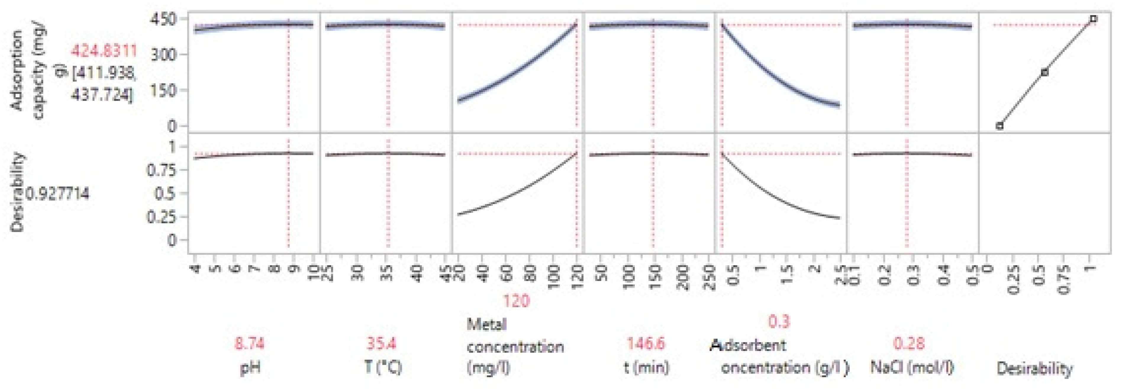
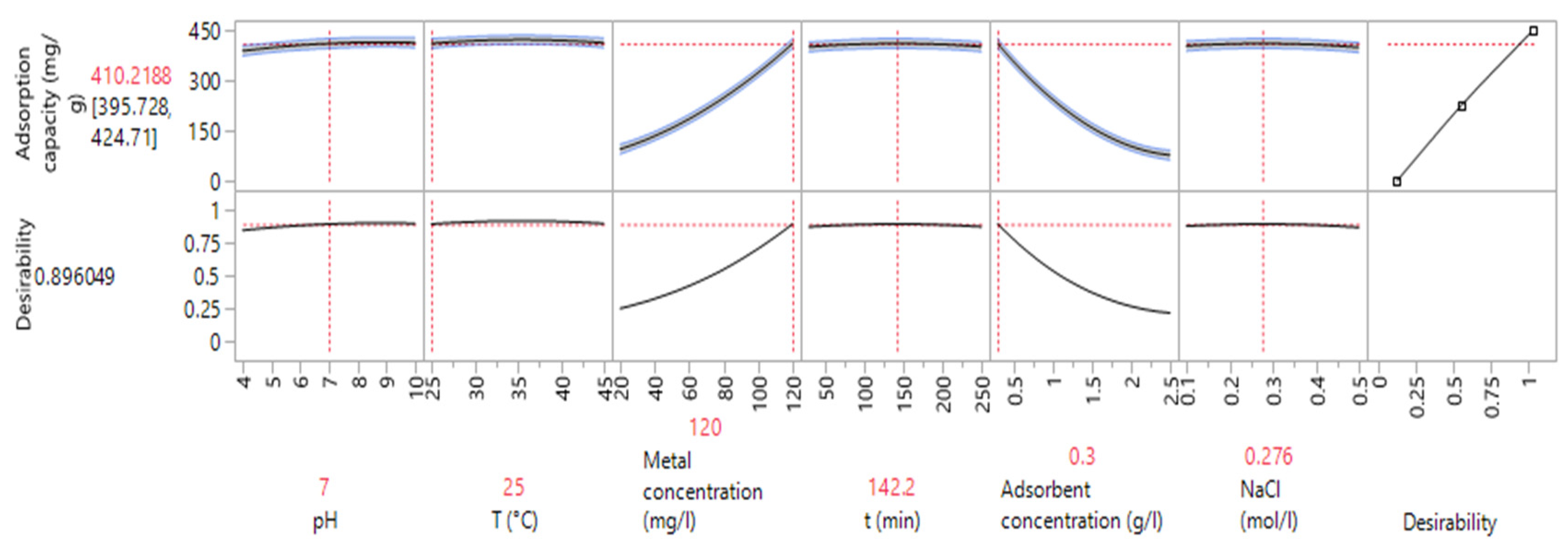
3.3.3. Optimization of the Values of the Variables

To determine the optimal values of the variables that maximize the adsorption capacity of copper ions by chitosan, a diagram of optimization was formed through the maximum desirability function (D = 1) in JMP^® Pro statistical software version 13.2.1. In the diagram, the responsibility of the six factors was shown for each one in separate columns. The factor response is represented by the red dashed horizontal lines while the factor values are characterized by the vertical lines.

In Figure 9, it can be seen that the simulation was adjusted to maximize the adsorption capacity (mg/g), identifying the statistical sweet spot for q_max = 424.83 mg/g and d = 0.927. These optimal conditions corresponded to a metal concentration of 120 mg/L, an adsorbent concentration of 0.3 g/L, a pH of 8.74, a temperature of 35.4 °C, a contact time of 146.6 min, and [NaCl] = 0.28 mol/L.

As shown in the ANOVA table, the pH and temperature do not have an effect on the adsorption of copper ions onto the chitosan. Given that, it is always preferable to work in natural conditions for economic and industrial reasons, and hence the q_max at a neutral pH and ambient temperature using the maximum desirability function was determined (Figure 10).

At pH = 7, room temperature (25 °C), and in 120 mg/L of a copper solution using 0.3 g/L of chitosan, with a NaCl concentration of 0.276 mol/L in a batch mode over 142.2 min, it is possible to achieve q_max = 410.22 mg/g for copper ions onto the prepared chitosan (Figure 10).

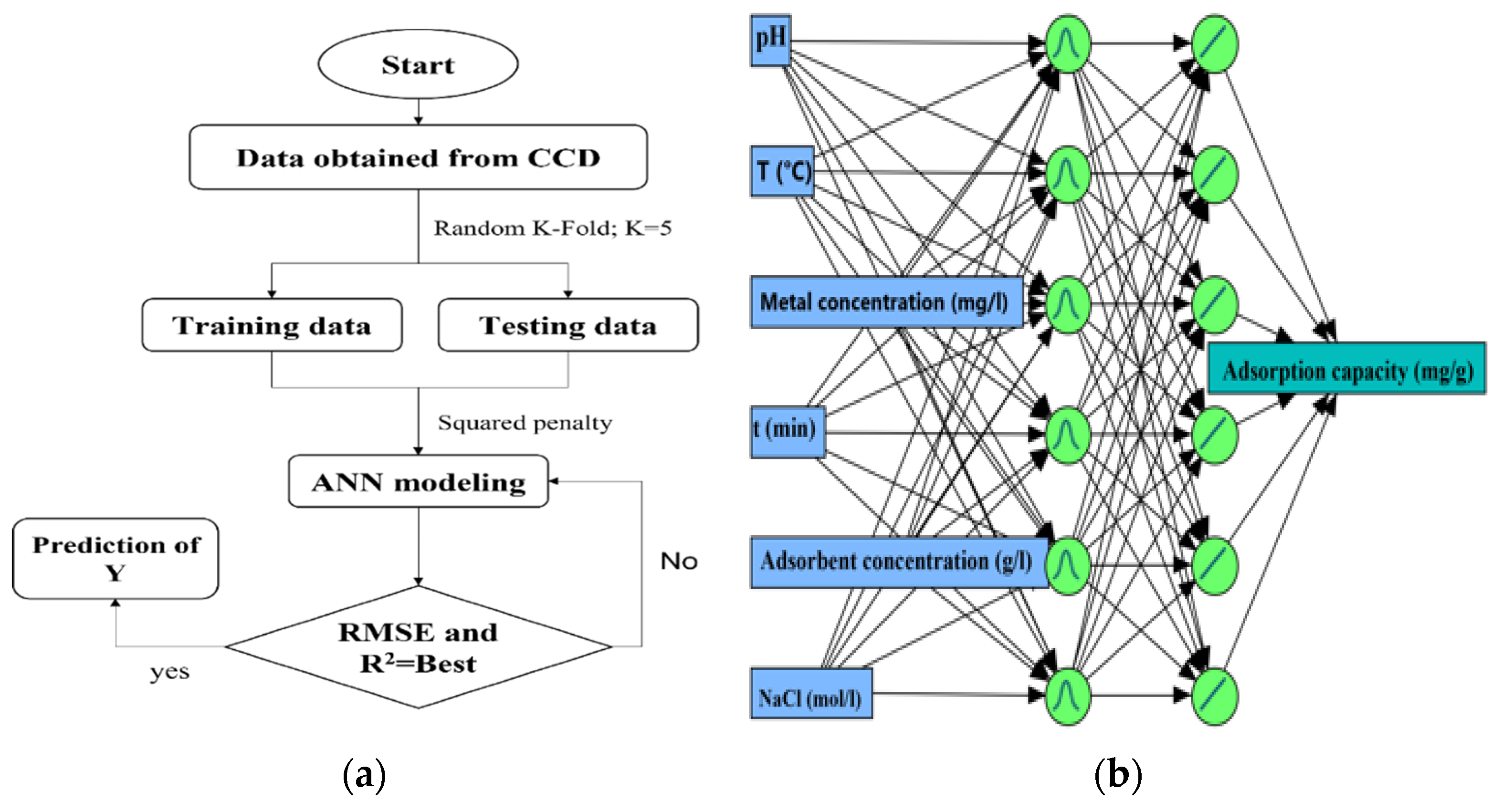
3.4. Artificial Neural Networks (ANNs)

3.4.1. Artificial Neural Networking Strategy

ANNs are a prominent model commonly used in machine learning, inspired by the intricate information processing observed in the human brain. This innovative approach mimics the interconnected neural clusters found in biological systems and has proven to be a powerful modelling technique for dealing with complex nonlinear processes. In this study, an ANN was used to predict the relationship between the specified input variables (X1, X2, X3, X4, X5, and X6) and adsorption capacity. The architecture of the ANN model included an input layer consisting of X1, X2, X3, X4, X5, and X6, an output layer representing the adsorption capacity, and two intermediate hidden layers integrating both linear and Gaussian functions. This ANN model was developed based on the empirical data from the CCD, as shown in Figure 11. The adsorption capacity dataset (Table 5) was randomly partitioned using the random K-fold method to create subsets for training and validation purposes. This approach ensures a robust training regime for the ANN, facilitating its proficiency in predicting the adsorption capacity under different input conditions. In addition, the squared penalty method was used to overfit the data using Equation (12).

$$Penalty method=\lambda \mathrm{p}\left(B_i\right)$$

(12)

$$\mathrm{p}\left(B_i\right)={\displaystyle \sum }{B}_i^2$$

(13)

where $\lambda$ is the penalty parameter, and $\mathrm{p}\left(B_i\right)={\displaystyle \sum }{B}_i^2$ is the penalty function (squared penalty).

The prediction accuracy of the ANN model for TPC and TFC was calculated by using R² and RMSE, log likelihood, mean absolute deviation (MAD), and sum of squared error (SSE).

The adsorption capacity predicted by the ANN and the prediction accuracy of the ANN model are clearly illustrated in

Table 7. Prediction accuracy of the ANN model.

Measures	Training	Validation
R2	0.999	0.998
RASE	0.76	5.37
MAD	0.53	3.85
Log likelihood	42.44	27.89
SSE	21.48	259.58
Sum of frequency	37	9

Notes: MAD: mean absolute deviation, RASE: root average squared error, and SSE: sum of square error.

and Figure 12.

3.4.2. Optimization of Variable Values and Maximization of Adsorption Capacity Using ANNs

In order to obtain the optimum values of the variables for the maximum removal of copper ions on the prepared chitosan, optimization using the neural analysis provided by JMP software was carried out. This optimization was carried out using two layers, Gaussian and linear, as shown in Figure 13.

The optimal conditions were found to be [metal] = 107 mg/L, an adsorbent concentration of 0.3 g/L, pH = 9.4, at 45 °C, a contact time of 250 min, and a NaCl concentration of 0.4 mol/L. Under these conditions, the adsorption capacity of copper ions onto the prepared chitosan reached 468 mg/g.

3.4.3. Mathematical Modelling by ANNs

The parameter evaluates of ANNs proposed by JMP was used to determine the relationships between the six factors and experimental response for the adsorption capacity (mg/g). Based on these parameters, the adsorption of copper ions onto chitosan derived from shrimp shells can be predicted using Equation (14).

$$\begin{array}{cc}Adsorption \hfill & capacity \left(\mathrm{mg}/\mathrm{g}\right)\hfill \\ & =54.70-44.60 H_{1\left(1\right)}+423.57 H_{1\left(2\right)}\pm 244.25 H_{1\left(3\right)}\hfill \\ & -273.91 H_{1\left(4\right)}-217.68 H_{1\left(5\right)}-74.23 H_{1\left(6\right)}\hfill \end{array}$$

(14)

where H_1(n), is the first hidden layer (linear), and n is the number of nodes.

3.4.4. RSM Evolution by ANNs and Effects of Parameters

Figure 14a shows the response surface of the adsorption capacity as a function of metal (copper) concentration (X3) and adsorbent (chitosan) concentration (X5). The graph exhibits a negative interaction between these two factors, with the adsorption capacity reaching 450 mg/g at the maximum metal concentration and the minimum adsorbent concentration. When the factors X1 and X5 interacted, a maximum adsorbed amount of 250 mg/g was observed at the minimum value of X5, regardless of the value of X1. This confirms that X1 has no representative effect on the adsorption of copper by chitosan (Figure 14b). A similar observation was made for the response surface as a function of X3 and X4. Since X4 had no significant effect on the adsorption and X3 was a highly significant factor, a significant adsorption value of 300 mg/g was achieved for a concentration of 100 mg/L of copper ions (X3), irrespective of the value of X4 (Figure 14c). The response surface as a function of factors X1 and X6 (Figure 14d) showed a low maximum adsorbed amount of 56 mg/g at [NaCl] = 0.1 mol/L and a basic pH of around 8 during their interaction, indicating no significant effect of these two variables.

3.5. Thermodynamic Studies

The energy changes and the spontaneous nature of the adsorption were obtained by a thermodynamic study. In this work, the thermodynamics of the adsorption process was studied at five different temperatures ranging from 298.18 K to 338.15 K. Thermodynamic parameters, such as the Gibbs free energy change (ΔG⁰), enthalpy (ΔH⁰), and entropy (ΔS⁰), were determined based on the Van’t Hoff Equation (15) [58,59].

$$\Delta {\mathrm{G}}^0=-\mathrm{RT} \ln ({\mathrm{K}}_{\mathrm{L}}^0)$$

(15)

Here, R = 8.314 J/mol is the universal gas constant, T is the absolute temperature in Kelvin (K), and K_L⁰ is the dimensionless thermodynamic Langmuir constant for the adsorption process. K_L⁰ is derived from the Langmuir constant K_L (L/mg) after converting all the concentrations to their molar form and assuming a standard state concentration of C₀ = 1 mol/L (Equation (16)) [59].

$${\mathrm{K}}_{\mathrm{L}}^0={\mathrm{K}}_{\mathrm{L}}\left({\displaystyle \frac{\mathrm{L}}{\mathrm{mg}}}\right)·1000\left({\displaystyle \frac{\mathrm{mg}}{\mathrm{g}}}\right)·{\mathrm{M}}_{\mathrm{Cu}}\left({\displaystyle \frac{\mathrm{g}}{\mathrm{mol}}}\right)·{\mathrm{C}}^0\left({\displaystyle \frac{\mathrm{mol}}{\mathrm{L}}}\right)$$

(16)

where M_Cu = 63.546 g/mol, representing the molar mass of copper, and the factor of 1000 is used to convert grams to milligrams. ΔH⁰ and entropy ΔS⁰ parameters were predicted using Equations (17) and (18):

$$\Delta {\mathrm{G}}^0=\Delta {\mathrm{H}}^0-\mathrm{T}\Delta {\mathrm{S}}^0$$

(17)

$$\ln {\mathrm{K}}_{\mathrm{L}}^0=(\Delta {\mathrm{S}}^0/\mathrm{R})-(\Delta {\mathrm{H}}^0/\mathrm{RT})$$

(18)

The plot of lnK_L⁰ against 1/T resulted in a straight line, from which (ΔH⁰) (kJ/mol) and (ΔS⁰) (J/mol·K) were assessed using the intercept and slope of the Van ‘t Hoff plot, respectively. The results of the thermodynamic study are summarized in

Table 8. Thermodynamic parameters for copper ions’ adsorption by chitosan.

T (°K)	KL (L/mg)	KL0	Ln KL0	∆G0 (kJ/mol)	∆H0 (kJ/mol)	∆S0 (J/mol·K)
298.15	0.00044	27.98	3.33	−8.25
308.15	0.00034	22.01	3.09	−7.92
318.15	0.00026	16.69	2.81	−7.44	−21.78	−45.14
328.15	0.00021	13.25	2.58	−7.05
338.15	0.00015	09.86	2.28	−6.43

. The negative (ΔG⁰) values show that the adsorption is favourable and spontaneous, while the negative (ΔH⁰) values signify that the adsorption is exothermic.

4. Conclusions

The prepared chitosan was employed to remove Cu²⁺ ions from an aqueous solution using the batch adsorption method. Under optimized conditions (pH = 6.5, temperature = 25 °C, and chitosan concentration = 1 g/L), the adsorption capacity of Cu(II) reached approximately 89 mg/g. Kinetic studies revealed that both nonlinear pseudo-first-order and pseudo-second-order models effectively described the adsorption process, with the pseudo-first-order model providing a better fit at lower Cu(II) concentrations.

Equilibrium adsorption data were analysed using the Langmuir and Freundlich isotherm models. The Langmuir model demonstrated a superior fit, indicating monolayer adsorption with a maximum capacity of 123 mg/g under the same conditions.

To further investigate the adsorption process, the effects of key parameters, such as initial Cu²⁺ concentration, pH, chitosan concentration (S/L), temperature, contact time, and NaCl concentration, were systematically evaluated using the central composite design (CCD) and response surface methodology (RSM). Analysis of variance (ANOVA) identified the initial Cu²⁺ concentration and chitosan dosage (S/L) as the most significant factors influencing the adsorption efficiency, while the other parameters showed a negligible impact.

Artificial neural network (ANN) modelling was also applied to predict the adsorption behaviour, revealing a remarkable adsorption capacity of 467.983 mg/g under optimized conditions. Additionally, thermodynamic studies confirmed that the adsorption process was spontaneous and exothermic, further supporting the feasibility of chitosan as an effective adsorbent for Cu²⁺ removal.

References

1. Nieder, R.; Benbi, D.K. Potentially toxic elements in the environment–a review of sources, sinks, pathways and mitigation measures. Rev. Environ. Health 2024, 39, 561–575. [Google Scholar] [CrossRef] [PubMed]
2. Ali, H.; Khan, E. What are heavy metals? Long-standing controversy over the scientific use of the term ‘heavy metals’–proposal of a comprehensive definition. Toxicol. Environ. Chem. 2018, 100, 6–19. [Google Scholar] [CrossRef]
3. Chai, W.S.; Cheun, J.Y.; Kumar, P.S.; Mubashir, M.; Majeed, Z.; Banat, F.; Ho, S.-H.; Show, P.L. A review on conventional and novel materials towards heavy metal adsorption in wastewater treatment application. J. Clean. Prod. 2021, 296, 126589. [Google Scholar] [CrossRef]
4. Maskawat Marjub, M.; Rahman, N.; Dafader, N.C.; Tuhen, F.S.; Sultana, S.; Ahmed, F.T. Acrylic acid-chitosan blend hydrogel: A novel polymer adsorbent for adsorption of lead (II) and copper (II) ions from wastewater. J. Polym. Eng. 2019, 39, 883–891. [Google Scholar] [CrossRef]
5. Bawa, U. Heavy metals concentration in food crops irrigated with pesticides and their associated human health risks in Paki, Kaduna State, Nigeria. Cogent Food Agric. 2023, 9, 2191889. [Google Scholar] [CrossRef]
6. Yang, J.; Ma, S.; Zhou, J.; Song, Y.; Li, F. Heavy metal contamination in soils and vegetables and health risk assessment of inhabitants in Daye, China. J. Int. Med. Res. 2018, 46, 3374–3387. [Google Scholar] [CrossRef]
7. Vilas–Boas, J.A.; Cardoso, S.J.; Senra, M.V.X.; Rico, A.; Dias, R.J.P. Ciliates as model organisms for the ecotoxicological risk assessment of heavy metals: A meta–analysis. Ecotoxicol. Environ. Saf. 2020, 199, 110669. [Google Scholar] [CrossRef]
8. Alam, M.; Rohani, M.F.; Hossain, M.S. Heavy metals accumulation in some important fish species cultured in commercial fish farm of Natore, Bangladesh and possible health risk evaluation. Emerg. Contam. 2023, 9, 100254. [Google Scholar] [CrossRef]
9. Singh, A.; Pal, D.B.; Mohammad, A.; Alhazmi, A.; Haque, S.; Yoon, T.; Srivastava, N.; Gupta, V.K. Biological remediation technologies for dyes and heavy metals in wastewater treatment: New insight. Bioresour. Technol. 2022, 343, 126154. [Google Scholar] [CrossRef]
10. Browner, C.M. Development Document for Effluent Limitations Guidelines and Standards for the Centralized Waste Treatment Industry: Final; US Environmental Protection Agency, Office of Water: Washington, DC, USA, 2000; Volume 2.
11. Organisation Mondiale de la Santé. Directives Sur la Qualité de L’eau de Boisson: Quatrième Edition Intégrant le Premier Additif, 4th ed.; Organisation Mondiale de la Santé: Geneva, Switzerland, 2017.
12. Komárek, M.; Čadková, E.; Chrastný, V.; Bordas, F.; Bollinger, J.-C. Contamination of vineyard soils with fungicides: A review of environmental and toxicological aspects. Environ. Int. 2010, 36, 138–151. [Google Scholar] [CrossRef]
13. Leng, S.; Guo, X.; Ma, N.; Li, B.; Zhang, X.; Ding, Y.; Zhao, L. Bottom-Up Synthesis of an Oligo-dithiocarbamate Chelating Precipitant and Its Direct Removal of Complexed Heavy Metals from Acidic Wastewater. ACS ES&T Water 2023, 3, 2581–2589. [Google Scholar]
14. Doyo, A.N.; Kumar, R.; Barakat, M.A. Recent advances in cellulose, chitosan, and alginate based biopolymeric composites for adsorption of heavy metals from wastewater. J. Taiwan Inst. Chem. Eng. 2023, 151, 105095. [Google Scholar] [CrossRef]
15. Ozcan, A.S.; Gök, O.; Ozcan, A. Adsorption of lead(II) ions onto 8-hydroxy quinoline-immobilized bentonite. J. Hazard. Mater. 2009, 161, 499–509. [Google Scholar] [CrossRef]
16. Cheikh, S.; Imessaoudene, A.; Bollinger, J.-C.; Manseri, A.; Bouzaza, A.; Hadadi, A.; Hamri, N.; Amrane, A.; Mouni, L. Adsorption behavior and mechanisms of the emerging antibiotic pollutant norfloxacin on eco-friendly and low-cost hydroxyapatite: Integrated experimental and response surface methodology optimized adsorption process. J. Mol. Liq. 2023, 392, 123424. [Google Scholar] [CrossRef]
17. Bouchelkia, N.; Mouni, L.; Belkhiri, L.; Bouzaza, A.; Bollinger, J.C.; Madani, K.; Dahmoune, F. Removal of lead (II) from water using activated carbon developed from jujube stones, a low-cost sorbent. Sep. Sci. Technol. 2016, 51, 1645–1653. [Google Scholar] [CrossRef]
18. Ye, X.; Shang, S.; Zhao, Y.; Cui, S.; Zhong, Y.; Huang, L. Ultra-efficient adsorption of copper ions in chitosan–montmorillonite composite aerogel at wastewater treatment. Cellulose 2021, 28, 7201–7212. [Google Scholar] [CrossRef]
19. Ahmed, M.A.; Ahmed, M.A.; Mohamed, A.A. Synthesis, characterization and application of chitosan/graphene oxide/copper ferrite nanocomposite for the adsorptive removal of anionic and cationic dyes from wastewater. RSC Adv. 2023, 13, 5337–5352. [Google Scholar] [CrossRef]
20. Javad Sajjadi Shourije, S.M.; Dehghan, P.; Bahrololoom, M.E.; Cobley, A.J.; Vitry, V.; Azar, G.T.P.; Kamyab, H.; Mesbah, M. Using fish scales as a new biosorbent for adsorption of nickel and copper ions from wastewater and investigating the effects of electric and magnetic fields on the adsorption process. Chemosphere 2023, 317, 137829. [Google Scholar] [CrossRef]
21. Fundji, W.N.; Igberase, E.; Osifo, P.; Kabuba, J. Modification of chitosan with cellulose and gelatin for the removal of Cu2+, Fe2+, and Pb2+ from oily wastewater. Can. J. Chem. Eng. 2023, 101, 4711–4730. [Google Scholar] [CrossRef]
22. Roosen, J.; Van Roosendael, S.; Borra, C.R.; Van Gerven, T.; Mullens, S.; Binnemans, K. Recovery of scandium from leachates of Greek bauxite residue by adsorption on functionalized chitosan-silica hybrid materials. Green Chem. Int. J. Green Chem. Resour. GC 2016, 18, 2005–2013. [Google Scholar] [CrossRef]
23. Teng, D.; Jin, P.; Guo, W.; Liu, J.; Wang, W.; Li, P.; Cao, Y.; Zhang, L.; Zhang, Y. Recyclable Magnetic Iron Immobilized onto Chitosan with Bridging Cu Ion for the Enhanced Adsorption of Methyl Orange. Molecules 2023, 28, 2307. [Google Scholar] [CrossRef] [PubMed]
24. Zeng, H.; Hao, H.; Wang, X.; Shao, Z. Chitosan-based composite film adsorbents reinforced with nanocellulose for removal of Cu(II) ion from wastewater: Preparation, characterization, and adsorption mechanism. Int. J. Biol. Macromol. 2022, 213, 369–380. [Google Scholar] [CrossRef]
25. Imessaoudene, A.; Cheikh, S.; Hadadi, A.; Hamri, N.; Bollinger, J.C.; Amrane, A.; Tahraoui, H.; Manseri, A.; Mouni, L. Mouni, Adsorption performance of zeolite for the removal of congo red dye: Factorial design experiments, kinetic, and equilibrium studies. Separations 2023, 10, 57. [Google Scholar] [CrossRef]
26. Antony, J. Design of Experiments for Engineers and Scientists, 3rd ed.; Elsevier: London, UK, 2023. [Google Scholar]
27. Greenhill, S.; Rana, S.; Gupta, S.; Vellanki, P.; Venkatesh, S. Bayesian Optimization for Adaptive Experimental Design: A Review. IEEE Access 2020, 8, 13937–13948. [Google Scholar] [CrossRef]
28. Agatonovic-Kustrin, S.; Beresford, R. Basic concepts of artificial neural network (ANN) modeling and its application in pharmaceutical research. J. Pharm. Biomed. Anal. 2000, 22, 717–727. [Google Scholar] [CrossRef] [PubMed]
29. Fiyadh, S.S.; Alardhi, S.M.; Al Omar, M.; Aljumaily, M.M.; Al Saadi, M.A.; Fayaed, S.S.; Ahmed, S.N.; Salman, A.D.; Abdalsalm, A.H.; Jabbar, N.M.; et al. A comprehensive review on modelling the adsorption process for heavy metal removal from waste water using artificial neural network technique. Heliyon 2023, 9, e15455. [Google Scholar] [CrossRef]
30. Benzouz, K.; Bouchelkia, N.; Imessaoudene, A.; Bollinger, J.; Amrane, A.; Assadi, A.; Zeghioud, H.; Mouni, L. Efficient and Low-Cost Water Remediation for Chitosan Derived from Shrimp Waste, an Ecofriendly Material: Kinetics Modeling, Response Surface Methodology Optimization, and Mechanism. Water 2023, 15, 3728. [Google Scholar] [CrossRef]
31. Truong, T.O.; Hausler, R.; Monette, F.; Niquette, P. Valorisation des résidus industriels de pêches pour la transformation de chitosane par technique hydrothermo-chimique. Rev. Des Sci. L’eau 2007, 20, 253–262. [Google Scholar] [CrossRef]
32. Weißpflog, J.; Vehlow, D.; Müller, M.; Kohn, B.; Scheler, U.; Boye, S.; Schwarz, S. Characterization of chitosan with different degree of deacetylation and equal viscosity in dissolved and solid state—Insights by various complimentary methods. Int. J. Biol. Macromol. 2021, 171, 242–261. [Google Scholar] [CrossRef]
33. Wang, C.; Yuan, F.; Jin, L.; Du, X.; Cai, H. Evaluation of the Deacetylation Degree of Chitosan with Two-Abrupt-Change Coulometric Titration. Electroanalysis 2016, 28, 401–406. [Google Scholar] [CrossRef]
34. Abbas, K.; Abdulkarim, S.; Saleh, A.; Ebrahimian, M. Suitability of viscosity measurement methods for liquid food variety and applicability in food industry-A review. J. Food Agric. Environ. 2010, 8, 100–107. [Google Scholar]
35. Payet, L. Viscoelasticite et Structure de Gels à Base de Chitosane-Relations Avec Les Propriétés Diffusionnelles de Macromolécules Dans ces Biogels; Université Paris-Diderot-Paris VII: Paris, France, 2005. [Google Scholar]
36. Ombaka, O. New metallochromic indicators for Complexometric titration of copper (II) in presence of interfering species. Res. J. Life Sci. Bioinform. Pharm. Chem. Sci. 2020, 6. [Google Scholar] [CrossRef]
37. Matias, M.; Sousa, J.F.; Bernardino, E.F.; Vareda, J.P.; Durães, L.; Abreu, P.E.; Marques, J.M.; Murtinho, D.; Valente, A.J. Reduced chitosan as a strategy for removing copper ions from water. Molecules 2023, 28, 4110. [Google Scholar] [CrossRef]
38. Sumaila, A.; Ndamitso, M.M.; Iyaka, Y.A.; Abdulkareem, A.S.; Tijani, J.O.; Idris, M.O. Extraction and characterization of chitosan from crab shells: Kinetic and thermodynamic studies of arsenic and copper adsorption from electroplating wastewater. Iraqi J. Sci. 2020, 61, 2156–2171. [Google Scholar]
39. Rouquerol, J.; Avnir, D.; Fairbridge, C.W.; Everett, D.H.; Haynes, J.; Pernicone, N.; Ramsay, J.D.; Sing, K.S.W.; Unger, K.K. Recommendations for the characterization of porous solids (Technical Report). Pure Appl. Chem. 1994, 66, 1739–1758. [Google Scholar] [CrossRef]
40. Mende, M.; Schwarz, D.; Steinbach, C.; Boldt, R.; Schwarz, S. Simultaneous adsorption of heavy metal ions and anions from aqueous solutions on chitosan—Investigated by spectrophotometry and SEM-EDX analysis. Colloids Surf. A Physicochem. Eng. Asp. 2016, 510, 275–282. [Google Scholar] [CrossRef]
41. Imessaoudene, A.; Cheikh, S.; Bollinger, J.C.; Belkhiri, L.; Tiri, A.; Bouzaza, A.; El Jery, A.; Assadi, A.; Amrane, A.; Mouni, L. Zeolite Waste Characterization and Use as Low-Cost, Ecofriendly, and Sustainable Material for Malachite Green and Methylene Blue Dyes Removal: Box–Behnken Design, Kinetics, and Thermodynamics. Appl. Sci. 2022, 12, 7587. [Google Scholar] [CrossRef]
42. Huang, W.-Y.; Li, D.; Liu, Z.-Q.; Tao, Q.; Zhu, Y.; Yang, J.; Zhang, Y.-M. Kinetics, isotherm, thermodynamic, and adsorption mechanism studies of La (OH)3-modified exfoliated vermiculites as highly efficient phosphate adsorbents. Chem. Eng. J. 2014, 236, 191–201. [Google Scholar] [CrossRef]
43. Vitek, R.; Masini, J.C. Nonlinear regression for treating adsorption isotherm data to characterize new sorbents: Advantages over linearization demonstrated with simulated and experimental data. Heliyon 2023, 9, e15128. [Google Scholar] [CrossRef]
44. Tran, H.N.; You, S.-J.; Hosseini-Bandegharaei, A.; Chao, H.-P. Mistakes and inconsistencies regarding adsorption of contaminants from aqueous solutions: A critical review. Water Res. 2017, 120, 88–116. [Google Scholar] [CrossRef]
45. Tran, H.N.; You, S.-J.; Chao, H.-P. Fast and efficient adsorption of methylene green 5 on activated carbon prepared from new chemical activation method. J. Environ. Manag. 2017, 188, 322–336. [Google Scholar] [CrossRef] [PubMed]
46. Elfeghe, S.; Anwar, S.; James, L.; Zhang, Y. Adsorption of Cu(II) ions from aqueous solutions using ion exchange resins with different functional groups. Can. J. Chem. Eng. 2023, 101, 2128–2138. [Google Scholar] [CrossRef]
47. Khan, J.; Lin, S.; Nizeyimana, J.C.; Wu, Y.; Wang, Q.; Liu, X. Removal of copper ions from wastewater via adsorption on modified hematite (α-Fe2O3) iron oxide coated sand. J. Clean. Prod. 2021, 319, 128687. [Google Scholar] [CrossRef]
48. Salman, M.S.; Hasan, M.N.; Hasan, M.M.; Kubra, K.T.; Sheikh, M.C.; Rehan, A.I.; Waliullah, R.M.; Rasee, A.I.; Awual, M.E.; Hossain, M.S.; et al. Improving copper(II) ion detection and adsorption from wastewater by the ligand-functionalized composite adsorbent. J. Mol. Struct. 2023, 1282, 135259. [Google Scholar] [CrossRef]
49. Kourim, A.; Malouki, M.A.; Ziouche, A. Thermodynamic and kinetic behaviors of copper (II) and methyl orange (MO) adsorption on unmodified and modified kaolinite clay. Clay Clay Miner. 2021, 3, 45. [Google Scholar]
50. Langama, L.M.; Anguile, J.J.; Ndong, A.N.M.M.; Bouraima, A.; Bissielou, C. Adsorption of Copper (II) Ions in Aqueous Solution by a Natural Mouka Smectite and an Activated Carbon Prepared from Kola Nut Shells by Chemical Activation with Zinc Chloride (ZnCl2). Open J. Inorg. Chem. 2021, 11, 131–144. [Google Scholar] [CrossRef]
51. Zafar, S.; Khan, M.I.; Lashari, M.H.; Khraisheh, M.; Almomani, F.; Mirza, M.L.; Khalid, N. Removal of copper ions from aqueous solution using NaOH-treated rice husk. Emergent Mater. 2020, 3, 857–870. [Google Scholar] [CrossRef]
52. Cardenas, G.; Orlando, P.; Edelio, T. Synthesis and applications of chitosan mercaptanes as heavy metal retention agent. Int. J. Biol. Macromol. 2001, 28, 167–174. [Google Scholar] [CrossRef]
53. Chu, K. Removal of copper from aqueous solution by chitosan in prawn shell: Adsorption equilibrium and kinetics. J. Hazard. Mater. 2002, 90, 77–95. [Google Scholar] [CrossRef]
54. Rhazi, M.; Desbrieres, J.; Tolaimate, A.; Rinaudo, M.; Vottero, P.; Alagui, A. Contribution to the study of the complexation of copper by chitosan and oligomers. Polymer 2002, 43, 1267–1276. [Google Scholar] [CrossRef]
55. Zia, Q.; Tabassum, M.; Gong, H.; Li, J. A review on chitosan for the removal of heavy metals ions. J. Fiber Bioeng. Inform. 2019, 12, 103–128. [Google Scholar] [CrossRef]
56. Rogina, A.; Lončarević, A.; Antunović, M.; Marijanović, I.; Ivanković, M.; Ivanković, H. Tuning physicochemical and biological properties of chitosan through complexation with transition metal ions. Int. J. Biol. Macromol. 2019, 129, 645–652. [Google Scholar] [CrossRef] [PubMed]
57. Goupy, J.; Creighton, L. Introduction Aux Plans D’expériences: Avec Applications; Dunod: Paris, France, 2009. [Google Scholar]
58. Tran, H.N.; Lima, E.C.; Juang, R.-S.; Bollinger, J.-C.; Chao, H.-P. Thermodynamic parameters of liquid–phase adsorption process calculated from different equilibrium constants related to adsorption isotherms: A comparison study. J. Environ. Chem. Eng. 2021, 9, 106674. [Google Scholar] [CrossRef]
59. Salvestrini, S.; Leone, V.; Iovino, P.; Canzano, S.; Capasso, S. Considerations about the correct evaluation of sorption thermodynamic parameters from equilibrium isotherms. J. Chem. Thermodyn. 2014, 68, 310–316. [Google Scholar] [CrossRef]
60. Sabnis, S.; Block, L.H. Improved infrared spectroscopic method for the analysis of the degree of N-deacetylation. Polym. Bull. 1997, 39, 67–71. [Google Scholar] [CrossRef]
Figure 1. Typical conductometric titration curve of chitosan.
Water 17 00851 g001
Figure 2. Thermogram (TGA) for synthetized chitosan.
Water 17 00851 g002
Figure 3. Nitrogen adsorption/desorption isotherms of the produced chitosan.
Water 17 00851 g003
Figure 4. SEM micrographs of chitosan: (A) ×3500; (B) ×6500.
Water 17 00851 g004
Figure 5. Amount of Cu(II) adsorbed onto chitosan as a function of time for different concentrations of Cu(II) at pH = 6.5 ± 0.1, T = 25 ± 2 °C, and a ratio of S/L = 1 g/L.
Water 17 00851 g005
Figure 6. Nonlinearized isotherm models for the adsorption of the copper on chitosan at pH = 6.5 ± 0.1, T = 25 ± 2 °C, and a ratio of S/L = 1 g/L.
Water 17 00851 g006
Figure 7. Proposed mechanism of Complex formation of chitosan Adapted from Rasi et al., 2002 [54].
Water 17 00851 g007
Figure 8. Experimental versus predicted values of the adsorption capacity.
Water 17 00851 g008
Figure 9. RMS prediction profiler used for maximizing the adsorption capacity.
Water 17 00851 g009
Figure 10. RMS prediction profiler used for maximizing the adsorption capacity at a neutral pH and ambient temperature.
Water 17 00851 g010
Figure 11. ANN strategy: (a) methodology used for the prediction of the adsorption capacity. (b) ANN diagram with two layers (Gaussian and linear) used to predict the adsorption capacity.
Water 17 00851 g011
Figure 12. Actual predicted values of the adsorption capacity: (a) for training dataset and (b) for validation dataset.
Water 17 00851 g012
Figure 13. ANNs prediction profiler used for maximizing the adsorption capacity.
Water 17 00851 g013
Figure 14. Three-dimensional response surface plots for the adsorption of copper ions by chitosan. (a) Effect of metal concentration/adsorbent concentration. (b) Effect of adsorbent concentration/pH. (c) Effect of metal concentration/time. (d) Effect of pH/NaCl concentration.
Water 17 00851 g014