Reliability Performance Indices for Planning and Operational Evaluation of Main Tanks in Water Distribution Networks

Abstract

With the continuous progress of society and sustained economic development, the demand for water is increasing in most areas, and the efficient operation of urban water supply networks has become a vital basis for safeguarding daily life and production. Tanks are an essential component of water distribution systems because they are needed to balance the demand during water use peaks, reduce system pressure, and thus improve stability and service quality. Tanks must, therefore, be well designed to perform effectively. This study selected two typical distribution networks in Sharjah and Dubai and employed behaviour simulation (BS) to evaluate the performance of their associated tanks for various system configurations. Performance was characterized via time-based reliability (R_t) and volume-based reliability (R_v). Vulnerability analysis was also introduced to deeply analyze the data to reduce the risk of decision-making due to bias. The results show that tank design significantly affects network water supply, with system reliability influenced by tank capacity (K_a) and inflow. In addition, BS-based iso-reliability plots were developed to visually represent the impact of different reliability levels on required tank capacity. These curves provide a useful query tool for network designers and operators to evaluate configuration options and generate alternative scenarios.

1. Introduction

Economic growth and social development have promoted the growth of urban water demand. While water demand has declined in some Eastern European countries over the past 30 years, water consumption continues to rise steadily across the globe, especially in rapidly industrializing and urbanizing regions. As one of the indispensable core components of lifelines, the water distribution system (WDS) undertakes the important task of guaranteeing the stability of residents’ daily lives; therefore, its analysis has always been one of the research hotspots. As one of the most central and indispensable components of WDS, tanks not only play a crucial role in the daily regulation of water supply but also assume multiple functions of balancing differences in supply and demand [1], relieving the pressure of the network [2]. In addition, a reasonably designed tank can achieve timely water renewal, avoiding long-term water stagnation and thus guaranteeing water quality safety [3]. Therefore, the design of water tanks has become one of the critical tasks that cannot be ignored in modern urban water distribution networks, and its scientific rationality directly affects the operational efficiency and long-term economy of the entire network [4].

The primary role of water tanks is to provide water storage for the network to meet customers’ demand during peak hours and to store water during low-demand hours to cope with subsequent peaks and some unexpected events [5]. However, as demand and supply vary over time, it is challenging to determine the best capacity of a water tank to ensure that the system can meet demands whilst reducing costs and operating efficiently.

In response to this problem, researchers began exploring more comprehensive methods to model and analyze the operational state of WDSs globally, providing diverse solutions and generating options for designers and operators to choose from by meeting the needs of different scenarios. Various methods have been used, from traditional linear [6,7,8] and nonlinear programming [9,10,11] to more innovative ones such as genetic algorithms [12,13,14,15], ant colony optimization [16,17,18], and particle swarm optimization [19,20,21], as well as behaviour simulation [22,23] and engineering empirical judgement [24]; each approach has its unique advantages and disadvantages and shows different strengths and limitations in practice. Among them, the behaviour simulation (BS) method, a tool that can simulate the behaviours of WDSs under different operating conditions, has already achieved significant results in water resources management analysis [25,26]. However, existing studies [22,27] have applied this method to open water areas such as natural rivers and reservoirs, and it has not been sufficiently applied to the design of closed tanks in urban water distribution networks. Given the importance of tanks in WDSs, applying the BS method to tank analysis not only comprehensively reflects the performance of tanks under different conditions but also provides diverse pathway options for system design and operation to help decision-makers achieve efficient and reliable operation of the WDS while meeting the specific demands, which has important practical significance.

Against the above background, this study aims to propose a method for the design of tanks in urban water distribution networks by using BS and reliability analysis indicators, focusing on generating diverse design options through analysis to provide decision-makers with a wider range of options. This work simulates the operational behaviour of tanks under different configuration conditions within the network and obtains performance data. This study also performs reliability analysis on different design scenarios to determine the optional direction of the tank design and operation. This work simulates the system in EPANET and obtains the hydraulic analysis results of the network within a 24 h period. The results from the BS method and EPANET were compared to verify the effectiveness of BS in designing the tank for WDSs.

The cases selected for this study are located in a tropical desert climate zone, and their findings can provide a reference for regions with a similar climate. For regions with very different climatic conditions, the BS method can be used as an effective reference tool in water tank design analyses, providing theoretical support for the design of water systems in different regions.

This study’s innovation lies in expanding BS from natural water resource management to designing closed tanks for urban water distribution networks. This cross-field application can provide new water tank planning and design methods and strong support for cost control and efficiency improvement in urban water distribution networks. Through this study, designers and operators will be able to find options for the design and operation of water tanks based on more accurate analysis tools and improve the reliability and integrity of the water distribution system.

2. Literature Review

2.1. Water Distribution System

A typical WDS comprises a network of pipes, pumps, storage facilities, valves for different functions, fire hydrants, service connections, and other ancillary elements [28,29,30,31,32,33]. These elements are properly assembled, and together, they form a complex and sophisticated system. Within this system, design and operation must consider multiple key objectives simultaneously to obtain overall efficiency and performance.

Different components play an important role in WDSs, and water tanks are the most versatile. They can act as the place for disinfection reactions, providing time and space for adequate contact between the disinfectant and the water body [34]. Their water storage function ensures that the system meets high water demands, such as firefighting and peak hours demand, and stores excess water during the night when demand is low. In addition, tanks can regulate water pressure to prevent high or low pressure from affecting the customer’s water supply experience [35,36].

Optimization has always been the core concern of the development of construction projects. Mala-Jetmarova et al. [37] suggested that for a more comprehensive optimization, the decision-making framework should integrate performance indicators such as costs, water quality, reliability, and environmental aspects. Most research and practice have focused on optimizing pipe diameter [6,38,39,40] or improving pump scheduling and operation [41,42,43,44]. However, the water tank, a key component, has rarely been included in the optimization models of WDSs as a decision variable for in-depth study and consideration [4,45,46,47]. This research limitation has somewhat constrained the comprehensiveness of WDS design and the full realization of the potential performance and reliability of the system.

2.2. Tanks in Water Distribution Networks

As an important part of WDSs, the rationality of tank design directly impacts the system’s reliability and efficiency. A key feature of a water tank is its hydraulic gradient line (HGL), which represents the combined elevation head and pressure head, varying in response to changes in water inflow and outflow [48,49,50]. Therefore, water tanks store and regulate water volume and play a vital role in ensuring water supply safety and pressure stability. Since the water tank needs to provide services for people for a long time, its related design parameters should be carefully considered when planning so that it can perform at its best during its service life.

Batchabani and Fuamba [4] provide a detailed description of the design factors that must be considered in the tank design in practice. They determine the tank’s functionality and directly affect the overall operating efficiency and reliability of the WDS. These design factors include type (elevated tanks, standpipe, hydropneumatic tanks, ground tanks, and buried tanks [51]), location [4,52], level [53] and volume. Volume is the key; if the volume is too small, the tank will result in an unstable water supply, and if it is too large, the tank will waste resources. In addition, over-designed tanks can prolong the water age, that is, the residence time of water from the time it enters the network or tank to the time it is ultimately used by the user, which has potential impacts on water quality and safety [54]. In a WDS, disinfectants degrade over time. The higher the water age, the lower the disinfectant concentration, increasing the risk of microbial growth. At the same time, by-products may be generated during the disinfection process, and the higher the water age, the higher the concentration of by-products, which affects water quality and safety. In addition, water that has been stagnant for a long time is prone to bacterial growth, especially in areas of high water age and low disinfectant concentration, which may lead to biofilm formation and bacterial regrowth, further worsening water quality [55]. Traditionally, depending on the management approach, the volume of water tanks should be determined according to each region’s design standards or guidelines [56]. For example, in the region of the United Arab Emirates (UAE), according to THE WATER DISTRIBUTION CODE [57] issued by the government, the volume of the tank should be calculated based on the Average Daily Demand (ADD) and should include a firefighting reserve. Brière [58] used a curvilinear method to determine the balancing reserve. He calculated the appropriate tank volume by monitoring water consumption during peak demand days, constructing a corresponding curve graph, and determining the balance reserve based on the perpendicular distance between two tangent lines on the graph. Some other researchers [22,27] considered the dynamics of supply-and-demand balance in capacity planning and emphasized the critical role of reliability indicators in capacity determination.

Sayl et al. [59] stated that area–volume–elevation (AVE) curves play a vital role in planning and design and can be used to determine the most appropriate depth, optimum surface area, and maximum water storage capacity. Venkatesan et al. [60] and Dourado et al. [61] mentioned the relationship between surface area and storage in their study. Liu et al. [62] found a positive relationship between the water area and its storage. Variations in water level and storage were also discussed by Li et al. [63] and Zhu et al. [64]; these studies suggested that fluctuations in water level significantly affect the capacity of storage and system reliability.

2.3. Optimization of Water Distribution Systems

WDS optimization is focused on two major areas: optimal design [65,66] and optimal operation [67,68]. A comparative analysis of the effects of different factors on the operation of a WDS can help managers choose better design solutions, improve the system’s stability, and obtain more stable revenue.

The objectives for WDSs can be summarized into four types: economic, community, environmental, and performance objectives [69,70]. Performance objectives focus on the water supply system’s robustness, reflecting the system’s reliability, adaptability, and resilience under different operating conditions [69]. Specifically, this means that the WDS can maintain stable operation for a long period of time. Moreover, when facing unexpected conditions or external pressures, it can still ensure that the water supply is not interrupted and returns to normal operation in the shortest possible time. For example, some scholars [22,23,27] have also discussed the performance goals of study subjects.

Different researchers have analyzed the study of reliability from many different perspectives. Wagner et al. [25] evaluated the system reliability under pipeline and pump failure conditions through simulation, demonstrating the flexibility and effectiveness of simulation as a complementary approach to network reliability analysis. Elsheikh et al. [71] significantly improved the WDS’s water quantity and quality performance by calibrating the hydraulic model. Some studies further combined reliability objectives with cost minimization to achieve a balance between the two and improve the overall competitiveness of the system [72,73].

Therefore, reliability analyses are essential for designing, operating, and maintaining water supply systems [74]. If reliability analysis is neglected in the design, even if short-term cost control is achieved, the system may fail due to functional failure, and the overall design may fail. In other words, reliability directly reflects a water supply system’s ability to satisfy user needs, a core element in guaranteeing the system’s basic functionality, and an indispensable part of achieving long-term goals.

Performance can be assessed based on four key metrics: reliability, resilience, vulnerability, and sustainability [26,27,75]. Reliability refers to the ability of the system to meet the design requirements. It can be measured in two dimensions: time and volume [22]. Resilience measures the ability of a reservoir to recover from a failed state to a normal state [75]. Vulnerability describes the degree of impact on the system when the water supply is inadequate [76]. Sustainability is evaluated by the composite index proposed by Sandoval-Solis et al. [76]. The index provides a comprehensive measure of the overall operational sustainability of a reservoir system by combining reliability, resilience, and vulnerability.

Based on the definition of reliability proposed by Fujiwara and Tung [77], Adeloye et al. [22] used simulation analysis to explore the hydraulic reliability of reservoirs in their research on reservoir planning and operational evaluation. They applied two core metrics in their analysis, namely time-based reliability (R_t) and volume-based reliability (R_v) [26,78]. These two indices quantify the reliability of the reservoir in different dimensions. Through the combination of these two indicators, designers or operators can provide comprehensive support and a scientific basis for decision-making on reservoir capacity. The specific details and application of this model for reliability assessment will be elaborated in more detail in the Section 3.

2.4. Behaviour Simulation (BS)

BS is a reservoir planning approach based on mass balance equations that accurately represents the dynamic characteristics of a storage system by modelling inflow and outflow processes. It takes into consideration water inputs and consumption, thus providing a comprehensive picture of the operation and performance of the system. Based on this, BS quantifies the reliability of the system by isolating occasions of inadequacy to meet the full demand and the corresponding shortfall [22,26].

The study by Adeloye et al. [22] focused on reliability analysis, using the BS method to evaluate the reliability index of reservoirs, providing a basis for calculating the required reservoir capacity that meets the specified level of demand and specified reliability. The main decision variable in the study is reservoir capacity, which is adjusted dynamically with the demand and reliability targets for a given period of time to maximize the reservoir’s reliability while minimizing deviations between volume-based reliability (R_v) and time-based reliability (R_t). This approach leads to a more explicit representation of the reservoir performance. These findings provide new insights into water resource management and support decision-makers in making better decisions under water-scarce conditions, which have important theoretical and practical implications. Examples of the use of the BS method can also be found in [23].

2.5. Summary of the Literature Review

Most of the studies on WDSs in the existing literature focus on pipeline and pump analyses, with relatively few studies on tank design and operation. In many studies, water tanks are treated as fixed parameters of the system rather than adjustable decision variables. This limitation results in the role and potential of the tanks not being fully utilized in the design, thus limiting the overall potential of the system. In addition, although cost and efficiency are common research topics, reliability is a major indicator of the robustness of a WDS and is directly related to the performance of the system for long-term operation. Therefore, more attention should be paid to the simulation and evaluation of performance when analyzing water tanks so that decision-makers can make more scientific and reasonable choices in terms of reliability and system adaptability.

3. Methodology

For any tank, the variation in its water volume is determined by both the inflow and outflow. An effective tank design requires a balance between inflow and outflow to ensure that the inflow can replenish the tank volume and the outflow can meet the user’s demand without causing frequent water shortages. There are many methods that can simulate the behaviour of water tanks; BS is an efficient and practical method. This method provides data support for the reliability evaluation of the design scenario and helps to find the minimum tank capacity (K_a) required for the system to meet the supply needs of a given customer.

To verify the applicability and effectiveness of BS in the analysis of tanks, two typical water distribution networks in the UAE, located in Sharjah and Dubai, are selected as case studies. In Sharjah, the study object is the Mughaidir Suburb community water distribution network located in the central city. According to the design report [79], the population served in this area is about 86,400, making it a smaller and more centralized water distribution network. In Dubai, this study was conducted on the Silicon Oasis water distribution network, which serves about 150,000 people [54] and is much larger and more extensive.

The diversity of buildings results in significant differences in water demand at different times of day. To analyze these dynamics, the Mean Hourly Demand (MHD) of the network is used as a benchmark, while the inflow coefficient and tank capacity (K_a) vary systematically between 0.1 and 1.0 with an increment of 0.1. This grading method resulted in 100 unique combinations of inflow and K_a scenarios. Conduct behaviour simulation for each scenario and quantify system failure events and reliability indicators in the process. These results allow designers to visually assess the feasibility and performance of various scenarios, providing valuable insights and references for decision-makers when choosing options for design and operation.

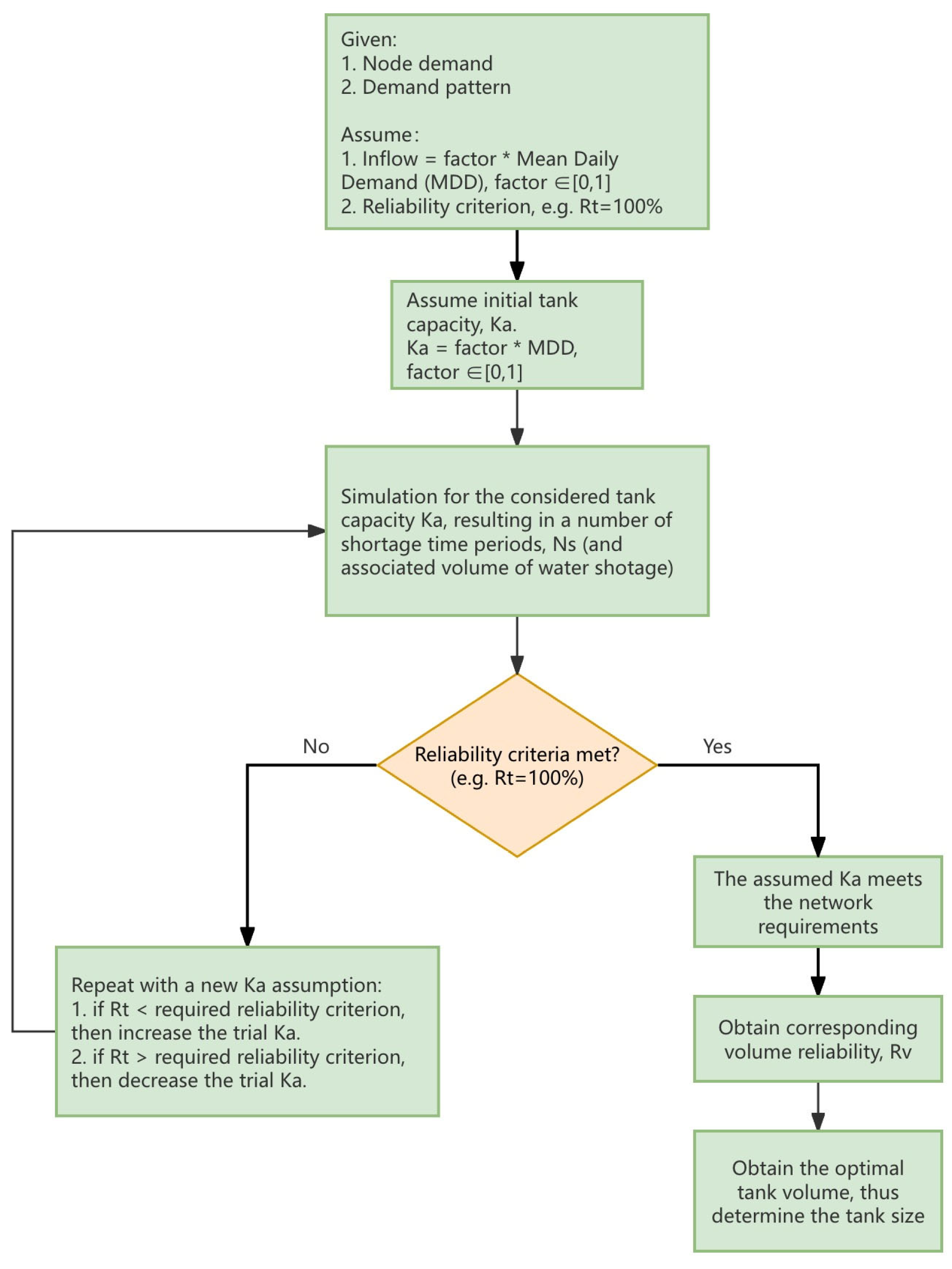
3.1. Behaviour Simulation

Behaviour simulation (BS) is a powerful and practical analytical tool for investigating the main key indicators that describe reservoir performance (such as reliability). It is based on the mass balance equation. As one of the most versatile and widely used methods, BS is able to comprehensively consider the key factors affecting reservoir behaviour.

McMahon and Adeloye [26] and Adeloye et al. [22] also pointed out that BS shows great flexibility and applicability when dealing with problems related to water storage.

This approach can be carried out in the early stages of the design to ensure that the design planning scheme is reasonable. With reference to the calculation of reservoir capacity in existing studies [22,23,26], the formula for calculating the capacity of a water tank can be expressed as

$${\mathrm{S}}_{\mathrm{t}+1}={\mathrm{S}}_{\mathrm{t}}+{\mathrm{Q}}_{\mathrm{t}}-{\mathrm{D}}_{\mathrm{t}}^{\prime }-{\mathrm{B}}_{\mathrm{t}};0\le {\mathrm{S}}_{\mathrm{t}+1}\le {\mathrm{K}}_{\mathrm{a}}$$

(1)

where S_t and S_t+1, respectively, represent the storage state of the tank at the beginning and end of the time period, t; Q_t is the amount of water flowing into the tank during time period t; D_t′ is the amount of water released from the tank during time t; B_t is the backwater generated when the tank is fully filled; and K_a is the capacity of the tank.

Theoretically, the design output of the tank, D_t, should be determined by the total demand of the network while in operation. Depending on the operational scheduling of the system and the availability of water in the system, there is often a discrepancy between the real demand D_t and the released D_t′, and at all times, the following relationship exists:

$${\mathrm{D}}_{\mathrm{t}}\ge {\mathrm{D}}_{\mathrm{t}}^{\prime }$$

(2)

Assuming that the amount of water entering the tank at the beginning of t is known, the total water available in the system during t is

$${\mathrm{W}}_{\mathrm{t}}={\mathrm{S}}_{\mathrm{t}}+{\mathrm{Q}}_{\mathrm{t}}$$

(3)

According to the Standard Operating Policy (SOP) [75], the operation strategy of the water tank is similar to that of the reservoir [22], and the following three scenarios can occur:

• Insufficient water is available to the system, i.e., W_t < D_t;

At this point, the system’s current storage plus the inflow is still insufficient to meet the target release. Therefore, as much water as there is in the system is discharged. The tank is always empty.

$${\mathrm{D}}_{\mathrm{t}}^{\prime }={\mathrm{W}}_{\mathrm{t}}$$

(4)

2.

Sufficient water is available, and the tank is not filled, i.e., D_t ≤ W_t < D_t + K_a.

At this point, the available water in the system is sufficient, and the demands of all users are well met. Some water is stored in the tank, but it does not fill the tank.

$${\mathrm{D}}_{\mathrm{t}}^{\prime }={\mathrm{D}}_{\mathrm{t}}$$

(5)

3.

Sufficient water is available, and the tank is full, i.e., W_t ≥ D_t + K_a.

At this point, the water available in the system is greater than the total demand, and after the tank reaches the storage limit, the excess inflow will produce a backwater phenomenon.

$${\mathrm{D}}_{\mathrm{t}}^{\prime }={\mathrm{W}}_{\mathrm{t}}-{\mathrm{K}}_{\mathrm{a}}$$

(6)

To ensure the water supply’s stability and meet the customers’ basic needs, there should not be any water shortage in the network during the operation period; otherwise, the design solution of the tank is considered to have failed. Based on the water supply performance of the tanks, the BS approach allows for the calculation of two key metrics for determining reliability, namely time-based reliability (R_t) and volume-based reliability (R_v). R_t is the proportion of time that the system can satisfy the demand, whereas R_v is the ratio of the system’s actual volume of water released to the demand. When the tank volume is K_a, the reliability of the system can be expressed by the following formulas:

$${\mathrm{R}}_{\mathrm{t}}=1-{\displaystyle \frac{\sum _{\mathrm{t}=1}^{\mathrm{N}}{\mathrm{f}}_{\mathrm{t}}}{\mathrm{N}}}$$

(7)

$${\mathrm{R}}_{\mathrm{v}}=1-{\displaystyle \frac{\sum _{\mathrm{t}=1}^{\mathrm{N}}{\mathrm{f}}_{\mathrm{t}}\left({\mathrm{D}}_{\mathrm{t}}-{\mathrm{D}}_{\mathrm{t}}^{\prime }\right)}{\sum _{\mathrm{t}=1}^{\mathrm{N}}{\mathrm{D}}_{\mathrm{t}}}}$$

(8)

$${\mathrm{f}}_{\mathrm{t}}=\left\{\begin{array}{c}1,{\mathrm{D}}_{\mathrm{t}}^{\prime }<{\mathrm{D}}_{\mathrm{t}}\\ 0,\mathrm{otherwise}\end{array}\right.$$

(9)

In Equations (7) and (8), N represents the total number of time periods, 24 in our case, and the rest of the symbols have been defined in the previous section.

In the process of tank design, since the K_a requirements may vary for different demand scenarios, to determine the best solution, K_a is usually adjusted through the trial-and-error method until the minimum capacity that can satisfy the given reliability target is found. The process is summarized in Figure 1.

3.2. Vulnerability

Vulnerability can be used as an important index to measure the impact of water shortage in reservoir planning. It is usually determined by the average of the highest water deficits recorded during a simulation of water shortage sequences, thereby assessing the performance of the system under conditions of insufficient water supply [27]. This idea can also be extended to the field of tank design and analysis in urban pipe networks.

In tank design, vulnerability reflects the performance of the tank in response to dynamic demand changes, representing the potential proportion of water shortage under certain conditions. This indicator is critical for assessing the stability and resilience of water supply systems during adverse conditions, making it essential in system design and operation. To comprehensively evaluate the tank’s performance, this study introduced the vulnerability indicator (Vul) to harmonize the deviation between R_t and R_v and further validate the effect of different combinations of inflow and capacity. This approach facilitates the selection of robust, cost-effective designs that improve the reliability and adaptability of water distribution systems under dynamic demand conditions.

First, BS and the corresponding R_v can initially obtain the tank capacity (K_a) that satisfies a particular time-based reliability (R_t). When the value of R_t is not 1, the system is bound to have a water shortage. Let ∆_t represent the proportion of water deficiency at time step t, and it has two situations:

$${∆}_{\mathrm{t}}=\left\{\begin{array}{c}1-\left({\displaystyle \frac{{\mathrm{D}}_{\mathrm{t}}^{\prime }}{\mathrm{D}}}\right)\\ 0; \mathrm{Otherwise}\end{array};\mathrm{f}\mathrm{o}\mathrm{r} {\mathrm{D}}_{\mathrm{t}}^{\prime }<{\mathrm{D}}_{\mathrm{t}}\right.$$

(10)

The vulnerability of the system can be expressed by the following equation:

$$\mathrm{V}\mathrm{u}\mathrm{l}={\displaystyle \frac{\sum _{\mathrm{t}=1}^{\mathrm{N}}\mathrm{m}\mathrm{a}\mathrm{x}{∆}_{\mathrm{t}}}{{\mathrm{f}}_{\mathrm{t}}}}$$

(11)

As discussed in the previous section, D_t and D_t′ denote real demand and actual released demand, respectively. The statistics for the number of failures, f_t, in Equation (11) above are consistent with the method in Equation (9).

Combining the severity and frequency of water supply shortages to calculate vulnerability makes it reflect not only the frequency of water supply shortages but also the depth of their impact. A smaller vulnerability factor indicates that the tank is more adaptable in the face of an insufficient water supply. Especially when faced with scenarios with similar values of R_t and R_v, the vulnerability index can effectively identify and help determine the superior scenario. By making the value of Vul as small as possible, the robustness of the system can be enhanced, thus improving the rationality of the design, making it more consistent with the decision-maker’s comprehensive objectives, and ensuring that the system remains reliable and adaptable under different constraints.

4. Case Study

This work selected two representative water distribution networks for in-depth analysis to verify the application effectiveness of BS in the tank performance simulation. The two subjects are the Sharjah Mughaidir Suburb and the Dubai Silicon Oasis. Their similarities in geographical location, climatic characteristics, and water supply demand, as well as their uniqueness, made them ideal cases for assessing BS methods.

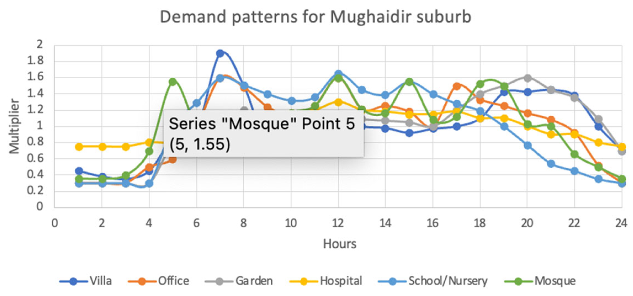
4.1. Case Study #1: Sharjah Mughaidir Suburb

The first example is the Mughaidir Suburb, located in the central city of Sharjah, which consists of six communities and is a typical cluster of communities. The altitude of the study area ranges from 8 m to 25 m above sea level, and the climate is characterized by hot and dry weather throughout the year, especially during the high summer temperatures when the residents’ demand peaks. This long-term high temperature and drought climate further increases the pressure on the water supply system, making the water tank play a vital role in regulating the water supply and guaranteeing the safety of the water supply.

The water distribution network of Sharjah Mughaidir Suburb consists of 83 junctions, 106 pipes, a water pump, and a reservoir. The original design report assumed that water would be supplied directly to the network from the reservoir. To optimize the construction of the system and explore the impact of tank adjustment, this work regarded the reservoir in the original design as a node with inflow, represented by J-36, and introduced a tank, T-1, between this inflow node and the pump for analysis. The adjusted network is shown in Figure 2.

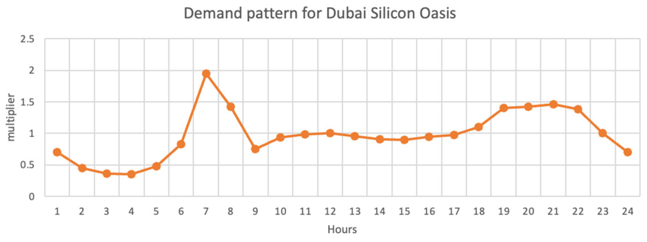
4.2. Case Study #2: Dubai Silicon Oasis

The second example is the Dubai Silicon Oasis, located in the Nadd Hessa community in Dubai, one of Dubai’s key free trade zones. The network consists of 2550 nodes, 2750 pipes, a reservoir, and three pumps operating in parallel. The area contains a variety of building types, such as tower apartments, villa communities, commercial offices, educational institutions, government agencies, hotels, and medical facilities, making the water characteristics of each node complex and varied. Although the current residential population of Dubai Silicon Oasis has not yet reached its expected maximum, the diverse water demand and dynamic water pressure changes in the area provide rich research data for tank design and operation of the water supply system due to its rapid development.

Similarly to the Sharjah Mughaidir Suburb network, the reservoir of the Dubai Silicon Oasis network was considered a node with inflow characteristics, and a tank was set up between the pumps and this node. The schematic of the adjusted network is shown in Figure 3.

4.3. Extended Period Simulation (EPS)

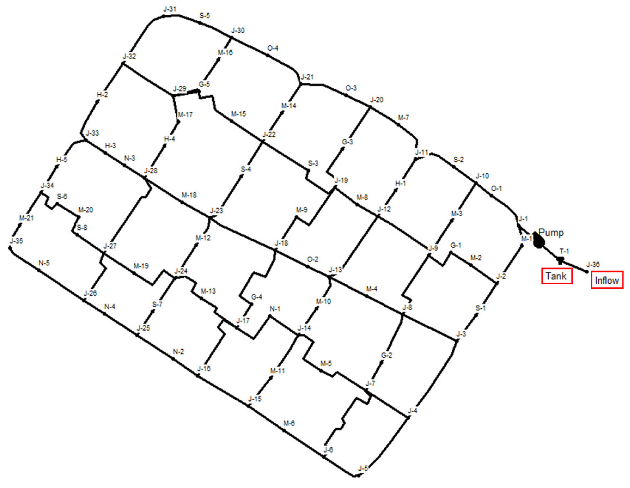
To simulate the operation of the water supply system more realistically in different time periods, water supply network analysis software was used for in-depth modelling analysis. EPANET [80] is a simple and powerful software. This software was created by the United States Environmental Protection Agency (USEPA) and is available as an open source. EPANET allows designers to operate and test their networks and scenarios well in advance of their implementation at the site.

EPANET provides a comprehensive platform for network mapping, data entry, hydraulic simulation and water quality analysis. During simulation, it allows for the monitoring of water flow through pipes, pressure at nodes, tank levels, and changes in concentrations of specific chemicals throughout the network [30,81], as well as analyzing the outcomes in multiple formats such as coloured network maps, tables of data, time-series graphs, and contour charts [30,80,82].

This study discussed the operation of a WDS under different tank capacities and inflow scenarios in 24 h. The dynamic behaviour of the system over time is analyzed using extended period simulation (EPS) with a time step of 1 h. The user demand for each time period varies within a given range, and the demand pattern for the Sharjah Mughaidir Suburb network and Dubai Silicon Oasis network are shown in Figure 4 and Figure 5 below, respectively.

4.4. Modelling

The BS approach was designed to provide an intuitive understanding of changes in K_a and inflow by simulating the system’s dynamic behaviour, helping to identify potential water supply shortfalls or excess situations. On the other hand, the results generated using EPANET could verify the accuracy and validity of the BS method analysis.

Taking the network of Sharjah Mughaidir Suburb as an example, according to building types and demand patterns, the total demand of the system at each time period is counted, as shown in

Table 1. Hourly demand statistics for Sharjah Mughaidir Suburb network.

Time (Hours)	Flow (m3/h)
00:00	391.536
01:00	338.616
02:00	316.728
03:00	416.664
04:00	727.956
05:00	824.688
06:00	1557.792
07:00	1251.468
08:00	702.972
09:00	841.284
10:00	883.080
11:00	979.632
12:00	885.168
13:00	866.484
14:00	831.708
15:00	855.396
16:00	878.508
17:00	956.844
18:00	1192.968
19:00	1180.728
20:00	1182.708
21:00	1119.672
22:00	819.540
23:00	583.344
∑	20,585.484
Average	857.729

.

In practice, the tank does not need to store all the water because there is an inflow in the system, and water is constantly replenished and enters the network. The water level in the tank continuously fluctuates due to the combined effects of inflow rate and K_a. Therefore, to simulate the operation of the network more clearly to determine the appropriate tank size, the specific steps of the experiment are designed as follows:

• Step 1: Network preparation:

The first step of the experiment is to build the water distribution model for the Sharjah Mughaidir Suburb network, set up node demand and demand pattern, extract the total demand of the entire system and calculate Mean Hourly Demand (MHD) and Mean Daily Demand (MDD) to provide the basis for inflow and K_a grading.

• Step 2: Grading of inflow and K_a:
  For a clearer comparison of the design options, the inflow and K_a are graded on a 10% gradient. The specific grading is as follows:
  • Inflow is defined as
  $$\mathrm{I}\mathrm{n}\mathrm{f}\mathrm{l}\mathrm{o}\mathrm{w}=\mathrm{f}\mathrm{a}\mathrm{c}\mathrm{t}\mathrm{o}\mathrm{r} 1\times \mathrm{M}\mathrm{H}\mathrm{D}$$

  (12)
  • Tank capacity (K_a) is defined as
  $${\mathrm{K}}_{\mathrm{a}}=\mathrm{f}\mathrm{a}\mathrm{c}\mathrm{t}\mathrm{o}\mathrm{r} 2\times \mathrm{M}\mathrm{D}\mathrm{D}$$

  (13)

Factors 1 and 2 both range from 0.1 to 1.0 in 0.1 increments. This gives a total of 100 different combinations of inflow and K_a scenarios.

Table 2. Inflow with different factors for Sharjah Mughaidir Suburb network.

Inflow/MHD	Inflow (m3/h)
0.1	85.774
0.2	171.547
0.3	257.317
0.4	343.091
0.5	428.864
0.6	514.638
0.7	600.412
0.8	686.182
0.9	771.955
1	857.729

and

Table 3. Tank volume with different factors for Sharjah Mughaidir Suburb network.

Ka/MDD	Ka (m3)
0.1	2058.548
0.2	4117.097
0.3	6175.645
0.4	8234.194
0.5	10,292.742
0.6	12,351.29
0.7	14,409.839
0.8	16,468.387
0.9	18,526.936
1	20,585.484

summarize the corresponding inflow and tank capacities for each factor in the network.

• Step 3: Implementation of BS:

It is assumed that the tank is full at the beginning of the day and set a fixed inflow; for example, inflow = 0.1 * MHD. Then, the operating results of the system for each hour are sequentially calculated, and K_a is gradually increased from 0.1 MDD to 1.0 MDD. The corresponding number of failures and water deficiency within 24 h periods are calculated and counted. The inflow is adjusted and this step is repeated until all scenarios are completed.

• Step 4: Reliability calculations:

Based on the results obtained in step 3, the R_t and R_v of each scheme are further calculated to quantify their performance against unstable demands and evaluate the water supply safety and stability of the tank design.

• Step 5: Simulation in EPANET:

To ensure the accuracy and applicability of the BS, further validation is carried out in EPANET. Assuming that the tank is cylindrical and has a height of 5 m, the diameter of the tank is obtained based on the calculated K_a in Table 3. The calculation formula is

$$\mathrm{D}=\sqrt{{\displaystyle \frac{4\times {\mathrm{K}}_{\mathrm{a}}}{\mathsf{\pi }\times \mathrm{h}}}}$$

(14)

The tank size and inflow are entered into EPANET for EPS analysis to obtain detailed operational reports for each combination scenario. The corresponding reliability of each scheme, i.e., R_{t, EPANET}, is calculated.

• Step 6: Comparison and analysis of results

The results of BS and EPANET are compared to verify the accuracy and consistency of the analysis. Combined with the R_t and R_v simulation results of each scenario, the system stability is weighed against other key decision factors to provide a basis and guidance for the development of scientific and reasonable scenarios.

Following the same procedures, the Dubai Silicon Oasis network data are systematically processed and calculated. The values of relevant parameters are shown in

Table 4. Hourly demand statistics for the Dubai Silicon Oasis network.

Time (Hours)	Flow (m3/h)
00:00	1211.328
01:00	778.680
02:00	622.944
03:00	605.664
04:00	830.628
05:00	1436.292
06:00	3374.460
07:00	2457.324
08:00	1297.836
09:00	1626.696
10:00	1695.924
11:00	1730.484
12:00	1661.256
13:00	1574.748
14:00	1557.468
15:00	1643.976
16:00	1678.536
17:00	1903.500
18:00	2422.656
19:00	2457.324
20:00	2526.552
21:00	2388.096
22:00	1730.484
23:00	1211.328
∑	40,424.184
Average	1684.341

,

Table 5. Inflow with different factors for Dubai Silicon Oasis network.

Inflow/MHD	Inflow (m3/h)
0.1	168.433
0.2	336.870
0.3	505.303
0.4	673.736
0.5	842.170
0.6	1010.606
0.7	1179.040
0.8	1347.473
0.9	1515.906
1	1684.343

and

Table 6. Tank volume with different factors for Dubai Silicon Oasis network.

Ka/MDD	Ka (m3)
0.1	4042.418
0.2	8084.837
0.3	12,127.255
0.4	16,169.674
0.5	20,212.092
0.6	24,254.510
0.7	28,296.929
0.8	32,339.347
0.9	36,381.766
1	40,424.184

.

5. Results and Discussion

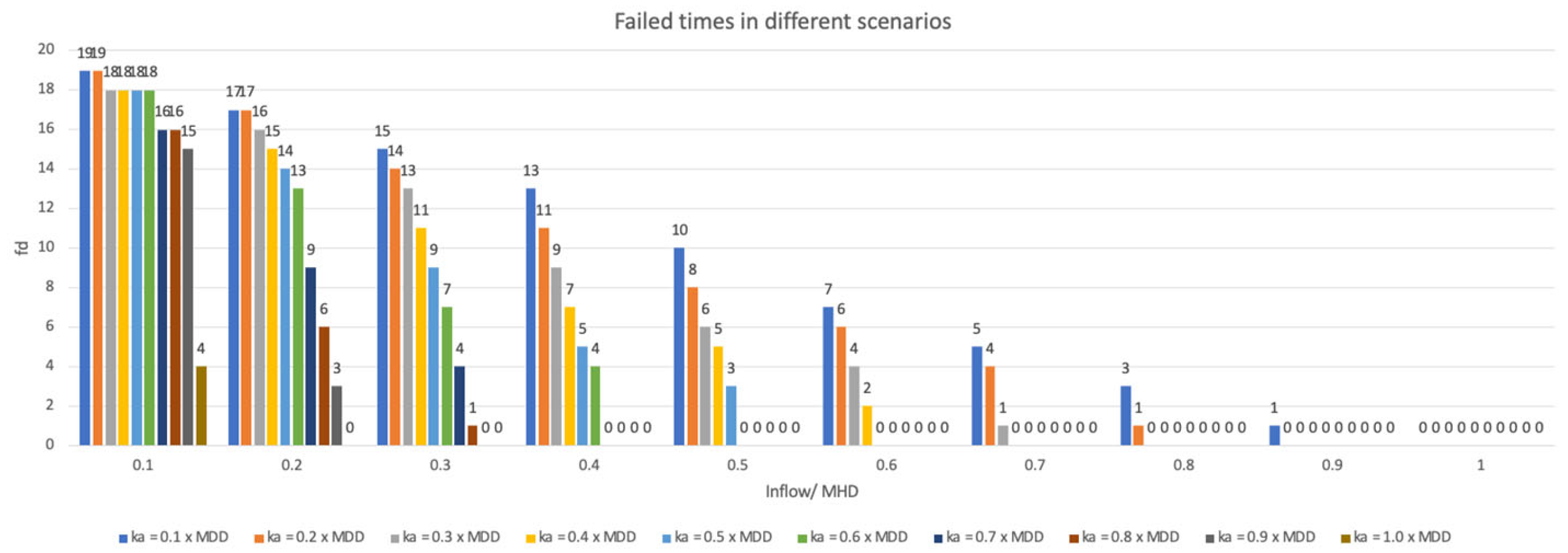
5.1. Network Failure

A comprehensive analysis of 100 combination scenarios of inflow and capacity (K_a) for the two networks was performed using Excel. The results showed that the two networks exhibited a similar trend under the analysis of the BS method, indicating that the changes in inflow and K_a have a direct and significant impact on the success of the water supply. To compare the data more visually, Figure 6 and Figure 7 present the statistics of the two networks in the form of bar charts.

When the inflow is low (e.g., 0.1–0.3 MHD), the number of water supply failures is generally high regardless of the K_a, and the maximum number of water shortages can reach 19 times in a single day. This is because the system is unable to store sufficient water during off-peak hours to cope with the water demand during peak hours. Even if the tanks have a relatively large capacity, there is a lack of sufficient water to fill them, resulting in a limitation of the regulating effect of the tanks. As the inflow increases, especially when the inflow reaches 0.4 MHD and above, the number of system failures begins to decline, and if the system is configured with a medium-capacity tank, the number of failures is basically controlled within 10 times. A higher inflow volume can quickly replenish water for the network, which helps to improve the success rate of the tank water supply, thereby improving the reliability of the system.

On the other hand, larger-capacity tanks (e.g., 0.5 MDD and above) significantly reduced the number of failures. Even with the smallest inflow, the Sharjah Mughaidir Suburb network only has 10 failures in 24 h, compared to 9 failures for the Dubai Silicon Oasis network. When the inflow is stabilized at 0.6 MHD, for either network in the case study, only a water tank with a capacity of 0.5 MDD is required to achieve a 100% success rate.

Larger tanks are better able to cope with peak demand and short-term fluctuations in water supply. However, the high success rate is accompanied by a significant increase in tank size. This is not only economically problematic but also brings huge adjustments in terms of land use, construction costs, operation and maintenance, and water quality. Such large tanks run counter to the goal of “sustainable design”. In addition, excessive tank capacity leads to slow water renewal in the WDS, which in turn can lead to poor mixing and water ageing phenomena, affecting water quality and safety [3,5,83]. Excessive retention time reduces the concentration of disinfectants (e.g., chlorine) and thus weakens the inhibition of microbial growth [55]. This leads to bacterial growth and can trigger temperature or chemical stratification within the tank, leading to uneven water quality. Therefore, although pursuing a 100% success rate is theoretically feasible, it is often necessary to design the tank through reliability evaluation to balance performance with practical requirements.

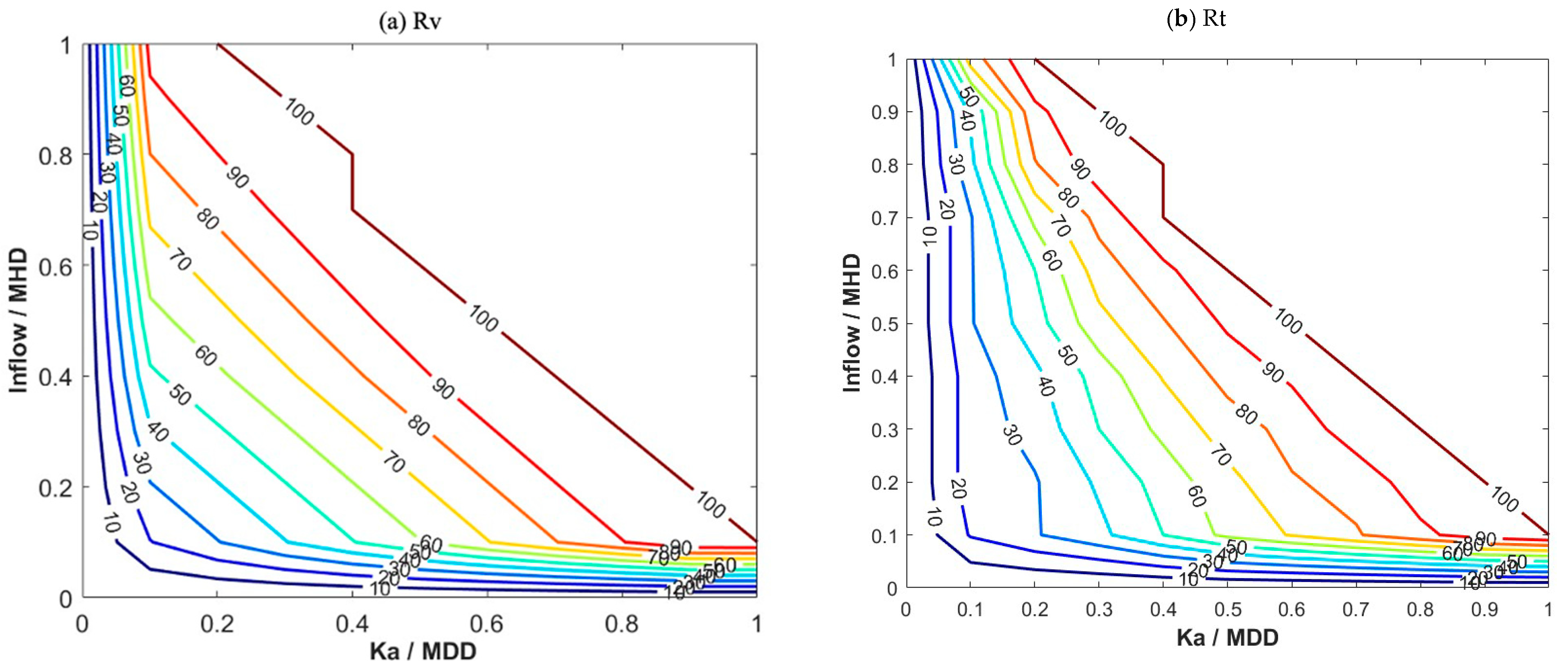
5.2. System Reliability

The network’s time-based reliability (R_t) can be calculated according to the number of water supply failures in 24 h. At the same time, the network’s desired demand and release demand provide a basis for calculating volume-based reliability (R_v). As they are defined, R_t and R_v evaluate the performance of a water distribution network from different perspectives. The former examines the proportion of the time the system can meet the demand for water supply in a given period, focusing on the temporal dimension of water supply, and is a purely temporal success assessment. On the other hand, the latter focuses on the adequacy of the water supply and evaluates the proportion of actual water supply to the demanded water supply in a given time period. It is an assessment that focuses more on the adequacy and satisfaction of the volume of water supplied rather than just considering whether the water supply was successful.

Based on the reliability results obtained using the BS method, the capacity–inflow–reliability curves can be drawn, as shown in Figure 8a,b and Figure 9a,b. The contour lines in the figures show the changing patterns of Sharjah Mughaidir Suburb and Dubai Silicon Oasis networks at different reliability levels (0% to 100%), respectively.

At small tank capacities (e.g., K_a = 0.1 MDD or 0.2 MDD), R_v improves significantly faster than R_t as inflow increases. This indicates that in the case of small tank volume, increasing the inflow has a greater effect on improving the overall performance of the WDS. From the comparison of R_t and R_v, it can also be found that R_v is greater than or equal to R_t in both Sharjah Mughaidir Suburb and Dubai Silicon Oasis networks. For example, in the Dubai Silicon Oasis network, when Inflow is 0.5 MHD and K_a is 0.4 MDD, the values of R_t and R_v are 0.792 and 0.875, respectively. The reason for the difference is that the determination criteria of R_t are stricter. For R_v, as long as the total water supply of the system can meet the requirements, even if the water supply is insufficient in individual periods, it will not be regarded as a failure. With a low inflow, the tank can accumulate enough water in certain periods to cope with subsequent high-demand phases. R_t, on the other hand, requires that the demand be met every hour, and even if the water supply exceeds the demand in a certain period, it does not compensate for the failure in a previous period. Therefore, this “compensation effect” is ineffective, which explains why R_v tends to be greater than R_t.

In addition, changes in the spacing of neighbouring contour lines directly reflect the system’s sensitivity and responsiveness to demand fluctuations. At both ends of the contour lines, i.e., the region where inflow/MHD and K_a/MDD are close to 1, the neighbouring contour lines are closer together. This suggests that the reliability can quickly jump to another level if the design parameters change slightly. In contrast, in the middle region of the figure, the neighbouring contour lines are farther apart. This means the design parameters are free to vary within a certain range without significantly changing the reliability level of the system. This “tolerance zone” shows more design flexibility. The configuration within this zone can be stabilized within the target reliability range even when the system undergoes operational deviations. For example, in the Sharjah Mughaidir Suburb network, if K_a is 0.5 MDD and the inflow is 0.6 MHD, the system’s R_v can reach 100%; even though the inflow drops to 0.5 MHD, the system reliability can still be maintained at approximately 95%, which is much more fault tolerant and thus more applicable to deal with the uncertainty in future demands.

For any network, the core of reliability lies in the reasonable matching of capacity and inflow. Once the reliability target is determined, the capacity–inflow–reliability curve based on the BS method will help the decision-maker quickly identify a suitable combination of capacity and inflow. This serves as the basis for flexible planning of resource allocation and adjustment of design options, ensuring that the system can meet the target demand. Therefore, these figures not only reveal the relationship between reliability and design parameters but generate a range of alternatives that can be selected by designers or operators through the reliability contour lines, providing strong support for achieving a balance between reliability and other objectives.

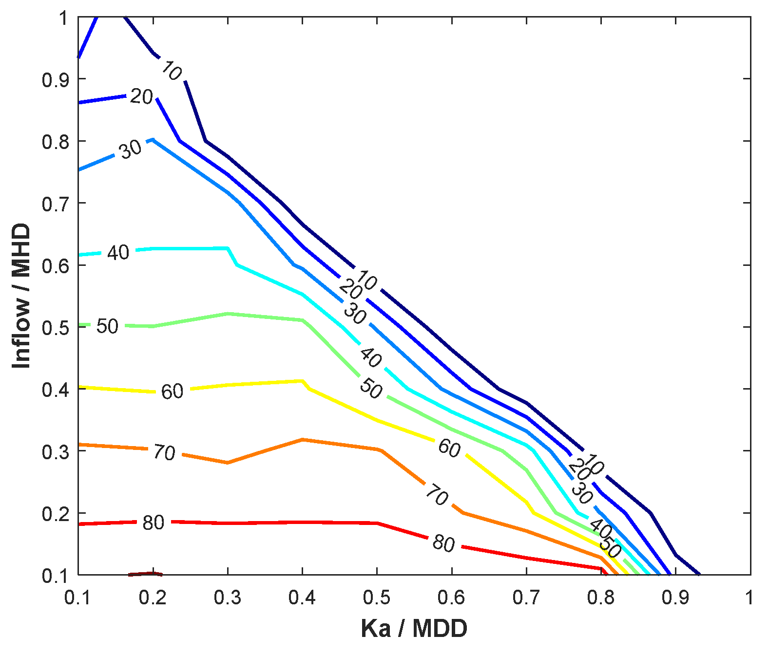
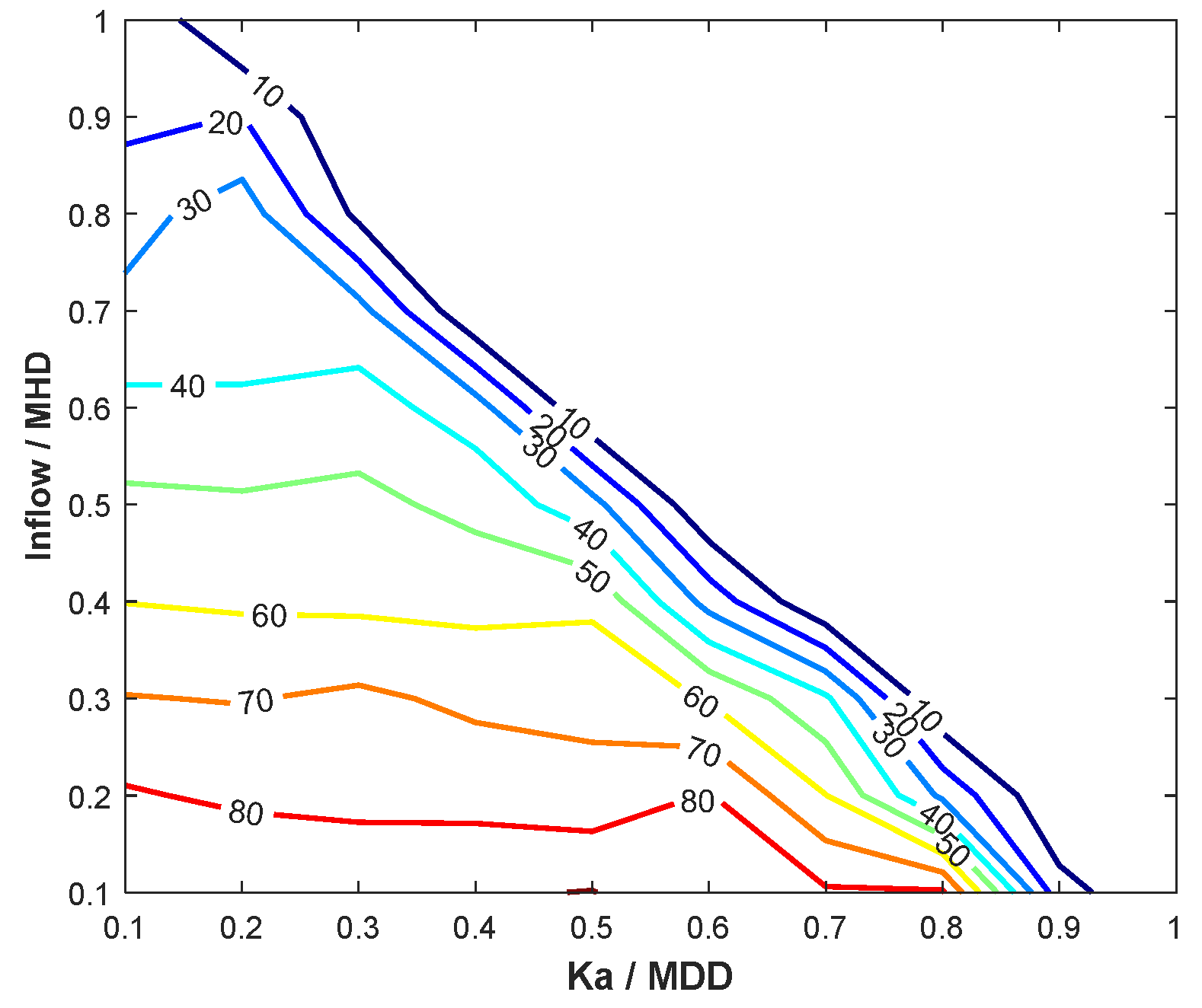
5.3. Vulnerability Assessment

The concept of vulnerability represents the performance of a system under extreme conditions, such as high demand or low water supply. WDS vulnerability evaluation can be used to analyze the system’s adaptability and coping ability under insufficient water supply. This is one of the key indicators in determining the design effectiveness of the system. The contour lines in Figure 10 and Figure 11 show the corresponding vulnerability of the Sharjah Mughaidir Suburb network and Dubai Silicon Oasis network under different inflow and tank capacity (K_a) combinations.

At lower inflows (e.g., inflow = 0.1 MHD), the vulnerability values are consistently higher, indicating a more severe water supply shortage problem. For example, when the tank volume of the Sharjah Mughaidir Suburb network is 0.1 MDD, the vulnerability is 0.894, and when the capacity is increased to 0.5 MDD, the vulnerability only slightly decreases to 0.855. The system’s vulnerability gradually decreases when the inflow is raised to 0.4 MHD. For example, when the K_a is 0.1 MDD, the vulnerability is 0.603. When the K_a is increased to 0.5 MDD, the vulnerability further decreases to 0.491. This suggests that under the condition of low inflow, the increase in K_a has a limited effect on the vulnerability improvement, and the insufficiency of inflow itself mainly limits the system’s water supply capacity. However, under medium inflow, an appropriate increase in K_a has a better effect on coping with moderate water supply–demand fluctuations and can significantly reduce the system’s vulnerability.

Even among scenarios with similar or identical reliability, vulnerability may show significant differences. For example, in the Dubai Silicon Oasis network, the combinations of inflow and K_a at 0.4 MHD and 0.4 MDD, as well as 0.3 MHD and 0.5 MDD, although the R_v are close (0.783 and 0.788, respectively), the corresponding vulnerabilities are significantly different, with values of 0.570 and 0.668, respectively. Similarly, for the combinations of inflow and K_a of 0.9 MHD and 0.2 MDD, 0.6 MHD and 0.4 MDD, and 0.1 MHD and 0.8 MDD, the vulnerability variations are significant at 0.203, 0.347, and 0.812, respectively, even though they have equal R_t values (all 0.875).

Overall, with the increase in K_a, the vulnerability gradually decreases, indicating that the higher the K_a, the more stable the system. Contour lines with higher vulnerability are flatter, such as 80% or 90%. At this time, the system itself is already in a relatively poor state and is very prone to water supply deficiencies. Even increasing the capacity or inflow will not significantly improve the system’s ability to supply water, so the contour lines are sparsely distributed and flat. In practice, such options should be avoided as much as possible. On the contrary, low-vulnerability areas are extremely sensitive to design parameters, with dense and steep contours. When the vulnerability is close to 10% or 20%, the design of the system is already close to “optimal”, and any small change may quickly deplete the water supply margin, leading to a rapid deterioration of the vulnerability.

In the design of WDSs, it is difficult for a single reliability index to fully reflect the real stability of the system, while the vulnerability index can provide a more detailed analysis. The combination of reliability and vulnerability contour lines enables the accurate regulation of parameters and the prediction of potential fluctuations to ensure that the system has a certain degree of immunity and adaptability while meeting the high-reliability requirements.

5.4. EPANET Modelling Result Comparison

This study used EPANET to conduct hydraulic simulation for all scenarios and obtain detailed running reports under various combination conditions. These reports provided comprehensive information on the operation status, failure time, and number of failures of each scenario under different conditions. The operation reports for both networks show that the time of the first occurrence of a water supply failure in the system is gradually delayed as the inflow increases, and this trend also applies to the condition of increasing tank volume, i.e., the water supply guarantee time of the system is extended accordingly as the K_a increases.

Subsequently, based on the number of failures and overall performance of each scenario in the simulation records, the two networks’ time-based reliability (R_t) based on the operation results in EPANET is calculated and summarized separately and the corresponding contour lines as shown in Figure 12 and Figure 13.

Figure 8b, Figure 9b, Figure 12 and Figure 13 show the variation in time-based reliability (R_t) with tank capacity (K_a/MDD) and inflow (inflow/MHD) for the same distribution network analyzed by the BS method and EPANET software (Version 2.2), respectively. The reliability contour lines generated based on the BS method are steeper in the low-capacity and low-inflow regions, suggesting that the BS method is more effective in capturing the subtle variations in low-capacity and low-inflow conditions, allowing for a more accurate selection of design parameters. The results of the two methods in the high-reliability region are similar, indicating a consistent assessment. With the increase in K_a, the curve performance of the two methods gradually draws closer to each other. When the tank volume reaches 0.7 MDD or larger, the curves of the two methods almost coincide, and the R_t tends to 100% regardless of the inflow level, indicating that at this point, the tank’s storage capacity has exceeded the system demand and is overdesigned.

The results obtained using EPANET are more “optimistic” for small tanks. This optimism is mainly manifested in fewer failures and higher reliability. However, it also means that EPANET may overestimate the reliability of the WDS in some cases, especially in scenarios with high flow fluctuations or high demand periods. In contrast, using the BS approach in designing the tank and analyzing the operation of the WDS makes it easier to capture the situation of insufficient water supply, thus providing a more reliable design reference. The BS method is more suitable for evaluating the minimum acceptable performance of a system because it does not use hydraulic delay or other mechanisms to mask the system’s water supply.

5.5. Comparison with the Literature

In conjunction with similar studies in the references, this study shares some methodological similarities with the study by Adeloye et al. [22], both of which use BS as the core analytical method for evaluating the reliability index of the system. This demonstrates the wide applicability of the BS method in evaluating the performance of water resource systems, enabling the construction of various operational scenarios for reservoir planning and urban water tank design. By doing so, it helps decision-makers expand the horizon of their analysis and provides them with more flexible and scientifically grounded choices.

The difference in research objects determines the focus of the research. Reservoir design focuses on macroscopic hydrological challenges such as runoff fluctuations and long-term storage demands, whereas urban tank design focuses more on stabilization of water supply, pressure control, spatial utilization, and cost optimization under dynamic water supply demand. Nevertheless, both studies systematically evaluated the reliability indicators (time-based and volume-based) and enabled the results to provide strong support for design and operation. For example, the study by Adeloye et al. [22] stated that reliability in reservoir planning is strongly influenced by runoff variability (CV). Through graphs, the study clearly demonstrated the relationship between demand, capacity and reliability under different CV conditions. It introduced water shortage thresholds to coordinate the differences between R_t and R_v, providing a scientific basis for the development of reservoirs for water storage functions.

This study further extends the application of the behaviour simulation (BS) method. By generating BS-derived capacity–inflow–reliability curves and combining them with vulnerability indicators, tank configurations with the same or similar reliability are analyzed in detail, enabling engineers to visually assess the feasibility and performance of various scenarios and providing decision-makers with a multi-dimensional selection space. This analysis not only helps designers and managers to systematically compare the advantages and disadvantages of various options but also expands the research perspectives on the optimal design of closed storage tanks, providing a more flexible and scientific decision-making basis for the optimal configuration of water systems. These research results deepen the theoretical value and practical application potential of the BS method in various water management scenarios and provide valuable references for future research and practical engineering applications.

6. Conclusions and Future Work

This study focuses on the design of tanks in urban WDSs, aiming to explore the reliability and stability of the water distribution network under different combinations of tank volume and inflow to support better tank configuration decisions in practical projects. During this study, a detailed simulation of the water distribution network of two typical communities located in the UAE, the Sharjah Mughaidir Suburb community and the Dubai Silicon Oasis community, was carried out by introducing the BS method. For the water supply performance under different conditions, this study systematically examines the impact of water tank design on the water supply success and time and capacity reliability of the distribution network. BS’s applicability and analyzed differences in water tank design were also verified in conjunction with EPANET software, which provides a targeted reference for future water distribution network design.

The experimental results show that tank capacity (K_a) and inflow are two key factors affecting the reliability of the water distribution network. To intuitively show the impact of changes in design parameters on system reliability, the capacity–inflow–reliability curves, which are drawn based on the BS analysis method, clearly reflect the reliability changes in the network under different configurations. These curves provide designers with a convenient tool that can help decision-makers quickly determine the appropriate configuration to meet the target reliability, helping them to weigh the relationship between tank capacity, matching supply and demand, and system reliability under different constraints.

In the process of analysis, the differences and reasons for time-based reliability (R_t) and volume-based reliability (R_v) in reliability evaluation are also investigated, which provides an important reference for decision-makers in data analysis so that they can make more reasonable choices in decision-making. To further observe the responsiveness of the system, the vulnerability index is used to analyze the water supply performance of the network under different tank configurations. The results show that lower vulnerability values imply that the system is able to maintain higher stability and reflect greater adaptability when the water supply is insufficient.

The relevant data obtained from the WDS in Sharjah and Dubai showed that the BS method is similar to the results of the EPANET simulation, verifying the accuracy and applicability of the BS method in modelling the performance of water tanks. Moreover, BS has stricter criteria and hence is able to underline the differences among different scenarios with more precision. This not only provides a more intuitive reference for tank design but also effectively supports decision-makers in developing more adaptive management strategies in complex water supply environments, making it a quicker and easier tool for engineers.

Although the BS method had been applied to the planning and assessment of open waters in the past study by Adeloye et al. [22], this study introduced the BS method into the design of tanks for WDSs and successfully verified its applicability to the analysis of urban water distribution networks. The study explores the tank’s operation in various configurations through simulations in different scenarios to generate a range of alternatives that the operator can select. This provides valuable experience for practical engineering design and management of WDSs. It also has potential application value in increasing management efficiency and safety for WDS improvement.

The cases selected for this study are all located in a tropical desert climate region, which is dry and hot all year round and has low seasonal fluctuations in water demand. Therefore, although this study validates the effectiveness of the BS method in tank design, the specific conclusions of the analyses need to be adjusted accordingly to the climatic characteristics and demand fluctuations of the regions where they are located. However, in regions with variable climate, abundant precipitation, or strong seasonal fluctuations in water demand, the generated BS-based iso-reliability plots can still provide a valuable reference for tank design. In addition, this study only considered fixed demand patterns in the analysis and failed to cover all cases of abnormal demand fluctuations and unexpected events. Future research can incorporate geographical characteristics and operational uncertainty factors to comprehensively evaluate the system’s stability under various extreme conditions to further improve the scientific and applicability of options for tank design.

References

1. van Zyl, J.E.; Piller, O.; le Gat, Y. Sizing Municipal Storage Tanks Based on Reliability Criteria. J. Water Resour. Plan. Manag. 2008, 134, 548–555. [Google Scholar] [CrossRef]
2. Gupta, A.D.; Bokde, N.; Marathe, D.; Kulat, K. Optimization techniques for leakage management in urban water distribution networks. Water Sci. Technol. Water Supply 2017, 17, 1638–1652. [Google Scholar] [CrossRef]
3. Zhang, J. Approaches for estimating mixing time in a water storage tank. Water Sci. Technol. Water Supply 2022, 22, 3769–3783. [Google Scholar] [CrossRef]
4. Batchabani, E.; Fuamba, M. Optimal Tank Design in Water Distribution Networks: Review of Literature and Perspectives. J. Water Resour. Plan. Manag. 2014, 140, 136–145. [Google Scholar] [CrossRef]
5. Abrha, B.; Ostfeld, A. Analytical Solutions to Conservative and Non-Conservative Water Quality Constituents in Water Distribution System Storage Tanks. Water 2021, 13, 3502. [Google Scholar] [CrossRef]
6. Alperovits, E.; Shamir, U. Design of optimal water distribution systems. Water Resour. Res. 1977, 13, 885–900. [Google Scholar] [CrossRef]
7. Sherali, H.D.; Totlani, R.; Loganathan, G.V. Enhanced lower bounds for the global optimization of water distribution networks. Water Resour. Res. 1998, 34, 1831–1841. [Google Scholar] [CrossRef]
8. Puleo, V.; Morley, M.; Freni, G.; Savić, D. Multi-stage linear programming optimization for pump scheduling. Procedia Eng. 2014, 70, 1378–1385. [Google Scholar] [CrossRef]
9. Fujiwara, O.; Khang, D.B. A two-phase decomposition method for optimal design of looped water distribution networks. Water Resour. Res. 1990, 26, 539–549. [Google Scholar] [CrossRef]
10. Pandey, S.; Singh, R.P.; Mahar, P.S. Optimal Pipe Sizing and Operation of Multistage Centrifugal Pumps for Water Supply. J. Pipeline Syst. 2020, 11, 4020007. [Google Scholar] [CrossRef]
11. Maskit, M.; Ostfeld, A. Multi-Objective Operation-Leakage Optimization and Calibration of Water Distribution Systems. Water 2021, 13, 1606. [Google Scholar] [CrossRef]
12. Murphy, L.J.; Dandy, G.C.; Simpson, A.R. (Eds.) Optimum design and operation of pumped water distribution systems. In Proceedings of the National Conference Publication-Institution of Engineers Australia NCP, Melbourne, Australia, 13–16 April 1994; p. 149. [Google Scholar]
13. Prasad, T.D. Design of Pumped Water Distribution Networks with Storage. J. Water Resour. Plan. Manag. 2010, 136, 129–132. [Google Scholar] [CrossRef]
14. Luna, T.; Ribau, J.; Figueiredo, D.; Alves, R. Improving energy efficiency in water supply systems with pump scheduling optimization. J. Clean. Prod. 2019, 213, 342–356. [Google Scholar] [CrossRef]
15. Zhao, Y.; Zhang, P.; Pu, Y.; Lei, H.; Zheng, X. Unit Operation Combination and Flow Distribution Scheme of Water Pump Station System Based on Genetic Algorithm. Appl. Sci. 2023, 13, 11869. [Google Scholar] [CrossRef]
16. Ostfeld, A.; Tubaltzev, A. Ant Colony Optimization for Least-Cost Design and Operation of Pumping Water Distribution Systems. J. Water Resour. Plan. Manag. 2008, 134, 107–118. [Google Scholar] [CrossRef]
17. Hajibandeh, E.; Nazif, S. Pressure Zoning Approach for Leak Detection in Water Distribution Systems Based on a Multi Objective Ant Colony Optimization. Water Resour. Manag. 2018, 32, 2287–2300. [Google Scholar] [CrossRef]
18. Ahmadi, M.H.; Mansoori, B.; Aghamajidi, R. Optimization of chlorine consumption in water distribution networks by using the new ant colony optimization (ACOR) algorithm. Int. J. Environ. Sci. Technol. 2024, 22, 3199–3212. [Google Scholar] [CrossRef]
19. Wegley, C.; Eusuff, M.; Lansey, K. Determining pump operations using particle swarm optimization. In Building Partnerships; American Society of Civil Engineers: Reston, VA, USA, 2000; pp. 1–6. [Google Scholar]
20. Sheikholeslami, R.; Talatahari, S. Developed Swarm Optimizer: A New Method for Sizing Optimization of Water Distribution Systems. J. Comput. Civ. Eng. 2016, 30, 04016005. [Google Scholar] [CrossRef]
21. Jafari-Asl, J.; Sami Kashkooli, B.; Bahrami, M. Using particle swarm optimization algorithm to optimally locating and controlling of pressure reducing valves for leakage minimization in water distribution systems. Sustain. Water Resour. Manag. 2020, 6, 64. [Google Scholar] [CrossRef]
22. Adeloye, A.J.; Soundharajan, B.-S.; Mohammed, S. Harmonisation of Reliability Performance Indices for Planning and Operational Evaluation of Water Supply Reservoirs. Water Resour. Manag. 2017, 31, 1013–1029. [Google Scholar] [CrossRef]
23. Adeloye, A.J.; Dau, Q.V. Hedging as an adaptive measure for climate change induced water shortage at the Pong reservoir in the Indus Basin Beas River, India. Sci. Total Environ. 2019, 687, 554–566. [Google Scholar] [CrossRef] [PubMed]
24. Anirbid, S.; Kriti, Y.; Kamakshi, R.; Namrata, B.; Hemangi, O. Application of machine learning and artificial intelligence in oil and gas industry. Pet. Res. 2021, 6, 379–391. [Google Scholar]
25. Wagner, J.M.; Shamir, U.; Marks, D.H. Water Distribution Reliability: Simulation Methods. J. Water Resour. Plan. Manag. 1988, 114, 276–294. [Google Scholar] [CrossRef]
26. McMahon, T.A.; Adeloye, A.J. Water Resources Yield; McMahon, T.A., Adeloye, A.J., Eds.; Water Resources Publication: Littleton, CO, USA, 2005. [Google Scholar]
27. Adeloye, A. Hydrological sizing of water supply reservoirs. In Encyclopedia of Lakes and Reservoirs; Bengtsson, L., Herschy, R.W., Fairbridge, R.W., Eds.; Springer: Berlin/Heidelberg, Germany, 2012; pp. 346–355. [Google Scholar]
28. Perelman, L.; Ostfeld, A. Topological clustering for water distribution systems analysis. Environ. Model. Softw. Environ. Data News 2011, 26, 969–972. [Google Scholar] [CrossRef]
29. Steinebach, G.; Rosen, R.; Sohr, A.; Morsi, A.; Oberlack, M.; Klamroth, K.; Leugering, G.; Lang, J.; Martin, A.; Ostrowski, M. Modeling and Numerical Simulation of Pipe Flow Problems in Water Supply Systems. In Mathematical Optimization of Water Networks; Birkhäuser: Basel, Switzerland, 2012; pp. 3–15. [Google Scholar] [CrossRef]
30. Kumar, A.; Kumar, K.; Bharanidharan, B.; Matial, N.; Dey, E.; Singh, M.; Thakur, V.; Sharma, S.; Malhotra, N. Design of water distribution system using EPANET. Int. J. Adv. Res. 2015, 3, 789–812. [Google Scholar]
31. Hooda, N.; Damani, O. JalTantra: A System for the Design and Optimization of Rural Piped Water Networks. INFORMS J. Appl. Anal. 2019, 49, 447–458. [Google Scholar] [CrossRef]
32. Marlim, M.S.; Jeong, G.; Kang, D. Identification of critical pipes using a criticality index in water distribution networks. Appl. Sci. 2019, 9, 4052. [Google Scholar] [CrossRef]
33. Albarakati, A.; Tassaddiq, A.; Srivastava, R. Assessment of the Water Distribution Networks in the Kingdom of Saudi Arabia: A Mathematical Model. Axioms 2023, 12, 1055. [Google Scholar] [CrossRef]
34. Janzen, J.G.; Freire, I.L. Evaluation of Disinfection Cost for Different Flow Regimes in Water Storage Tanks. J. Water Resour. Plan. Manag. 2021, 147, 06021004. [Google Scholar] [CrossRef]
35. Pinheiro, A.; Monteiro, L.; Carneiro, J.; do Céu Almeida, M.; Covas, D. Water Mixing and Renewal in Circular Cross-Section Storage Tanks as Influenced by Configuration and Operational Conditions. J. Hydraul. Eng. 2021, 147, 04021050. [Google Scholar] [CrossRef]
36. Ortega-Ballesteros, A.; Muñoz-Rodríguez, D.; Perea-Moreno, A.-J. Advances in Leakage Control and Energy Consumption Optimization in Drinking Water Distribution Networks. Energies 2022, 15, 5484. [Google Scholar] [CrossRef]
37. Mala-Jetmarova, H.; Sultanova, N.; Savic, D. Lost in optimisation of water distribution systems? A literature review of system operation. Environ. Model. Softw. 2017, 93, 209–254. [Google Scholar] [CrossRef]
38. Muwini, R.; Mulayi, S.A.M. Simulation-optimization model for design of water distribution system using ant based algorithms. J. Eng. Res. (Print) 2018, 15, 42–60. [Google Scholar] [CrossRef]
39. Sulianto; Setiono, E.; Yasa, I.W. Optimization model the pipe diameter in the drinking water distribution network using multi-objective genetic algorithm. J. Water Land Dev. 2021, 48, 55–64. [Google Scholar] [CrossRef]
40. Sulianto, S.; Darmawan, A.A.; Andardi, F.R.; Sumadi, F.D.S.; Rahmandhika, A.; Setyawan, N.; Utama, D.M.; Rahim, R. Optimization model of pipe diameter in drinking water distribution network using a combination of the Newton Raphson method and the Codeq algorithm. In AIP Conference Proceedings; AIP Publishing: Melville, NY, USA, 2024; Volume 2927. [Google Scholar] [CrossRef]
41. Carpitella, S.; Brentan, B.; Montalvo, I.; Izquierdo, J.; Certa, A. Multi-criteria analysis applied to multi-objective optimal pump scheduling in water systems. Water Sci. Technol. Water Supply 2019, 19, 2338–2346. [Google Scholar] [CrossRef]
42. Martin-Candilejo, A.; Santillán, D.; Garrote, L. Pump Efficiency Analysis for Proper Energy Assessment in Optimization of Water Supply Systems. Water 2020, 12, 132. [Google Scholar] [CrossRef]
43. Hajgató, G.; Paál, G.; Gyires-Tóth, B. Deep Reinforcement Learning for Real-Time Optimization of Pumps in Water Distribution Systems. J. Water Resour. Plan. Manag. 2020, 146, 04020079. [Google Scholar] [CrossRef]
44. Shao, Y.; Zhou, X.; Yu, T.; Zhang, T.; Chu, S. Pump scheduling optimization in water distribution system based on mixed integer linear programming. Eur. J. Oper. Res. 2024, 313, 1140–1151. [Google Scholar] [CrossRef]
45. Farmani, R.; Savic, D.; Walters, G. The Simultaneous Multi-Objective Optimization of Anytown Pipe Rehabilitation, Tank Sizing, Tank Siting, and Pump Operation Schedules; American Society of Civil Engineers: Reston, VA, USA, 2004; pp. 1–10. [Google Scholar]
46. Basile, N.; Fuamba, M.; Barbeau, B. Optimization of Water Tank Design and Location in Water Distribution Systems. In Water Distribution Systems Analysis 2008; American Society of Civil Engineers: Reston, VA, USA, 2012; pp. 1–13. [Google Scholar]
47. Miller-Moran, D.; Trifunović, N.; Kennedy, M.; Kapelan, Z. Optimisation of pumping and storage design through iterative hydraulic adjustment for minimum energy consumption. Urban Water J. 2024, 21, 113–130. [Google Scholar] [CrossRef]
48. Walski, T.M.; Chase, D.V.; Savic, D.A.; Grayman, W.; Beckwith, S.; Koelle, E. (Eds.) Advanced Water Distribution Modeling and Management; Haestad Press: Waterbury, CT, USA, 2003. [Google Scholar]
49. Bai, Y.; Bai, Q. Subsea Engineering Handbook; Gulf Professional Publishing: Houston, TX, USA, 2018. [Google Scholar] [CrossRef]
50. Ting, D. Thermofluids: From Nature to Engineering; Academic Press: Cambridge, MA, USA, 2022. [Google Scholar]
51. Curtin, B. Optimizing Storage Tank Design for Efficient Potable Water Supply; Worcester Polytechnic Institute: Worcester, MA, USA, 2024. [Google Scholar]
52. Ajitha, T.; Viji, R. Site suitability analysis of water tank in Athivilai village of India using an analytical hierarchy process and a geographical information system. Water Supply 2023, 23, 3805–3818. [Google Scholar] [CrossRef]
53. Urrea, C.; Páez, F. Design and Comparison of Strategies for Level Control in a Nonlinear Tank. Processes 2021, 9, 735. [Google Scholar] [CrossRef]
54. Rizvi, S.A.H. Studying the Effects of Integrating Private Water Tanks on the Performance of Water Distribution Networks. Ph.D. Thesis, Heriot-Watt University, Dubai, United Arab Emirates, 2024. [Google Scholar]
55. Clark, R.M.; Abdesaken, F.; Boulos, P.F.; Mau, R.E. Mixing in Distribution System Storage Tanks: Its Effect on Water Quality. J. Environ. Eng. 1996, 122, 814–821. [Google Scholar] [CrossRef]
56. Trifunovic, N.; Abunada, M.; Babel, M.; Kennedy, M. The role of balancing tanks in optimal design of water distribution networks. J. Water Supply Res. Technol.—AQUA 2015, 64, 610–628. [Google Scholar] [CrossRef]
57. Government of ABU Dhabi. The Water Distribution Code; Government of ABU Dhabi: ABU Dhabi, United Arab Emirates, 2018. Available online: https://jawdah.qcc.abudhabi.ae/en/Registration/QCCServices/Services/STD/ISGL/ISGL-LIST/WA-710.pdf (accessed on 20 November 2024).
58. Brière, F.G. Drinking-Water Distribution, Sewage, and Rainfall Collection; Presses Inter Polytechnique: Paris, France, 2014. [Google Scholar]
59. Sayl, K.N.; Muhammad, N.S.; El-Shafie, A. Optimization of area–volume–elevation curve using GIS–SRTM method for rainwater harvesting in arid areas. Environ. Earth Sci. 2017, 76, 368. [Google Scholar] [CrossRef]
60. Venkatesan, V.; Balamurugan, R.; Krishnaveni, M. Establishing Water Surface Area-Storage Capacity Relationship of Small Tanks Using SRTM and GPS. Energy Procedia 2012, 16, 1167–1173. [Google Scholar] [CrossRef]
61. Dourado, G.F.; Hestir, E.L.; Viers, J.H. Establishing Reservoir Surface Area-Storage Capacity Relationship Using Landsat Imagery. In Proceedings of the IGARSS 2022—2022 IEEE International Geoscience and Remote Sensing Symposium, Kuala Lumpur, Malaysia, 17–22 July 2022; pp. 863–866. [Google Scholar] [CrossRef]
62. Liu, H.; Yin, J.; Feng, L. The Dynamic Changes in the Storage of the Danjiangkou Reservoir and the Influence of the South-North Water Transfer Project. Sci. Rep. 2018, 8, 8710–8712. [Google Scholar] [CrossRef]
63. Li, W.; Qin, Y.; Sun, Y.; Huang, H.; Ling, F.; Tian, L.; Ding, Y. Estimating the relationship between dam water level and surface water area for the Danjiangkou Reservoir using Landsat remote sensing images. Remote Sens. Lett. 2016, 7, 121–130. [Google Scholar] [CrossRef]
64. Zhu, W.; Zhao, S.; Qiu, Z.; He, N.; Li, Y.; Zou, Z.; Yang, F. Monitoring and Analysis of Water Level–Water Storage Capacity Changes in Ngoring Lake Based on Multisource Remote Sensing Data. Water 2022, 14, 2272. [Google Scholar] [CrossRef]
65. Huang, Y.; Zheng, F.; Duan, H.-F.; Zhang, Q. Multi-objective optimal design of water distribution networks accounting for transient impacts. Water Resour. Manag. 2020, 34, 1517–1534. [Google Scholar] [CrossRef]
66. Sangroula, U.; Han, K.-H.; Koo, K.-M.; Gnawali, K.; Yum, K.-T. Optimization of Water Distribution Networks Using Genetic Algorithm Based SOP–WDN Program. Water 2022, 14, 851. [Google Scholar] [CrossRef]
67. Singh, M.K.; Kekatos, V. Optimal Scheduling of Water Distribution Systems. IEEE Trans. Control Netw. Syst. 2020, 7, 711–723. [Google Scholar] [CrossRef]
68. Dini, M.; Asadi, A. Optimal Operational Scheduling of Available Partially Closed Valves for Pressure Management in Water Distribution Networks. Water Resour. Manag. 2020, 34, 2571–2583. [Google Scholar] [CrossRef]
69. Mala-Jetmarova, H.; Sultanova, N.; Savic, D. Lost in Optimisation of Water Distribution Systems? A Literature Review of System Design. Water 2018, 10, 307. [Google Scholar] [CrossRef]
70. Parvaze, S.; Kumar, R.; Khan, J.N.; Al-Ansari, N.; Parvaze, S.; Vishwakarma, D.K.; Elbeltagi, A.; Kuriqi, A. Optimization of Water Distribution Systems Using Genetic Algorithms: A Review. Arch. Comput. Methods Eng. 2023, 30, 4209–4244. [Google Scholar] [CrossRef]
71. Elsheikh, M.A.; Saleh, H.I.; Rashwan, I.M.; El-Samadoni, M.M. Hydraulic modelling of water supply distribution for improving its quantity and quality. Sustain. Environ. Res 2013, 23, 403–411. [Google Scholar]
72. Lence, B.J.; Moosavian, N.; Daliri, H. Fuzzy Programming Approach for Multiobjective Optimization of Water Distribution Systems. J. Water Resour. Plan. Manag. 2017, 143, 04017020. [Google Scholar] [CrossRef]
73. Jung, D.; Kim, J.H. Water Distribution System Design to Minimize Costs and Maximize Topological and Hydraulic Reliability. J. Water Resour. Plan. Manag. 2018, 144, 06018005. [Google Scholar] [CrossRef]
74. Nair, S.S.; Neelakantan, T.R. Review of reliability indices of the water distribution system. J. Integr. Sci. Technol. 2022, 10, 120–125. [Google Scholar]
75. Hashimoto, T.; Stedinger, J.R.; Loucks, D.P. Reliability, resiliency, and vulnerability criteria for water resource system performance evaluation. Water Resour. Res. 1982, 18, 14–20. [Google Scholar] [CrossRef]
76. Sandoval-Solis, S.; McKinney, D.C.; Loucks, D.P. Sustainability Index for Water Resources Planning and Management. J. Water Resour. Plan. Manag. 2011, 137, 381–390. [Google Scholar] [CrossRef]
77. Fujiwara, O.; Tung, H.D. Reliability improvement for water distribution networks through increasing pipe size. Water Resour. Res. 1991, 27, 1395–1402. [Google Scholar] [CrossRef]
78. McMahon, T.A.; Adeloye, A.J.; Zhou, S.-L. Understanding performance measures of reservoirs. J. Hydrol. 2006, 324, 359–382. [Google Scholar] [CrossRef]
79. Lifang, M. D21WA Water Supply System Analysis Water Distribution Network Design Project Report; Heriot-Watt University: Edinburgh, UK, 2022. [Google Scholar]
80. Rossman, L.A. EPANET 2: Users Manual; Risk Reduction Engineering Laboratory, US Environmental Protection Agency: Cincinnati, OH, USA, 2000.
81. Ramana, G.V.; Sudheer, C.V.; Rajasekhar, B. Network analysis of water distribution system in rural areas using EPANET. Procedia Eng. 2015, 119, 496–505. [Google Scholar] [CrossRef]
82. da Costa, D.M. Simulation of Contaminant Concentrations in Drinking-Water Distribution Systems. Master’s Thesis, Universidade do Porto, Porto, Portugal, 2008. [Google Scholar]
83. Grayman, W.M.; Rossman, L.A.; Deininger, R.A.; Smith, C.D.; Arnold, C.N.; Smith, J.F. Mixing and aging of water in distribution system storage facilities. J.—Am. Water Work. Assoc. 2004, 96, 70–80. [Google Scholar] [CrossRef]
Figure 1. Tank behaviour simulation flow chart.
Water 17 00847 g001
Figure 2. Adjusted network layout of Sharjah Mughaidir Suburb.
Water 17 00847 g002
Figure 3. Adjusted network layout of Dubai Silicon Oasis.
Water 17 00847 g003
Figure 4. Demand pattern within 24 h in Sharjah Mughaidir Suburb.
Water 17 00847 g004
Figure 5. Demand pattern within 24 h in Dubai Silicon Oasis.
Water 17 00847 g005
Figure 6. Number of failures in different scenarios for the Sharjah Mughaidir Suburb network.
Water 17 00847 g006
Figure 7. Number of failures in different scenarios for the Dubai Silicon Oasis network.
Water 17 00847 g007
Figure 8. Tank capacity–inflow–reliability curves for Sharjah Mughaidir Suburb. (a) Volume-based reliability; (b) time-based reliability.
Water 17 00847 g008
Figure 9. Tank capacity–inflow–reliability curves for Dubai Silicon Oasis. (a) Volume-based reliability; (b) time-based reliability.
Water 17 00847 g009
Figure 10. Vulnerability of Sharjah Mughaidir Suburb network.
Water 17 00847 g010
Figure 11. Vulnerability of Dubai Silicon Oasis network.
Water 17 00847 g011
Figure 12. EPANET-derived capacity–inflow–reliability curves for Sharjah Mughaidir Suburb network.
Water 17 00847 g012
Figure 13. EPANET-derived capacity–inflow–reliability curves for Dubai Silicon Oasis network.
Water 17 00847 g013