Rapid Source Identification of Mine Water Inrush Using Spectral Data Combined with BA-RBF Modeling

Abstract

Coal mine safety is vital not only for maintaining production operations but also for ensuring the industry’s sustainable development. The threat posed by mine water hazards is especially severe, growing more critical as mining activities become more intense and reach greater depths. Currently, common methods for identifying water sources mainly depend on hydrochemical data, supplemented by analyses of water level and temperature changes. However, due to constraints in cost, time, and the complexity of mining conditions, there is still significant potential for enhancing water source identification techniques. To advance water source identification, this study introduces a novel approach that uses a spectrophotometer to gather spectral data from water sources. These data are then integrated with a bat algorithm (BA)-optimized radial basis function (RBF) neural network to develop a model for identifying water inrush sources. At Baode Coal Mine in China, 105 water samples from four different sources were collected and analyzed using spectral data. The baseline was corrected using the second derivative technique to ensure the data’s integrity. Additionally, 54 sets of historical hydrochemical data were collected for comparison with the spectral data-based model. Theoretical analysis and experimental results show that both hydrochemical and spectral data are effective for identifying water inrush sources. The hydrochemical data model achieved an accuracy of about 90%, whereas the model based on spectral data reached an average accuracy of 95%. Among the tested models: RBF, GA-RBF, PSO-RBF, BA-RBF, and the BA-RBF model demonstrated superior performance, providing the most rapid and accurate identification of water inrush.

1. Introduction

Coal plays a crucial role in China’s primary energy production and consumption. The mining process often involves complex geological formations, including faults and fissure systems. The activity of faults may affect groundwater flow paths and the risk of water surges [1,2]. As mining operations intensify and reach greater depths, the hydrogeological conditions become increasingly complex. Water inrush incidents from mines and tunnels pose significant risks to operational safety and can lead to substantial economic losses [3,4,5]. Consequently, numerous researchers have focused on developing methods for the rapid and accurate identification of mine water inrush sources. Their studies reveal that water from different aquifers exhibits distinct hydrochemical and physical properties [6]. Currently, several methods are commonly used for identifying water inrush sources: (1) Analytical methods that rely on isotope or trace element data are not only costly but also involve complex and cumbersome data testing processes [7,8,9,10]; (2) the method that relies on groundwater level and water temperature data is primarily suitable for mines with straightforward hydrogeological conditions [10]; (3) the method that uses conventional hydrogeochemical data combined with identification models may face challenges due to potential chemical reactions during the sampling and testing of hydrochemical ions. These reactions can impact the accuracy of water source identification [11,12,13,14]; (4) the approach that uses fluorescence spectral data combined with recognition models often suffers from data redundancy, making the processing procedure cumbersome [15,16,17]. Consequently, the approach for classifying coal mine water source predictions necessitates additional investigation.

Spectrophotometry has seen extensive use in the coal industry. One scholar used an atomic absorption spectrophotometer to measure iron content in mine water [18]. Another scholars applied the same technique to determine concentrations of trace metals, such as cadmium, chromium, copper, cobalt, iron, manganese, nickel, lead, mercury, and zinc in river water [19]. And yet another scholars employed an ultraviolet-visible spectrophotometer to measure polyacrylamide polymers in wastewater [20]. Compared to traditional chemical analysis methods, spectrophotometry offers several advantages, including simplicity, enhanced sensitivity, and rapid results. Building on these benefits, this paper proposes the use of ultraviolet-visible spectrophotometry to obtain spectral data from water samples, integrating this data with an identification model to analyze water inrush sources.

When the differences in water quality characteristics between aquifers are minimal or when multiple water sources are involved, mathematical methods are often necessary to construct a discriminant model for identifying the source of water inrush [21]. Research has highlighted the use of discriminant analysis techniques based on multivariate statistical theory for this purpose. These techniques include distance discriminant analysis, Bayesian discriminant methods, fuzzy evaluation, and cluster analysis [22,23,24,25,26]. Additionally, non-linear analytical methods such as Geographic Information Systems (GIS) and Extensible Recognition Techniques have also been employed [27,28,29,30]. While these models can aid in water source identification, their accuracy varies. Moreover, artificial neural networks and support vector machines are increasingly used to identify water inrush sources, with machine learning algorithms generally enhancing prediction accuracy, though they require extensive training samples [31,32,33,34,35].

In recent years, most research has mainly relied on hydrochemical data for water source identification, with relatively few studies using spectral data of water samples for water source identification. Research using spectral data of water samples combined with machine learning methods for water source identification is even rarer.

Based on this, the study proposes a water source identification model optimized with the Bat Algorithm (BA) and Radial Basis Function (RBF) Neural Network. First, spectral data of water samples were obtained through experimental methods. Next, we constructed the BA-RBF model, alongside Genetic Algorithm (GA)-optimized RBF (GA-RBF) and Particle Swarm Optimization Backpropagation (PSO-BP) network classification models. The performance of these models was compared and analyzed to evaluate the usability and accuracy of the spectral data. Finally, the model was validated at Baode Coal Mine to confirm its effectiveness.

2. Data Acquisition

2.1. Geological and Hydrogeological Conditions

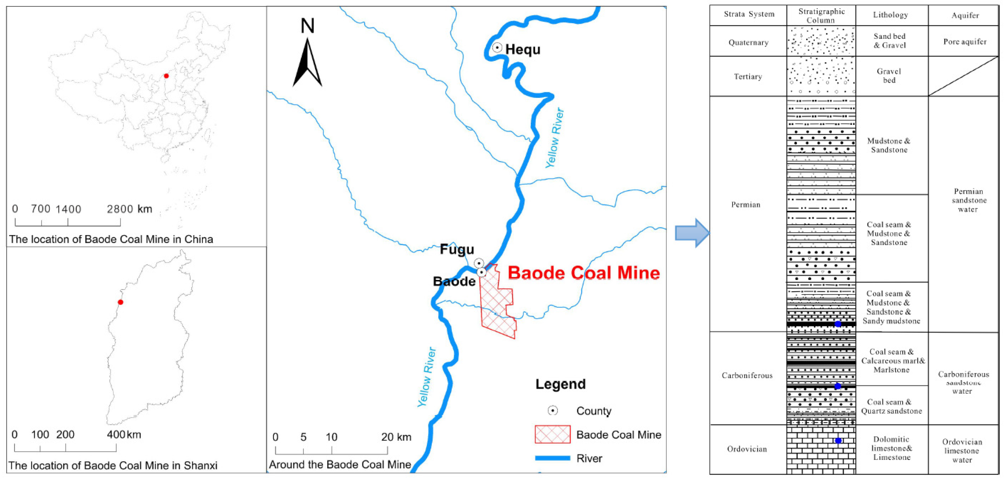
Baode Coal Mine (Figure 1) is situated in Baode County, Shanxi Province, characterized by typical North China-type Carboniferous–Permian coalfield features. The mine has an actual production capacity of 4.2 million tons per annum. The geological structure is predominantly monoclinic, with the terrain sloping from north to south towards the center, resulting in a maximum elevation difference of 335.9 m. The mine extracts several key coal seams: #8, #10, #11, and #13. The primary coal seam, #8, is found in the Permian Shanxi Formation, while seams #10, #11, and #13 are located in the Carboniferous Taiyuan Formation.

Baode Coal Mine has four primary sources of mine filling water: (1) Atmospheric Precipitation and Surface Water: This water type is classified as HCO₃-Ca-Mg, with a mineralization of 0.4 g/L. It has a limited impact on the mine’s water inflow. (2) Coal System Sandstone Fissure Water: Characterized by the HCO₃-SO₄-Na-Ca-Mg type, with mineralization ranging from 0.063 to 1.01 g/L. This water is weakly enriched in sandstone fissures both above and below the coal seams and directly contributes to the mine’s water inflow. The Carboniferous and Permian systems, consisting of mudstone, sandstone, thinly bedded marl, and coal seams, have developed inter- and intra-layer joints, creating several water-bearing layers with some hydraulic connections. (3) Ordovician Tuff Karst Water: This water is of the HCO₃-Na-Mg type and has high local chloride ion content. It is a major water-filled aquifer in the area, especially affecting the coal seams. The Ordovician tuff aquifer below the #8 and #11 coal seams is a significant water source for mining operations. Hydrogeological studies show that this aquifer is weakly to moderately water-rich, with both plane and vertical hydraulic connections. (4) Goaf water: Since there are no small kilns in the mine field, goaf water originates from the currently mined-out areas, primarily the #8 coal seam. As the goaf expands, gob water poses a potential threat to the mining of lower coal seams.

2.2. Spectral Data Acquisition

To analyze the primary water filling sources at Baode Coal Mine, researchers collected a total of 105 water samples between November 2019 and November 2020. The samples were categorized as follows: 25 samples of Permian sandstone water (marked as A), 25 samples of Permian goaf water (marked as B), 25 samples of Carboniferous sandstone water (marked as C), and 30 samples of Ordovician limestone water (marked as D). The spectral data for the water samples were obtained using the UV-1700PC UV-visible spectrophotometer system, manufactured by Shanghai Meixi Instrument Co., Ltd (Shanghai, China). This instrument covers a wavelength range of 190 to 1100 nm and has a transmittance accuracy of ±0.3% τ.

2.3. Hydrochemical Data Acquisition

In this study, we collected hydrochemical data from 54 water samples at Baode Coal Mine. The dataset includes 12 samples of Permian sandstone water, 11 samples of Permian goaf water, 16 samples of Carboniferous sandstone water, and 15 samples of Ordovician limestone water. The data consist of measurements for cations (Na⁺, Ca²⁺, Mg²⁺) and anions (HCO₃⁻, SO₄²⁻, Cl⁻).

3. Methods

The research framework for this study is illustrated in Figure 2. The process began with data enhancement and baseline correction of the spectral data. Subsequently, the water chemistry data were analyzed using a Piper trilinear plot and Pearson correlation analysis to verify their reliability. Following this, the BA-RBF machine learning model was developed and compared with three other models: GA-RBF, PSO-RBF, and RBF. Finally, the processed spectral and water chemistry data were assessed using various discriminant models to determine the most effective one. All programming and computations were conducted using Python 3.10.

3.1. Spectral Data Preprocessing

One of the primary goals of spectral data preprocessing is to select the most relevant spectral information. Unstable factors such as instrument condition, acquisition background, and detection settings can impact the consistency of spectral data. Therefore, it is crucial to apply processing techniques that are both theoretically sound and practically effective. In line with the characteristics of the spectral data collected in this study, the second-order differentiation method was employed to enhance and optimize the dataset. This method effectively addresses issues like baseline drift and smoothing background interference, improves the resolution of overlapping peaks, and increases the sensitivity of spectral lines [36]. The conversion formula is as follows:

$${\displaystyle \frac{{d^2}_y}{d_{{\lambda }^2}}}={\displaystyle \frac{{\mathrm{y}}_{\mathrm{i}+1}-{2{\mathrm{y}}_{\mathrm{i}}+\mathrm{y}}_{\mathrm{i}-1}}{{(\Delta \lambda )}^2}}$$

(1)

In the formula, y is the spectral absorbance, i = 1, 2, 3, … represents the wavelength data points, and $\lambda$ signifies the wavelength sampling point spacing.

3.2. RBF

Powell (1987) introduced the radial basis function (RBF) to address multivariate interpolation problems [37]. By the late 1980s, Broomhead and others incorporated the concept of neural network computation into interpolation processes, leading to the development of radial basis functions within the framework of artificial neural network design, thereby establishing the RBF neural network. The RBF neural network is a feed-forward network known for its local approximation capabilities, and its optimization process can be viewed as a surface fitting problem in high-dimensional space [38,39,40]. The structure of the RBF neural network is illustrated in Figure 3:

According to the topological architecture of the neural network, the input consists of the sample data matrix $X$, which includes m training samples $X_i\left(i=\mathrm{1,2}\cdots m\right)$, with each sample characterized by n attributes. The result of the output layer is Y. In this experiment, the network is fed with spectral and hydrochemical data from various types of mine water sources as input values, while the output values correspond to the types of mine water sources.

The Radial Basis Function (RBF) hidden layer employs the Gaussian function $G\left(‖x,c_i‖\right)$ as the radial basis function, and the radial distance is defined as the distance between any point x in the space and a certain center c, using Euclidean distance, denoted as $‖x-c‖$.

$$G\left(‖x,c_i‖\right)=G\left(‖x-c_i‖\right)=exp\left(-\frac{1}{2{\sigma }^2}{‖x-c_i‖}^2\right)$$

(2)

In the formula, $\sigma$ is the width of basis function, $G‖x-c_i‖$ denotes the activation function of the i-th hidden layer node, x denotes the vector of the input layer, and $c_i$ denotes the i-th center of the hidden layer. In this experiment, the values of $\sigma$ and $c_i$ are optimized by the BA algorithm. The objective function of the output layer is

$$y(x)={\sum }_{i=1}^k{w}_{i}G‖x-c_i‖$$

(3)

In the formula, $y\left(x\right)$ is the result of the output layer, k is the number of hidden layer nodes, and $w_i$ is the connection weight between the i-th hidden layer node and the output node.

3.3. BA

The Bat Algorithm (BA), is inspired by the echolocation behavior of bats during hunting. This algorithm effectively merges key features of genetic algorithms and particle swarm optimization, resulting in enhanced search and optimization capabilities. Initially, the virtual bat’s flight parameters: speed ($v_i$), position ($x_i$), pulse frequency ($f_i$), pulse loudness ($A_i$), and pulse rate ($\gamma$) are randomly assigned. As the bat detects prey, it adjusts its speed and position by varying the frequency, decreasing the loudness, and increasing the pulse emission rate. A fitness function then assesses the current position’s effectiveness, guiding the selection of the optimal solution. This forms the core concept of the BA algorithm [41].

Assuming that the size of the bat population is $m$ and the search space is $d$ dimensional, the update process of the position $x_i^t$ and the velocity $v_i^t$ of bat $i$ at time $t$ is as follows:

$$f_i=f_{min}+\left(f_{max}-f_{min}\right)\beta$$

(4)

$$v_i^t=v_i^{t-1}+\left(x_i^t-x^{\ast }\right)f_i$$

(5)

$$x_i^t=x_i^{t-1}+v_i^t$$

(6)

Among them, $f_i$ represents the acoustic frequency of bat $i$ at the current moment, while $f_{max}$ and $f_{min}$ are the maximum and minimum values of the acoustic frequency, respectively. In the whole process of bat speed and position update, the frequency of sound wave $f_i$ controls the search range of bats and plays a role in adjusting the step size. $\beta \in [0, 1]$ is a random number that obeys uniform distribution, and $x^{\ast }$ represents the current global optimal solution of the bat population.

In the local search phase, when a bat selects one of the current best solutions, it generates a new solution in its vicinity through a random walk. The updated formula for this process is

$$X_{new}=X_{old}+\epsilon A^t,\epsilon \in \left[-1,1\right]$$

(7)

Among them, $\epsilon$ is a random number, and $A^t=<A_i^t>$ is the average loudness of all bats in this generation.

Then, the loudness $A_i$ and the pulse rate ${\gamma }_i$ are also updated with the iteration process. The update formula is as follows:

$$A_i^t=\alpha A_i^{t-1}$$

(8)

$${\gamma }_i^t={\gamma }_i^0\left[1-e^{-\gamma t}\right]$$

(9)

Here, $\alpha$ and $\gamma$ are constants. When initialized, the loudness and pulse rate emitted by each bat are randomly given. In general, the initial loudness $A_i$ is usually defined between [1, 2], and the initial pulse rate ${\gamma }^0$ is generally close to 0. In the process of flying to the optimal solution, $A_i$ and ${\gamma }_i$ are constantly updated.

3.4. BA-RBF Model

The RBF neural network prediction model, optimized by the Bat Algorithm (BA), enables faster training and prediction of input data. The steps of the algorithm are outlined as follows (Figure 4):

Step 1: Determine the RBF neural network structure. Set the i-th center $c_i$ of the hidden layer and the basis function width $\sigma$ to a random uniformly distributed decimal at (0, 1). Input spectral data matrix $X$;

Step 2: Determine the BA structure and initialization parameters. Parameter initialization: bat population size $m=$ 50, number of iterations $N=$ 100; search spaced dimension = dimension of RBF input layer + 1; pulse volume attenuation coefficient $\alpha$ = 0.8, pulse rate $\gamma$ = 0.5; maximum pulse frequency $f_{max}=10$, the minimum value $f_{min}=-10$; the impulse loudness $A_i$ is a random number uniformly distributed between [1, 2] produced randomly; the values of $c_i$ and $\sigma$ are called solutions, the lower limit of the solution is $lower=-10$, and the upper limit of the solution is $upper=10$; the random initialization speed $v_i$ and position $x_i$ are also within the value range of the solution.

Step 3: Generate a new solution by frequency adjustment, and update the velocity and position according to Equations (4)–(6).

Step 4: Generate a random number, ${rand}_1$. ${rand}_1$ is a random number on [0, 1]. If ${rand}_1$ > ${\gamma }_i$, select an optimal individual among the optimal bats, and then generate a local solution near the optimal individual selected by Formula (7); otherwise, update the bat position according to Formula (6).

Step 5: Pass the obtained solution to RBF, and assign it to the hidden layer center $c_i$, the basis function width $\sigma$, and the weight w. According to the classification and recognition results, the accuracy value is calculated, and the accuracy rate is used as the fitness function. The higher the accuracy rate, the better the fitness. The fitness value is calculated and returned to BA.

Step 6: Regenerate a random number, ${rand}_2$, where ${rand}_2$ is a random number on [0, 1]. If ${rand}_2$ < $A_i$, and the fitness of the objective function is better than the new solution in step 3, then accept the position and adjust $A_i$ (reduce) and ${\gamma }_i$ (increase) by Formulas (8) and (9). Find the current best $x^{\ast }$, which, when updated, retains the optimal solution value for this generation.

Step 7: Determine whether the maximum number of iterations is satisfied, and repeat steps 3–6. Then assess output classification results and accuracy.

3.5. Model Evaluation

In this experiment, Accuracy (A), Precision (P), Recall (R), and F1 score are selected to evaluate and compare the classification performance of the RBF model, GA-RBF model (

Table 1. Parameter definition of index.

	Positive	Negative
Positive	True Positive (TP)	False Negative (FN)
Negative	False Positive (FP)	True Negative (TN)

), PSO-RBF model, and BA-RBF model. Accuracy is defined as the ratio of correctly classified samples to the total number of samples in the dataset. The other three metrics are defined as follows: typically, the class of interest is considered positive, while the other class is negative. The classifier’s prediction on the dataset can be categorized into four possible outcomes: true positive, false positive, true negative, and false negative.

$$P={\displaystyle \frac{TP}{TP+FP}}$$

(10)

$$R={\displaystyle \frac{TP}{TP+FN}}$$

(11)

$$F1={\displaystyle \frac{2P\ast R}{P+R}}$$

(12)

4. Results

4.1. Spectral Data Analysis

This study obtained a total of 105 sets of spectral data from a full scan using a UV-Vis spectrophotometer, covering the wavelength range of 190 to 1100 nm, with ultrapure water as the baseline reference. Each water sample was measured three times, and the results were averaged, with no anomalies detected. The spectral data from these tests are presented in Figure 5.

As shown in Figure 5, the maximum absorbance of Permian sandstone fissure water from Baode Mine is approximately 2.44 at 193 nm, after which the absorbance decreases. For Permian goaf water, the maximum absorbance is around 2.23 between 193 and 198 nm, with an initial increase followed by a decrease between 190 and 210 nm. In the case of Carboniferous sandstone water, the maximum absorbance reaches 3.25 between 200 and 210 nm, with a gradual change between 190 and 220 nm before decreasing. The maximum absorbance of Ordovician limestone water is about 1.99 at 193 nm, followed by a downward trend.

It is noteworthy that the absorbance peaks of the water samples are primarily concentrated in the range of 190 to 240 nm, while the absorbance values from 240 to 1100 nm tend to be less stable. Therefore, it is crucial to focus on the spectral data within the 190 to 240 nm range for subsequent spectral pre-processing and modeling.

In Figure 6, panels A, B, C, and D display the spectral data lines for Permian sandstone water, Permian goaf water, Carboniferous sandstone water, and Ordovician water, respectively, after processing the spectral data from Baode Coal Mine. Panel (a) shows the result of data enhancement, while panel (b) illustrates the result of data baseline correction. After spectral preprocessing, the overlapping peaks for each water sample have been improved, the differences between water samples have been enhanced, and the sensitivity of the spectral lines has been increased.

As shown in Figure 6, the spectrogram provides an intuitive visualization of the absorbance differences among water samples from various aquifers, facilitating the identification of different water sources. Additionally, the second derivative plot allows for a clear view of the position and magnitude of the characteristic points for each water sample.

To enhance the accuracy and speed of identifying water sources, we developed a Bat Algorithm-optimized neural network recognition model (BA-RBF). In this model, 70% of the data from the four water samples were used for training (72 samples), while the remaining 30% was reserved for testing (33 samples).

4.2. Hydrochemical Data Analysis

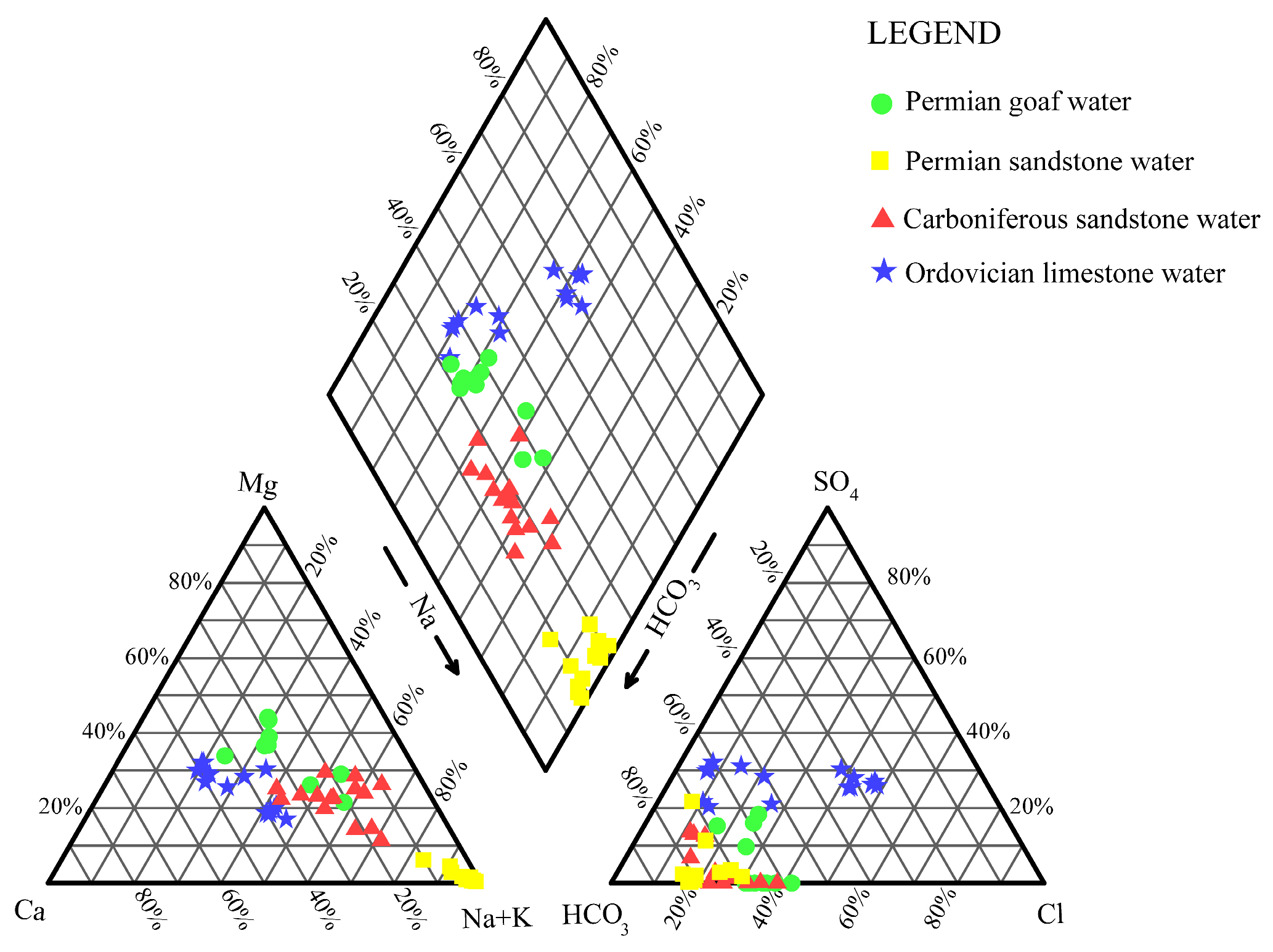
Figure 7 shows the Piper trilinear diagram, while Figure 8 presents the Pearson correlation analysis diagram for the water samples from Baode Mine.

As shown in Figure 7, the Piper trilinear diagram reveals distinct differences in water quality among the various aquifers at Baode Mine. The anion composition of the water samples from the Permian mining area is generally ordered as HCO₃⁻ > Cl⁻ > SO₄²⁻, with relatively uniform cation concentrations. In the Permian sandstone water samples, the anion content follows HCO₃⁻ > Cl⁻ > SO₄²⁻, with a notably high concentration of Na⁺, making sodium bicarbonate the dominant cation. This indicates that the water quality in this aquifer is primarily a sodium–potassium bicarbonate type. For Carboniferous sandstone water samples, the anion content also follows HCO₃⁻ > Cl⁻ > SO₄²⁻, and the water quality is predominantly a sodium–potassium bicarbonate or calcium bicarbonate type. The Ordovician chert water exhibits an anion composition of HCO₃⁻ > SO₄²⁻ > Cl⁻, with higher local Cl⁻ concentrations, consistent with geological records. This water is primarily classified as sodium–potassium bicarbonate, calcium bicarbonate, or sodium bicarbonate type. In summary, the water chemistry of samples from various aquifers is mainly classified within the bicarbonate group, with fewer samples categorized under the chloride group.

As shown in Figure 8, from the Pearson correlation analysis graph, it is evident that there are significant correlations among various ions in the water samples from Baode Mine. Specifically: Mg²⁺ and Ca²⁺ exhibit a strong positive correlation, with a correlation coefficient of 0.71. Na⁺ and HCO₃⁻ also show a strong positive correlation, with a correlation coefficient of 0.71. SO₄²⁻ and Ca²⁺ have a moderate positive correlation, with a correlation coefficient of 0.51. On the other hand, there are notable negative correlations: Ca²⁺ has a moderate negative correlation with both Na⁺ and HCO₃⁻, with correlation coefficients of −0.57 and −0.68, respectively. Mg²⁺ also shows a negative correlation with Na⁺; and HCO₃⁻, with correlation coefficients of −0.52 and −0.48, respectively. These negative correlations suggest the potential dissolution of carbonate rocks, such as calcite and dolomite, and alternating adsorption of cations. Additionally, SO₄²⁻ exhibits a moderate negative correlation with HCO₃⁻, with a correlation coefficient of −0.45. This could indicate the oxidation of sulfurous iron ore commonly found in coal seams and the alternating adsorption of cations.

Additionally, the concentrations of six ions were used as input variables, while the type of sudden water source served as the output variable. Out of the 54 data sets, 43 were selected for the training set, and 11 were used as the test set to enable the classification of sudden water sources.

4.3. Analysis of Water Inrush Source Identification Model Results

In this experiment, Accuracy (A), Precision (P), Recall (R), and F1 score were selected to evaluate and compare the classification performance of the RBF model, GA-RBF model, PSO-RBF model, and BA-RBF model. Water source discrimination was performed using three different data sets: the original spectral data (a), the second-order processed spectral data (b), and the water chemistry data (c). The computational results are presented in Figure 9.

As shown in Figure 9, the BA-RBF model demonstrates superior overall performance, with higher classification accuracy compared to the other models. The recognition accuracy of the second-order processed spectral data is notably higher. Although the original spectral data reveal differences in absorbance among water samples from various aquifers, its recognition rate is lower in RBF discrimination. Conversely, the processed spectral data yield better recognition results. Additionally, the recognition accuracy for water chemistry data is lower for the GA-RBF, PSO-RBF, and BA-RBF models compared to the spectral data. The identification model based on hydrochemical data exhibits a high misjudgment rate for Permian sandstone water (Type l), incorrectly classifying a significant number of Permian sandstone water samples as Carboniferous sandstone water (Type 3). This may be attributed to the similar hydrochemical composition and closely related water quality types of the water samples from these two aquifers.

The original spectral data, second-order processed spectral data, and water chemistry data were each used with the BA-RBF model for water source discrimination. The error plots for the training set and test set are shown in Figure 10. In these plots, yellow triangles represent the actual categories of water samples, while blue pentagrams indicate the results of the discrimination. When the actual categories and the discriminated categories match, the yellow triangles and blue pentagrams overlap in the same position on the figure. Overlap is expected if the training set contains a larger amount of data, which is a normal occurrence.

From Figure 10, it is evident that the BA-RBF model achieves a discrimination rate of approximately 96.97% using both the original spectral data and the second-order processed spectral data. However, the training accuracy does not reach 100%. This may be related to data noise and the complexity of hydrogeological conditions.

In the discrimination result graph shown in Figure 9, the BA-RBF, PSO-RBF, and GA-RBF models were each subjected to 100 iterations of optimization search. The corresponding fitness curves are illustrated in Figure 11.

According to Figure 11, the fitness value of the BA-RBF model throughout the iteration process outperforms the other two classification models. It reaches the maximum accuracy value and stabilizes when the number of iterations is fewer than 10, demonstrating the best convergence effect. The GA-RBF model also converges around 10 iterations but exhibits slight fluctuations until it stabilizes at approximately 55 generations. The PSO-RBF model stabilizes around 80 generations, but its classification performance is relatively poor. Thus, the optimal value achieved by the BA-RBF algorithm is closest to the actual optimal value of the function.

In summary, the comparison of classification values with true values and the analysis of error results show that the PSO-RBF model, without any preprocessing, has the worst discrimination ability. The BA-RBF model, with its closer alignment to the true values and superior discrimination performance, outperforms both the GA-RBF and PSO-RBF models, which are themselves better than the RBF model. The recognition rate of the BA-RBF recognition model based on processed spectral data reached 96.97%, which was significantly better than that of the hydrochemical recognition model that has been widely studied and applied in recent years.

5. Conclusions

To ensure reliable prediction of mine water emergencies, this paper establishes a rapid discrimination model for mine water sources using the BA-RBF algorithm. This model integrates spectral data of water samples with hydrochemical data, while accounting for geographic and environmental factors. The BA-RBF water source identification model was then applied to the Shanxi Baode Coal Mine. Based on the analysis of water samples from four different aquifers in the mine, the following key conclusions were drawn:

(1) Measuring the absorbance of water samples using a spectrophotometer allows for the rapid creation of sample datasets. With sufficient water sample data, this method can effectively build a spectral database that enhances source identification, particularly in mining areas with complex geological conditions;

(2) The BA-RBF model developed for identifying water inrush sources in this research offers advantages such as rapid processing speed, high accuracy, and minimal sample volume requirements. It achieves predictive accuracy of up to 96.67% for both raw spectral data from different aquifer samples and spectral data that have undergone baseline correction and noise reduction;

(3) A comparison of the prediction accuracy for four different models—RBF, GA-RBF, PSO-RBF, and BA-RBF—was conducted using spectral data from various aquifers. The analysis revealed that the BA-RBF model had the highest recognition accuracy. This model significantly aids in the swift identification of water surge sources and helps mitigate disaster losses in similar mining areas;

(4) Compared to traditional water source identification methods that rely solely on hydrochemical data, the effectiveness of the water source identification approach based on spectral data has been demonstrated.

This study introduces a novel method for identifying sudden water sources. However, due to the constraints of the current research, only one water source identification method was explored. Future research should focus on developing and applying more comprehensive methods for identifying water sources in mixed water conditions. In addition, in future research, endeavors can be made to integrate spectral data with a broader array of technical approaches, such as travel-time tomography technology [42,43]. It is imperative to amass more data from diverse coal mines and enhance long-term monitoring of water samples. This will enable a more in-depth exploration of the model’s robustness, resilience, and scalability in a dynamic environment.