Discrimination of Spatial and Temporal Variabilities in the Analysis of Groundwater Databases: Application to the Bourgogne-Franche-Comté Region, France

Abstract

This study highlights the importance of distinguishing the mechanisms driving spatial and temporal variances in groundwater database analyses, with a particular focus on bacteriological contamination processes. Groundwater quality data from the Bourgogne-Franche-Comté region of France forms the basis of this investigation. Specifically, the SISE-EAUX database includes 3569 groundwater samples collected over various dates from 989 monitoring points. The methodology involves structuring the data into three distinct sets: (1) A spatio-temporal dataset without any conditioning; (2) A spatial dataset that assigns the mean values of each parameter to each sampling point; (3) A temporal dataset that captures deviations from the mean for each sampling point and parameter. These datasets enable a separate analysis of spatial and temporal variances. Principal component analysis (PCA) and parameter hierarchical clustering were used to compare the results, yielding valuable insights into the underlying processes. This analysis helps distinguish between factors related to geological or pedological spatial distributions and those associated with climatic events, such as intense rainfall episodes exhibiting seasonal patterns. Such differentiation enhances the understanding of fecal contamination vectors and nitrate pollution, which are often linked to surface and subsurface runoff in vulnerable catchment areas. While conceptually clear, the practical separation of spatial and temporal variability presents challenges. For example, catchments sensitive to surface water inflows during rainfall events are unevenly distributed across the region, correlating with specific natural environments. As a result, areas of high temporal variability are also well-structured spatially, underscoring the interdependence of these two types of variability. This complexity is exemplified by the behavior of iron, which varies in association with surface and subsurface parameters depending on spatial and temporal contexts. Additionally, asynchronous sampling and varying frequencies across sites lead to discrepancies in the average temporal data acquisition between points. These disparities can influence spatial variability calculations, as temporal variability effects are not entirely removed. Despite these challenges, the distinction between spatial and temporal components is essential for a deeper understanding of groundwater quality mechanisms. This refined approach improves diagnostic precision and supports more targeted and effective water resource management strategies.

1. Introduction

Groundwater constitutes a major proportion of water intended for human consumption for several reasons. It is often of good quality and requires less treatment than surface water, making it a valuable resource [1,2,3,4,5,6]. Unlike surface water sources (rivers, lakes), which can be subject to seasonal fluctuations or extreme weather conditions, groundwater provides a more stable and reliable resource. Due to natural filtration through layers of soil and rock, it is often less exposed to surface contaminants (bacteria, heavy metals, chemicals) [7]. In some cases, it is the only water source available for rural and remote communities. However, as it is “invisible” [8], sustainable resource management across vast regions requires an essential understanding of its characteristics, both quantitative and qualitative. In this context, the existence of large databases can prove to be an effective analytical tool [9,10] for understanding the origin of these characteristics, even though the integration of data from different original studies, encompassing diverse properties or resource characteristics (hydrochemistry, water resources, recharge, etc.), are often lacking [10,11]. This is especially unfortunate as acquiring water quality data at a regional scale requires significant and costly fieldwork and laboratory analysis.

While in many countries the management of groundwater is entrusted to respective geological surveys, in France, water quality monitoring has been assigned, as part of sanitary control, to health agencies that have been maintaining a national database for over 40 years. In total, more than 33,500 water catchments are used to supply drinking water to the population, 96% of which rely on groundwater. This corresponds to an average density of one catchment per 16 km², monitored more or less regularly [12,13]. The database thus generated exhibits spatial variability, influenced by numerous factors (lithology, topography, human land use), as well as temporal variability (seasonality, agricultural practices, weather events). The data collection spans several years to several decades, with all sampling efforts not being synchronized. As a result, analyzing the information contained in such databases can be complex. To the best of our knowledge, a separate analysis of spatial variability and temporal variability, to identify the mechanisms associated with each of these aspects, has never been thoroughly addressed.

Fecal contamination is the primary factor for non-compliance of water intended for human consumption, and recent studies based on regional extractions from the SISE-EAUX database identify it as a significant source of variability [14,15,16,17,18,19,20]. These studies have highlighted that bacterial contamination is associated with multiple factorial axes in multivariate analyses, suggesting the presence of several mechanisms that may not be solely explained by the commonly acknowledged pathway: “heavy rainfall > runoff and germ transport > contamination of the most vulnerable catchments”. While this mechanism is widely recognized [21,22,23] and often presented as the sole explanation, high contamination levels are typically linked to waters with lower mineralization due to dilution effects from rainfall. Some of these works address spatial and temporal variance, but only to quantify the information loss that accompanies grouping into homogeneous groundwater bodies for optimized resource management within a multi-parameter mapping strategy. The mechanisms specifically responsible for spatial and temporal variability have not been investigated in detail.

This study is based on data extracted from the SISE-EAUX database at the regional scale of Bourgogne-Franche-Comté (BFC, France). Its objective is to examine the mechanisms driving spatial, temporal, and spatio-temporal variability in groundwater quality, with a particular focus on the processes leading to bacteriological contamination.

2. Materials and Methods

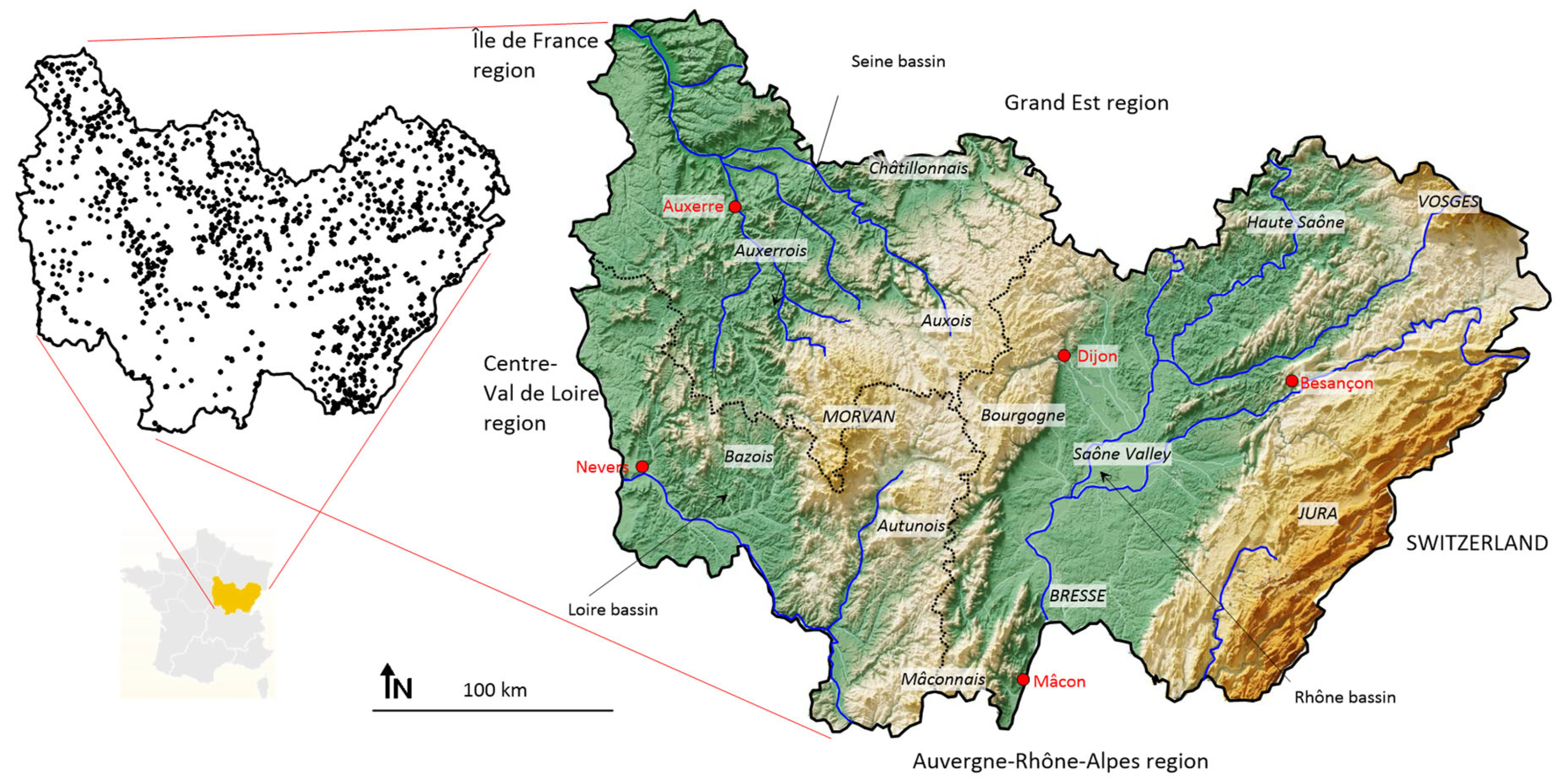
2.1. Study Area

The Bourgogne-Franche-Comté region, located in east-central France (Figure 1), consists of eight administrative departments: Côte-d’Or, Jura, Haute-Saône, Nièvre, Yonne, Saône-et-Loire, Territoire de Belfort, and Doubs. Covering an area of 47,784 km², it is the fifth-largest administrative region in France. It spans three major river basins: the Seine, the Loire, and the Rhône. The region’s elevation ranges from the Saône plain and the Seine valley (~170 m) to the peaks of the Vosges (1247 m) in the northeast and the Jura (1495 m) in the east. The Morvan Massif (901 m) occupies the central part of the region. Bourgogne-Franche-Comté is bordered by the Centre-Val de Loire region to the west, Île-de-France to the northwest, Auvergne-Rhône-Alpes to the south, Grand-Est to the north, and Switzerland to the east.

The region is composed of three major structural domains:

• The Hercynian Massifs, composed of metamorphic and crystalline rocks (schists, gneisses, granites) forming the bedrock of Bourgogne, the Morvan, and the southern Vosges. These rocks have been eroded over time, providing the materials accumulated in lower areas;
• The Mesozoic Domain, mainly consisting of sedimentary rocks (limestone, chalk, marls) formed on the flattened Hercynian bedrock in shallow seas. These sedimentary deposits can be observed on the plateaus of Bourgogne, Haute-Saône, Auxois, Bazois, and the Jura Massif. The Jura Massif itself was formed 35 million years ago through compression from the Alpine orogeny pushing westward;
• The Cenozoic Domain, created after the sea retreated and the Saône Rift was formed. It consists of materials transported by rivers descending from elevated zones and is covered by glacial deposits laid during major glaciations.

For more details on the geology and, more broadly, the diversity of the region, readers are encouraged to refer to previous studies [24].

2.2. SISE-EAUX Database Extraction

SISE-EAUX is a groundwater quality database managed by the French Ministry of Health and its regional and departmental agencies (ARS). It is designed for the organized storage of health-related water information [25,26] and has been operational since the 1990s. The study is based on an extraction of data from this database covering the entire administrative region of Bourgogne-Franche-Comté over a period of 5.4 years, from 11 January 2016 to 25 May 2021 (https://data.ofb.fr/catalogue/data-eaufrance/eng/catalog.search#/home, accessed in March 2023). All analyses were performed by ARS-accredited laboratories with international accreditation and analytical quality certification. Only raw water samples—collected from abstraction points and untreated for potability—were included in this study. The number of parameters analyzed for each water sample varies depending on the type of analysis: routine monitoring (basic physico-chemical parameters such as major ions and fecal bacteriology), targeted analyses, or more comprehensive analyses, such as those performed during an initial sampling (up to a hundred parameters, including pesticides, metals, metalloids, trace elements, and full bacteriology). As a result, the data extraction produced matrices containing numerous empty cells, referred to as sparse matrices. The sparse matrix resulting from the regional data extraction contains 8723 observations and over 100 parameters. After manually correcting data entry errors and removing empty cells, a complete matrix with 3569 observations and 22 parameters was selected for this study. These 22 parameters include electrical conductivity at 25 °C (EC), fecal bacteriology indicators (Enterococcus and Escherichia coli, labeled as Enter. and E. coli), major ions (Na⁺, Ca²⁺, Mg²⁺, Cl⁻, SO₄²⁻, HCO₃⁻, NO₃⁻, NH₄⁺), metals and trace elements (Fe, Mn, B, F, As, Se, Cd, Ni), total organic carbon (TOC), and turbidity (Turb.). For clarity, the distinction is made between a parameter (e.g., SO₄) and the corresponding ion (e.g., SO₄²⁻). The distribution of the study’s sampling points is shown in Figure 1. The complete matrix includes data from 989 sampling points, with between 1 and 12 samples collected, resulting in an average of 3.6 samples per sampling point during the extraction period. Where several aquifers are superimposed, only the most superficial aquifer has been retained.

2.3. Data Treatments

2.3.1. Data Conditioning

To limit the influence of extreme values [27,28], which could obscure important mechanisms during data processing, the data were subjected to a logarithmic transformation using the formula y = log10(x + DL), where x represents the value of the parameter X (physico-chemical or bacteriological) and DL is its detection limit.

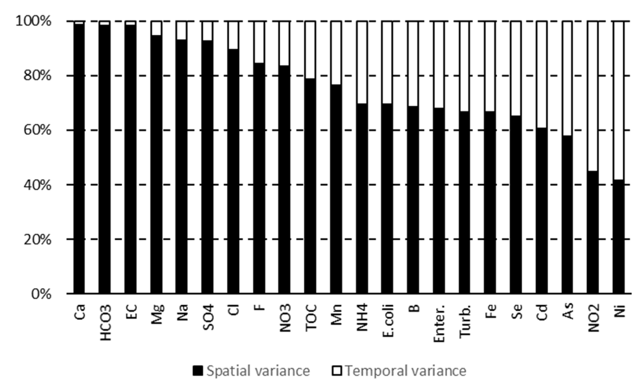
2.3.2. Separation of Spatial Variations and Temporal Variations

The spatio-temporal dataset consists of all the data from the full matrix, i.e., 3569 observations and 22 parameters. Over the period covered by the extraction, the database contains multiple analyses for each of the sampling points (Figure 1). Therefore, the variance includes both temporal variability, reflected by different values at the same sampling point, and spatial variability, reflected by different averages between sampling points. On one hand, a spatial dataset was created by assigning to each sampling point the mean values of each parameter (989 observations and 22 parameters). On the other hand, the calculation of the deviation from the mean for each sampling point and for each parameter creates a dataset (centered around zero) representing the temporal variability at each point (989 observations and 22 parameters). These zero-centered data were then merged, meaning that all the temporal variabilities from all the sampling points were overlaid in order to study the spatial structure of the temporal variability of each parameter.

2.3.3. Analysis of Variance

An analysis of variance (ANOVA) was performed using water characteristics as the dependent variable, and the “sampling point” criterion as the non-quantitative explanatory variable [29], thus providing the spatial variability [30]. The variance explained by each parameter was measured by the R² [31,32], according to the following formula:

R² = 1 − (RSS/TSS),

(1)

where RSS is the residual square sum and TSS is the total square sum of the values of each parameter. R² represents the percentage of spatial variance explained by its relationship with the explanatory variables. The complement to 1 of R² represents the fraction of unexplained variance [33] and reflects the temporal variance of each parameter, to which a small portion of variance due to analytical imprecision is added, which will be disregarded.

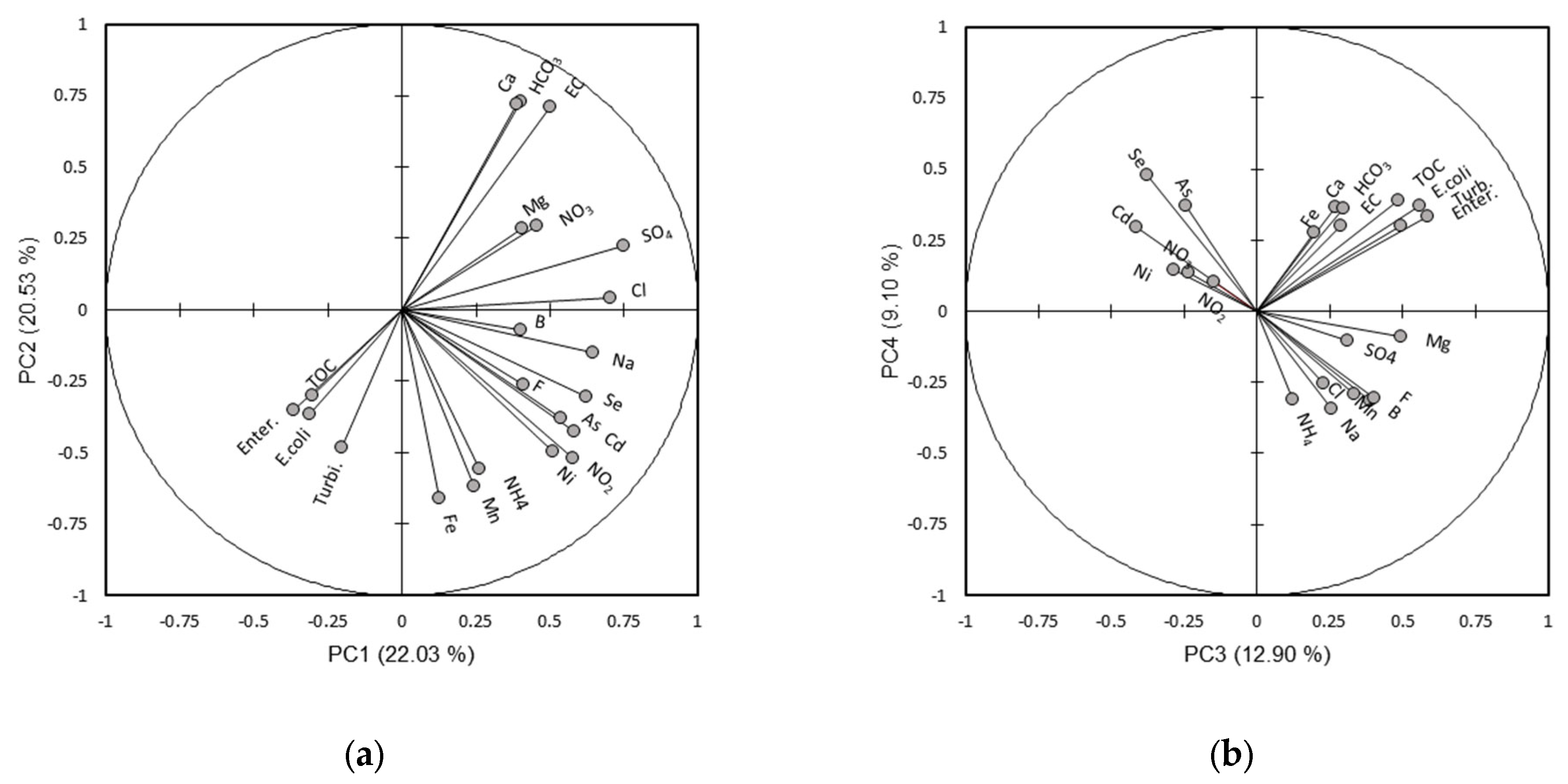
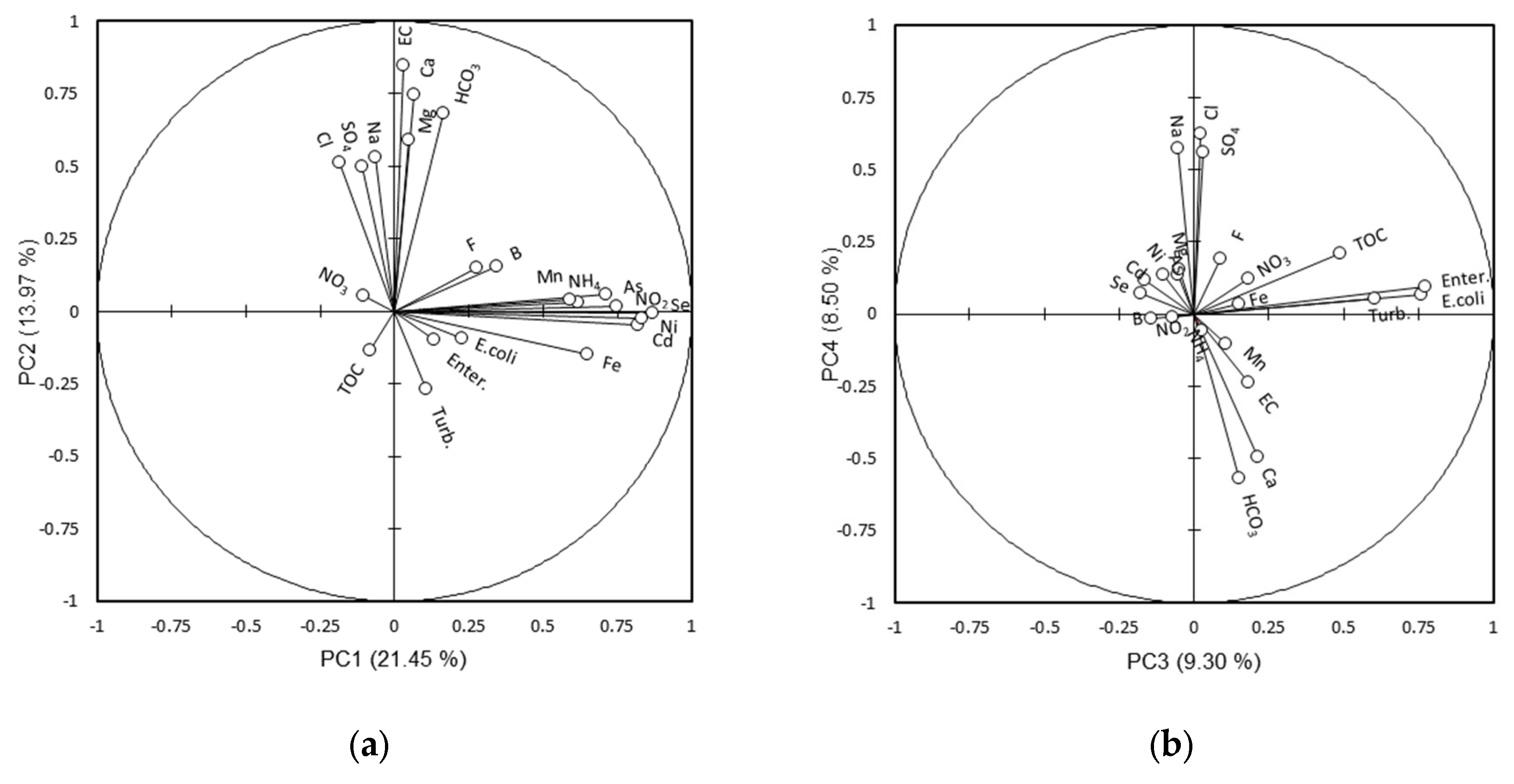
2.3.4. Principal Component Analysis

A principal component analysis (PCA) was conducted on the full matrix of log-transformed data to identify and rank the sources of water quality variability as well as the mechanisms associated with them. Analyses from the three full matrices (spatio-temporal, spatial, and temporal) were compared. The PCA was performed using the correlation matrix. Under these conditions, the identified factor axes are orthogonal and represent independent processes [34].

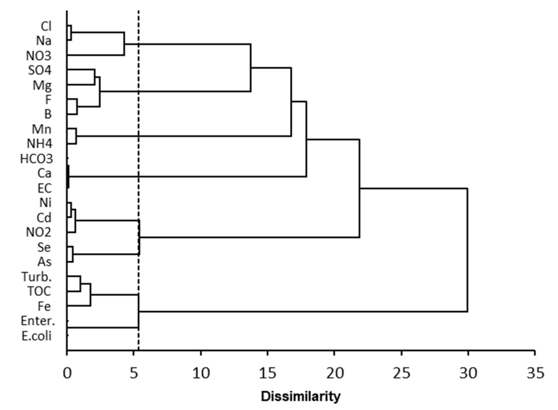
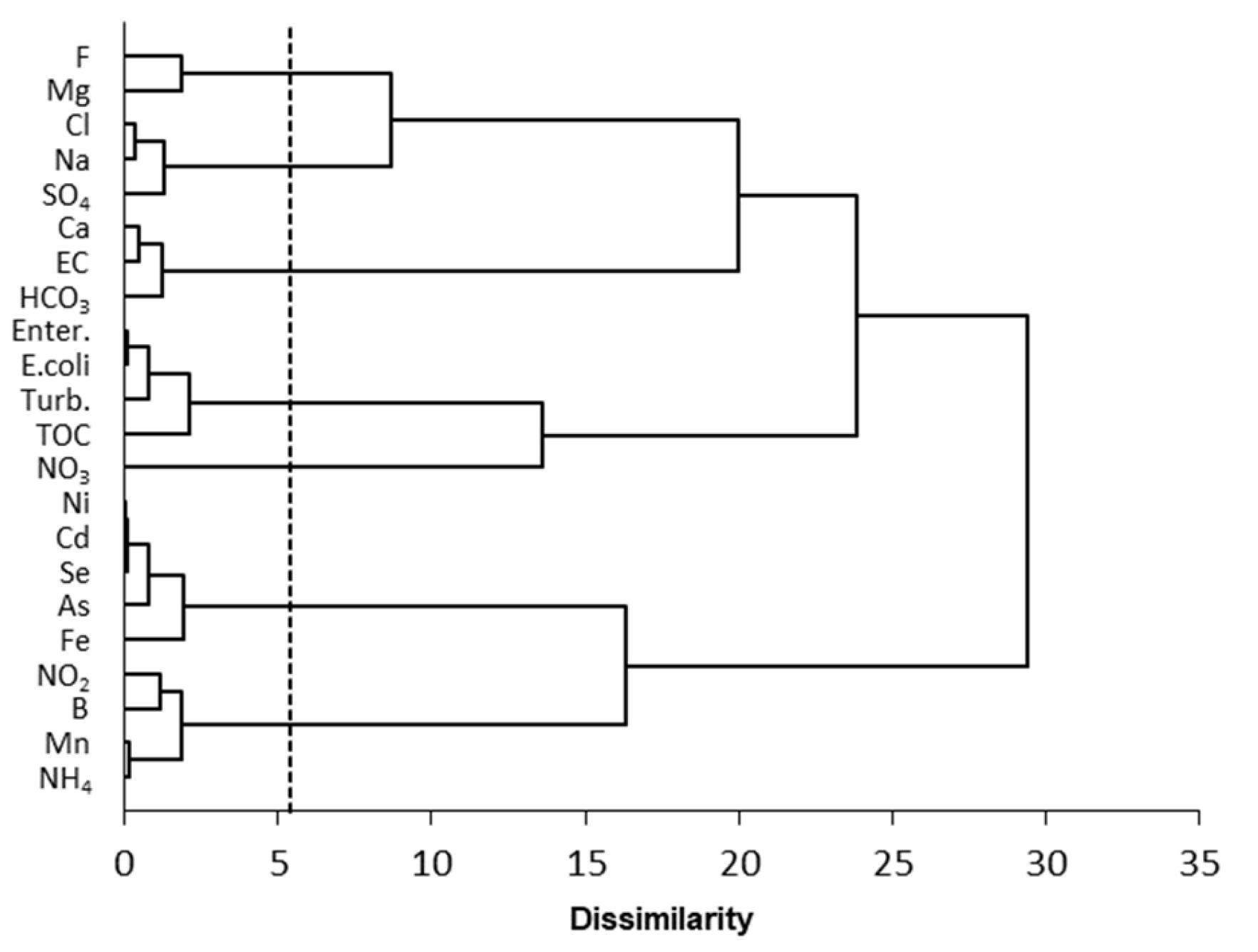
2.3.5. Parameters Hierarchical Clustering

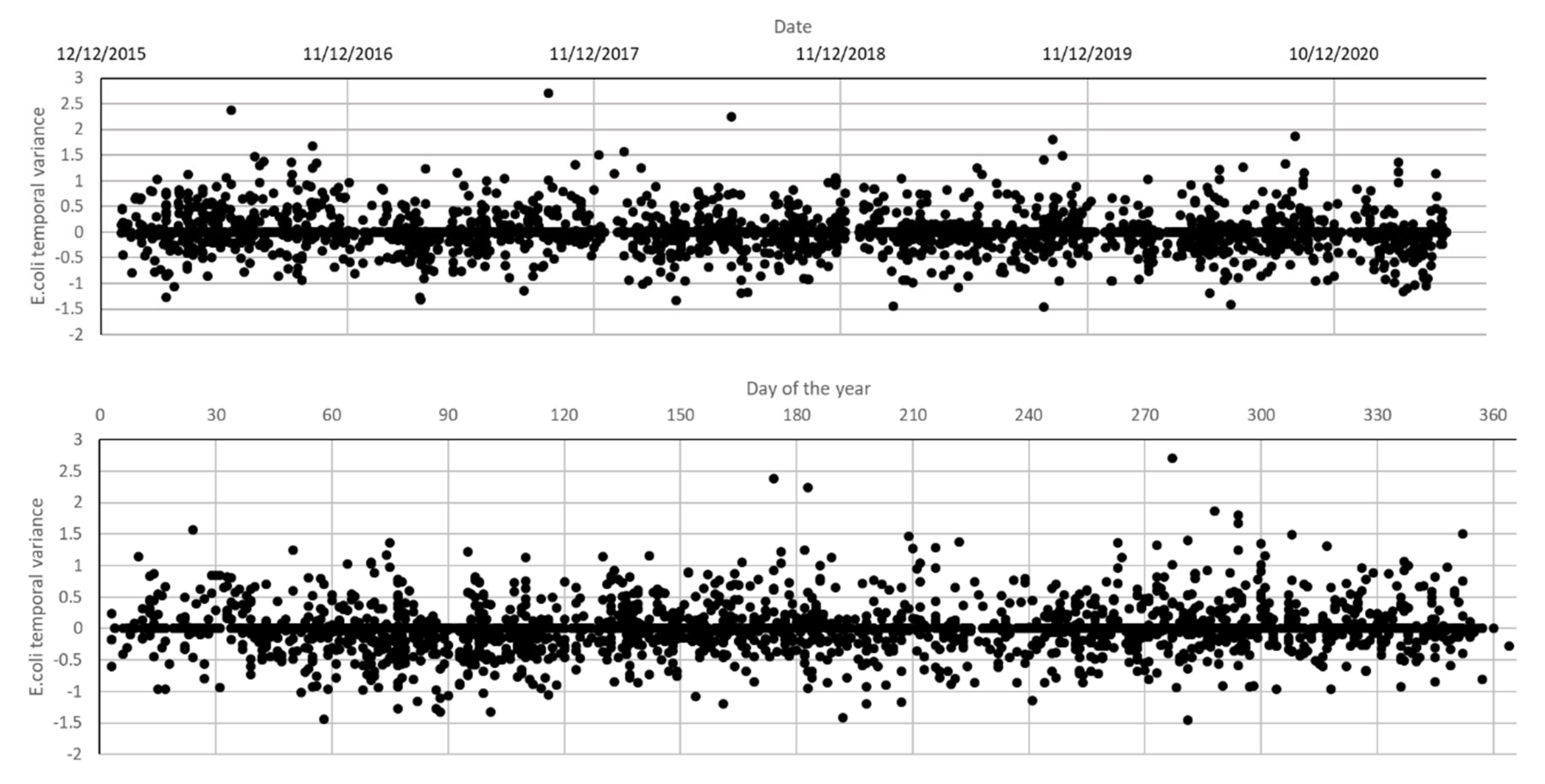
In order to compare the behavior of the different parameters, they were grouped using unsupervised hierarchical clustering [35] according to three modalities. The first is based on the coordinates of the parameters on the main factor axes, meaning the grouping was made according to the correlational information between the parameters. The second modality was conducted based on the mean of each parameter at the sampling points (i.e., based on spatial variability), while the third was based on the deviation of the analytical results from the mean, i.e., based on temporal variability. These three types of grouping address the classification of water quality parameters according to different criteria. For each processing, the first eight factor axes were considered.

2.3.6. Seasonality

In order to compare the temporal variability across all the sampling points, the analysis results for each parameter were normalized by the mean of that parameter at the corresponding sampling point. This effectively centers the values around the local mean, so the result reflects only the local temporal variability. These data were used, on the one hand, to assess the trends in temporal variance over the entire period for each parameter, and on the other hand, to analyze the seasonal variance over the 5.4 years of the dataset.

2.3.7. Spatialization of Temporal Variance

Temporal variations were calculated by subtracting the local mean to each value. Therefore, the sum of the deviations for each sampling point is zero. To map temporal variance, the values were squared, which is consistent with a variance. Indeed, the map calculation averages the different values obtained at the same sampling point, which amounts to mapping temporal variance. Consequently, mapping temporal variability involves mapping the temporal variance at each sampling point.

3. Results

3.1. Spatio-Temporal Data

The analysis of variance indicated a spatial variance proportion ranging from 42% to 99% of the total variance, depending on the parameter (Figure 2). As a consequence, the temporal variance ranged from 1% to 58% of the total variance. For major ions and electrical conductivity, the variance was primarily spatial, with negligible temporal variance. In contrast, for bacteriological parameters and especially trace elements, the proportion of temporal variability was significant, while spatial variability was lower.

The inertia of the factor axes from the PCA showed that the information contained in the dataset was distributed across many axes, reflecting a great diversity of variability sources and thus complex information (Figure 3). The first six principal components had eigenvalues greater than one, meaning they concentrated more information than a single initial parameter. The first four factor axes accounted for between 22% and 9.1%, cumulatively representing 65% of the information, considering all water samples and parameters.

The first factor axis was positively scored with chlorinated-sulfated sodium and rather mineralized waters, characterized by the presence of various forms of nitrogen, heavy metals, and arsenic (Figure 4a). In contrast, the most diluted waters were marked by fecal contamination. The second factor axis, however, contrasted waters with higher minerality and a more calcium-carbonate chemical profile to the most diluted waters, characterized by fecal contamination and heavy metals. It should also be noted that the most diluted waters were associated with nitrate, the oxidized form of nitrogen, while the most mineralized waters were marked by ammonium and nitrites, typical of reducing waters. These results suggest that the most diluted waters correspond to infiltration of surface waters, marked by higher turbidity and TOC content, such as runoff waters during rainfall events, while the most mineralized waters were more indicative of non-surface, anoxic waters. Fecal contamination played a major role in the third factor axis (Figure 4b). It was not associated with the most diluted waters, as seen in the first two principal components, but with the most mineralized waters, still marked by turbidity and TOC, low in nitrate and metals except for Fe and Mn, which are here surface markers. Like the third axis, the fourth factor axis linked fecal contamination, turbidity, and TOC to the most mineralized waters, but here with a calcium-carbonate profile. These last two factor axes thus reflected lithological opposition.

These results led to a typology of the parameters based on the first eight principal components, represented by the dendrogram in Figure 5. The parameters E. coli and Enter. were strongly correlated and connected to the group Turbidity, TOC, Fe. This set of five parameters, characteristic of surface waters, was completely distinct from all other parameters. The metalloids As and Se, along with the metals Cd and Ni, formed, with nitrites, another group of parameters that also stood out from the rest. Ca, HCO₃, and EC formed a third well-defined group. A fourth group consisted of the parameters Mn and NH₄, characteristic of more reducing environments. Finally, the last, more heterogeneous group was composed of the other water quality parameters.

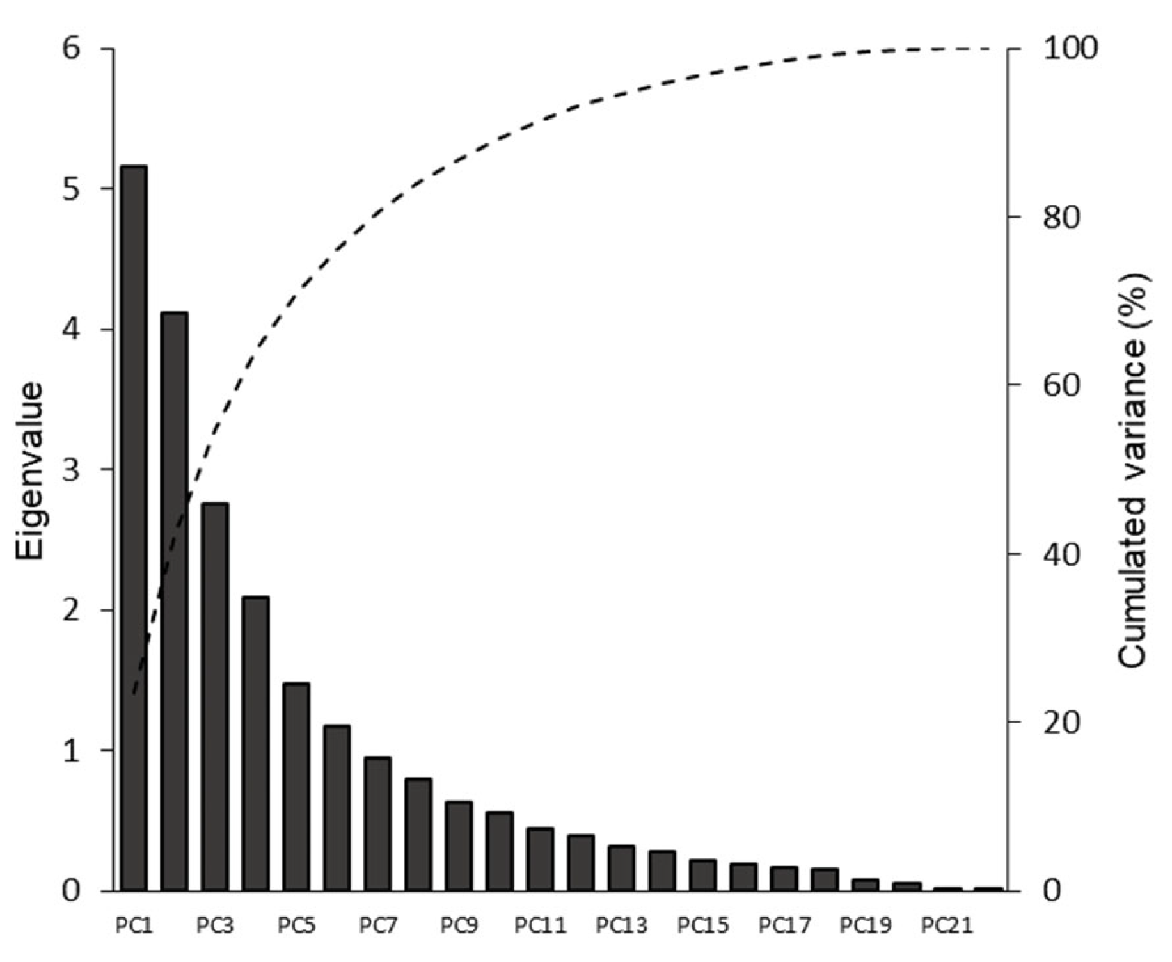
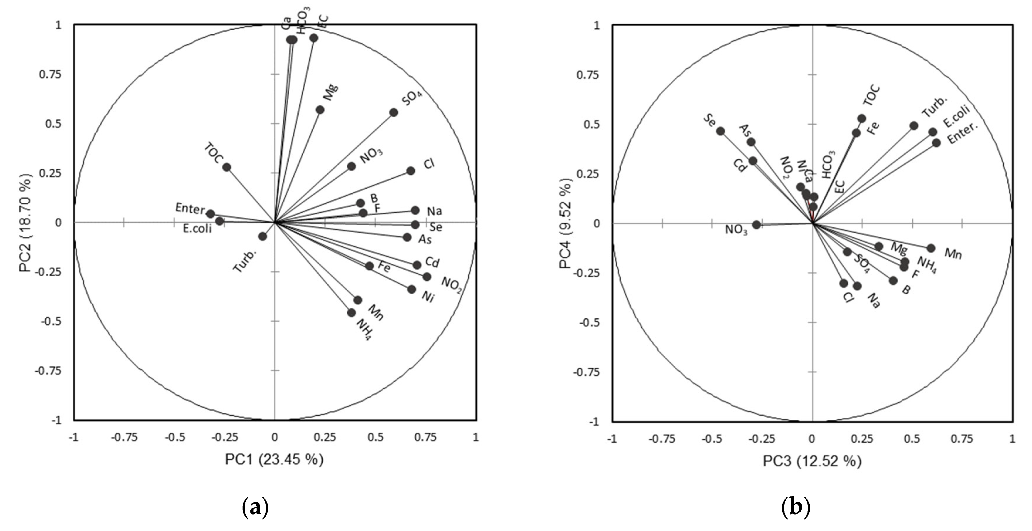
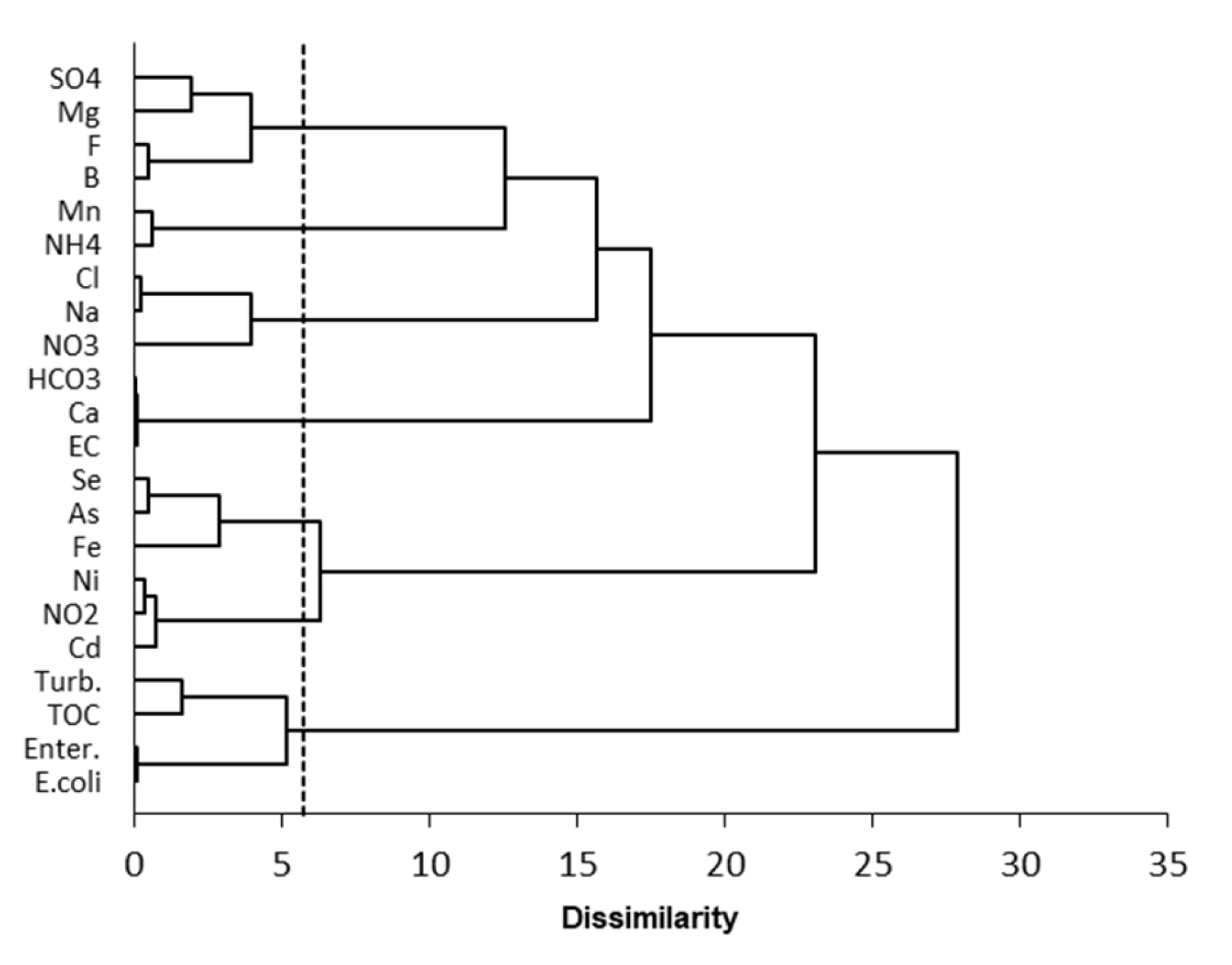
3.2. Processing of the Spatial Data Matrix

These data represent the local averages, that is, the averages for each sampling point. The full matrix used contains 989 sampling points for which the 22 previously mentioned bacteriological and physico-chemical parameters were considered. As expected, due to the low share of temporal variance for most water quality parameters, the distribution of the inertia of the principal components along the different factor axes was very similar to that observed for the spatio-temporal data (Figure 6).

The first factor axis (23.5% of the variance) contrasted waters contaminated by Escherichia coli and Enterococci, marked by TOC, with chlorinated sulfate-sodium waters marked by the presence of various nitrogen forms, heavy metals, and associated metalloids (Figure 7). Thus, there was a clear lithological component conveyed by this first principal component (PC). The second factor axis (18.7% of the variance) contrasted the most mineralized waters with a calcareous-sulfate magnesium-calcium chemical profile, with waters rich in metals, metalloids, and nitrites. Similarly, this axis conveyed a redox component associated with different lithologies and pedologies. The third factor axis contrasted waters contaminated by E. coli and Enter., marked by turbidity, Mn, Fe, B, F, and NH₄, with waters rich in Se, Cd, and NO₃. This opposition was both lithological and characterized by redox features. This PC3 accounted for 12.5% of the variance. The fourth factor axis (9.5% of the total variance) showed an opposition between turbid surface waters with high metal content and deep waters.

The parameter typology obtained through clustering was quite similar to that obtained from the spatio-temporal variations, with a notable difference concerning iron (Figure 8). In the case of spatio-temporal variations, iron was associated with turbidity, TOC, and bacteriological parameters. However, in the spatial matrix analysis, it was associated with metals and metalloids (As, Se, Ni, Cd) and nitrites.

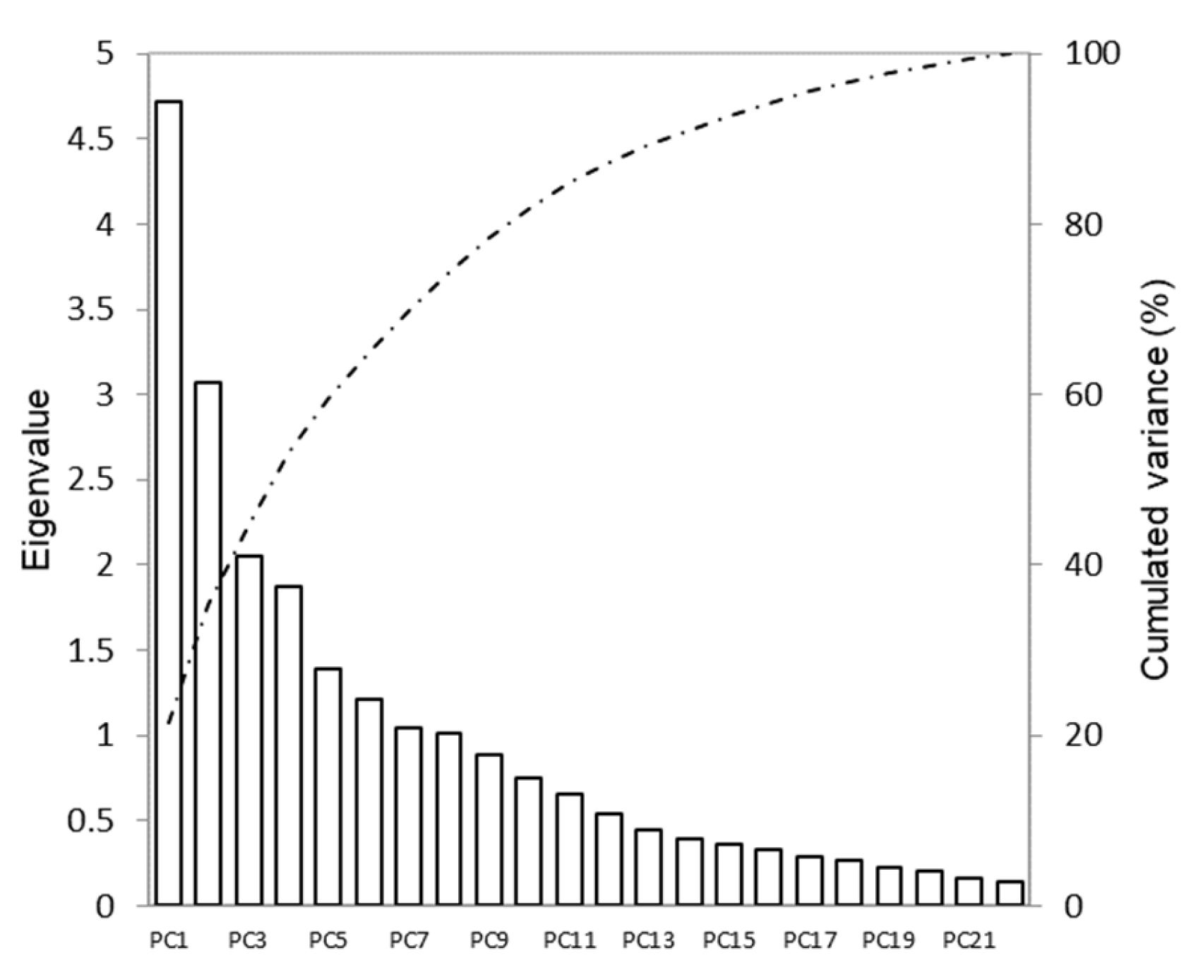
3.3. Processing of the Temporal Data Matrix

The matrix contains 3569 sampling points and 22 parameters. The processed data represent the differences from the local means in logarithmic units. The information was spread across more axes than in the previous treatments, with the first eight principal components (PCs) having eigenvalues greater than one (Figure 9). The first PC (21.5% of the variance) opposed, on one side, the compounds, stable in a reducing environment, and on the other side, the nitrates, stable in an oxidizing environment. It could represent the opposition between older waters (reducing, stagnant in some environments) and more aerated waters, recently arrived in the environment (Figure 10a). The second factor axis (14% of the variance) represented the opposition between the most mineralized waters and waters with lower ionic load, turbid, marked by suspended solids (Turb), total organic carbon (TOC), and colloidal iron, and positively scored with the bacteriological parameters. It most likely reflected the effect of contamination of catchments by runoff waters during storm events. The low weight of bacteriological parameters and the weak but negative correlation of these parameters with nitrates, however, seems to indicate a medium that is not highly exposed to slurry and manure spreading. The third axis represented surface waters with a tendency toward calcareous areas. It also reflected the contamination of catchments by runoff waters, but for environments more exposed to nitrogen fertilization (agriculture) and the spreading of manure and slurry compared to axis 2. The fourth axis clearly opposed two distinct chemical profiles: on one side, the Jurassic calcareous areas (Ca, HCO₃, and EC), and on the other side, the Triassic areas marked by Na, Cl, and SO₄.

The typology of parameters based on temporal variability showed a much closer relationship between the bacteriological parameters, turbidity, and TOC than with the spatial or spatio-temporal data treatments, resulting in a very low dissimilarity. Nitrate was grouped with this set, although with a notable dissimilarity (Figure 11).

3.4. Seasonality and Trends over 5.4 Years

At the temporal level, there was no seasonal trend or trend over the sampling period (5.4 years) in the evolution of major ions and electrical conductivity. This lack of trend for these physico-chemical parameters is consistent with their low temporal variance (Figure 2). Similarly, no clear trend over 5.4 years was detected for the bacteriological parameters (Figure 12). However, when displaying the bacteriological data by day of the year, across all years, a slight seasonal trend is observed, with two maxima occurring in early summer (second half of June) and in autumn (September 15 to November 10).

3.5. Spatialization of Temporal Variance

The distribution maps of the temporal variance are presented in Figure 13 for a few parameters. The maps showed a non-random distribution of temporal variance. Generally, areas of low temporal variability were located in the northern central part of the region, but there were notable differences depending on the parameter. For instance, areas where NO₂ showed temporal variations (southern to southeastern part of the region) were very different from those where electrical conductivity varied over time (southwestern edge).

4. Discussion

4.1. Overview of the Datasets

The spatial dataset was designed to eliminate most of the temporal variability by assigning the average value calculated for each parameter and sampling point. However, since collections were not synchronized across all sampling locations, a small portion of temporal variance remains, which was deemed negligible for this study. Furthermore, the extent of temporal variance depends significantly on the number of samples per sampling point. It is easy to understand that if there is only one analysis per location, the temporal variability is null (or nearly null, considering that the samplings are not synchronized across different sites). Conversely, if the database contains numerous samples for each site over the extraction period considered, temporal variance will be significant. In our case, we recorded an average of 3.6 samples collected per sampling point (3569/989), a low ratio that therefore reduces the influence of temporal variability in this dataset. Increasing this ratio would likely amplify the proportion of temporal variance compared to the spatial variance, but would not affect the differentiation between the various parameters, as all parameters pertain to the same samples. Thus, comparing different parameters remains meaningful in terms of the relative importance of temporal variability. Since the variance calculations for spatio-temporal, spatial, and temporal variances were performed on the same dataset, similarities exist in the results obtained. In what follows, only differences and key highlights will be emphasized and analyzed.

One consequence of the low proportion of temporal variance for many parameters is that the distribution of inertia among principal components in the analysis based on spatial variance closely resembles that observed in spatio-temporal data (Figure 3 and Figure 6). Temporal variability is high for microbiological parameters and trace elements but low for the physico-chemical parameters of major ions (Figure 2). This result aligns with findings from other regions, such as Provence-Alpes-Côte d’Azur, Occitanie, or Auvergne-Rhône-Alpes [16,18,27].

4.2. Pathways of Fecal Contamination in Groundwater

This study clearly demonstrates that runoff and the transport of bacteria via particles (clay, organic matter, and colloidal iron) are the major processes leading to aquifer contamination. In most studies dealing with the analysis of datasets from groundwater, which inherently include a mix of spatio-temporal variance, the first factorial axis—representing a major source of variability—opposes the most diluted water contaminated by E. coli and Enterococci to the most mineralized, non-contaminated water. The grouping of E. coli-Enterococci, on one hand, and electrical conductivity (EC) on the other, shows a marked opposition, with one contributing strongly positively and the other strongly negatively to the first factorial axis [16,18,19,20,24,27,28]. This is also observed in the present study (Figure 4), where the first two factorial axes oppose more diluted to more mineralized water, with variables such as turbidity, total organic carbon (TOC), and fecal contamination associated with diluted water. This opposition disappears in the case of spatial analysis, with bacteriological parameters contributing significantly only to the third and fourth principal components (PCs) and without a marked opposition to ionic load. However, the opposition persists in temporal variance analysis, though it appears in the second position, following a first PC reflecting seasonal redox processes. Groundwater contamination by fecal-origin bacteria thus exhibits a strong seasonal temporal component (Figure 12). In parallel, the clustering of parameters by similarity confirms that bacteriological parameters are much more clearly associated with turbidity and TOC (with very low dissimilarity) in the temporal variance treatment compared to other approaches (i.e., maximizing spatial variance or analyzing the entire dataset). Nitrate is grouped with this cluster but with some dissimilarity, indicating the contribution of hypodermic runoff associated with surface runoff, marked by turbidity and bacteriological parameters. The most sensitive areas appear to be environments moderately exposed to manure and slurry spreading, as suggested by the negative correlation with nitrates and the moderate weight of bacteriological parameters. In summary, this result highlights the clear contribution of contamination episodes caused by runoff water during rainfall events. It corroborates interpretations from previous studies based on large datasets, which had proposed this hypothesis.

The bacteriological parameters E. coli and Enterococci show significant temporal variations at the beginning of summer and particularly in autumn. These periods correspond, respectively, to intense localized storms and heavy autumnal rains. These variations are linked to these rainfall events but also exhibit a component related to the calendar of anthropogenic activities [36]. In France, manure-spreading periods are regulated to mitigate the risks of water pollution and protect the environment [37], particularly under the European Union’s Nitrates Directive (Directive 91/676/EEC, adopted on 12 December 1991) [38,39]. These periods vary depending on the region, crop type, local climatic conditions, and soil type. However, it is generally observed that spreading is prohibited in autumn and winter (from late October to late January) when the risk of leaching is high due to the absence of crops capable of absorbing nutrients. Conversely, it is permitted in spring (March to May, depending on the region) and summer after the first harvests in June. If rainfall occurs during these permitted periods, the risk of groundwater contamination after spreading becomes extremely high. This scenario likely explains the seasonal variation in temporal variance observed around the second half of June (Figure 12).

4.3. Complexity of Iron Behavior

The behavior of iron illustrates a limitation in separating the spatial and temporal components of variance. The parameter Fe represents total iron, encompassing both colloidal and dissolved forms. Dissolved iron may originate from areas with metalliferous deposits (in which case it is associated with other trace elements) or from the presence of reduced groundwater, which promotes its solubilization. Colloidal iron is a constituent of suspended matter capable of transporting bacteria from the surface to aquifers. These different forms and origins of iron must be considered when interpreting its behavior.

In our study, iron associates differently with other parameters depending on the data matrix and conditioning. In spatio-temporal analyses, iron is linked to surface parameters such as turbidity, TOC, and fecal contamination parameters (Figure 5). This association disappears in spatial variance analyses (Figure 8), suggesting that colloidal iron plays a role in bacterial transport and the contamination of vulnerable water catchments, with a strong seasonal component. In the spatial data matrix, this parameter, grouped with other metals, metalloids, and nitrites (NO₂), reflects dissolved iron originating from Triassic sulfide metalliferous deposits, where the oxidation of pyrite or arsenopyrite may occur at the expense of nitrate reduction to nitrite. In this context, iron reflects spatial lithological variability.

One might expect a stronger association between iron and surface or bacteriological parameters in the temporal data matrix. However, this is not observed (Figure 11), as iron remains associated with other metals and metalloids. A possible explanation is that fecal contamination of groundwater catchments, while temporally variable, is spatially distributed. Eliminating spatial variability reduces the correlations between iron and parameters indicative of catchment contamination.

Temporal variations have a spatial dimension and may be specific to certain geographic areas, which differ depending on the water quality parameter, as shown in Figure 13. Differences in the distribution of temporal variance among parameters highlight that no single mechanism is responsible for these variations, but rather a plurality of mechanisms is at play. This is one of the main limitations in separating spatial and temporal variance for such large datasets.

In summary, in the spatio-temporal data matrix, iron is a marker of suspended matter in the form of colloidal iron, associated with bacterial transport by runoff during rainfall events. This process exhibits temporal variability (seasonal) but is spatially distributed. In the spatial data matrix, iron is associated with components typical of metalliferous deposits and reflects spatial lithological variability.

5. Conclusions

Groundwater resource databases are proliferating worldwide, and this study aims to explore how such databases can be leveraged to deepen our understanding of the resource, particularly by rigorously distinguishing between sources of temporal and spatial variability. For this purpose, we utilized an extraction from the SISE-EAUX database, covering the entire Bourgogne-Franche-Comté region over a period of 5.4 years. Despite the structure of the database, which includes a variable number of samples per sampling point, its richness enables the dissociation of these two components to better understand the mechanisms affecting groundwater quality.

During data analysis, the ratio between the number of sample collections and the number of sampling points strongly influences the relative proportions of temporal and spatial variance, thereby influencing the relative importance of factorial axes. Within the same dataset, the distribution of temporal versus spatial variability differs significantly depending on the bacteriological or physico-chemical parameters considered. This highlights the usefulness of developing a typology of groundwater quality parameters.

Separating spatial and temporal factors is neither simple nor intuitive. Rainfall events inducing runoff (a temporally variable effect) can preferentially affect specific geographic areas, such as sloped terrain, which introduces spatial structuring. Thus, studying these two types of variability separately is valuable. However, even under such conditions, the occurrence of isolated events in time can manifest in a geographically structured manner.

There are several types of spatial variability:

• Variability related to the geological and pedological nature of recharge areas and extraction sites;
• Spatial variability in the vulnerability of extraction points, which affects their susceptibility to meteorological (and potentially climatic) variations and, consequently, to temporal changes. This source of spatial variability only emerges if the sampling period is long enough to detect temporal variability.

In the analyzed example, temporal variability—observed only for certain parameters such as those indicative of fecal contamination—shows a slight seasonality. It becomes significant during months characterized by frequent thunderstorms or heavy rainfall, as well as after manure and slurry spreading in June. Separating spatial and temporal variability allows for the development of parameter typologies specific to each variability type. These typologies, based on parameter contributions to the main factorial axes, provide deeper insights into the relationships between different parameters, thereby improving our understanding of groundwater quality dynamics.

References

1. Gleeson, T.; Cuthbert, M.; Ferguson, G.; Perrone, D. Global Groundwater Sustainability, Resources, and Systems in the Anthropocene. Annu. Rev. Earth Planet. Sci. 2020, 48, 431–463. [Google Scholar] [CrossRef]
2. Jakeman, A.J.; Barreteau, O.; Hunt, R.J.; Rinaudo, J.-D.; Ross, A.; Arshad, M.; Hamilton, S. Integrated Groundwater Management: Concepts, Approaches and Challenges, 1st ed.; Jakeman, A.J., Berreteau, O., Hunt, R.J., Rinaudeau, J.-D., Ross, A., Eds.; Springer: Berlin/Heidelberg, Germany, 2016; ISBN 978-3-319-23576-9. [Google Scholar]
3. Priyan, K. Issues and Challenges of Groundwater and Surface Water Management in Semi-Arid Regions. In Groundwater Resources Development and Planning in the Semi-Arid Region; Pande, C.B., Moharir, K.N., Eds.; Springer International Publishing: Cham, Switzerland, 2021; pp. 1–17. ISBN 978-3-030-68124-1. [Google Scholar]
4. Syafiuddin, A.; Boopathy, R.; Hadibarata, T. Challenges and Solutions for Sustainable Groundwater Usage: Pollution Control and Integrated Management. Curr. Pollut. Rep. 2020, 6, 310–327. [Google Scholar] [CrossRef]
5. Closas, A.; Villholth, K.G. Groundwater governance: Addressing core concepts and challenges. WIREs Water 2020, 7, e1392. [Google Scholar] [CrossRef]
6. Walker, D.B.; Baumgartner, D.J.; Gerba, C.P.; Fitzsimmons, K. Chapter 16—Surface Water Pollution. In Environmental and Pollution Scienceb, 3rd ed.; Brusseau, M.L., Pepper, I.L., Gerba, C.P., Eds.; Academic Press: Cambridge, MA, USA, 2019; pp. 261–292. ISBN 978-0-12-814719-1. [Google Scholar]
7. Li, P.; Karunanidhi, D.; Subramani, T.; Srinivasamoorthy, K. Sources and Consequences of Groundwater Contamination. Arch. Environ. Contam. Toxicol. 2021, 80, 1–10. [Google Scholar] [CrossRef]
8. Daly, D. Groundwater-The “hidden resource”. Biol. Environ. Proc. R. Irish Acad. 2009, 109B, 221–236. [Google Scholar] [CrossRef]
9. Lapworth, D.J.; Baran, N.; Stuart, M.E.; Ward, R.S. Emerging organic contaminants in groundwater: A review of sources, fate and occurrence. Environ. Pollut. 2012, 163, 287–303. [Google Scholar] [CrossRef]
10. de Graaf, I.E.M.; Gleeson, T.; (Rens) van Beek, L.P.H.; Sutanudjaja, E.H.; Bierkens, M.F.P. Environmental flow limits to global groundwater pumping. Nature 2019, 574, 90–94. [Google Scholar] [CrossRef]
11. Cuthbert, M.O.; Gleeson, T.; Moosdorf, N.; Befus, K.M.; Schneider, A.; Hartmann, J.; Lehner, B. Global patterns and dynamics of climate–groundwater interactions. Nat. Clim. Change 2019, 9, 137–141. [Google Scholar] [CrossRef]
12. Chery, L.; Laurent, A.; Vincent, B.; Tracol, R. Echanges SISE-Eaux/ADES: Identification des Protocoles Compatibles Avec les Scénarios D’échange SANDRE; Vincennes/Orléans: Vincennes and Orléans, France, 2011. [Google Scholar]
13. Gran-Aymeric, L. Un portail national sur la qualite des eaux destinees a la consommation humaine. Tech. Sci. Méthodes 2010, 12, 45–48. [Google Scholar] [CrossRef]
14. Lazar, H.; Ayach, M.; Barry, A.; Mohsine, I.; Touiouine, A.; Huneau, F.; Mori, C.; Garel, E.; Kacimi, I.; Valles, V.; et al. Groundwater bodies in Corsica: A critical approach to GWBs subdivision based on multivariate water quality criteria. Hydrology 2023, 10, 213. [Google Scholar] [CrossRef]
15. Ayach, M.; Lazar, H.; Lamat, C.; Bousouis, A.; Touzani, M.; El Jarjini, Y.; Kacimi, I.; Valles, V.; Barbiero, L.; Morarech, M. Groundwaters in the Auvergne-Rhône-Alpes Region, France: Grouping Homogeneous Groundwater Bodies for Optimized Monitoring and Protection. Water 2024, 16, 869. [Google Scholar] [CrossRef]
16. Ayach, M.; Lazar, H.; Bousouis, A.; Touiouine, A.; Kacimi, I.; Valles, V.; Barbiero, L. Multi-Parameter Analysis of Groundwater Resources Quality in the Auvergne-Rhône-Alpes Region (France) Using a Large Database. Resources 2023, 12, 143. [Google Scholar] [CrossRef]
17. Jabrane, M.; Touiouine, A.; Valles, V.; Bouabdli, A.; Chakiri, S.; Mohsine, I.; El Jarjini, Y.; Morarech, M.; Duran, Y.; Barbiero, L. Search for a Relevant Scale to Optimize the Quality Monitoring of Groundwater Bodies in the Occitanie Region (France). Hydrology 2023, 10, 89. [Google Scholar] [CrossRef]
18. Mohsine, I.; Kacimi, I.; Abraham, S.; Valles, V.; Barbiero, L.; Dassonville, F.; Bahaj, T.; Kassou, N.; Touiouine, A.; Jabrane, M.; et al. Exploring Multiscale Variability in Groundwater Quality: A Comparative Analysis of Spatial and Temporal Patterns via Clustering. Water 2023, 15, 1603. [Google Scholar] [CrossRef]
19. Tiouiouine, A.; Jabrane, M.; Kacimi, I.; Morarech, M.; Bouramtane, T.; Bahaj, T.; Yameogo, S.; Rezende-Filho, A.T.; Dassonville, F.; Moulin, M.; et al. Determining the relevant scale to analyze the quality of regional groundwater resources while combining groundwater bodies, physicochemical and biological databases in southeastern france. Water 2020, 12, 3476. [Google Scholar] [CrossRef]
20. Lazar, H.; Ayach, M.; Bousouis, A.; Huneau, F.; Mori, C.; Garel, E.; Kacimi, I.; Valles, V.; Barbiero, L. Multivariate and Spatial Study and Monitoring Strategies of Groundwater Quality for Human Consumption in Corsica. Hydrology 2024, 11, 197. [Google Scholar] [CrossRef]
21. Abbas, A.; Baek, S.; Silvera, N.; Soulileuth, B.; Pachepsky, Y.; Ribolzi, O.; Boithias, L.; Cho, K.H. In-stream Escherichia coli modeling using high-temporal-resolution data with deep learning and process-based models. Hydrol. Earth Syst. Sci. 2021, 25, 6185–6202. [Google Scholar] [CrossRef]
22. Pachepsky, Y.A.; Shelton, D.R. Escherichia Coli and Fecal Coliforms in Freshwater and Estuarine Sediments. Crit. Rev. Environ. Sci. Technol. 2011, 41, 1067–1110. [Google Scholar] [CrossRef]
23. Gallay, A.; De Valk, H.; Cournot, M.; Ladeuil, B.; Hemery, C.; Castor, C.; Bon, F.; Mégraud, F.; Le Cann, P.; Desenclos, J.C. A large multi-pathogen waterborne community outbreak linked to faecal contamination of a groundwater system, France, 2000. Clin. Microbiol. Infect. 2006, 12, 561–570. [Google Scholar] [CrossRef]
24. Bousouis, A.; Bouabdli, A.; Ayach, M.; Ravung, L.; Valles, V.; Barbiero, L. The Multi-Parameter Mapping of Groundwater Quality in the Bourgogne-Franche-Comté Region (France) for Spatially Based Monitoring Management. Sustainability 2024, 16, 8503. [Google Scholar] [CrossRef]
25. Pouey, J.; Galey, C.; Chesneau, J.; Jones, G.; Franques, N.; Beaudeau, P.; Mouly, D.; Groupe des Référents Régionaux EpiGEH. Implementation of a national waterborne disease outbreak surveillance system: Overview and preliminary results, France, 2010 to 2019. Eurosurveillance 2021, 26, 2001466. [Google Scholar] [CrossRef] [PubMed]
26. Beaudeau, P.; Pascal, M.; Mouly, D.; Galey, C.; Thomas, O. Health risks associated with drinking water in a context of climate change in France: A review of surveillance requirements. J. Water Clim. Change 2011, 2, 230–246. [Google Scholar] [CrossRef]
27. Jabrane, M.; Touiouine, A.; Bouabdli, A.; Chakiri, S.; Mohsine, I.; Valles, V.; Barbiero, L. Data Conditioning Modes for the Study of Groundwater Resource Quality Using a Large Physico-Chemical and Bacteriological Database, Occitanie Region, France. Water 2023, 15, 84. [Google Scholar] [CrossRef]
28. Mohsine, I.; Kacimi, I.; Valles, V.; Leblanc, M.; El Mahrad, B.; Dassonville, F.; Kassou, N.; Bouramtane, T.; Abraham, S.; Touiouine, A.; et al. Differentiation of multi-parametric groups of groundwater bodies through Discriminant Analysis and Machine Learning. Hydrology 2023, 10, 230. [Google Scholar] [CrossRef]
29. Owamah, H.I. A comprehensive assessment of groundwater quality for drinking purpose in a Nigerian rural Niger delta community. Groundw. Sustain. Dev. 2020, 10, 100286. [Google Scholar] [CrossRef]
30. St»hle, L.; Wold, S. Analysis of variance (ANOVA). Chemom. Intell. Lab. Syst. 1989, 6, 259–272. [Google Scholar] [CrossRef]
31. Miles, J. R-Squared, Adjusted R-Squared. In Encyclopedia of Statistics in Behavioral Science; John Wiley & Sons: Hoboken, NJ, USA, 2005; ISBN 9780470013199. [Google Scholar]
32. Ozer, D.J. Correlation and the coefficient of determination. Psychol. Bull. 1985, 97, 307–315. [Google Scholar] [CrossRef]
33. Achen, C.H. What Does “Explained Variance“ Explain?: Reply. Polit. Anal. 1990, 2, 173–184. [Google Scholar] [CrossRef]
34. Helena, B.; Pardo, R.; Vega, M.; Barrado, E.; Fernandez, J.M.; Fernandez, L. Temporal evolution of groundwater composition in an alluvial aquifer (Pisuerga River, Spain) by principal component analysis. Water Res. 2000, 34, 807–816. [Google Scholar] [CrossRef]
35. Madhulatha, T.S. An Overview on Clustering Methods. IOSR J. Eng. 2012, 2, 719–725. [Google Scholar] [CrossRef]
36. Brouwer, F.; Hellegers, P. The Nitrate Directive and Farming Practice in the European Union. Eur. Environ. 1996, 6, 204–209. [Google Scholar] [CrossRef]
37. Quevauviller, P.; Batelaan, O.; Hunt, R.J. Groundwater Regulation and Integrated Water Planning. In Integrated Groundwater Management: Concepts, Approaches and Challenges; Jakeman, A.J., Barreteau, O., Hunt, R.J., Rinaudo, J.-D., Ross, A., Eds.; Springer International Publishing: Cham, Switzerland, 2016; pp. 197–227. ISBN 978-3-319-23576-9. [Google Scholar]
38. Wall, D.; Jordan, P.; Melland, A.R.; Mellander, P.-E.; Buckley, C.; Reaney, S.M.; Shortle, G. Using the nutrient transfer continuum concept to evaluate the European Union Nitrates Directive National Action Programme. Environ. Sci. Policy 2011, 14, 664–674. [Google Scholar] [CrossRef]
39. Didelot, A.-F.; Jardé, E.; Morvan, T.; Lemoine, C.; Gaillard, F.; Hamelin, G.; Jaffrezic, A. Disentangling the effects of applying pig slurry or its digestate to winter wheat or a catch crop on dissolved C fluxes. Agric. Ecosyst. Environ. 2025, 378, 109285. [Google Scholar] [CrossRef]
Figure 1. Location and main physical characteristics of the Bourgogne-Franche-Comté region, along with groundwater sampling points.
Water 17 00384 g001
Figure 2. Proportions of spatial and temporal variance for each parameter.
Water 17 00384 g002
Figure 3. Inertia of the factorial axes for the spatio-temporal data processing.
Water 17 00384 g003
Figure 4. Factorial plans (a) PC1-PC2 and (b) PC3-PC4 for the spatio-temporal data processing.
Water 17 00384 g004
Figure 5. Typology of the parameters based on the first eight factor axes from the spatio-temporal data processing.
Water 17 00384 g005
Figure 6. Inertia of the factor axes for the processing of spatial data.
Water 17 00384 g006
Figure 7. Factorial plans (a) PC1-PC2 and (b) PC3-PC4 for the processing of spatial data.
Water 17 00384 g007
Figure 8. Typology of parameters based on the first eight factorial axes derived from the spatial data treatment.
Water 17 00384 g008
Figure 9. Inertia of the factorial axes for the temporal data processing.
Water 17 00384 g009
Figure 10. Factorial plans (a) PC1-PC2 and (b) PC3-PC4 for the temporal data processing.
Water 17 00384 g010
Figure 11. Typology of parameters based on the first eight factorial axes from the analysis of temporal data.
Water 17 00384 g011
Figure 12. Trend over 5.4 years of the sampling period and seasonal trend by day of the year for the bacteriological parameter E. coli.
Water 17 00384 g012
Figure 13. Distribution of temporal variance for (a) EC, (b) E. coli, (c) TOC, and (d) NO2 over the BFC region.
Water 17 00384 g013
Disclaimer/Publisher’s Note: The statements, opinions and data contained in all publications are solely those of the individual author(s) and contributor(s) and not of MDPI and/or the editor(s). MDPI and/or the editor(s) disclaim responsibility for any injury to people or property resulting from any ideas, methods, instructions or products referred to in the content.