Article

Water Surface Temperature Dynamics of the Three Largest Ice-Contact Lakes in the Patagonia Icefield over the Last 20 Years

by
Shaochun Zhao
1,2,
Hongyan Sun
1,*,
Jie Cheng
1 and
Guoqing Zhang
2,*
1
School of Earth Sciences and Resources, China University of Geosciences, Beijing 100083, China
2
State Key Laboratory of Tibetan Plateau Earth System, Environment and Resources (TPESER), Institute of Tibetan Plateau Research, Chinese Academy of Sciences, Beijing 100101, China
*
Authors to whom correspondence should be addressed.
Water 2025, 17(3), 385; https://doi.org/10.3390/w17030385
Submission received: 29 December 2024 / Revised: 26 January 2025 / Accepted: 28 January 2025 / Published: 30 January 2025
(This article belongs to the Section Hydrology)

Abstract

:
The Patagonia Icefield, the largest ice mass in the Southern Hemisphere outside Antarctica, has experienced significant growth and expansion of ice-contact lakes in recent decades, with lake surface water temperature (LSWT) being one of the key influencing factors. LSWT affects glacier melting at the waterline and accelerates glacier mass loss. However, the observations of ice-contact LSWT are often limited to short-term, site-based field measurements, which hinders long-term, whole-lake monitoring. This study examines LSWT for the three largest ice-contact lakes in the Patagonia Icefield—Lake Argentino, Lake Viedma, and Lake O’Higgins, each exceeding 1000 km2—and the three largest nearby non-ice-contact lakes for comparison using MODIS data between 2002 and 2022. In 2022, the mean LSWTs for Lake Argentino, Lake Viedma, and Lake O’Higgins were 7.2, 7.0, and 6.4 °C, respectively. In summer, ice-contact lakes exhibited wider LSWT ranges and more pronounced cooling near glacier termini and warming farther away compared to other seasons, demonstrating glacier melt cooling and its seasonal variability. Over the past 20 years, both Lake Viedma and Lake O’Higgins showed a warming rate of +0.20 °C dec−1, p > 0.1, with slower warming near the glacier, reflecting glacier contact suppression on the LSWT trend. Conversely, Lake Argentino displayed a significant warming rate of +0.43 °C dec−1 (p < 0.05), with faster rates near the glacier terminus, possibly linked to a prolonged and large (>64 km2) iceberg accumulation event from March 2010 to October 2011 in Glacier Upsala’s fjord. Iceberg mapping shows that larger events caused more pronounced short-term (24 days) LSWT cooling in Lake Argentino’s ice-proximal region. This study highlights the role of glacier–lake interactions including calving events in regulating ice-contact lake water temperature.

1. Introduction

The Patagonia Icefield is the largest temperate ice mass in the Southern Hemisphere [1], comprising the Northern Patagonia Icefield (~13,219 km2) and the Southern Patagonia Icefield (~3976 km2) [2]. In recent decades, the Patagonia Icefield has been experiencing rapid retreat [3], particularly the lake/marine-terminating glaciers, which make up 80% of the total [4,5,6]. This retreat has led to the formation and expansion of numerous glacial lakes, with ice-contact lakes expanding especially rapidly [7]. This trend is consistent with global patterns, including Greenland [8], High Mountain Asia [9], the New Zealand Alps [10], and the Peruvian Andes [11]. Glacier–lake interaction, which can be categorized into two main aspects, mechanical and thermal dynamical processes [12], is considered one of the primary causes of this phenomenon [13].
Lake surface water temperature (LSWT) of ice-contact lake (i.e., ice-contact lake surface thermal regime) is one of the important indicators to analyze glacier–lake thermal dynamic interaction. Due to the influence of glacier contact, ice-contact LSWT exhibits spatial differences, with lower temperatures near the glacier terminus and higher temperatures near the outflow [14]. The glacier terminus is also subject to melting and erosion from the lake water surface. These waterline melting rates can even exceed subaqueous and subaerial melt, forming unstable thermal notches [15]. As these notches expand and deepen, the instability of the glacier terminus increases, potentially promoting glacier–lake mechanical interactions, leading to calving events and accelerating frontal ablation. After frequent calving events, the dynamics of the glacier terminus tend to re-equilibrate, and the frequency of calving events decreases again [16]. Icebergs and debris from calving events accumulate on the lake surface in front of the glacier, causing cooling in the ice-proximal area of ice-contact lakes, and influencing iceberg melt, subaqueous melt, and thermal erosion rates at the glacier terminus [17]. Therefore, the impact of glacier–lake thermal interactions on glacier dynamics cannot be ignored. Extracting the surface thermal regime of ice-contact lakes (i.e., LSWT) and analyzing its relationship with glaciers can contribute to a better understanding of glacier–lake thermal interaction and a better grasp of ice-contact lake dynamics.
The surface thermal regime of ice-contact lakes has received less attention than those on their vertical thermal structure. Most existing studies involve short-term field observations at specific sites. Some studies measuring vertical temperature profiles deploy thermometers at the lake surface, which can also provide surface water temperature data. In Patagonia, during the austral summer of 2013, near-surface water temperatures in Lake Argentino near Glacier Upsala were 4.5–5 °C, and in Lake Viedma, they were 6–8 °C [18]. In March 2017, near-surface water temperatures measured in Lake Grey were 4–6 °C, and these measurements, combined with water temperature data at other depths and observations of glacier terminus shape, suggested higher glacier melt rates near the water surface [19]. From January 2009 to December 2013, long-term surface temperature measurements were first obtained in Lake Argentino near Glacier Perito Moreno, revealing annual surface water temperatures ranging from a minimum of ~3.8 °C to a maximum of ~10.3 °C, and a correlation between surface water temperature and frontal ablation was observed [20]. Outside of Patagonia, ice-contact lake surface temperature measurements have been carried out in New Zealand [15] and Scandinavia [14], mostly through field observations. The ASTER satellite was used for the first time in Scandinavia to obtain ice-contact lake surface temperatures. These ice-contact lake surface temperature observations are also used to analyze erosion of glaciers at the waterline [16].
The surface temperature of ice-contact lakes is also influenced by iceberg accumulation, which in turn affects iceberg area changes. Observations of an ice-contact lake in North America contacting Bridge Glacier showed that the volume of icebergs melting in the lake in 2013 exceeded the glacier’s annual discharge, and it was speculated that all icebergs in the lake would disappear within a year after the lake became a non-ice-contact lake, with a rapid rebound in surface temperature. Pelto and others also noted a rapid increase in ice-contact lake temperature after the active period of calving events ended [21]. In the Himalaya, Watson and others used Landsat satellite observations of ice-contact LSWT to analyze the seasonal characteristics of these temperatures and the cooling effect of calving-generated icebergs on LSWT. The study also assumed a shallow depth with the same temperature as the surface and used this assumption to analyze the relationship between iceberg melt volume and ice-contact lake surface temperature [17]. However, the limited data volume and temporal resolution of Landsat satellites prevented further analysis with a longer time series.
Although the spatial distribution of the surface thermal regime of ice-contact lakes and its impact on glacier dynamics has been reported, this is primarily based on in situ measurements at discrete sites. The generally small size of glacial lakes has limited the utilization of satellite thermal infrared bands. Consequently, long-term, high-temporal-resolution LSWT observations covering the entire lake surface are still scarce, hindering further analysis of ice-contact lake surface thermal regimes. Based on this, this study proposes selecting the three largest ice-contact lakes in the Southern Patagonia Icefield (each exceeding 1000 km2, providing a solid foundation for satellite observation). By combining these with temperature products from the MODIS satellite, this study aims to generate a 20-year (2002–2022) record of ice-contact lake surface thermal conditions, analyze their spatial characteristics and temporal trends, and explore the relationship between ice-contact lake thermal conditions and glaciers. The specific objectives of this study are as follows:
(i)
Generate a complete record of ice-contact LSWT based on MODIS 8-day temperature products.
(ii)
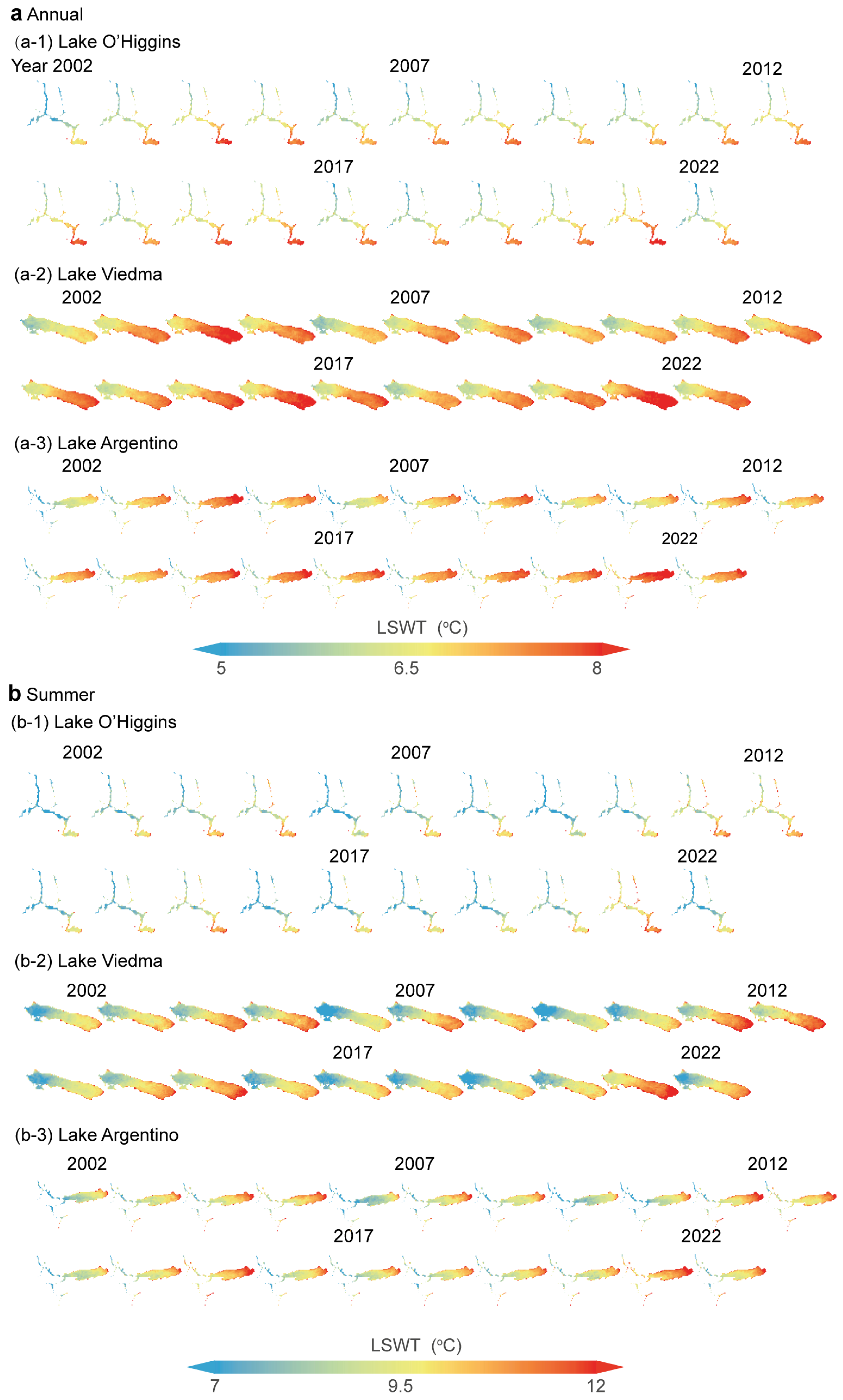
Analyze the LSWT spatial characteristics and trends of ice-contact lakes in relation to glaciers.
(iii)
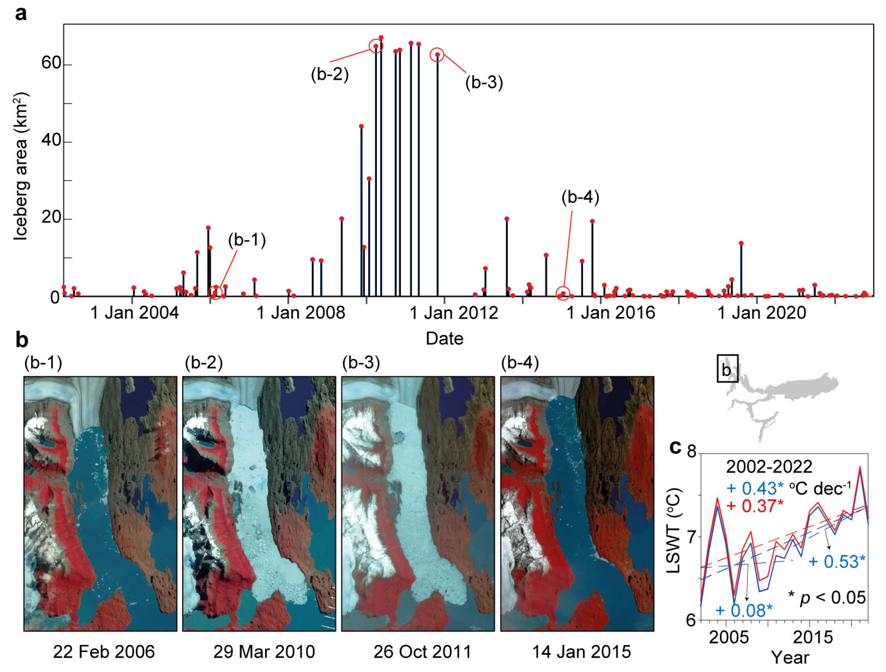
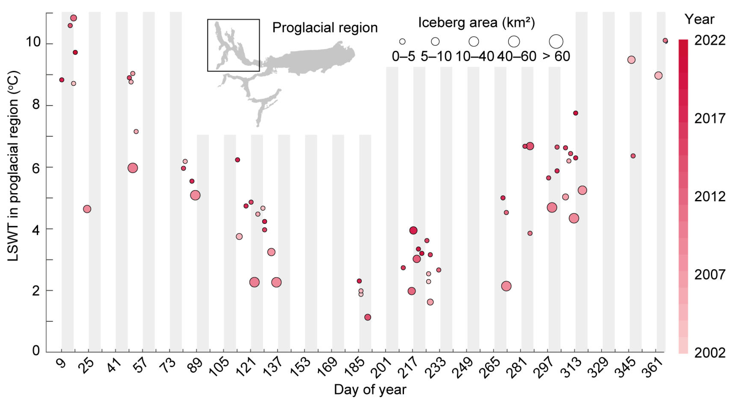
Analyze the cooling effect of calving events on ice-contact LSWT for Glacier Upsala, which experiences the most frequent calving events.
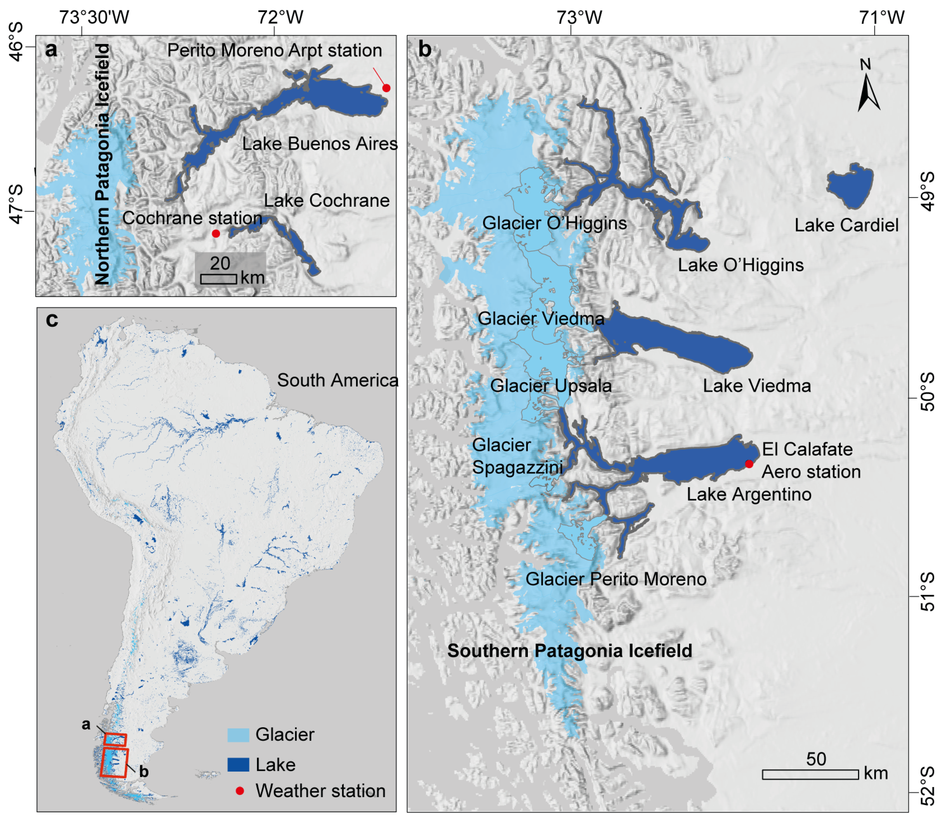
2. Study Area

Three ice-contact lakes (i.e., Lake Argentino, Lake Viedma, and Lake O’Higgins) in the Southern Patagonian Icefield were selected for LSWT analysis. Their considerable sizes, each surpassing 1000 km2, make them ideal targets for MODIS satellite observation. For better comparison, LSWT was also extracted from the three largest non-ice-contact lakes nearby (i.e., Lake Buenos Aires, Lake Cochrane, and Lake Cardiel) (Figure 1). All six of the selected lakes are located in the eastern flank of Andes, Patagonia. Patagonia features a climate shaped by its geographic position, the Andes Mountains, and the surrounding oceans. The region experiences stark contrasts in precipitation: the western side (Chile) receives abundant rainfall (2000–5000 mm annually) due to the influence of the westerlies, while the eastern side (Argentina) lies in the Andes rain shadow, with annual precipitation often below 200 mm, leading to arid or semi-arid conditions. Temperatures are generally low, with cold winters (below 0 °C) and cool summers (10–20 °C). Patagonia is also characterized by strong winds, particularly in the plains. Seasonal variations include relatively warmer, drier, and windier summers (December to February) and cooler, wetter winters (June to August) [22,23,24].

2.1. Ice-Contact Lakes

Lake Argentino, situated at an elevation of 179 m a.s.l. on the eastern side of the Southern Patagonia Icefield (latitude 50°15′ S, longitude 72°38′ W), covers an area of ~1494.2 km2 as of 2022, making it the world’s largest ice-contact lake [25]. The lake is long from east to west and narrow from north to south. The east and west ends span a straight-line distance of about 100 km, and the west end is connected to three glaciers in the Patagonia Icefield, Glacier Upsala, Glacier Perito Moreno and Glacier Spegazzini. The fjord connected to Glacier Upsala is more than 600 m in depth [26]. Glacier Upsala is also the fastest retreating glacier among the three glaciers, with its glacier terminus retreating by about 9 km since 1986. The annual air temperature of Lake Argentino is around 10 °C in summer and around −2 °C in winter. The wind speed on the lake surface is also high throughout the year, reaching about 14.2 m/s in summer and 6.8 m/s in winter, with prevailing westerly winds. Affected by strong winds, the entire lake has almost no ice-cover period [25]. Lake Viedma is situated in the middle of three ice-contact lakes in the Southern Patagonia Icefield, with geographical coordinates of 72°30′ W, 49°37′ S. As of 2022, the lake covers an area of ~1217.3 km2 at an elevation of 252 m a.s.l., extending approximately 80 km from east to west [27]. The western end of the lake is connected to the Glacier Viedma, the second largest glacier in the Southern Patagonia Icefield. In recent years, the retreating Glacier Viedma has led to lake expansion. In the vicinity of the glacier terminus, the depth of Lake Viedma exceeds 600 m [26]. Lake O’Higgins (also known as Lake San Martin) is located at the northernmost end of this group of ice-contact lakes, with coordinates of 72°41′ W, 48°51′ S. As of 2022, the lake covers an area of ~1049.9 km2 at an elevation of 252 m a.s.l., with an east–west extent of approximately 75 km. The western end of Lake O’Higgins is connected to the Glacier O’Higgins. Aerial photographs reveal that since 1896, the terminus of the O’Higgins Glacier has retreated by 19 km [28]. The deepest part of the lake, measured near the O’Higgins fjord, reaches nearly 800 m [26,29].

2.2. Non-Ice-Contact Lakes

Lake Buenos Aires (also known as Lake General Carrera) is a non-ice-contact glacier-fed lake located in the Northern Patagonia Icefield (72°30′ W, 46°39′ S). Covering an area of ~1858.0 km2 with a maximum depth of approximately 600 m and an elevation of 203 m a.s.l., and extending about 150 km from east to west, it ranks as the third largest lake in South America [30]. Lake Buenos Aires was last connected to the glacier between 11.7 and 15.5 kyr [31], but subsequently separated from the ice due to glacier retreat, while still receiving indirect glacier input through runoff. Lake Cochrane (71°58′ W, 47°18′ S), situated to the east of the Northern Patagonia Icefield and south of Lake Buenos Aires, is an elongated lake spanning approximately 60 km, with an area of ~338.4 km2 and an elevation of 152 m a.s.l., with glacier-fed meltwater input. Lake Cardiel, the southernmost non-ice-contact lake, is located at 71°11′ W, 48°56′ S, with an area of ~349.1 km2 and an elevation of 275 m a.s.l. The annual mean air temperature is ~7.5 °C, and the region, situated on the lee side of the Andes, is relatively arid, with an annual precipitation of ~210 mm [32].

3. Materials and Methods

3.1. Lake Area and Glacier Terminus Time Series

Extracting lake outlines is a prerequisite for generating LSWT products from MODIS imagery. The examined lakes include both ice-contact and non-ice-contact lakes. As the outlines of ice-contact lakes, particularly the part in contact with glaciers, exhibit greater variability, the extent of these lakes was delineated annually from 2002 to 2022 using manual interpretation of satellite imagery. Manual interpretation is considered a relatively accurate method for identifying lake boundaries [33]. Landsat Thematic Mapper (TM) (since 1982), Enhanced Thematic Mapper (ETM+) (since 1999), and Operational Land Imager (OLI) (since 2013) provide long-term, 30 m resolution land observations globally [34] and are widely used for identifying lake changes [35,36,37]. Landsat imagery was employed as a base map for delineating the boundaries of ice-contact lakes. Furthermore, while obtaining the lake boundaries, the terminal edges of their source glaciers that calve into the lakes were also extracted for a comprehensive analysis of lake and glacier dynamics. The extent of the three non-ice-contact lakes was derived from the global lake dataset HydroLAKES, which includes 1.4 million lakes worldwide [38].

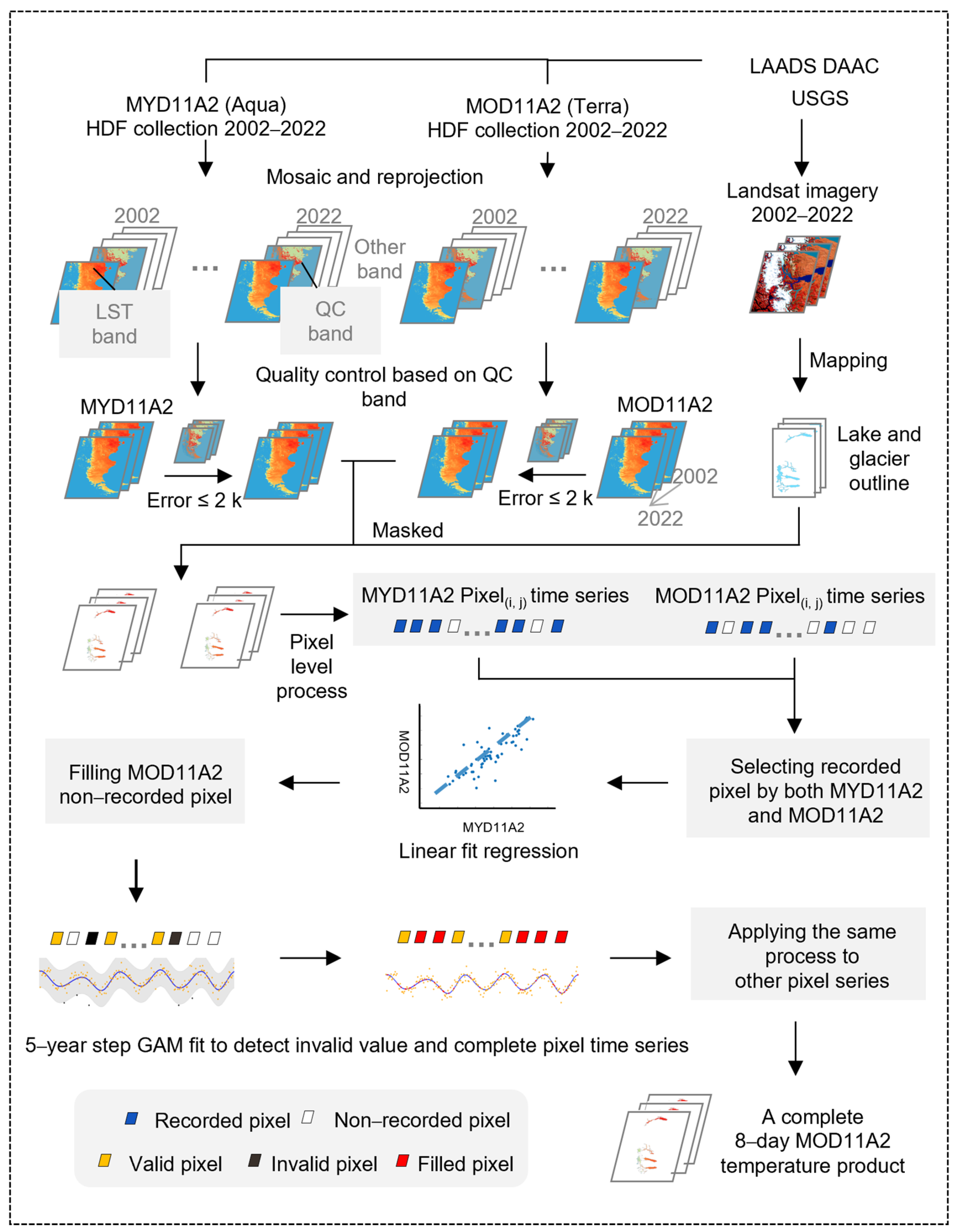
3.2. LSWT Derived from MODIS Data

MOD11A2 and MYD11A2, two land surface temperature products, were utilized in this study. These products were derived from the MODIS sensors aboard NASA’s Terra and Aqua satellites, respectively. Terra was launched on 18 December 1999, followed by Aqua on 4 May 2002. Terra and Aqua can acquire data over the same region twice daily, providing both day and night observations. Terra passes over a given location at approximately 10:30 a.m. and 10:30 p.m. local time, while Aqua passes at approximately 1:30 a.m. and 1:30 p.m. local time. These products have been widely used in studies of climate change [39], ecosystem [40] and drought monitoring [41]. The MODIS land surface temperature product is retrieved using the generalized split-window algorithm with a spatial resolution of 1 km. Both daily (MOD11A1 and MYD11A1) and 8-day composite (MOD11A2 and MYD11A2) data are available, with the latter being the 8-day average of the daily data. The products include day and night LSTs, quality control bands, observation time, viewing angle, and emissivity bands. These products are classified as Level 3, meaning they are geophysical products that have been processed over time and space, and are typically projected using a sinusoidal projection [42]. Considering the more complete data records in the 8-day composite data, this study adopted MOD11A2 and MYD11A2. To efficiently utilize the data, MOD11A2 was used as the base data and MYD11A2 was employed to fill the missing pixels in MOD11A2. Additionally, due to the greater thermal differences between the near and far ends of the ice-contact lake surface during the day caused by solar radiation, daytime, rather than nighttime, LSWT products were selected for analysis in this study.
The generation of LSWT products was based on MOD11A2 with the assistance of MYD11A2 (Figure 2). The MOD11A2 and MYD11A2 HDF data for six lakes from 2002 to 2022 were downloaded, mosaicked, and reprojected from sinusoidal to equal-area projection. After reprojection, the dataset was subjected to quality control using a quality assurance band to remove pixels with errors exceeding 2 K. The resulting dataset, containing both water and land, represents a preliminary quality-controlled MOD11A2 and MYD11A2 product. When extracting water body data for six lakes, the limited spatial resolution (1 km) leads to the inclusion of information from land in pixels near lake boundaries, contaminating the extracted LSWT. Additionally, the boundaries of ice-contact lakes exhibit rapid variations, further complicating the extraction process. Therefore, the extraction process needs to focus on two key aspects: accurately extracting pure water pixels and considering the temporal changes in lake boundaries and dynamically determining lake extents. For this purpose, by creating 1 km buffer zones inward from the vectorized lake boundaries at different time periods and converting them to raster masks, more accurate lake extents were produced that could assure only pure water pixels could be included, based on which water surface temperature for six lakes was separated from other objects.
The MOD11A2 surface temperature data for lakes still contains outliers and missing pixels that have not been fully addressed by the quality control bands. To obtain a complete and accurate dataset, further processing is required to remove these anomalies and fill in the gaps. The process involves a two-step approach. Firstly, gaps in the data are filled using the MYD11A2 dataset. Secondly, anomalies are removed and remaining missing values are filled using a Generalized Additive Model (GAM) function filter [43]. GAM provides a powerful tool for modeling complex relationships in data. It works by fitting smooth functions to each predictor variable, allowing for flexible modeling of non-linear relationships. Unlike traditional linear models, GAM does not require strict assumptions about the functional form of the relationship between the predictors and the response. By minimizing the residual sum of squares and penalizing model complexity, GAM offers a balance between model fitness and interpretability. This makes them particularly useful for addressing the curse of dimensionality in logistic regression and for modeling data with complex patterns. This model has been used to produce LSWT products [44]. These steps are carried out at the pixel level. Previous studies have successfully produced temperature products by combining MOD11A2 and MYD11A2 and have demonstrated promising validation [45]. For each row and column of lake pure pixels from 2002 to 2022, the subsequences where both MOD11A2 and MYD11A2 with observations were extracted. For these subsequences, a linear regression between MYD11A2 and MOD11A2 was performed to obtain a linear relationship:
TMOD11A2 = a × TMYD11A2 + b
Here, TMOD11A2 and TMYD11A2 represent the values of MOD11A2 and MYD11A2 in a pixel-level time series, respectively, and a and b represent the linear coefficient and constant term of the equation, respectively.
The missing values of MOD11A2 in the subsequence where MYD11A2 has observations were calculated based on the linear regression equation. Due to the unavailability of MYD11A2 data before July 2002, the filling step was not applicable to MOD11A2 data from that period. In this way, the LST product generated for 2002–2022 maximizes the utilization of the existing records from both Terra and Aqua.
After the initial filling of MOD11A2 using the MYD11A2-MOD11A2 linear relationship, GAM with a 5-year step was fitted to the pixel time series. Here, the standard deviation of residuals was calculated based on the 5-year-step GAM fitted values and corresponding MODIS LSWT observations:
σ s = i = 1 n s ( y i y ^ i ) 2 n s 1
where y i is the LSWT of the i-th satellite observation in a pixel time series, y ^ i is the corresponding fitted value from the GAM curve, and σ s is the standard deviation of residuals calculated from the observations within a 5-year step. Observations that deviated from the fitted values by more than three standard deviations of the residuals were classified as outliers and replaced with missing values. These newly created missing data points, together with any existing missing data, were then imputed using the corresponding fitted values from the GAM. This process produced a complete LSWT product for pure pixels within the six lakes, spanning the years 2002 to 2022.

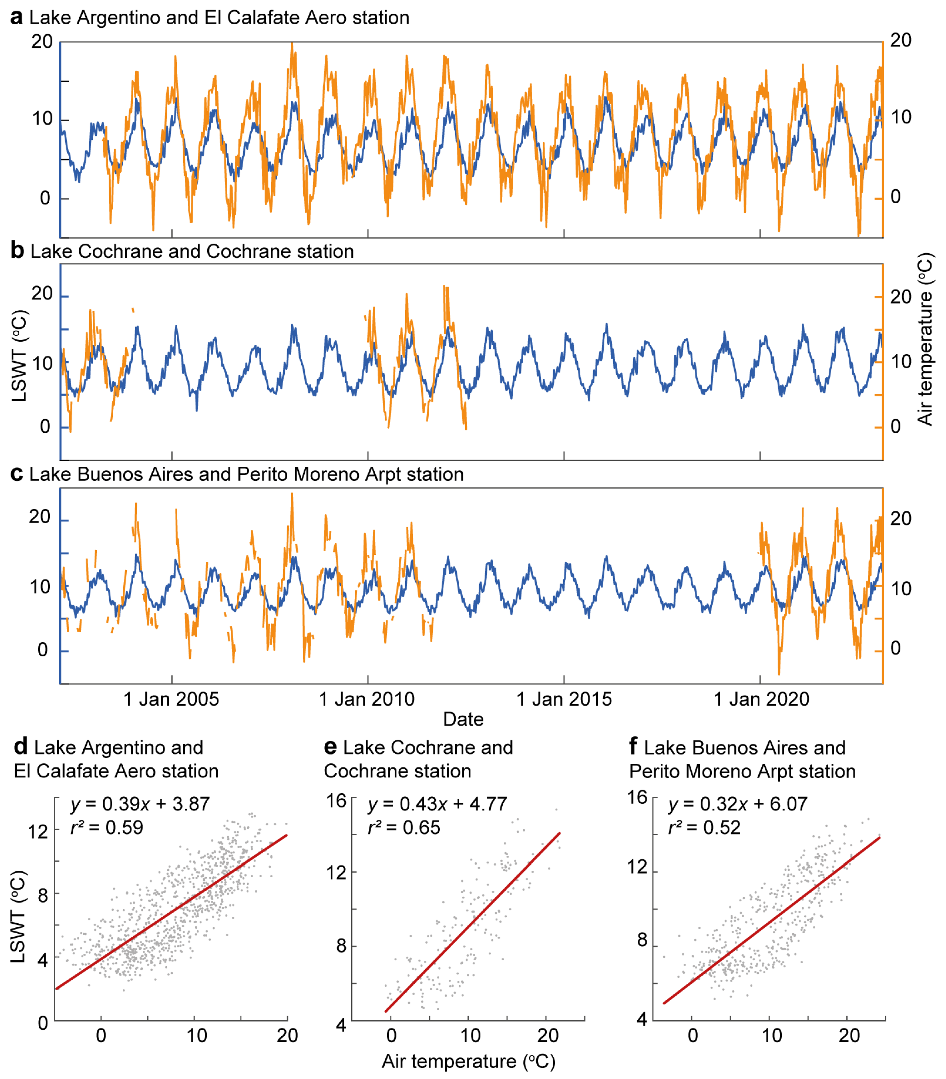
3.3. In Situ Lake Temperature, Air Temperature Data, and LSWT Validation

Among the six lakes, only the southernmost ice-contact lake, Lake Argentino, has in situ near water surface temperature observation data for validation [20]. The observation site (50.45° S, 73.02° W) is only 2 km from the front of Glacier Perito Moreno. The observation period is January 2009–December 2013, and the observation depth is 0–2 m [20]. When verified with the in situ data, MODIS LSWT is the monthly average LSWT of the entire range of Lake Argentino, showing good consistency with the in situ observations (Figure 3). In winter, the MODIS LSWT of the entire lake is lower than the in situ data, while in summer, the opposite is true (Figure 3a). The correlation r2 between MODIS LSWT and the in situ data reached 0.87 (Figure 3b), which shows the reliability of MODIS satellite observations. A comparison of MODIS LSWT and in situ observations of other lakes around the world also shows the accuracy of MODIS LSWT. For example, the correlation between field observations of lake surface temperature and MODIS observations reached r2 = 0.8 in Nam Co on the Tibetan Plateau [46] and r2 = 0.7 in Lake Malawi in Africa [47].
Given the scarcity of in situ lake surface temperature measurements, this study also utilized meteorological data from the NOAA Global Surface Summary of Day (GSOD) dataset for comparison with MODIS-derived LSWT. GSOD is compiled under the World Meteorological Organization; it is a comprehensive collection from over 9000 stations worldwide and is freely accessible for research, education, and other non-commercial purposes. GSOD data includes fields such as station name, code, date, and corresponding temperature, precipitation, visibility, and wind speed [48]. In this study, only the air temperature attribute TEMP was used, where the values represent the daily average air temperature in Fahrenheit. Only three meteorological stations with usable data were found near the six lakes (Figure 1): Perito Moreno Arpt station (71.0° W, 46.5° S, 429 m a.s.l.) near Lake Buenos Aires, Cochrane station (72.6° W, 47.2° S, 196 m a.s.l.) near Lake Cochrane, and El Calafate Aero station (72.1° W, 50.3° S, 199 m a.s.l.) near Lake Argentino. Therefore, this study only validated the LSWT of these three lakes. Daily air temperatures were averaged over 8-day periods to correspond with the temporal resolution of the MODIS 8-day LSWT product. If there were fewer than 5 air temperature records within an 8-day period, the data were discarded; otherwise, the average was calculated. The resulting 8-day series for the three meteorological stations and the corresponding 8-day LSWT series for the three lakes were visually displayed and plotted as scatterplots.
Among three stations, the El Calafate Aero station, located southeast of Lake Argentino, had the most complete and continuous temperature record over the 20 years (Figure 4a). The other two stations exhibit obvious data gaps, especially the Cochrane station (Figure 4b). For downscaled eight-day air temperature records, the valid record ratios of the three meteorological stations El Carafate Aero station, Cochrane station, and Perito Moreno Arpt station in 2002–2022 were 94%, 19%, and 45%, respectively. The time series from the meteorological stations show that air temperature has a larger amplitude of variation compared to LSWT due to the higher specific heat capacity of water. Air temperature is generally higher than LSWT in summer and lower in winter. Overall, LSWT demonstrates a consistent response to air temperature variations in both long-term changes and short-term fluctuations. The scatter plots reveal a correlation between LSWT and air temperature. The r2 values for Lake Argentino, Lake Cochrane, and Lake Buenos Aires are 0.59, 0.65, and 0.52, respectively, indicating a relatively good fit between the two variables (Figure 4d–f). The different correlations between the air temperature records at different meteorological stations and MODIS LSWT are possibly not only related to the differences in the amount of meteorological data at each station but also to the size of the lake’s heat capacity and the terrain around the lake.

3.4. Calving Events of Lake Argentino

Lake Argentino is unique due to the significant retreat and more frequent, larger-scale calving events of Glacier Upsala, which calves into the lake Compared to other glaciers in contact with the three lakes, these changes have led to a greater impact on the LSWT of the entire lake, particularly in the ice-proximal region [26]. This study utilizes accessible, cloud-free Landsat imagery to map iceberg coverage on Lake Argentino from 2002 to 2022. The characteristics of calving events of various scales over the past two decades and their impact on the LSWT of the ice-proximal region were investigated. Here, ice-proximal region was defined as the arm of the lake from the terminus connected to Glacier Upsala, extending to one-third of the lake’s east–west length.

4. Results

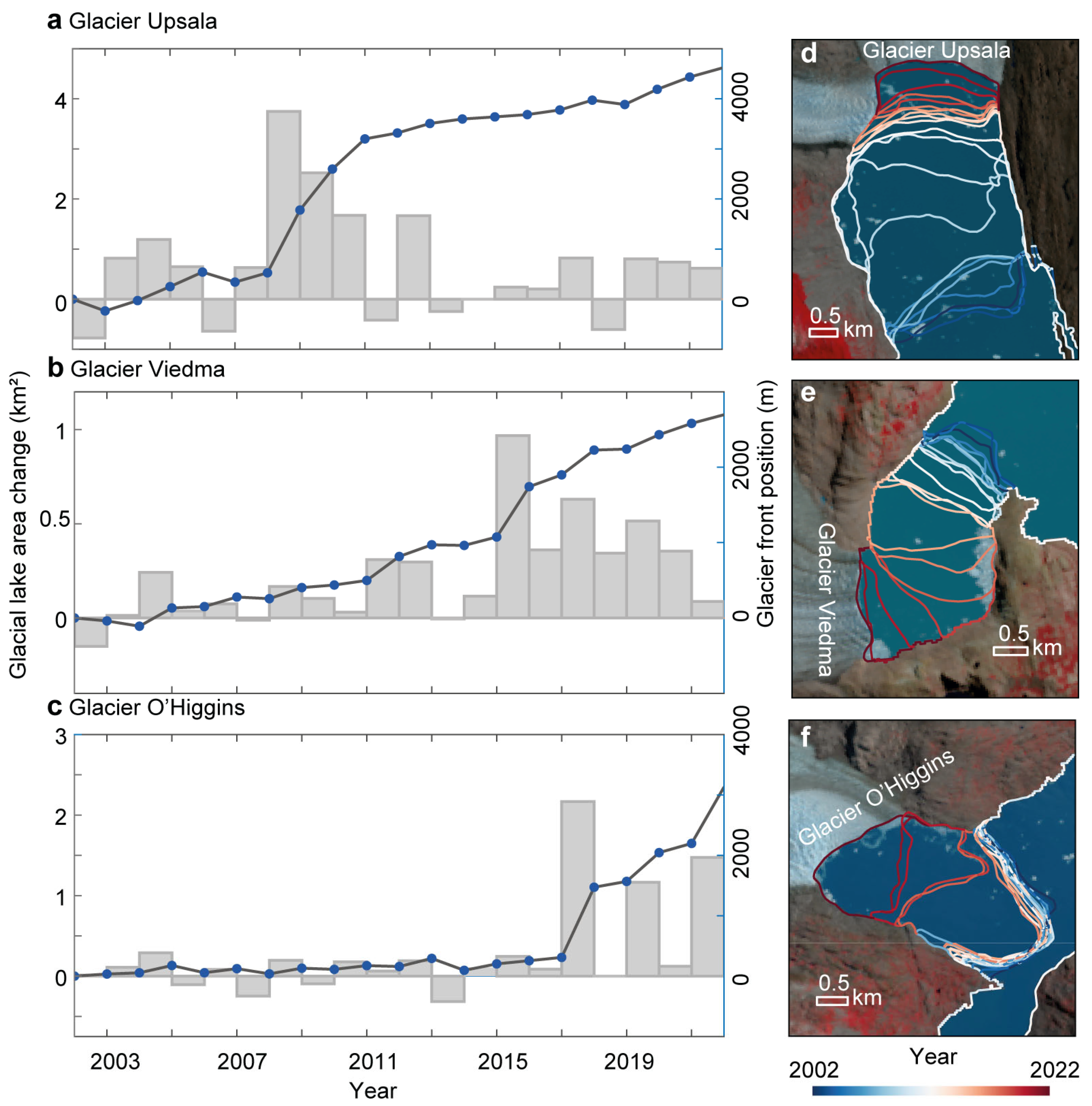
4.1. Ice-Contact Lake and Glacier Dynamics

All three ice-contact lakes exhibited an expanding trend in area. From 2002 to 2022, Lake Argentino expanded from about 1480.5 to 1494.2 km2, with an increase of 13.7 km2, the largest expansion among the three lakes. Lake Viedma expanded from 1212.9 to 1217.3 km2, with an increase of 4.4 km2, and Lake O’Higgins expanded from 1044.2 to 1049.9 km2, with an increase of 5.7 km2. The changes in different lakes also varied across different years and showed a correlation with changes in the terminus positions (at the glacier centerline) of their mother glaciers (Figure 5a–c). The changes in Lake Argentino were primarily driven by changes in the terminus of Glacier Upsala. In most years, the position of Glacier Upsala remained relatively stable, and the area of Lake Argentino correspondingly changed by less than 1 km2. However, between 2008 and 2010, the terminus of Glacier Upsala retreated 2.1 km up-glacier, with a 6.3 km2 area expansion of Lake Argentino. Lake Viedma and Lake O’Higgins showed marked expansion only in 2015–2016 and 2017–2018, expanding by 0.9 and 2.2 km2, respectively, coinciding with the years of maximum retreat of their glacier termini (0.7 and 1.1 km, respectively).

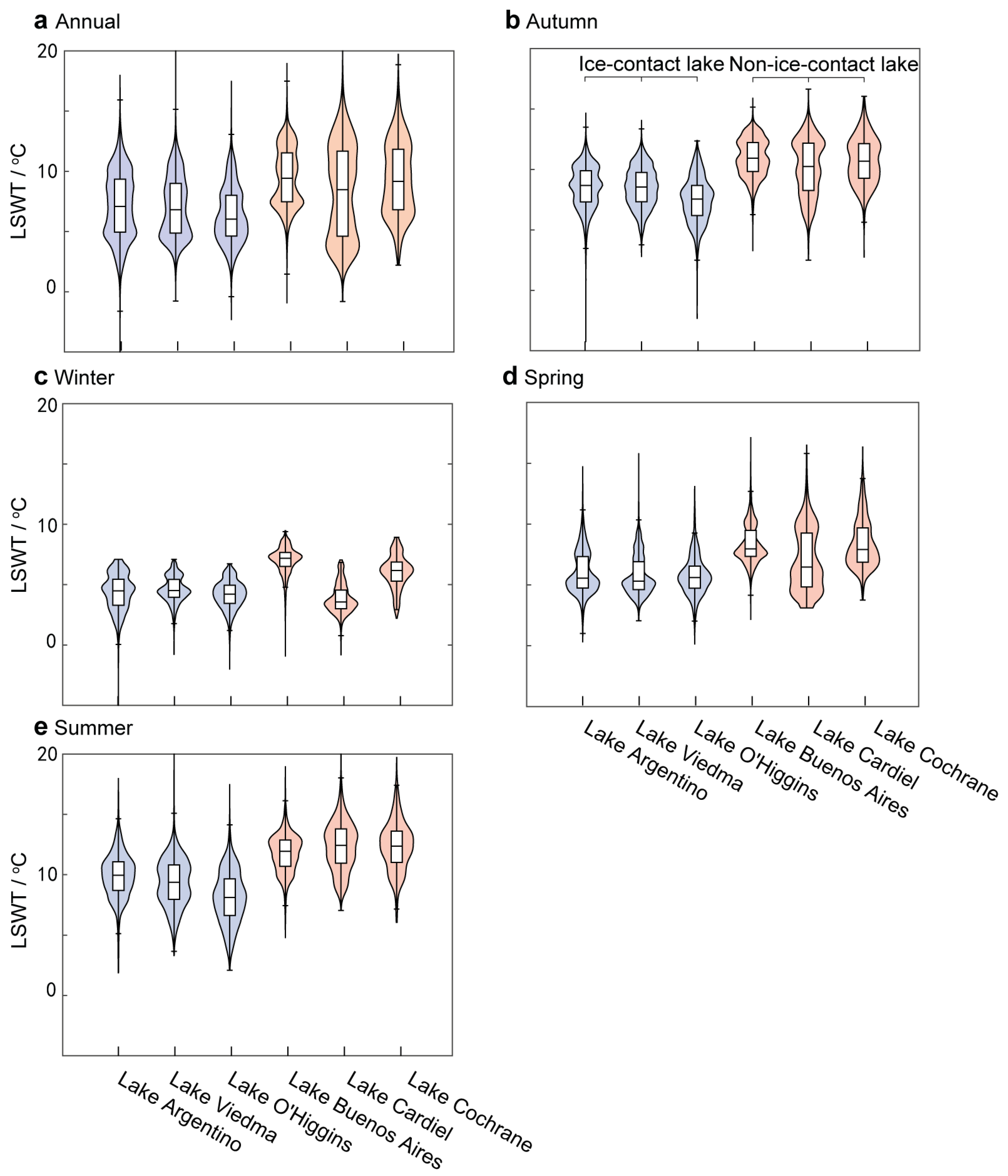
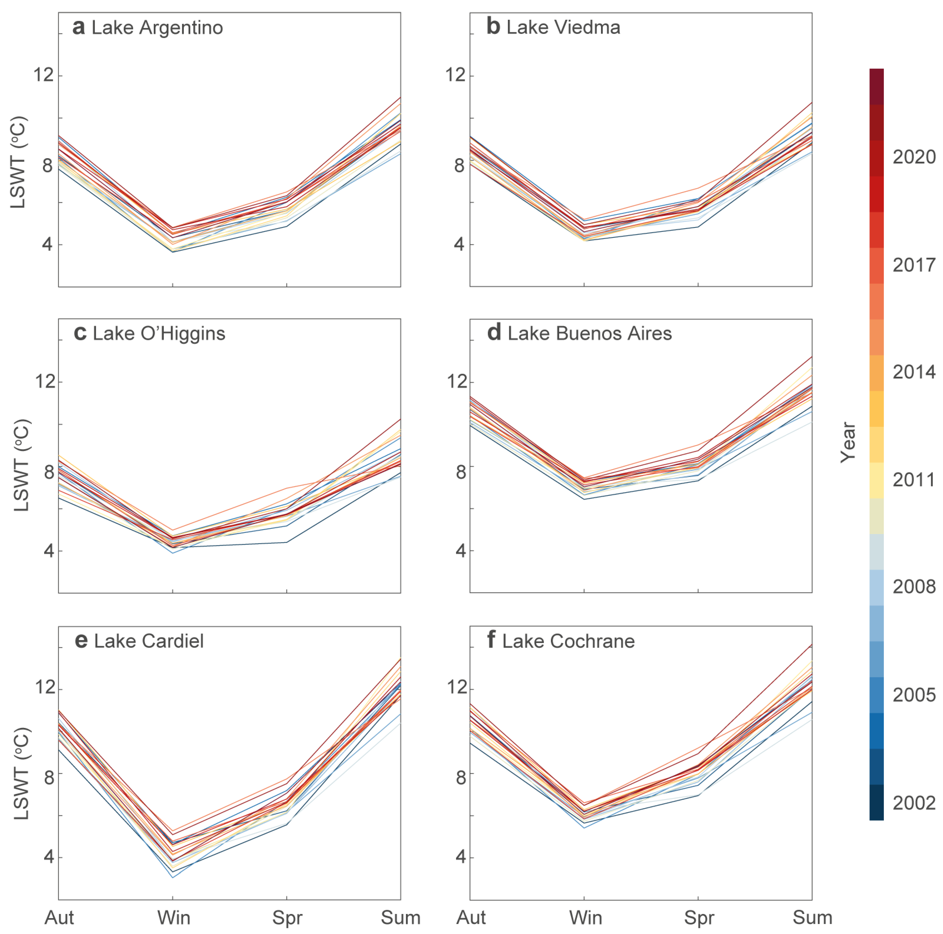
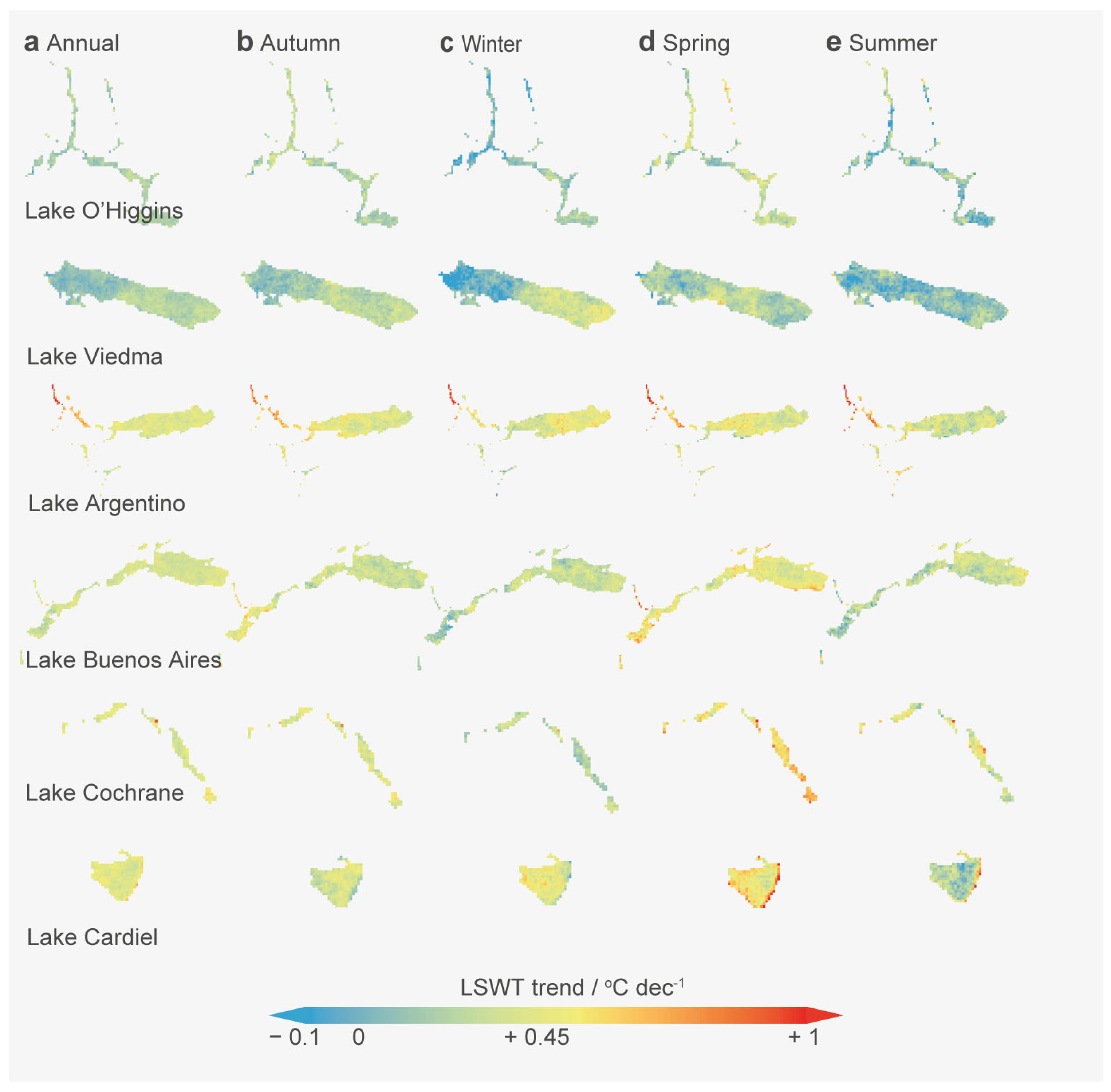
4.2. Annual and Seasonal LSWT Pattern

As the latest year of this study, 2022 is used as an example to illustrate the annual, seasonal, and spatial distribution characteristics of lake LSWT. On an annual scale, the surface temperature of ice-contact lakes is generally lower than that of non-ice-contact lakes (Figure 6a). In 2022, Lake Argentino had the highest average LSWT at 7.2 °C, followed by Lake Viedma (7.0 °C) and Lake O’Higgins (6.4 °C). Even Lake Cardiel, the coldest of the non-ice-contact lakes with a mean LSWT of 8.3 °C, exhibited higher than the three ice-contact lakes. Beyond latitudinal factors, the cooling effect of glaciers is likely a contributing factor to this phenomenon.
Seasonally, the average LSWT of the three ice-contact lakes was closest to each other during spring and winter in 2022. In summer and autumn, Lake Argentino and Lake Viedma exhibited similar average LSWT, while Lake O’Higgins was relatively lower. The average LSWT of all ice-contact lakes in autumn, winter, spring, and summer were 8.3, 4.6, 5.4, and 9 °C, respectively. LSWT in autumn was higher than that of spring, while the difference between spring and winter LSWT was relatively smaller. The LSWT difference between ice-contact and non-ice-contact lakes was most pronounced in summer. Additionally, the standard deviation of ice-contact LSWT was largest in summer compared to other seasons, highlighting the influence of glacier contact (Table 1). From the seasonal average LSWT (Figure 7), both ice-contact and non-ice-contact lakes exhibit a consistent cycle of LSWT with summer > autumn > spring > winter. The LSWT of non-ice-contact lakes is lower than that of ice-contact lakes in all seasons, except for Lake Cardiel in winter. The cooling effect of glacial contact leads to a general LSWT difference between non-ice-contact and ice-contact lakes, while the smaller heat capacity caused by the shallower basin of Lake Cardiel (average depth of 18 m according to HydroLAKES dataset, the shallowest among all lakes) makes the LSWT more sensitive to cold winter than other non-ice-contact lakes. At the same time, the latitude of Lake Cardiel is the highest among non-ice-contact lakes, which leads to significantly lower LSWT in winter, even close to the winter LSWT of ice-contact lakes. The average LSWT of all lakes in each season was generally lower in the early years (2002–2022) compared to later years, which is likely related to the ongoing climate warming trend (Figure 7).
Spatial heterogeneity of LSWT in ice-contact lakes from 2002 to 2022, both interannually and seasonally (only the summer pattern was displayed due to its obvious difference), was illustrated (Figure 8). The LSWT of ice-contact lakes exhibits a pattern of colder temperatures near the glacier terminus and warmer temperatures further away. This temperature difference is most pronounced in summer and also varies between years, potentially related to annual mean air temperature, glacial meltwater input, and the frequency and magnitude of calving events.

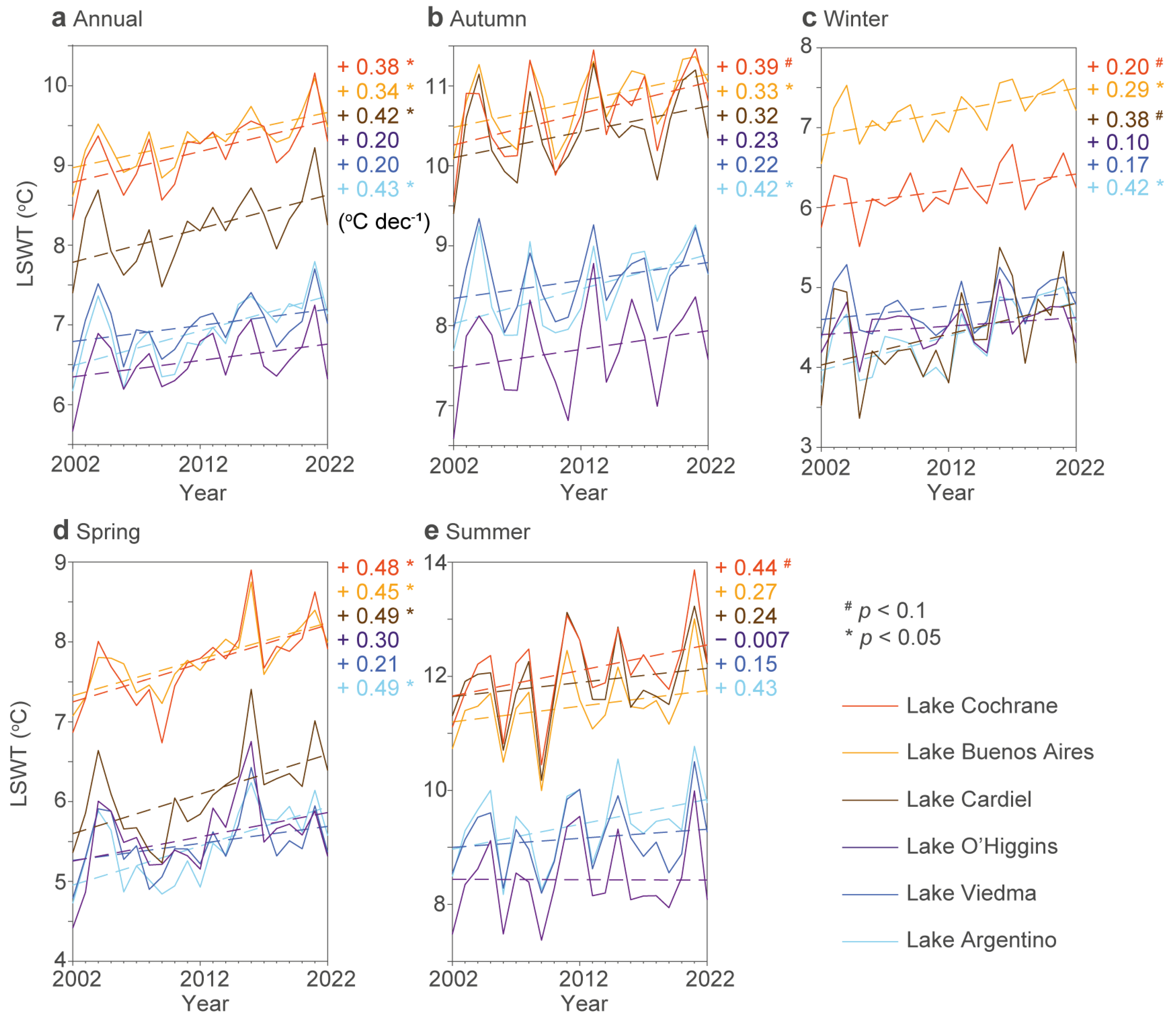
4.3. LSWT Trend Between 2002 and 2022

Over the past two decades, the LSWT trends of ice-contact and non-ice-contact lakes have shown distinct variations. On the annual scale, all three non-ice-contact lakes exhibited significant (p < 0.05) warming trends, with warming rates of +0.38 °C dec−1 for Lake Cochrane, +0.42 °C dec−1 for Lake Cardiel, and +0.34 °C dec−1 for Lake Buenos Aires (Figure 9a). In contrast, two of the three ice-contact lakes, Lake Viedma and Lake O’Higgins, did not show significant warming trends (p > 0.1). However, Lake Argentino, as an ice-contact lake, exhibited an anomalous behavior: not only did it show a significant warming trend, but its rate was higher than all non-ice-contact lakes at +0.43 °C dec−1. Spatially, the LSWT trends of different parts of ice-contact lakes, compared to non-ice-contact lakes, were markedly related to their distance from the glacier terminus. For Lake Viedma and Lake O’Higgins, the annual warming rate was slower near the glacial terminus and faster farther away, reflecting the spatial variability in the inhibitory effect of glaciers on lake warming. While Lake Argentino showed a spatial pattern distinctly different from the other two ice-contact lakes: the near-glacier (Glacier Upsala) end warmed faster, while the far-glacier end warmed more slowly. Particularly, in the ice-proximal fjord within 13 km of Glacier Upsala’s terminus (in 2002), the LSWT warming rate reached around 1 °C dec−1, approximately twice that of the far-glacier end of Lake Argentino, which was around 0.4 °C dec−1 (Figure 10).
Seasonally, over the past two decades, neither Lake Viedma nor Lake O’Higgins showed significant warming trends in any season. In contrast, Lake Argentino exhibited significant warming trends in autumn, winter, and spring, with rates of +0.42, +0.42, and +0.49 °C dec−1, respectively. The fastest warming rate for Lake Argentino occurred in spring, which is consistent with the pattern observed in non-ice-contact lakes. Except for Lake Buenos Aires, no significant warming trends were observed in summer for any of the lakes.

5. Discussion

As observed in regions like Greenland [49] and Alaska [37], the numerous ice-contact lakes of the Patagonia Icefield have expanded significantly in recent decades due to glacier retreat, contributing substantially to the glacial lake volume [36,50]. Consequently, the mechanical and thermal interactions [19,51] between glaciers and these lakes have garnered increasing research interest. Within the study of these thermal interactions, data on the vertical and surface thermal conditions of ice-contact lakes are fundamental. While vertical thermal regimes of ice-contact lakes in Patagonia have been analyzed for Lake Argentino [20], Lake Viedma [18], and Lake Grey [19], observations of surface thermal regime are limited to scattered single points [20]. This scarcity of comprehensive surface LSWT data, particularly long-term, whole-lake observations, is a common issue shared with other regions globally, including Scandinavia [14], North America [52], and the Himalaya [17]. In this context, this study, using satellite remote sensing observations, generated an LSWT product revealing the surface thermal regimes of the world’s three largest ice-contact lakes in the Patagonian region from 2002 to 2022, with a temporal resolution of 8-day and a spatial resolution of 1 km. These demonstrate the spatial distribution and long-term trends of their LSWT.

5.1. Glaciers’ and Other Possible Factors’ Impact on Ice-Contact LSWT

The average LSWT of the three ice-contact lakes in summer is 9 °C, which is close to the average LSWT of 8.9 °C measured in summer for ice-contact lakes in Arctic Sweden [14], the maximum LSWT of 10 °C measured using thermistors in ice-contact lakes in New Zealand [53], and the 10 °C measured in Nepal [17]. The spatial cold–warm difference between the near-glacier and far-glacier ends is also consistent with that observed in ice-contact lakes in Arctic Sweden [14] and New Zealand [53], i.e., colder near the glacier and warmer farther away, reflecting the cooling effect of glacier contact. Notably, the three ice-contact lakes in this study are significantly larger in area than those in Arctic Sweden and New Zealand. The fact that such large lakes still exhibit LSWT differences between the near-glacier and far-glacier ends may also be related to the prevailing westerly winds in the region [25]. Strong winds drive surface water currents, continuously transporting newly generated meltwater from the glacier terminus towards areas further away, thus extending the influence of glacier contact cooling. Seasonally, this difference is most pronounced in the three very large ice-contact lakes during summer (Figure 8) and the LSWT standard deviations in the temperature distribution are also broader compared to other seasons (Table 1). This reflects the seasonal variation in the glacier contact cooling effect. As air temperature increases in summer, glacial meltwater input also increases. Consequently, the LSWT near the glacier terminus of ice-contact lakes is significantly influenced by the increased glacier meltwater supply, while the far end is less influenced by glacier meltwater and more affected by enhanced solar radiation. This results in a wider distribution of LSWT compared to other seasons, leading to a more pronounced pattern of colder near-glacier end water and warmer far-glacier water in summer. Additionally, stronger winds in summer compared to other seasons further amplify this seasonal difference [54]. In most years from 2002 to 2022, the LSWT of Lake Argentino and Lake Viedma was closer, while for Lake O’Higgins it was lower (Figure 9 and Figure 10 and Table 1). In terms of seasons, this phenomenon is obvious in summer and autumn, but not in winter and spring. These lakes have higher air temperatures in summer and autumn, which are the main seasons for glacier melting. At the same time, during the period 2000–2019, the annual frontal ablation at the end of the Glacier O’Higgins, which is in contact with Lake O’Higgins, was higher than that of the parent glaciers of the other two ice-contact lakes [55]. The greater meltwater supply may have caused the annual and seasonal differences between Lake O’Higgins and Lake Argentino and Lake Viedma. In addition, in terms of the terrain around the lakes and their own shapes, most parts of Lake Argentino and Lake Viedma are located on a wider plain, and the lake presents a wider surface, while Lake O’Higgins is located in a deep mountain canyon with a long and narrow shape. The relatively narrow lake surface limits the total amount of solar radiation absorbed, which may also result in lower LSWT. According to the HydroLAKES dataset, Lake O’Higgins has an average depth of 68 m, which is shallower than both Lake Argentino (166 m) and Lake Viedma (100 m). This shallower depth results in a lower heat capacity for Lake O’Higgins, making it more sensitive to glacier meltwater discharge and cold Spring and Winter, thus also making it a possible factor in the observed LSWT differences.
Runoff also affects the LSWT of ice-contact lakes. The La Leona River connects Lake Viedma and Lake Argentino and supplies water from Lake Viedma to Lake Argentino, which is one of its sources of water input. The summer flow of the La Leona River (~527 m3 s−1) is much greater than the winter flow (~83 m3 s−1), which is consistent with the seasonal changes in glacial meltwater [25]. It also carries a large amount of sediment into Lake Argentino. The suspended particles entering Lake Argentino enhance light absorption and reduce the depth of light penetration, which may increase the LSWT near the entrance to the lake. However, Lake Argentino is large in area and has strong thermal inertia of the water body. Therefore, sediment input may mainly affect the area entering the lake and have little effect on the LSWT of the entire lake.
Regarding the 20-year LSWT change trends in the ice-contact lakes, both Lake Viedma and Lake O’Higgins exhibited insignificant LSWT change trends on both annual and seasonal scales (Figure 9). Spatially, the part closer to the glaciers in these two lakes warmed more slowly than the parts further away (Figure 10), demonstrating the inhibiting effect of glaciers on the warming of ice-contact lakes. Glacial meltwater replenishes the lakes with cold meltwater, offsetting the warming effect of the lakes under climate warming. However, Lake Argentino was an exception, showing a significant warming trend on annual and some seasonal scales, even exceeding the warming rate of non-ice-contact lakes at times (Figure 9). Spatially, Lake Argentino warmed fastest near the glacier terminus, with a warming rate twice that of the far end, which is contrary to the other two ice-contact lakes. This was likely attributed to a major calving event (Figure 11). Based on the interpretation of the iceberg area sequence of Lake Argentino from available Landsat imagery between 2002 and 2022, several large calving events occurred from late 2009 to early 2010, resulting in a sharp retreat of the glacier area and a marked increase in iceberg accumulation area, exceeding 64 km2 of accumulation on 29 March 2010 (Figure 10a), and lasting until 26 October 2011, a duration of one and a half years. During this period, icebergs filled the entire fjord from the glacier terminus to 13 km into the lake (Figure 11b). Subsequently, the iceberg accumulation area gradually decreased, and the accumulated icebergs gradually melted. Segmented analyses of the annual LSWT trend of Lake Argentino for 2002–2012 and 2012–2022 showed that the lake warming was mainly driven by the trend in the latter ten years (Figure 11c), which corresponds to the period after the large-scale iceberg accumulation event. Furthermore, trend analysis of the remaining area of Lake Argentino after removing the fjord filled with icebergs over the past 20 years showed a warming rate of 0.37 °C dec−1 (Figure 11a), which is lower than the warming rate of the entire lake and also lower than the warming rate of non-ice-contact lakes.
Due to the large accumulation area, long duration, and dense packing of icebergs during this major calving event, the temperature records captured by MODIS imagery during this period were more representative of ice surface temperature than the LSWT, leading to an underestimation of LSWT in this area, even though the LSWT in this area was already relatively low due to the large input of cold meltwater from the iceberg melting process. Meanwhile, the prevailing westerly winds continuously transported meltwater from the large accumulation of melting icebergs to other parts of the lake, disrupting the meltwater input balance from the glacier in other periods, causing some areas to experience cooling followed by a return to a normal level. Furthermore, similar to the Arctic amplification effect [56,57], the icebergs, with an accumulation area of about 64 km2, had a high albedo and thus absorbed less solar radiation. They gradually melted after October 2011 and the high-albedo accumulated icebergs were replaced by low-albedo lake water, resulting in a significant increase in solar radiation absorption. This could likely also be a reason for the significant warming rate of Lake Argentino, especially in terms of iceberg accumulation.
From the perspective of global lakes, under the background of global warming, heatwave events in the LSWT are expected to continue to intensify by the end of this century. For the high greenhouse gas emission scenario (Representative Concentration Pathway (RCP) 8.5), the average intensity of lake heatwaves defined in the historical period (1970 to 1999) will increase from 3.7 ± 0.1 to 5.4 ± 0.8 °C, and their average duration will increase significantly from 7.7 ± 0.4 to 95.5 ± 35.3 days. In the low-greenhouse-gas-emission RCP 2.6 scenario, the intensity and duration of heatwaves will increase to 4.0 ± 0.2 °C and 27.0 ± 7.6 days, respectively [58]. As a special category that is significantly affected by glacier contact, whether ice-contact lakes have historical extreme heatwave events, to what extent their extreme heatwave events will be suppressed by glaciers, how they will develop in the future, and what impact they will have on glacier dynamics. These are all scientific issues worthy of attention.

5.2. Calving Events’ Impact on Ice-Contact LSWT

Besides the direct cooling effect of glacier contact on ice-contact LSWT, calving events also cause fluctuations in LSWT. Given the rapid retreat, relatively frequent calving events, and occurrence of large-scale calving events of Glacier Upsala [59,60], which terminates in Lake Argentino, in recent decades, this study focuses on this glacier. Based on available Landsat imagery from 2002 to 2022, iceberg areas at different times were collected to characterize the timing and scale of calving events. In addition to exploring the impact of calving events on the warming trend of Lake Argentino (see Section 5.1), the study also analyzed the cooling effect of calving event scale on the ice-proximal part of Lake Argentino.
From iceberg area mapping in the past 20 years in front of Glacier Upsala in Lake Argentino (Figure 11a), it can be seen that due to local weather conditions, a total of 118 iceberg area records were collected over 20 years from clean images, with an average of about 6 records per year. All iceberg areas were greater than 0, with the smallest being 0.01 km2 and the largest being 67 km2 on 16 May 2010. There were 96 dates with iceberg areas of 0–5 km2, accounting for about 80% of the total records; 6 dates with 5–10 km2, accounting for 5%; 10 dates with 10–40 km2, accounting for about 9%; only 1 record with 40–60 km2 on 13 November 2009; and 7 records with iceberg areas greater than 60 km2. This shows that calving events at Glacier Upsala are relatively frequent, but mostly small-scale. The seven records greater than 60 km2 are related to the large-scale calving event mentioned in Section 5.1 that occurred in early 2010 at Glacier Upsala, resulting in a large-area, long-term iceberg accumulation event, which has been rare in the past 20 years.
This study collects data on the iceberg areas in different years but on similar day of year (falling in the same MODIS 8-day interval), obtains the average LSWT of the next three consecutive MODIS 8-day records in the Lake Argentino ice-proximal area, and explores the cooling of LSWT caused by different scales of calving events (Figure 12). The results show that calving events of various scales lead to a short-term decrease in LSWT in the ice-proximal area, and the larger the calving scale, i.e., the larger the generated iceberg area, the more marked the short-term cooling effect. For example, on 20 February 2011 (corresponding to a day of year 49 of the MODIS 8-day product), 65.7 km2 of iceberg accumulation was captured, and the corresponding LSWT of the ice-proximal part within the following 24 days was only 5.9 °C, which is lower than the LSWT of other close dates in other years (19 February 2005, 22 February 2006, 20 February 2008, and 18 February 2016) with smaller iceberg areas (all <5 km2), which had LSWTs of 8.7, 7.1, 9.0, and 8.8 °C, respectively.
Consistent with the effect of calving events on LSWT, the cooling effect of icebergs on ice-contact lakes in North America near Bridge Glacier has also been demonstrated, showing a warming trend in lake surface temperature after the iceberg area has peaked [21]. A study on Thulagi Lake in the Himalaya also observed a sharp drop in surface temperature after a calving event in 2017. This study also established an empirical formula for iceberg area–volume using drones to calculate the heat required for iceberg melting, thereby more accurately determining the impact of calving events on the surface thermal regime of ice-contact lakes [17].

5.3. Ice-Contact LSWT Impact on Glacier

Compared with the vertical thermal structure of ice-contact lakes, which have different effects on glacier morphology due to differential melting at different depths [18], the surface thermal conditions of ice-contact lakes mainly affect the melting rate of glaciers at the waterline, which in turn produces thermal notch erosion, leading to intensive calving events. After that, the glacier morphology stabilizes again and the frequency of calving events decreases [16]. At the same time, according to the conclusions of this study and other studies, the icebergs produced by calving events cause the ice-contact lake to cool down, which will also inhibit thermal notch erosion. In the future, the study of LSWT and thermal notch erosion in ice-contact lakes needs to be further strengthened by combining field measurements and satellite remote sensing observations. Thermal erosion notches usually extend into the interior of the glacier and are hidden under the end of the glacier. Quantifying their erosion rate notches not only faces certain safety risks but is also not conducive to accurate and efficient measurement. Field cameras may play a role in solving the quantification problem. This has been used in an ice-dammed lake in Greenland to observe the seasonality of calving events [61]. For the extraction of LSWT of glacial lakes, although the temporal resolution of MODIS satellites is relatively high, considering that the area of glacial lakes is generally small, the thermal infrared bands of sensors with higher spatial resolution such as Landsat and ASTER can be used. As the most accurate means of observation, thermometers can be placed, especially near the end of glaciers, to comprehensively observe LSWT, provide a basis for verification of satellite observations, and better understand the relationship between LSWT and thermal undercutting. In addition, similarly to the study of the interaction between tidewater glaciers and fjords [62], the development and application of physical models suitable for glacial lakes will also play a positive role in the simulation of glacier–lake thermal interactions.

6. Conclusions

Against the backdrop of climate warming, the Patagonian Icefield has experienced significant glacial lake expansion in recent decades, with ice-contact lakes contributing prominently to this trend. The LSWT of ice-contact lakes plays a critical role in influencing glacier melting at the waterline. However, most observations of LSWT in ice-contact lakes rely on short-term, field-based point measurements. The typically small size of ice-contact lakes further limits the application of thermal infrared bands in satellite remote sensing, hindering a comprehensive understanding of their surface thermal regime. This study utilizes MODIS land surface temperature products to analyze the three largest ice-contact lakes in the Patagonia Icefield—Lake Argentino, Lake Viedma, and Lake O’Higgins—each exceeding 1000 km2. Complete 8-day LSWT records from 2002 to 2022 were obtained, providing insight into the spatial and temporal variations in LSWT and their relationship with glacier dynamics.
On an annual scale, the mean LSWTs of Lake Argentino, Lake Viedma, and Lake O’Higgins in 2022 were lower than those of the three largest nearby non-ice-contact lakes. In summer, ice-contact lakes exhibited broader temperature distributions compared to other seasons. Spatially, LSWT was lower near glacier termini, with the temperature gradient between glacier-proximal and glacier-distal regions being most pronounced in summer. This pattern reflects the cooling of glacier contact and its seasonal variability. Over the past two decades, Lake Viedma and Lake O’Higgins exhibited non-significant LSWT trends, contrasting with the significant warming observed in non-ice-contact lakes. This highlights the suppressive effect of glacier contact on LSWT warming. Conversely, Lake Argentino showed a significant warming trend (+0.43 °C dec−1, p < 0.05), with the fastest warming occurring in ice-proximal areas. This anomaly is hypothesized to be linked to a prolonged iceberg accumulation event from 2010 to 2011, lasting over 18 months. Frequent calving events from Glacier Upsala over the past two decades further influenced short-term LSWT cooling in ice-proximal regions of Lake Argentino, with larger calving events inducing more pronounced cooling within at least 24 days. This study elucidates the spatial and temporal surface thermal regime of three major ice-contact lakes, emphasizing the importance of integrating field observations and remote sensing to further explore LSWT dynamics and their implications for glacier frontal ablation.

Author Contributions

Conceptualization, S.Z. and G.Z.; Methodology, S.Z.; Writing—original draft, S.Z.; Writing—review and editing, H.S. and J.C.; Supervision, G.Z. All authors have read and agreed to the published version of the manuscript.

Funding

This research received no external funding.

Data Availability Statement

MODIS imagery was downloaded from https://search.earthdata.nasa.gov/ (last access on 8 November 2024). The Landsat imagery was downloaded from https://glovis.usgs.gov/ (last access on 21 November 2024).

Acknowledgments

The authors would like to thank F.X. for providing suggestions on the figure designments and the reviewers for their valuable comments.

Conflicts of Interest

The authors declare no conflicts of interest.

References

  1. Abdel Jaber, W.; Rott, H.; Floricioiu, D.; Wuite, J.; Miranda, N. Heterogeneous Spatial and Temporal Pattern of Surface Elevation Change and Mass Balance of the Patagonian Ice Fields between 2000 and 2016. Cryosphere 2019, 13, 2511–2535. [Google Scholar] [CrossRef]
  2. Davies, B.J.; Glasser, N.F. Accelerating Shrinkage of Patagonian Glaciers from the Little Ice Age (~AD 1870) to 2011. J. Glaciol. 2012, 58, 1063–1084. [Google Scholar] [CrossRef]
  3. Hugonnet, R.; McNabb, R.; Berthier, E.; Menounos, B.; Nuth, C.; Girod, L.; Farinotti, D.; Huss, M.; Dussaillant, I.; Brun, F.; et al. Accelerated Global Glacier Mass Loss in the Early Twenty-First Century. Nature 2021, 592, 726–731. [Google Scholar] [CrossRef] [PubMed]
  4. Aniya, M.; Sato, H.; Naruse, R.; Skvarca, P.; Casassa, G. Recent Glacier Variations in the Southern Patagonia Icefield, South America. Arct. Alp. Res. 1997, 29, 1–12. [Google Scholar] [CrossRef]
  5. Lopez, P.; Chevallier, P.; Favier, V.; Pouyaud, B.; Ordenes, F.; Oerlemans, J. A Regional View of Fluctuations in Glacier Length in Southern South America. Glob. Planet. Change 2010, 71, 85–108. [Google Scholar] [CrossRef]
  6. Rignot, E.; Rivera, A.; Casassa, G. Contribution of the Patagonia Icefields of South America to Sea Level Rise. Science 2003, 302, 434–437. [Google Scholar] [CrossRef]
  7. Wilson, R.; Glasser, N.F.; Reynolds, J.M.; Harrison, S.; Anacona, P.I.; Schaefer, M.; Shannon, S. Glacial Lakes of the Central and Patagonian Andes. Glob. Planet. Change 2018, 162, 275–291. [Google Scholar] [CrossRef]
  8. Mallalieu, J.; Carrivick, J.L.; Quincey, D.J.; Raby, C.L. Ice-Marginal Lakes Associated with Enhanced Recession of the Greenland Ice Sheet. Glob. Planet. Change 2021, 202, 103503. [Google Scholar] [CrossRef]
  9. Chen, F.; Zhang, M.; Guo, H.; Allen, S.; Kargel, J.S.; Haritashya, U.K.; Watson, C.S. Annual 30 m Dataset for Glacial Lakes in High Mountain Asia from 2008 to 2017. Earth Syst. Sci. Data 2021, 13, 741–766. [Google Scholar] [CrossRef]
  10. Carrivick, J.L.; Sutherland, J.L.; Huss, M.; Purdie, H.; Stringer, C.D.; Grimes, M.; James, W.H.M.; Lorrey, A.M. Coincident Evolution of Glaciers and Ice-Marginal Proglacial Lakes across the Southern Alps, New Zealand: Past, Present and Future. Glob. Planet. Change 2022, 211, 103792. [Google Scholar] [CrossRef]
  11. Hanshaw, M.N.; Bookhagen, B. Glacial Areas, Lake Areas, and Snow Lines from 1975 to 2012: Status of the Cordillera Vilcanota, Including the Quelccaya Ice Cap, Northern Central Andes, Peru. Cryosphere 2014, 8, 359–376. [Google Scholar] [CrossRef]
  12. Truffer, M.; Motyka, R.J. Where Glaciers Meet Water: Subaqueous Melt and Its Relevance to Glaciers in Various Settings. Rev. Geophys. 2016, 54, 220–239. [Google Scholar] [CrossRef]
  13. Sutherland, J.L.; Carrivick, J.L.; Gandy, N.; Shulmeister, J.; Quincey, D.J.; Cornford, S.L. Proglacial Lakes Control Glacier Geometry and Behavior During Recession. Geophys. Res. Lett. 2020, 47, e2020GL088865. [Google Scholar] [CrossRef]
  14. Dye, A.; Bryant, R.; Dodd, E.; Falcini, F.; Rippin, D.M. Warm Arctic Proglacial Lakes in the ASTER Surface Temperature Product. Remote Sens. 2021, 13, 2987. [Google Scholar] [CrossRef]
  15. Röhl, K. Thermo-Erosional Notch Development at Fresh-Water-Calving Tasman Glacier, New Zealand. J. Glaciol. 2006, 52, 203–213. [Google Scholar] [CrossRef]
  16. Dye, A.; Bryant, R.; Falcini, F.; Mallalieu, J.; Dimbleby, M.; Beckwith, M.; Rippin, D.; Kirchner, N. Warm Proglacial Lake Temperatures and Thermal Undercutting Drives Rapid Retreat of an Arctic Glacier. EGUsphere, 2024; submitted. [Google Scholar]
  17. Watson, C.S.; Kargel, J.S.; Shugar, D.H.; Haritashya, U.K.; Schiassi, E.; Furfaro, R. Mass Loss From Calving in Himalayan Proglacial Lakes. Front. Earth Sci. 2020, 7, 342. [Google Scholar] [CrossRef]
  18. Sugiyama, S.; Minowa, M.; Sakakibara, D.; Skvarca, P.; Sawagaki, T.; Ohashi, Y.; Naito, N.; Chikita, K. Thermal Structure of Proglacial Lakes in Patagonia. JGR Earth Surf. 2016, 121, 2270–2286. [Google Scholar] [CrossRef]
  19. Sugiyama, S.; Minowa, M.; Schaefer, M. Underwater Ice Terrace Observed at the Front of Glaciar Grey, a Freshwater Calving Glacier in Patagonia. Geophys. Res. Lett. 2019, 46, 2602–2609. [Google Scholar] [CrossRef]
  20. Minowa, M.; Sugiyama, S.; Sakakibara, D.; Skvarca, P. Seasonal Variations in Ice-Front Position Controlled by Frontal Ablation at Glaciar Perito Moreno, the Southern Patagonia Icefield. Front. Earth Sci. 2017, 5, 1. [Google Scholar] [CrossRef]
  21. Pelto, B.M.; Browning, B.; Bird, L.; Moyer, A.N.; Moore, R.D. Lake Surface and Downstream River Temperature Response to the Retreat of a Lake-terminating Glacier. Hydrol. Process. 2024, 38, e15150. [Google Scholar] [CrossRef]
  22. Garreaud, R.; Lopez, P.; Minvielle, M.; Rojas, M. Large-Scale Control on the Patagonian Climate. J. Clim. 2013, 26, 215–230. [Google Scholar] [CrossRef]
  23. Schneider, C.; Glaser, M.; Kilian, R.; Santana, A.; Butorovic, N.; Casassa, G. Weather Observations Across the Southern Andes at 53°S. Phys. Geogr. 2003, 24, 97–119. [Google Scholar] [CrossRef]
  24. Villalba, R.; Veblen, T.T.; Ogden, J. Climatic Influences on the Growth of Subalpine Trees in the Colorado Front Range. Ecology 1994, 75, 1450–1462. [Google Scholar] [CrossRef]
  25. Van Wyk De Vries, M.; Ito, E.; Shapley, M.; Brignone, G.; Romero, M.; Wickert, A.D.; Miller, L.H.; MacGregor, K.R. Physical Limnology and Sediment Dynamics of Lago Argentino, the World’s Largest Ice-Contact Lake. JGR Earth Surf. 2022, 127, e2022JF006598. [Google Scholar] [CrossRef]
  26. Minowa, M.; Schaefer, M.; Skvarca, P. Effects of Topography on Dynamics and Mass Loss of Lake-Terminating Glaciers in Southern Patagonia. J. Glaciol. 2023, 69, 1580–1597. [Google Scholar] [CrossRef]
  27. Restelli, F.B.; Lozano, J.G.; Bran, D.M.; Bunicontro, S.; Lodolo, E.; Tassone, A.A.; Vilas, J.F. Submerged Imprint of Glacier Dynamics in the NW Sector of Lago Viedma (Southern Patagonia, Argentina). J Quat. Sci. 2024, 39, 765–780. [Google Scholar] [CrossRef]
  28. Casassa, G.; Brecher, H.; Rivera, A.; Aniya, M. A Century-Long Recession Record of Glaciar O’Higgins, Chilean Patagonia. Ann. Glaciol. 1997, 24, 106–110. [Google Scholar] [CrossRef]
  29. Schaefer, M.; Casassa, G.; Loriaux, T. Simulating the Retreat of the Freshwater Calving Glacier O’Higgins, Patagonia, Using a FLow Line Model. Geophys. Res. Abstr. 2011, 13, EGU2011-12379. [Google Scholar]
  30. Bell, C.M. Quaternary Lacustrine Braid Deltas on Lake General Carrera in Southern Chile. AndGeo 2009, 36, 51–65. [Google Scholar] [CrossRef]
  31. Sugden, D.E.; McCulloch, R.D.; Bory, A.J.-M.; Hein, A.S. Influence of Patagonian Glaciers on Antarctic Dust Deposition during the Last Glacial Period. Nat. Geosci 2009, 2, 281–285. [Google Scholar] [CrossRef]
  32. Quade, J.; Kaplan, M.R. Lake-Level Stratigraphy and Geochronology Revisited at Lago (Lake) Cardiel, Argentina, and Changes in the Southern Hemispheric Westerlies over the Last 25 Ka. Quat. Sci. Rev. 2017, 177, 173–188. [Google Scholar] [CrossRef]
  33. Wang, X.; Guo, X.; Yang, C.; Liu, Q.; Wei, J.; Zhang, Y.; Liu, S.; Zhang, Y.; Jiang, Z.; Tang, Z. Glacial Lake Inventory of High-Mountain Asia in 1990 and 2018 Derived from Landsat Images. Earth Syst. Sci. Data 2020, 12, 2169–2182. [Google Scholar] [CrossRef]
  34. Wulder, M.A.; Roy, D.P.; Radeloff, V.C.; Loveland, T.R.; Anderson, M.C.; Johnson, D.M.; Healey, S.; Zhu, Z.; Scambos, T.A.; Pahlevan, N.; et al. Fifty Years of Landsat Science and Impacts. Remote Sens. Environ. 2022, 280, 113195. [Google Scholar] [CrossRef]
  35. Sheng, Y.; Song, C.; Wang, J.; Lyons, E.A.; Knox, B.R.; Cox, J.S.; Gao, F. Representative Lake Water Extent Mapping at Continental Scales Using Multi-Temporal Landsat-8 Imagery. Remote Sens. Environ. 2016, 185, 129–141. [Google Scholar] [CrossRef]
  36. Wood, J.L.; Harrison, S.; Wilson, R.; Emmer, A.; Yarleque, C.; Glasser, N.F.; Torres, J.C.; Caballero, A.; Araujo, J.; Bennett, G.L.; et al. Contemporary Glacial Lakes in the Peruvian Andes. Glob. Planet. Change 2021, 204, 103574. [Google Scholar] [CrossRef]
  37. Rick, B.; McGrath, D.; Armstrong, W.; McCoy, S.W. Dam Type and Lake Location Characterize Ice-Marginal Lake Area Change in Alaska and NW Canada between 1984 and 2019. Cryosphere 2022, 16, 297–314. [Google Scholar] [CrossRef]
  38. Messager, M.L.; Lehner, B.; Grill, G.; Nedeva, I.; Schmitt, O. Estimating the Volume and Age of Water Stored in Global Lakes Using a Geo-Statistical Approach. Nat. Commun. 2016, 7, 13603. [Google Scholar] [CrossRef]
  39. Eleftheriou, D.; Kiachidis, K.; Kalmintzis, G.; Kalea, A.; Bantasis, C.; Koumadoraki, P.; Spathara, M.E.; Tsolaki, A.; Tzampazidou, M.I.; Gemitzi, A. Determination of Annual and Seasonal Daytime and Nighttime Trends of MODIS LST over Greece—Climate Change Implications. Sci. Total Environ. 2018, 616–617, 937–947. [Google Scholar] [CrossRef]
  40. Zhang, Y.; Xu, M.; Chen, H.; Adams, J. Global Pattern of NPP to GPP Ratio Derived from MODIS Data: Effects of Ecosystem Type, Geographical Location and Climate. Glob. Ecol. Biogeogr. 2009, 18, 280–290. [Google Scholar] [CrossRef]
  41. Haroon, M.A.; Zhang, J.; Yao, F. Drought Monitoring and Performance Evaluation of MODIS-Based Drought Severity Index (DSI) over Pakistan. Nat. Hazards 2016, 84, 1349–1366. [Google Scholar] [CrossRef]
  42. Wan, Z. New Refinements and Validation of the Collection-6 MODIS Land-Surface Temperature/Emissivity Product. Remote Sens. Environ. 2014, 140, 36–45. [Google Scholar] [CrossRef]
  43. Wood, S.N. Generalized Additive Models: An Introduction with R, 2nd ed.; Chapman and Hall/CRC: New York, NY, USA, 2017. [Google Scholar]
  44. Korver, M.C.; Lehner, B.; Cardille, J.A.; Carrea, L. Surface Water Temperature Observations and Ice Phenology Estimations for 1.4 Million Lakes Globally. Remote Sens. Environ. 2024, 308, 114164. [Google Scholar] [CrossRef]
  45. Zhang, T.; Zhou, Y.; Zhu, Z.; Li, X.; Asrar, G.R. A Global Seamless 1 Km Resolution Daily Land Surface Temperature Dataset (2003–2020). Earth Syst. Sci. Data 2022, 14, 651–664. [Google Scholar] [CrossRef]
  46. Zhang, G.; Yao, T.; Xie, H.; Qin, J.; Ye, Q.; Dai, Y.; Guo, R. Estimating Surface Temperature Changes of Lakes in the Tibetan Plateau Using MODIS LST Data. JGR Atmos. 2014, 119, 8552–8567. [Google Scholar] [CrossRef]
  47. Chavula, G.; Brezonik, P.; Thenkabail, P.; Johnson, T.; Bauer, M. Estimating the Surface Temperature of Lake Malawi Using AVHRR and MODIS Satellite Imagery. Phys. Chem. Earth Parts A/B/C 2009, 34, 749–754. [Google Scholar] [CrossRef]
  48. Lavigne, T.; Liu, C. Validity of Global Fog-Day Trends Indicated by the Global Surface Summary of the Day (GSOD) Data Set. JGR Atmos. 2022, 127, e2021JD035881. [Google Scholar] [CrossRef]
  49. How, P.; Messerli, A.; Mätzler, E.; Santoro, M.; Wiesmann, A.; Caduff, R.; Langley, K.; Bojesen, M.H.; Paul, F.; Kääb, A.; et al. Greenland-Wide Inventory of Ice Marginal Lakes Using a Multi-Method Approach. Sci. Rep. 2021, 11, 4481. [Google Scholar] [CrossRef]
  50. Loriaux, T.; Casassa, G. Evolution of Glacial Lakes from the Northern Patagonia Icefield and Terrestrial Water Storage in a Sea-Level Rise Context. Glob. Planet. Change 2013, 102, 33–40. [Google Scholar] [CrossRef]
  51. Lannutti, E.; Lenzano, M.G.; Vacaflor, P.; Rivera, A.; Moragues, S.; Gentile, M.; Lenzano, L. Ice Thickness Distribution and Stability of Three Large Freshwater Calving Glaciers on the Eastern Side of the Southern Patagonian Icefield. Cold Reg. Sci. Technol. 2024, 221, 104158. [Google Scholar] [CrossRef]
  52. Bird, L.A.; Moyer, A.N.; Moore, R.D.; Koppes, M.N. Hydrology and Thermal Regime of an Ice-contact Proglacial Lake: Implications for Stream Temperature and Lake Evaporation. Hydrol. Process. 2022, 36, e14566. [Google Scholar] [CrossRef]
  53. Warren, C.R.; Kirkbride, M.P. Temperature and Bathymetry of Ice-contact Lakes in Mount Cook National Park, New Zealand. N. Z. J. Geol. Geophys. 1998, 41, 133–143. [Google Scholar] [CrossRef]
  54. Sugiyama, S.; Minowa, M.; Fukamachi, Y.; Hata, S.; Yamamoto, Y.; Sauter, T.; Schneider, C.; Schaefer, M. Subglacial Discharge Controls Seasonal Variations in the Thermal Structure of a Glacial Lake in Patagonia. Nat. Commun. 2021, 12, 6301. [Google Scholar] [CrossRef]
  55. Minowa, M.; Schaefer, M.; Sugiyama, S.; Sakakibara, D.; Skvarca, P. Frontal Ablation and Mass Loss of the Patagonian Icefields. Earth Planet. Sci. Lett. 2021, 561, 116811. [Google Scholar] [CrossRef]
  56. Thackeray, C.W.; Hall, A. An Emergent Constraint on Future Arctic Sea-Ice Albedo Feedback. Nat. Clim. Change 2019, 9, 972–978. [Google Scholar] [CrossRef]
  57. Rantanen, M.; Karpechko, A.Y.; Lipponen, A.; Nordling, K.; Hyvärinen, O.; Ruosteenoja, K.; Vihma, T.; Laaksonen, A. The Arctic Has Warmed Nearly Four Times Faster than the Globe since 1979. Commun Earth Environ. 2022, 3, 168. [Google Scholar] [CrossRef]
  58. Woolway, R.I.; Jennings, E.; Shatwell, T.; Golub, M.; Pierson, D.C.; Maberly, S.C. Lake Heatwaves under Climate Change. Nature 2021, 589, 402–407. [Google Scholar] [CrossRef]
  59. Sakakibara, D.; Sugiyama, S.; Sawagaki, T.; Marinsek, S.; Skvarca, P. Rapid Retreat, Acceleration and Thinning of Glaciar Upsala, Southern Patagonia Icefield, Initiated in 2008. Ann. Glaciol. 2013, 54, 131–138. [Google Scholar] [CrossRef]
  60. Warren, C.R.; Greene, D.R.; Glasser, N.F. Glaciar Upsala, Patagonia: Rapid Calving Retreat in Fresh Water. Ann. Glaciol. 1995, 21, 311–316. [Google Scholar] [CrossRef]
  61. Mallalieu, J.; Carrivick, J.L.; Quincey, D.J.; Smith, M.W. Calving Seasonality Associated with Melt-Undercutting and Lake Ice Cover. Geophys. Res. Lett. 2020, 47, e2019GL086561. [Google Scholar] [CrossRef]
  62. Rignot, E.; Fenty, I.; Xu, Y.; Cai, C.; Kemp, C. Undercutting of Marine-terminating Glaciers in West Greenland. Geophys. Res. Lett. 2015, 42, 5909–5917. [Google Scholar] [CrossRef] [PubMed]
Figure 1. Overview of the study area. A total of six lakes were selected, including three ice-contact lakes connected with the Southern Patagonia Icefield (Lake Argentino, Lake Viedma, and Lake O’Higgins) and three non-ice-contact lakes (Lake Cardiel, Lake Cochrane, and Lake Buenos Aires). Air temperature records from three available meteorological stations were acquired to assess LSWT reliability. Panel (a) shows two lakes in the Northern Patagonia Icefield, and panel (b) shows another four lakes and the parent glaciers of ice-contact lakes in the Southern Patagonia Icefield. Panel (c) shows the extent of South America and the location of panels (a,b).
Water 17 00385 g001
Figure 2. Framework for complete LSWT product. After initial quality control using quality control (QC) bands to remove obvious outliers, MODIS pixels corresponding to the lake range were extracted based on lake boundaries (with a 1 km inward buffer) at different time periods. At the pixel level, a fitting relationship between simultaneously recorded values in MOD11A2 and MYD11A2 was used to initially fill gaps in MOD11A2. A Generalized Additive Model (GAM) function was then employed to further remove outliers and fill remaining gaps in the MOD11A2 data, resulting in a complete LSWT product.
Water 17 00385 g002
Figure 3. Validation of MOD11A2 data by comparing with in situ near surface lake temperature from Lake Argentino. (a) the MODIS LSWT (blue) and in situ observation (pink) series. (b) the scatter plot of the two. The in situ data observation site (50.45° S, 73.02° W) is marked with a pink triangle in the upper left corner of (a). The observation period is January 2009−December 2013 and the observation depth is 0−2 m. The in situ data comes from Minowa et al. [20]. MODIS LSWT (areal average of the whole Lake Argentino) shows a good correlation with the in situ data on a monthly scale.
Water 17 00385 g003
Figure 4. Validation of MOD11A2 data (bue line) by comparing with air temperature (orange line) from adjacent meteorological stations. Air temperature data from meteorological stations showed good agreement with the LSWT records obtained in this study, demonstrating the reliability of LSWT. Due to limitations in available meteorological data, only three LSWT of six studied lakes were included in the evaluation.
Water 17 00385 g004
Figure 5. Glacier terminus dynamic and ice-contact lake area change between 2002 and 2022. The glacier terminus position relative to 2000 along the centerline of Glacier Upsala (in contact with Lake Argentino), Glacier Viedma (in contact with Lake Viedma), and Glacier O’Higgins (in contact with Lake O’Higgins), along with corresponding annual changes in lake area, is presented in panels (ac). Outlines of each glacier terminus are shown in panels (df).
Water 17 00385 g005
Figure 6. Statistical variability LSWT in 2022 for the year and different seasons. Compared to non-ice-contact lakes, ice-contact lakes generally exhibit lower LSWT. The range of ice-contact lake LSWTs during summer is broader than in other seasons.
Water 17 00385 g006
Figure 7. Seasonal cycle in LSWT between 2002 and 2022 across different lakes. The different colors of the lines represent different years. Non-ice-contact and ice-contact lakes exhibit a consistent seasonal cycle of low LSWT in winter and high LSWT in summer. LSWTs in earlier years were generally lower.
Water 17 00385 g007
Figure 8. Spatial variability in LSWT between 2002 and 2022 for the year and summer for ice-contact lakes. The characteristics of lower LSWT near the glacier terminus and higher LSWT further away are observed in ice-contact lakes, and this phenomenon is more pronounced during summer.
Water 17 00385 g008
Figure 9. Statistical variability in the LSWT trend (dashed line) between 2002 and 2022 for all year and different seasons. Compared to the significant warming observed in non-ice-contact lakes, the LSWT trends in two ice-contact lakes (Lake Viedma and Lake O’Higgins) are not significant. However, Lake Argentino does show significant warming. Here, the LSWT trend is calculated by areal average of the lake.
Water 17 00385 g009
Figure 10. Spatial variability in the LSWT trend between 2002 and 2022 for all year and different seasons. Lake Argentino exhibits a phenomenon of faster warming near the glacier terminus, which is contrary to what is observed in Lake Viedma and Lake O’Higgins.
Water 17 00385 g010
Figure 11. Large-area iceberg fill event in Lake Argentino and its warming trend before and after removing the influence of this event. A calving event in early 2010 resulted in a large accumulation of iceberg (>64 km2) that persisted for approximately one and a half years (panels (a,b)) before gradually melting. The significant warming trend observed in Lake Argentino is primarily driven by the last decade of the 2002–2022 period (panel (c)), coincident with the period following the iceberg accumulation event. Trend analysis excluding the areas affected by iceberg accumulation reveals a warming rate of 0.37 °C dec−1, lower than the 0.43 °C dec−1 observed for the entire lake. This large-scale iceberg accumulation event likely explains the significant warming trend in Lake Argentino.
Water 17 00385 g011
Figure 12. Calving events and glacial LSWT. LSWT here refers to the average in the ice-proximal region over three consecutive eight-day records (24 days) following a calving event. Larger iceberg accumulation areas resulting from calving generally correspond to more pronounced cooling.
Water 17 00385 g012
Table 1. Annual and seasonal means, median LSWT, and standard deviation of ice-contact lakes in 2022. Here, mean LSWT refers to the areal average of the lake.
Ice-Contact LakeMean LSWT (°C)Median
LSWT (°C)
LSWT Standard Deviation (°C)
AnnualLake Argentino7.167.090.74
Lake Viedma7.047.040.62
Lake O’Higgins6.356.810.87
AutumnLake Argentino8.538.670.94
Lake Viedma8.528.550.72
Lake O’Higgins7.477.551.08
WinterLake Argentino4.334.490.78
Lake Viedma4.604.510.32
Lake O’Higgins4.174.210.66
SpringLake Argentino6.035.550.73
Lake Viedma5.085.310.60
Lake O’Higgins5.765.610.77
SummerLake Argentino9.909.951.24
Lake Viedma9.349.371.46
Lake O’Higgins8.128.111.38
Disclaimer/Publisher’s Note: The statements, opinions and data contained in all publications are solely those of the individual author(s) and contributor(s) and not of MDPI and/or the editor(s). MDPI and/or the editor(s) disclaim responsibility for any injury to people or property resulting from any ideas, methods, instructions or products referred to in the content.

