Article

Bridging Uncertainty in SWMM Model Calibration: A Bayesian Analysis of Optimal Rainfall Selection

1
College of Environment and Ecology, Chongqing University, Chongqing 400030, China
2
Department of Civil Engineering, University of Kentucky, Lexington, KY 40506, USA
*
Author to whom correspondence should be addressed.
Water 2025, 17(23), 3435; https://doi.org/10.3390/w17233435
Submission received: 24 September 2025 / Revised: 10 November 2025 / Accepted: 15 November 2025 / Published: 3 December 2025

Abstract

SWMM (Stormwater Management Model) is one of the most widely used computation tools in urban water resources management. Traditionally, the choice of rainfall data for calibrating the SWMM model has been arbitrary, lacking clarity on the most suitable rainfall types. In addition, the simplification in the SWMM hydrological module of the rainfall–runoff process, coupled with measurement errors, introduces a high level of uncertainty in the calibration. This study investigates the influences of rainfall types on the highly uncertain SWMM model calibration by implementing the Bayesian inference theory. A Bayesian SWMM calibration framework was established, in which an advanced DREAM(zs) (Differential Evolution Adaptive Metropolis, Version ZS) sampling method was used. The investigation focused on eight key hydrological parameters of SWMM. The impact of rainfall types was analyzed using nine rainfall intensities and three rainfall patterns. Results show that rainfall events equivalent to a one-year return period (R5, 42.70 mm total depth) or higher generally yield the most accurate parameters, with posterior distribution standard deviations reduced by 40–60% compared to low-intensity rainfalls. Notably, three parameters (impervious area percentage [Imperv], storage depth of impervious area [S-imperv], and Manning’s coefficient of impervious area [N-imperv]) demonstrated consistent accuracy irrespective of rainfall intensity, with a coefficient of variation below 0.05 for Imperv and S-imperv across all rainfall intensities. Furthermore, it was found that rainfall events with double peaks resulted in more satisfactory calibration compared to single or triple peaks, reducing the standard deviation of the Width parameter from 168.647 (single-peak) to 110.789 (double-peak). The findings from this study could offer valuable insights for selecting appropriate rainfall events before SWMM model calibration for more accurate predictions when it comes to urban non-point pollution control strategies and watershed management.

1. Introduction

The accuracy of Stormwater Management Model (SWMM) simulations is critically dependent on user-defined parameters [1], as the model simplifies complex hydrological and hydraulic processes into a set of mathematical equations [2,3]. Consequently, achieving a well-calibrated SWMM model is imperative for producing reliable and accurate results in research applications, existing system analysis, and the evaluation of future planning scenarios [4,5].
This calibration challenge is compounded by the phenomenon of “equifinality,” where markedly different parameter combinations can produce similarly accurate overall results, while individual parameters may deviate significantly from their true values [6]. Traditionally, the choice of rainfall data for calibrating the SWMM model has been arbitrary. Existing studies commonly use available rainfall data without addressing the disparities arising from using different calibration rainfall events, and engineers lack clear guidance in this regard. Previous research has primarily concentrated on parameter sensitivity analyses to reduce calibration efforts [7,8]. These analyses have employed diverse methods, from regression-based approaches to variance-based global sensitivity analysis and mutual information techniques [9,10]. However, as noted by Song et al. [11], the sensitivity of parameters can vary significantly depending on the calibration objectives and methods used, underscoring the complexity of the problem.
A paramount, yet often overlooked, aspect of SWMM calibration involves the rigorous treatment of uncertainties, which emanate from both empirical measurements and the intrinsic simplifications of the numerical model [12,13,14]. The stochastic nature of the rainfall–runoff process itself introduces inherent uncertainty [15], which must be accounted for. In recent years, the proliferation of advanced monitoring techniques [16] and computational capabilities has expanded opportunities to address these challenges through sophisticated optimization algorithms [17]. The Bayesian statistical framework has emerged as a preeminent solution, markedly enhancing the robustness of parameter estimation and uncertainty quantification [18,19,20]. Its core strength lies in representing inverse solution spaces through posterior distributions, thereby formally acknowledging the equifinality concept [21]. This framework is particularly powerful for integrating regional information and expert knowledge under uncertainty [14].
The scientific discourse continues to be enriched by contemporary studies applying advanced calibration methods to SWMM. For instance, Zhuang et al. [22] established a comprehensive and reliable framework for setting up and calibrating SWMM in dense urban environments. By integrating multiple automated tools (Arc Hydro, GISTOSWMM, and PEST), their work highlights the importance of a rigorous model setup and calibration process to reduce uncertainty and errors, providing a robust foundation for any subsequent hydrological analysis [23]. Simultaneously, the frontier of calibration is being pushed towards real-time applications. In a significant methodological advance, Tanim et al. [24] developed the Bayes_Opt-SWMM tool, which leverages a Gaussian process-based Bayesian optimization algorithm to achieve real-time parameter calibration, demonstrating the potential for highly efficient and uncertainty-informed model updating [25].
Beyond calibration techniques, the impact of urban form on hydrology is also critical. Studies such as Macdonald et al.’s [26] have elucidated how the built environment mosaic affects rainfall–runoff behavior, highlighting the need for models like SWMM to accurately capture these complexities. Similarly, the effectiveness of Low Impact Development (LID) practices, integral to modern urban water management, has been extensively evaluated, demonstrating their role in runoff control and informing model parameterization [27].
While these contributions are significant, the current body of literature on SWMM persistently identifies a salient research need: the systematic evaluation of how input rainfall characteristics govern parameter identifiability, a factor that remains critically underexplored despite its fundamental importance [9,28]. The specific type of rainfall event that optimizes calibration accuracy for a given watershed remains unclear, hindering the development of standardized, effective calibration protocols. Previous studies like Muleta et al.’s [15] have applied Bayesian methods for uncertainty analysis in urbanized watersheds, and Sun et al. [29] have assessed SWMM uncertainties within the GLUE framework, yet a focused analysis on optimal rainfall selection using advanced Bayesian sampling methods like DREAM(zs) is lacking.
This investigation is consequently designed to address three pivotal research questions:
What specific rainfall intensities and temporal patterns optimize SWMM parameter calibration accuracy?
How is calibration performance modulated by watershed hydrological characteristics?
What is the demonstrable efficacy of a Bayesian framework in reducing SWMM parameter uncertainty compared to traditional approaches?
We present a bespoke Bayesian calibration framework. This methodology is designed to dissect the impact of rainfall properties and watershed attributes on SWMM parameter estimation, inherently assimilating uncertainties from both the model structure and field observations. The results are anticipated to yield a principled strategy for the a priori selection of calibration rainfall data, thereby augmenting the predictive fidelity and reliability of SWMM in urban watershed management and planning.

2. Materials and Methods

The numerical simulations and data analysis in this study were conducted using the Storm Water Management Model (SWMM, version 5.2.2) from the U.S. Environmental Protection Agency (Washington, DC, USA) and MATLAB (version R2023a) from The MathWorks, Inc. (Natick, MA, USA).

2.1. Framework of Bayesian DREAM(zs) SWMM Calibration

The coupled Bayesian MCMC-DREAM(zs) calibration framework was programmed in MATLAB (Version R2015aSP1). The integration with the Storm Water Management Model (SWMM) was achieved through automated system calls, which facilitated an iterative calibration process. This automated workflow operates as follows: the MATLAB framework (1) generates parameter sets, (2) writes them to SWMM input files (.inp), (3) executes the SWMM computational engine (swmm5.exe), and (4) reads the simulation results from the output files (.out). This approach preserves the full functionality of the SWMM simulation engine while enabling efficient, automated parameter estimation. The flow chart of the calibration algorithm is shown in Figure 1. Different from existing studies, where typically only peak flow rate or total flow volume were used in calibration, in this study, the whole time-series flow data (flow hydrographs) were used. This enabled evaluation of the calibration accuracy in a more comprehensive way, where the whole-time span is covered.
The numerical study was carried out in the following sequence.
(1)
Validation of Bayesian DREAM(zs) algorithm
Prior to the numerical experiments, the Bayesian DREAM(zs) algorithm was validated using benchmark cases. The validation case and results are presented in the Supplementary Materials, Section S1.
(2)
Monitoring data and “true” solution generation
In the numerical experiments, the monitoring data were generated synthetically to isolate and better understand parameter behaviors by ruling out disturbances from other factors, such as measurement errors and rainfall irregularities [16]. This synthetic approach allows for a controlled environment where the “true” parameter values are known precisely. First, the rainfall–runoff process was simulated in SWMM using a pre-defined set of hydrologic parameter values (representing the “true” values) and a specific rainfall hyetograph to obtain a flow hydrograph at the outlet. Secondly, this simulated flow hydrograph was perturbed by adding a small random noise term (ε) generated by MATLAB, on the order of 10−3, to simulate measurement uncertainty. This perturbed hydrograph was then treated as the “monitoring” data for calibration purposes. The antecedent dry period was set to 7 days to ensure consistent and stable initial moisture conditions, a common assumption in event-based modeling. The total simulation time of 3 h was selected to fully capture the complete hydrological response (including the rising limb, peak, and recession limb) for the design storms used in this study.

2.2. Case Study Area

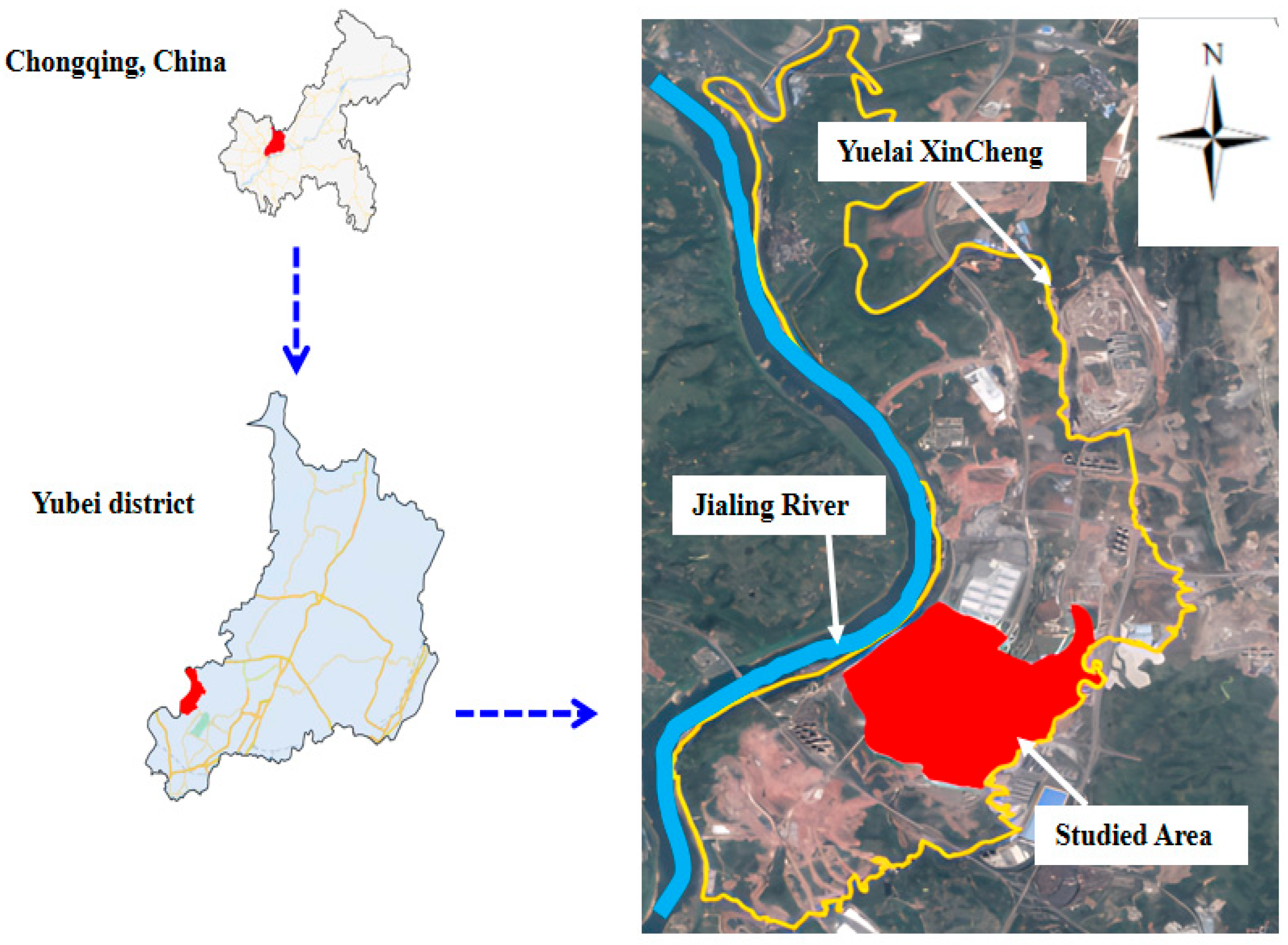
An SWMM model based on version 5.1.011 was developed for the study area. The study area is located in Yuelai Xincheng, Yubei District, Chongqing, a major metropolitan area in southwestern China (Figure 2). This watershed was selected due to its representative urban characteristics and the availability of comprehensive hydrological data. The area covers approximately 27 hectares with a single outlet, making it suitable for detailed hydrological analysis. Chongqing’s rapid urbanization and frequent urban flooding incidents make it an ideal case study for urban stormwater management research.
The region experiences a humid subtropical climate with an average annual temperature of 18.3 °C. The monthly average highest temperature reaches 28.1 °C in August, while the lowest is 5.7 °C in January. Historical precipitation data (2003–2013) show an average annual rainfall of 1078 mm, with approximately 69% occurring from May to September, creating distinct wet and dry seasons that are characteristic of many urban watersheds in similar climatic zones.

2.3. SWMM Model Parameters

This study focuses on the hydrological parameters in SWMM because the physical meanings of these parameters are not as straightforward as the hydraulic parameters. In total, there are eight key hydrological parameters within the SWMM model, shown in Table 1. Imperv (%) is the percent of impervious area; Width (m) is the width of the overland path; Slope (%) is the slope of the watershed; N-imperv and N-perv are the Manning’s n coefficients of the impervious and pervious areas, respectively; S-imperv (mm) and S-perv (mm) are the depression storage depths of the impervious and pervious areas, respectively; and Zero-imperv (%) is the percent of impervious area with zero storage. Of the eight parameters, two of them are related to the topographic features of the watershed, including Slope and Width. The rest of the parameters are related to types of land cover to account for the infiltration and surface storage, including Imperv, S-perv, S-imperv, Zero-imperv, N-perv, and N-imperv.
The key process in an SWMM hydrologic simulation is to solve a nonlinear routing equation that converts the rainfall excess to an outflow hydrograph [30]. The governing equation was derived from Manning’s Equation and the rectangular reservoir assumption and is shown in Equation (1).
Q = W · 1.49 n · h h p 5 / 3 · S 1 2
where Q is the runoff (m3/s); n is the land-cover Manning’s coefficient, including impervious land (N-imperv) and pervious land (N-perv); S is the slope (Slope); h is the surface rainfall excess depth that is associated with the parameters Imperv and Zero-imperv; hp is the maximum amount of surface storage loss that is associated with the parameters S-imperv and S-perv; and W is the width of the simplified rectangular watershed (Width).
True values and the typical parameter ranges are listed in Table 1. A uniform distribution within the parameter range is used as the prior distribution. Default values are used for all other parameters that are not included in this study. Default values recommended by the SWMM Reference Manual [26] were used for all other parameters not included in this study. The “true” parameter values used in this study were determined through a combination of field measurements, literature values for similar urban watersheds, and expert judgment. These values represent realistic conditions for the study area and were used to generate synthetic monitoring data for controlled numerical experiments.

2.4. Factors Impacting Calibration

(1)
Rainfall types
Both rainfall intensity and rainfall patterns are key characteristics of rainfall data. Hence, the impact of each was studied individually. The historical rainfall data used to construct the Intensity–Duration–Frequency (IDF) curves were obtained from the Chongqing Meteorological Bureau, covering a continuous record from 2003 to 2013. The return periods for different rainfall depths (Table 2) were determined through frequency analysis of the annual maximum rainfall series. Specifically, the Gumbel distribution was fitted to the series to estimate the rainfall depths corresponding to return periods ranging from 0.25 to 20 years. The Chicago hyetograph method was then applied to distribute the total rainfall depth into a time series with a peak intensity at the mid-point of the duration (for single-peak events).
To explore the influence of rainfall intensity on the parameter, nine single-peak rainfall events with return periods that ranged from 0.25 years to 20 years were investigated. The name, total depth, return period, and average intensity of each rainfall event are shown in Table 2.
To explore the influence of rainfall patterns, three types of rainfall patterns were studied, including single-peak, double-peak, and triple-peak patterns. The rainfall hyetographs for the single-peak, double-peak, and triple-peak rainfalls are shown in Figure 3, where P/P-total is the ratio of the rainfall depth at each time interval to the total rainfall depth.
(2)
Watershed hydrological characteristics
Regarding the influence of watershed hydrological characteristics, development level and the terrains of watersheds are the focus of this study. In the process of watershed development, natural hydrological characteristics change significantly [14]. The ratio of impervious surface increases [20] leads to a rapid increase in runoff. Furthermore, watershed slope, which represents the most significant terrain feature of a watershed, may impact the calibration as well. Therefore, it is critical to investigate the behavior of watersheds at different levels of development with different terrains in parameter calibration.
Three levels of impervious surface percentage were set: 20%, 50%, and 80%. In this study, watersheds at different levels of development are represented by three levels of impervious area percentage: 20%, 50%, and 80%, which represent low, medium, and high (fully developed) development levels, respectively. Watersheds in different terrains are represented by two sets of slopes, 0.4% and 4%. A slope of 0.4% represents a flat watershed, and a slope of 4% represents a steep watershed. This forms a combination of six hydrological characteristics, labeled Type 1–Type 6 and defined in Table 3.
Two typical slopes were used: 0.4% and 4%, which represent a flat watershed and a hilly watershed. The combination of development level and terrain leads to a total of six types of watersheds (labeled Type I–Type VI) as shown in Table 3.

2.5. Bayesian Inference and DREAM(zs) Sampling

Bayesian inference theory can be written as follows [8]:
p x Y = p x p Y x p Y p x L x Y
where x is an unknown parameter; Y is measured data; p x and p x Y are the prior probability density function and posterior probability density function, respectively; and L x Y is the likelihood function, indicating the degree of similarity between the model predictions and the measured data. The model predictions are obtained by running an SWMM simulation with a given parameter vector. Equation (2) indicates that the posterior distribution of the unknown parameters can be estimated through the prior distribution, measured data, and likelihood function based on the Bayesian theory. In model calibration, the prior distribution, p x , is typically known. Hence, the posterior distribution, p x Y , is mainly determined by the likelihood function, L x Y .
The likelihood function can be calculated based on the following formula [31,32]. Uncertainties from field measurement error and SWMM numerical simulation are reflected in the likelihood function by assuming that the composite errors follow a Gaussian distribution with a mean of zero and a standard deviation of σ.
L x Y = t = 1 n 1 2 π σ ^ t 2 e x p 1 2 y t y ~ t ( x ) σ ^ t 2
where L x Y is the likelihood function, indicating the degree of similarity between the model predictions and the measured data; n is the total number of data points in the observed hydrograph; and σ ^ t is the standard deviation of the error at time t. This term quantifies the combined uncertainty from field measurement errors and the SWMM model structure, assumed to follow a Gaussian distribution with a mean of zero; y t is the observed flow rate at time t (i.e., the “monitoring” data); and y ~ t ( x ) is the simulated flow rate at time t, obtained by running the SWMM model with the parameter set x.
Most hydrological models are nonlinear, which means that p x Y in Equation (3) cannot be solved analytically. To overcome this, Equation (3) is usually solved in an indirect way through sampling methods such as the Monte Carlo method. However, traditional Monte Carlo sampling is low in efficiency because it evaluates all the possible values. To improve the sampling efficiency, advanced sampling algorithms have been developed, such as Markov Chain Monte Carlo Metropolis–Hastings (MCMC M-H) [8] and MCMC Differential Evolution Adaptive Metropolis (DREAM) [33]. MCMC sampling has the advantage of efficiently extracting samples based on the computed posterior distribution, which reduces the computational efforts and speeds up the inference process significantly [29].
Compared to the traditional MCMC M-H algorithm, MCMC-DREAM(zs) further improves the computational efficiency by automatically adjusting the walking size and searching directions based on historical sampling information. MCMC-DREAM(zs) also contains multiple Markov chains that make it possible to explore the parameter space simultaneously. This feature makes the sampling algorithm easy to parallelize as well, and hence could further boost the algorithm efficiency. The MCMC-DREAM(zs) sampling algorithm has shown an excellent sampling efficiency in complex, high-dimensional, and multi-modal target distribution [34]. This is particularly useful in SWMM parameter calibrations, as it is a high-dimensional problem. Equation (4) is used to determine the walking size of the ith MCMC-DREAM(zs) chain [29].
d X i = ζ d * + 1 d * + λ d * γ δ , d * j = 1 δ ( Z a j Z b j )
where d is the number of parameters; m is the number of parameters taken from the historical sampling results; Z = z 1 , , z m is an m × d matrix that contains the sampling results from N MCMC chains; γ = 2.38 2 δ d * represents the jump rate, where δ is the number of chain pairs used to generate the jump; λ d *   a n d   ζ d * are taken randomly from the uniform distribution, U (−0.1, 0.1), and the normal distribution, N (0, c * ), respectively, where c * is a number smaller than the target distribution width (10–12), and a and b are the non-repeated sampling results from the unit of {1,…, m} [29]. The new proposed value is calculated by Equation (5).
X p i = X t 1 i + d X i
Then, an accepting probability is calculated based on the proposed value using Equation (6) [31].
p a c c X t 1 i X p i = m i n 1 , p ( X p i , Y ) p X t 1 , i , Y
where p ( X p i , Y ) and p ( X t 1 i , Y ) represent the new probability and the current probability on the ith chain, respectively. p a c c ( X t 1 i X p i ) is the accepting probability of assigning X p i to X t 1 i . The following accept–reject rule in Equation (7) is typically used to determine if the proposed new value of X p i will be accepted or not [31].
p a c c ( X t 1 i X p i ) U ( 0,1 )
where U(0,1) is a random value generated from the uniform distribution U ( 0,1 ) . If the proposed value is accepted, the Markov chain advances to a new value of X p i from the current value of X t 1 i , otherwise the proposed value will be discarded.

2.6. Calibration Performance Indicators

(1)
Criteria of Convergence
DREAM(zs) uses multiple Markov chains to simultaneously sample the parameter space. According to the Markov chain theory, the posterior distribution of the parameters could converge to a stable distribution after sufficient iterations. Convergence of the sampling process to a stable posterior probability distribution for multiple chain sampling was evaluated using the R statistic index defined by Gelman and Rubin [12], where an R j 1.2 indicates that the sampling converges to a stable solution. The formula for R is shown in Equation (8).
R j = N + 1 N σ ^ 2 ( j ) W j T 2 N T
where W j is the variance of the parameter j in each chain, σ ^ 2 ( j ) is the estimated variance of the target distribution of the jth parameter, N is the numbers of chains, and T is the total sampling time for each chain.
The root mean square error (RMSE), Nash efficiency coefficient (NSE), and deviation percentage (PBIAS) were chosen to evaluate the approximate values of the numerical predictions and the measured values. In the computation of the deviation percentage (PBIAS), both total runoff volume and peak flow rate at all time steps are calculated. Calculations of these indicators are shown in Equations (9)–(11):
R M S E = 1 n t = 1 n ( Y i Y ~ i ) 2
N S E = 1 t = 1 n Y i Y ~ i 2 t = 1 n Y i Y ¯ 2
P B I A S = t = 1 n Y i t = 1 n Y ~ i t = 1 n Y i × 100
where n is the total number of compared data points picked on the hydrograph, Y i is the model simulation result at the ith data point, and Y ~ i is the simulated value at the ith data point.
(2)
Accuracy of calibrated parameters
The results of the Bayesian DREAM(zs) calibration are presented using posterior probability distributions. The narrower the posterior distribution, the better the calibration results. If the posterior distribution does not show an obvious peak, it indicates that the true value of the parameter is difficult to distinguish from the calibration process. The standard deviation (SD) and coefficient of variation (Cv) are chosen as measures to evaluate the discreteness of the posterior distribution, as shown in Equations (12) and (13). Both indicate whether the calibrated results are closely clustered together or spread widely. Small values imply a narrow distribution, with results clustered around the specific values tightly.
S D = 1 n t = 1 n ( x i X ¯ ) 2
C v = S D X ¯
where n is the total number of compared data points picked on the hydrograph, x i is the value of the parameter, and X ¯ is the mean value of the posterior distribution.

3. Results and Discussion

3.1. Identifying the Optimal Rainfall Intensity for Robust SWMM Calibration

In this section, to isolate the effects of rainfall intensity on each parameter, the parameters were calibrated individually, i.e., only one parameter was calibrated for each rainfall intensity. The parameter sampling trajectories derived from the Bayesian DREAM(zs) calibration algorithm for rainfalls R1–R9 were plotted and included in Figure S4 in the Supplementary Materials. It can be seen that all sampling trajectories are relatively discrete at the beginning of the iteration and become concentrated as the MCMC sampling progresses. Analysis of the R statistic index history (Figure S4 in the Supplementary Materials) defined in Equation (4) shows that when the sampling times reach 5000, the R statistic drops below 1.2 in all cases. As described in Section 2.3, this means the Bayesian DREAM(zs) calibration algorithm converges under all rainfall events. This indicates that the developed Bayesian DREAM(zs) SWMM calibration framework is robust. However, it can be seen from Figure 4 that the sampling range of each parameter varies significantly with different rainfall intensities. Taking parameter S-perv as an example, the sampling value varies within the ±50% range for the R3 and R7 rainfall intensities, while it varies within the range of ±20% for R5. The same trend can be observed for all other parameters. For all three rainfalls, rainfall R5 produces the most concentrated sampling trajectories. Additionally, Figure 4 shows that for the same rainfall, the sampling trajectories of each parameter show different patterns. The parameters Imperv and S-imperv have the narrowest sampling trajectories, which are approximately straight lines with fluctuations within the ±5% and ±10% ranges, respectively. This indicates that these two parameters are relatively easy to calibrate to the true value. The sampling trajectories of the parameters S-perv and Zero-imperv are somewhat concentrated, with a fluctuation range of approximately 20%. The sampling trajectories of the rest of the five parameters are quite diffusive, with a fluctuation range of over 50%.
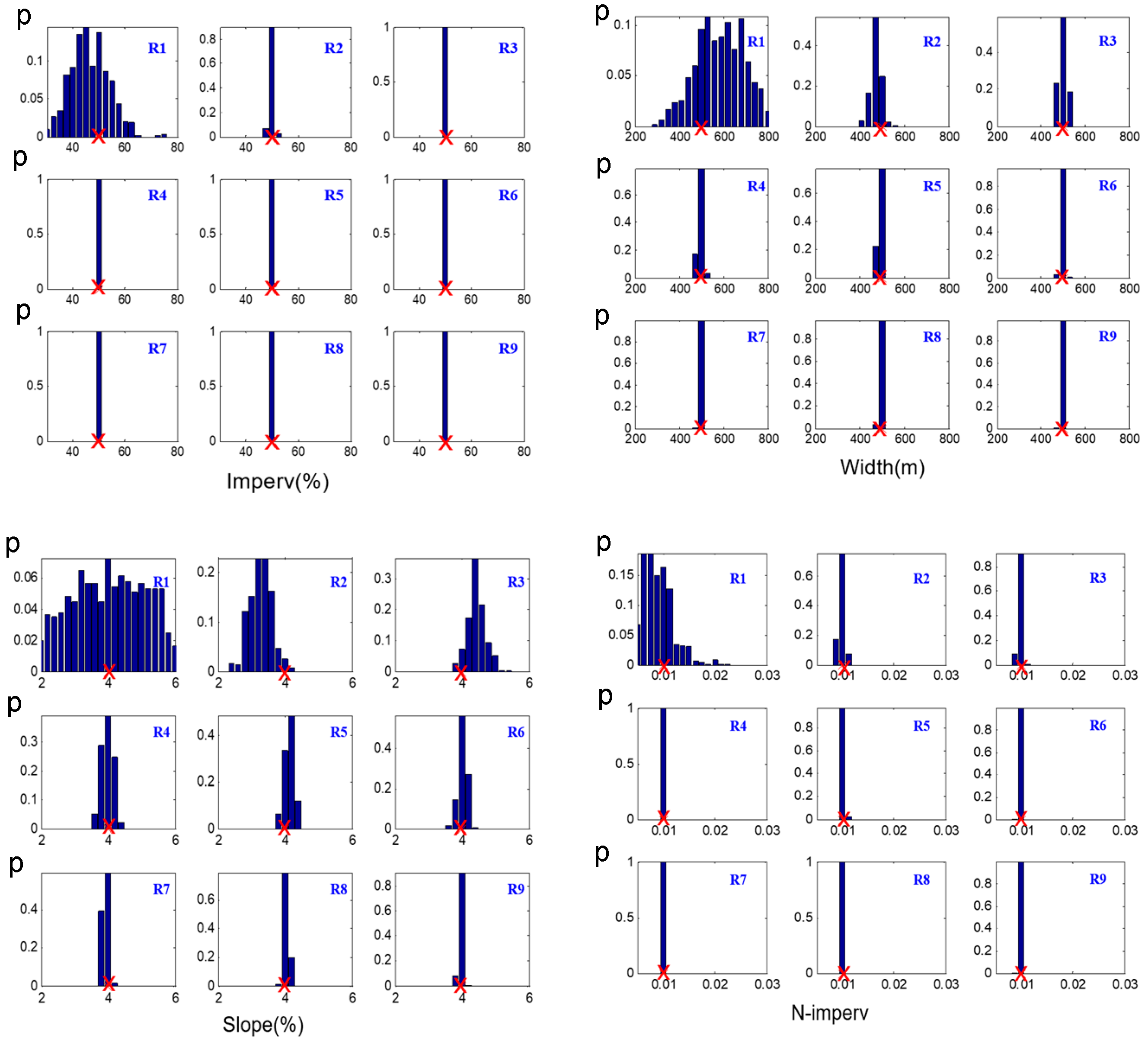
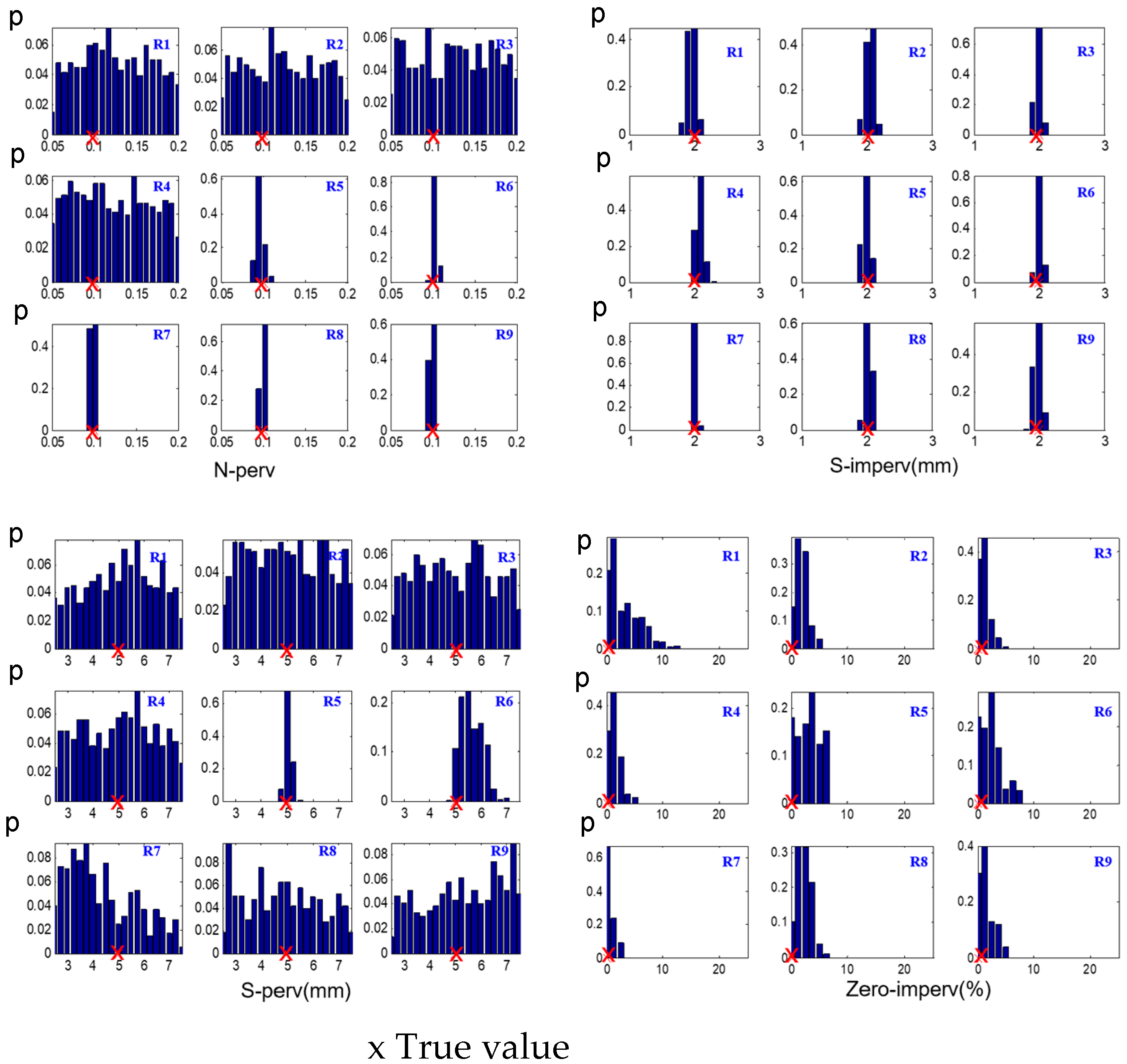
The posterior probability distributions of all parameters under nine rainfall intensities, plotted in Figure 5, also show the same trend. Based on the definition of probability distributions, a narrow probability distribution indicates that the sampling results are concentrated closely around a central value, resulting in a small range of possible values and higher accuracy. On the contrary, a wide flat distribution indicates less accurate results. In Figure 5, it can be seen that the posterior probability distributions of all parameters are around the “true value”, which is depicted with a red cross, and the probability distributions under low-intensity rainfalls (R1–R4) are generally wider and flatter than the corresponding ones under higher-intensity rainfalls (R5–R9), except for the parameter S-imperv. This indicates that the calibration results obtained using low-intensity rainfalls are less accurate for these parameters, while S-imperv can be calibrated to true values regardless of the rainfall intensities. Figure S3 also shows that, under rainfall intensity R5, the narrowest probability distribution can be observed for all parameters except Zero-imperv. Under this rainfall intensity, the probability of “the result being the true value” is approximately 0.5 for Slope, 0.6 for S-imperv and N-perv, 0.65 for S-perv, and above 0.8 for Imperv, Width, and N-imperv. This means that all parameters can be calibrated to the true values under rainfall intensity R5, which is medium. For the parameters Imperv, Width, and N-imperv, the calibration performance is generally good if the rainfall event has an intensity equal to or higher than R3, indicated by a probability of yielding a true value of 0.6 or higher. It could also be observed that the accuracy of the parameters Slope and N-perv improves significantly as the rainfall intensity increases, indicated by the probability of yielding a true value increasing from 0.06 to 0.6 or higher. Hence, regarding the eight parameters, except for S-perv, all could be calibrated to true values by storms with a medium or higher intensity. The parameter S-perv could be calibrated well only by a medium- or high-intensity storm. It can be concluded that the medium-intensity rainfall (R5), which is equivalent to a one-year-return-period storm, produces the most satisfying calibration results overall.
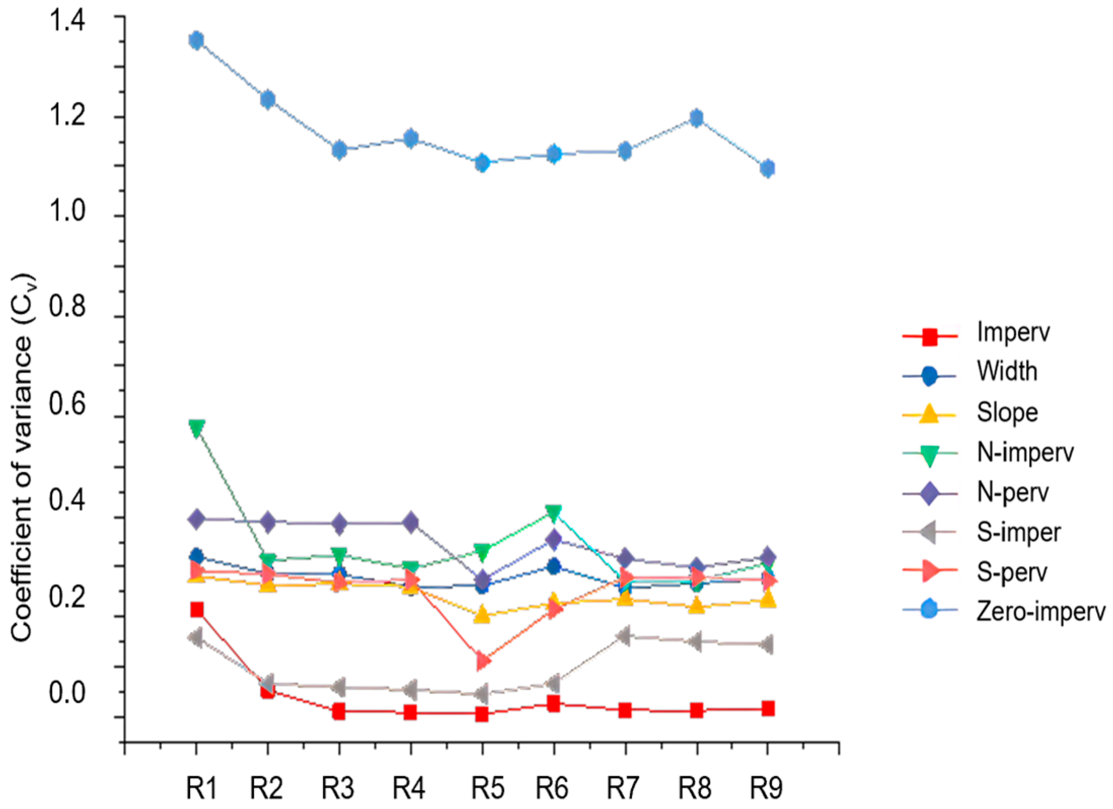
To further quantitively evaluate the overall performances of all nine rainfall intensities, statistical indexes, including the mean, median, standard deviation, and coefficient of variation of the posterior distribution, under nine rainfalls were calculated for each parameter. The coefficient of variation can reflect the degree of dispersion of the posterior distribution. The smaller the coefficient of variation, the closer the parameter to the mean value, suggesting a high degree of confidence in the expected results. The coefficient of variation for each parameter posterior distribution under the nine rainfalls is plotted in Figure 5, with the statistic indexes for rainfall R5 listed in Table 3 as examples. A posterior distribution box map that shows the mean values of the calibration and the true values is provided in the Supplementary Materials, Figure S6. It can be seen that the overall results produced by rainfalls R3 though R5 show good agreement with the true values. Taking the convergency effect into consideration, R5 is considered to have the best performance for all nine rainfall intensities. It can be observed from Figure 5 and Table 4 that, regarding the uncertainty of the parameters in the calibration, they rank from low to high as follows: Imperv < S-imperv < S-perv < Slope < Width < N-imperv < N-perv < Zero-imperv, where a low uncertainty indicates that an accurate calibration is easier to reach. This finding agrees with the physical meaning of these parameters. The result is consistent with the conclusions of previous research works. For example, Muleta [15] used 7-day rainfall data with a low-intensity rainfall like R1 and concluded that only Imperv, S-imperv, and Zero-imperv were sensitive. In an uncertainty study of peak and total flow volume predicted by the SWMM model, Sun [28] also noticed that the parameters are not sensitive to low rainfall intensities.

3.2. Impacts of Rainfall Pattern

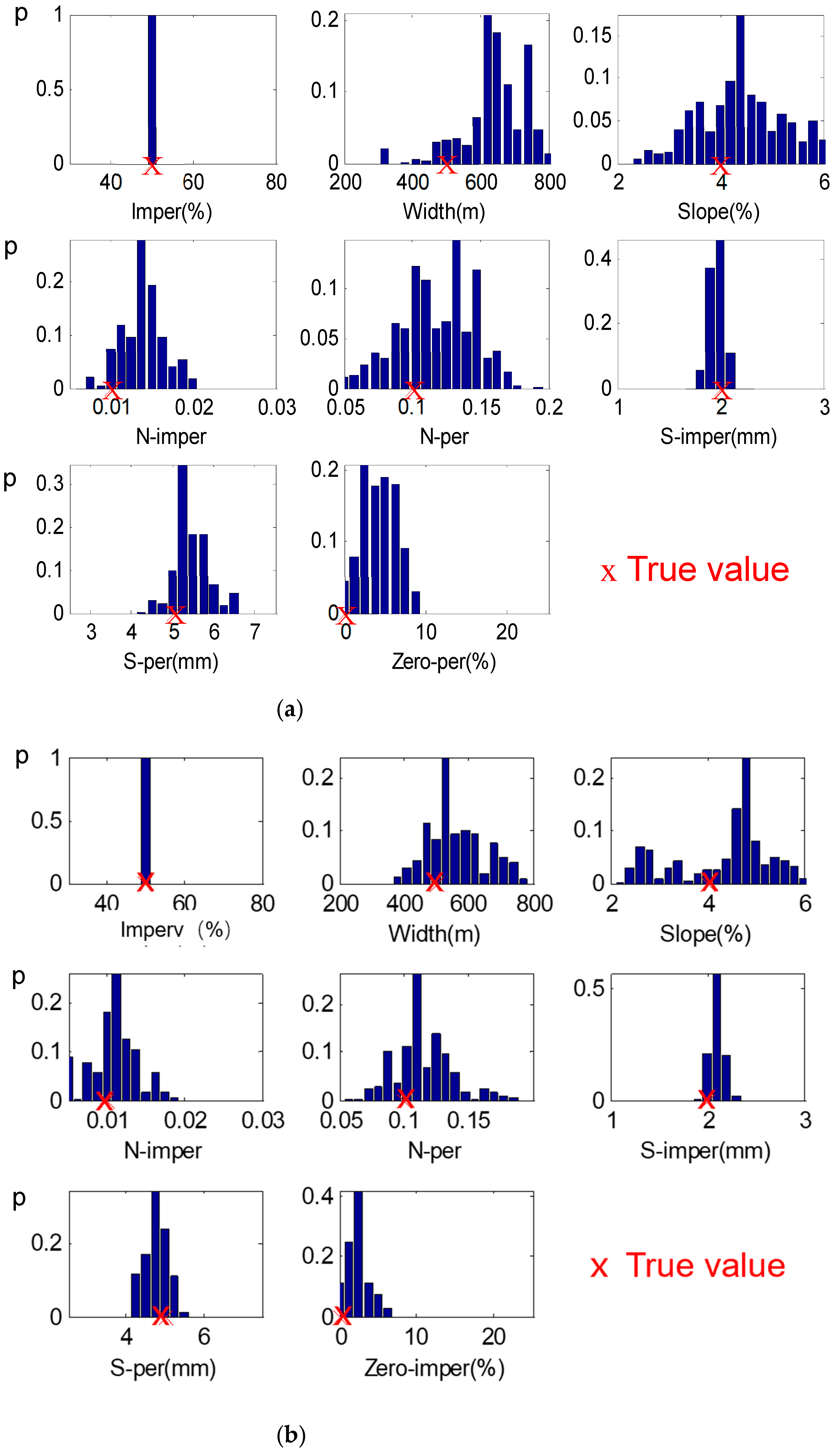
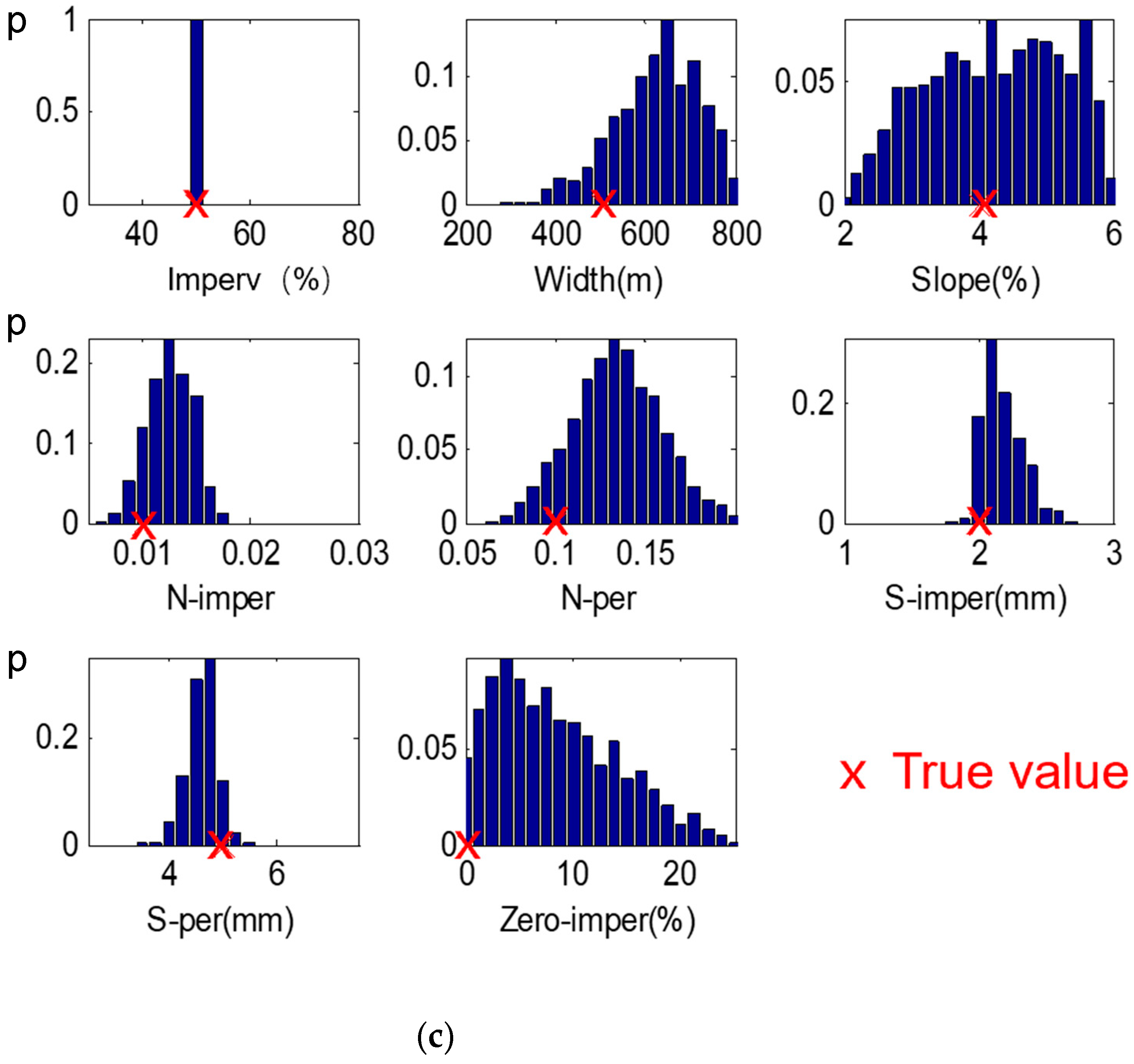
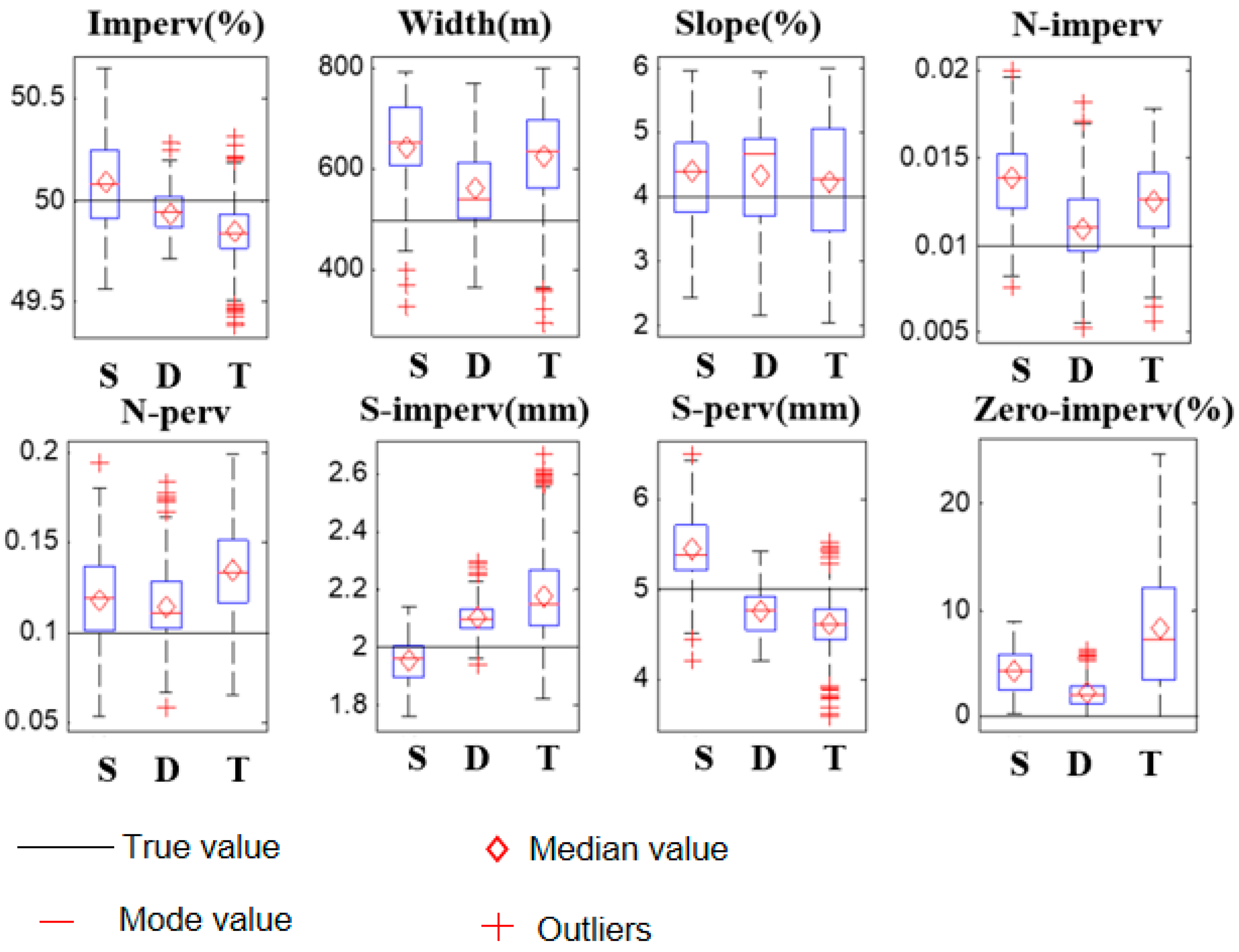
Besides rainfall intensity, parameter calibration under different rainfall patterns, including single-peak, double-peak, and triple-peak patterns, were investigated. In this section, all eight parameters were calibrated simultaneously. Based on the findings from Section 3.1, all three patterns have a rainfall intensity equivalent to rainfall R5. The posterior distributions under all three rainfall patterns are shown in Figure 6, and a box plot is shown in Figure 7.
Comparing Figure 6a to Figure 4, it can be seen that when eight parameters are calibrated simultaneously, the calibration accuracy decreased compared to the individual calibration in Section 3.1, especially for the parameters Slope and Width. In the individual calibration, both parameter probability distributions are narrowly centered around the true value with peak probabilities of 0.5 and 0.7, respectively, indicating a high likelihood of a result occurring near the true value. However, when calibrated simultaneously, the probability distribution is much flatter, and the probability of the result being near the true value dropped below 0.1 in both cases. This is because of the strong correlation between the parameters, especially between Width and Slope. Accurate calibration of these parameters poses great challenges.
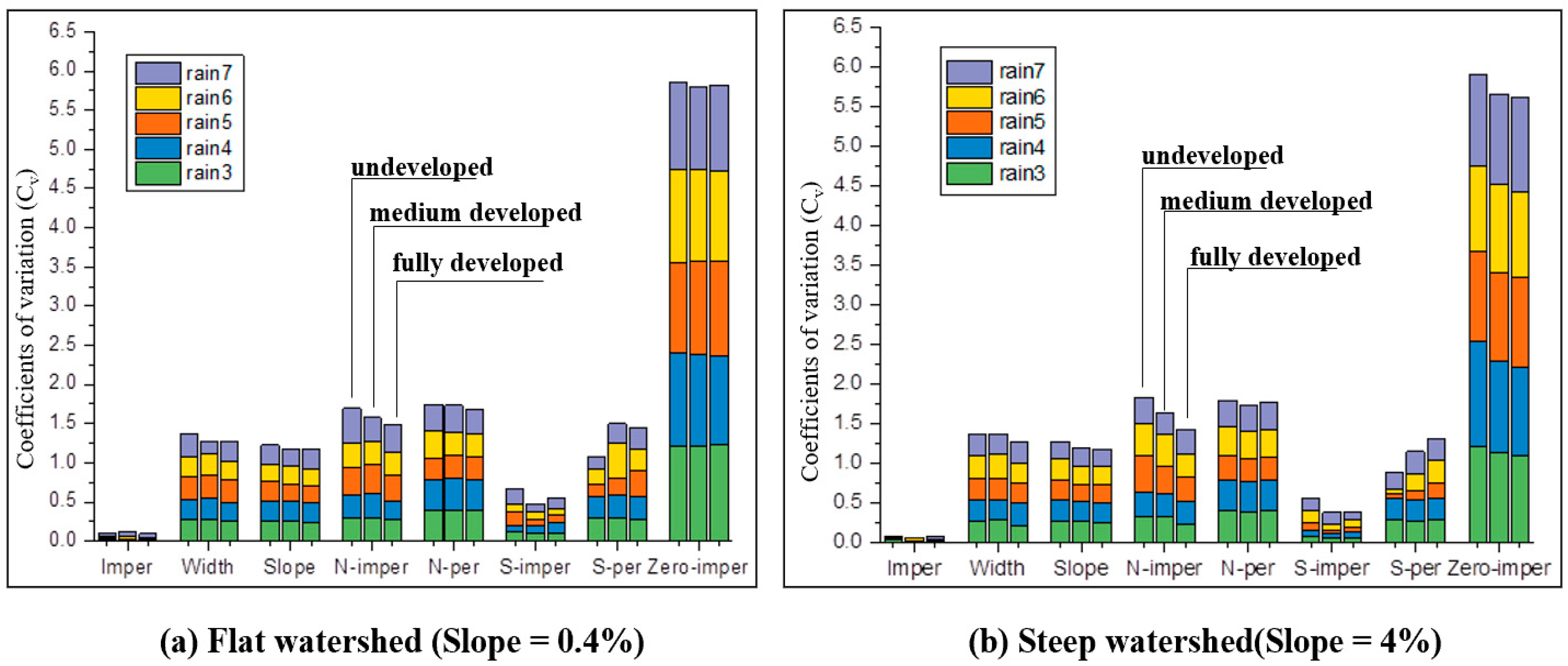
However, Figure 7 shows that using a double-peak rainfall pattern remedies some of the above problems. It can be seen from Figure 7 that rainfall pattern has a great influence on the parameters, and the probability distribution produced for the double-peak rainfall pattern is the narrowest compared to the distributions for the single-peak and triple-peak rainfall patterns, especially for the parameter Width. The narrowest distribution indicates the best calibration result. The corresponding standard deviation (Table 5) also confirms this quantitively.
This finding is important for urban flooding analysis and mitigation measurements. Based on the level-pool flow routing theory employed by the SWMM hydrological module [30], the Width and Slope of a watershed respectively determine the distance and velocity of the unit hydrograph to be routed to the watershed outlet. They both affect the travel time of the unit hydrograph. Consequently, they directly determine the peak flow rate and the hydrograph shape at the watershed outlet. Hence, the accuracies of Width and Slope are critical for predicting the peak flow rate for flooding control purposes. Results from this study suggest that a double-peak rainfall could be used to distinguish the two parameters and produce a more accurate Width calibration. This sheds lights on the selection of the calibration storm data used for these parameters.

3.3. Impacts of Watershed Hydrological Characteristics

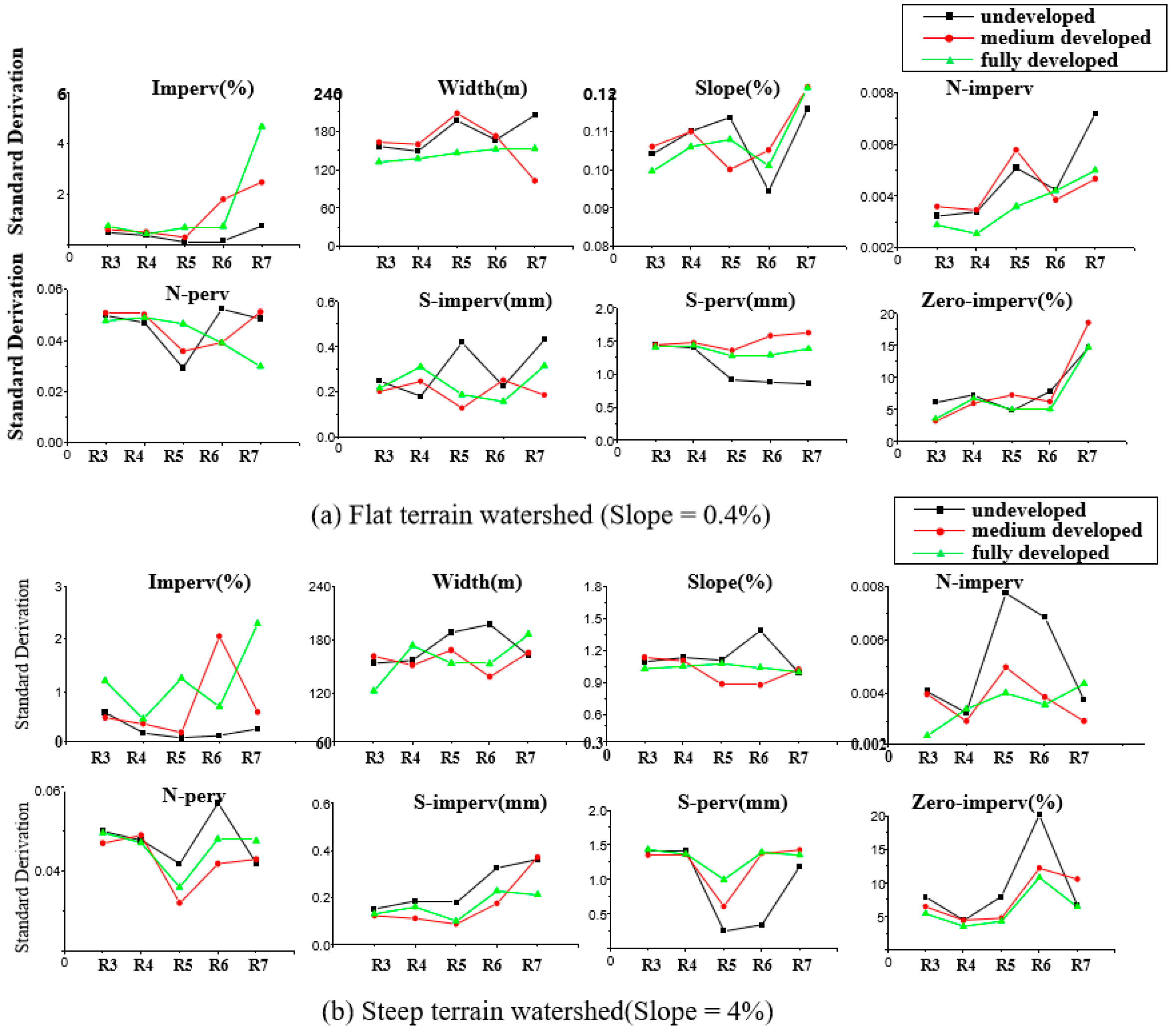
As shown in Section 3.1, in general, the calibration results become more satisfying as the rainfall intensity goes up. This is partially due to the higher runoff volume produced by heavier rainfalls. This indicates that the development level of a watershed, or the percentage of impervious land, might affect the accuracy of parameters when different rainfall data are used. As revealed in Section 3.1, parameters are not sensitive when rainfall intensity is too low. Hence, only rainfalls with a medium or higher intensity (R3–R7) are investigated in this section. Coefficients of variation of different rainfall events under various watershed conditions are shown in Figure 8. The overall performances of parameter calibrations for different watersheds are shown in Figure 8 and are presented in the Supplementary Materials (Figures S3–S8). The standard deviation of each parameter is plotted in Figure 9.
Comparing Figure 8a and Figure 8b, it can be found that the mean values, standard deviations, and coefficients of variance of the calibrated results are similar between flat and steep watersheds, with the same development level for each individual rainfall pattern. This indicates that the terrain of the watershed is not a sensitive factor in the selection of calibration rainfall data.
From Figure 9, it can be seen that the parameter calibration results are similar at all development levels for rainfall intensities lower than R5, although parameter calibration performance varies slightly for rainfalls with higher intensities. This means the development level of a watershed somewhat affects what type of rainfall data is best for calibration. Overall, most parameters could be calibrated better using low- to medium-intensity rainfalls, such as R4, R5, and R6, for all three development levels. The standard deviation increases rapidly as the rainfall intensity rises higher than R6. Overall, a fully developed watershed yields more satisfyingly calibrated parameters, except for S-perv, compared to undeveloped and medium-developed watersheds. This finding is reasonable, as the parameter S-perv is the surface depression storage on pervious land and does not impact the peak or hydrograph much in a fully developed watershed.
It can also be observed from Figure 9 that, for peak flow rate calibration purposes, for parameters that have a high impact on peak flows [27], including imperv, Width, Slope, N-imperv, and Zero-imperv, it is more appropriate to choose rainfall events with a medium or a slightly high intensity. Rainfall events with an intensity higher than R6 should be avoided for all developmental levels. For total flow volume calibration purposes, for parameters that are key to flow volume, including imperv %, S-imperv, S-perv, and Zero-imperv, a medium rainfall intensity such as R5 should be used for all developmental levels.

4. Conclusions

This study developed a Bayesian SWMM calibration framework incorporating an advanced DREAM(zs) sampling method and systematically investigated the influences of rainfall data and watershed characteristics on SWMM parameter calibration precision. Through controlled numerical experiments, the behaviors of eight key hydrological parameters were scrutinized. The main findings, supported by quantitative evidence, are summarized as follows:
(1)
Rainfall data with a medium intensity equivalent to a one-year return period (R5, total depth of 42.70 mm) or higher generally yielded the most satisfactory parameter accuracy. Compared to low-intensity rainfalls (e.g., R1), using the R5 rainfall reduced the posterior distribution standard deviations for most parameters by 40% to 60%. Notably, the parameters Imperv, S-imperv, and N-imperv exhibited minimal sensitivity to rainfall intensity variations, maintaining high accuracy across all scenarios (e.g., Imperv’s coefficient of variation remained below 0.005). The difficulty of achieving accurate calibration for all parameters, ranked from easiest to most challenging based on their posterior distribution coefficients of variation, was as follows: Imperv (Cv ≈ 0.005) < S-imperv (Cv ≈ 0.045) < S-perv (Cv ≈ 0.112) < Slope (Cv ≈ 0.202) < Width (Cv ≈ 0.262) < N-imperv (Cv ≈ 0.332) < N-perv (Cv ≈ 0.274) < Zero-imperv (Cv ≈ 1.108).
(2)
The double-peak rainfall pattern produced the most satisfactory calibration results. It was particularly effective in distinguishing between strongly correlated parameters like Width and Slope. Quantitatively, using the double-peak pattern reduced the standard deviation of the Width parameter from 168.647 m (single-peak) to 110.789 m, an improvement of approximately 34%. Similarly, the standard deviation of N-perv decreased from 0.032 to 0.021.
(3)
Watershed hydrological characteristics (terrain and development level) exhibited a negligible influence on parameter calibration accuracy once an optimal rainfall event (intensity and pattern) was selected. The differences in performance metrics (e.g., coefficient of variation) across different watershed types were minimal. For instance, the coefficient of variation for the key parameter Imperv remained in a narrow range (0.004 to 0.007) regardless of watershed type or rainfall intensity, confirming that watershed characteristics are not a dominant factor.
In conclusion, this study demonstrates that the a priori selection of rainfall events—specifically, one-year-return-period, double-peak storms—can significantly enhance the accuracy and reliability of SWMM parameter calibration. These insights provide actionable guidance for modelers in selecting calibration data tailored to specific management objectives, such as flood control or pollution management. The developed Bayesian DREAM(zs) framework also serves as a robust tool for future uncertainty analyses in urban water resources modeling.

Supplementary Materials

The following supporting information can be downloaded at https://www.mdpi.com/article/10.3390/w17233435/s1: Figure S1. The R-statistics and RMSE trajectories during sampling; Figure S2. The theoretical and Bayesian inferred posterior distributions; Figure S3. The sampling trajectory of each parameter in the calibration process; Figure S4. The R-statistic trajectory in the sampling process; Figure S5. The posterior distribution box map of studied parameters; Figure S6. The posterior distribution of eight parameters in various rainfalls (Type 1); Figure S7. The posterior distribution of eight parameters in various rainfalls (Type 2); Figure S8. The posterior distribution of eight parameters in various rainfalls (Type 3); Figure S9. The posterior distribution of eight parameters in various rainfalls (Type 4); Figure S10. The posterior distribution of eight parameters in various rainfalls (Type 5); Figure S11. The posterior distribution of eight parameters in various rainfalls (Type 6).

Author Contributions

Conceptualization, Z.S.; supervision, Z.S.; original draft, Z.S.; methodology, X.Z.; formal analysis, X.Z.; writing—review and editing, J.W., J.D. and S.Y. All authors have read and agreed to the published version of the manuscript.

Funding

This research work was financially supported by the National Key R&D Program of China, the Ministry of Science and Technology, PR China (Grant No. 2022YFC3800500). We also acknowledge the support of the Chongqing Key R&D Program (CSTB2023TIAD-KPX0079).

Data Availability Statement

The data presented in this study are openly available at https://github.com/dztsz/my-first-project (accessed on 7 April 2025).

Conflicts of Interest

The authors declare no conflicts of interest.

Nomenclature

Abbreviations:
SWMMStorm Water Management Model
DREAM(zs)Differential Evolution Adaptive Metropolis, Version ZS
MCMCMarkov Chain Monte Carlo
GLUEGeneralized Likelihood Uncertainty Estimation
IDFIntensity–Duration–Frequency
RMSERoot Mean Square Error
NSENash–Sutcliffe Efficiency Coefficient
PBIASPercentage Bias
CvCoefficient of Variation
SDStandard Deviation
pProbability Density
SWMM Model Parameters:
ImpervPercent of impervious area (%)
WidthWidth of overland flow path (m)
SlopeAverage slope of the sub-catchment (%)
N-impervManning’s roughness coefficient for impervious areas
N-pervManning’s roughness coefficient for pervious areas
S-impervDepression storage depth for impervious areas (mm)
S-pervDepression storage depth for pervious areas (mm)
Zero-impervPercent of impervious area with no depression storage (%)

References

  1. Aqil, M.; Kita, I.; Yano, A.; Nishiyama, S. Analysis and prediction of flow from local source in a river basin using a Neuro-fuzzy modeling tool. J. Environ. Manag. 2007, 85, 215–223. [Google Scholar] [CrossRef]
  2. Azzellino, A.; Cevirgen, S.; Giupponi, C.; Parati, P.; Ragusa, F.; Salvetti, R. SWAT meta-modeling as support of the management scenario analysis in large watersheds. Water Sci. Technol. 2015, 72, 2103–2111. [Google Scholar] [CrossRef]
  3. Ball, J.E.; Fang, T. Evaluation of spatially variable control parameters in a complex catchment modelling system: A genetic algorithm application. J. Hydroinformatics 2007, 9, 163–173. [Google Scholar] [CrossRef]
  4. Barco, J.; Wong, K.M.; Stenstrom, M.K. Automatic Calibration of the U.S. EPA SWMM Model for a Large Urban Catchment. J. Hydrol. Eng. 2008, 134, 466–474. [Google Scholar] [CrossRef]
  5. Beven, K.; Binley, A. The future of distributed models-model calibration and uncertainty prediction. Hydrol. Process. 1992, 6, 279–298. [Google Scholar] [CrossRef]
  6. Beven, K.; Freer, J. Equifinality, data assimilation, and uncertainty estimation in mechanistic modelling of complex environmental systems using the GLUE methodology. J. Hydrol. 2001, 249, 11–29. [Google Scholar] [CrossRef]
  7. Dai, H.; Ye, M. Variance-based global sensitivity analysis for multiple scenarios and models with implementation using sparse grid collocation. J. Hydrol. 2015, 528, 286–300. [Google Scholar] [CrossRef]
  8. Delle Monache, L.; Lundquist, J.K.; Kosovic, B.; Johannesson, G.; Dyer, K.M.; Aines, R.D.; Chow, F.K.; Belles, R.D.; Hanley, W.G.; Larsen, S.C.; et al. Bayesian Inference and Markov Chain Monte Carlo Sampling to Reconstruct a Contaminant Source on a Continental Scale. J. Appl. Meteorol. Clim. 2008, 47, 2600–2613. [Google Scholar] [CrossRef]
  9. Li, C.; Wang, W.; Xiong, J.; Chen, P. Sensitivity Analysis for Urban Drainage Modeling Using Mutual Information. Entropy 2014, 16, 5738–5752. [Google Scholar] [CrossRef]
  10. Zhan, C.-S.; Song, X.-M.; Xia, J.; Tong, C. An efficient integrated approach for global sensitivity analysis of hydrological model parameters. Environ. Model. Softw. 2013, 41, 39–52. [Google Scholar] [CrossRef]
  11. Song, X.; Zhan, C.; Kong, F.; Xia, J. Advances in the study of uncertainty quantification of large-scale hydrological modeling system. J. Geogr. Sci. 2011, 21, 801–819. [Google Scholar] [CrossRef]
  12. Dotto, C.B.; Mannina, G.; Kleidorfer, M.; Vezzaro, L.; Henrichs, M.; McCarthy, D.T.; Freni, G.; Rauch, W.; Deletic, A. Comparison of different uncertainty techniques in urban stormwater quantity and quality modelling. Water Res. 2012, 46, 2545–2558. [Google Scholar] [CrossRef] [PubMed]
  13. Dotto, C.B.S.; Kleidorfer, M.; Deletic, A.; Rauch, W.; McCarthy, D.T. Impacts of measured data uncertainty on urban stormwater models. J. Hydrol. 2014, 508, 28–42. [Google Scholar] [CrossRef]
  14. Baker, E.A.; Manenti, S.; Reali, A.; Sangalli, G.; Tamellini, L.; Todeschini, S. Combining noisy well data and expert knowledge in a Bayesian calibration of a flow model under uncertainties: An application to solute transport in the Ticino basin. Int. J. Geomath. 2023, 14, 8. [Google Scholar] [CrossRef]
  15. Muleta, M.K.; McMillan, J.; Amenu, G.G.; Burian, S.J. Bayesian Approach for Uncertainty Analysis of an Urban Storm Water Model and Its Application to a Heavily Urbanized Watershed. J. Hydrol. Eng. 2013, 18, 1360–1371. [Google Scholar] [CrossRef]
  16. Liu, S.M.; Che, H.; Smith, K.; Lei, M.S.Z.; Li, R.N. Performance evaluation for three pollution detection methods using data from a real contamination accident. J. Environ. Manag. 2015, 161, 385–391. [Google Scholar] [CrossRef]
  17. Gelman, A.; Rubin, D.B. Inference from Iterative Simulation Using Multiple Sequences. Stat. Sci. 1992, 7, 457–472. [Google Scholar] [CrossRef]
  18. Gironás, J.; Roesner, L.A.; Rossman, L.A.; Davis, J. A new applications manual for the Storm Water Management Model (SWMM). Environ. Model. Softw. 2010, 25, 813–814. [Google Scholar] [CrossRef]
  19. Madrazo-Uribeetxebarria, E.; Garmendia, M.; Berrondo, J.A.; Andrés-Doménech, I. Sensitivity analysis of permeable pavement hydrological modelling in the storm water management model. J. Hydrol. 2021, 600, 126525. [Google Scholar] [CrossRef]
  20. Smith, T.J.; Marshall, L.A. Bayesian methods in hydrologic modeling: A study of recent advancements in Markov chain Monte Carlo techniques. Water Resour. Res. 2008, 44, W00B05. [Google Scholar] [CrossRef]
  21. Jacobson, C.R. Identification and quantification of the hydrological impacts of imperviousness in urban catchments: A review. J. Environ. Manag. 2011, 92, 1438–1448. [Google Scholar] [CrossRef]
  22. Zhuang, Q.; Li, M.; Lu, Z. Assessing runoff control of low impact development in Hong Kong’s dense community with reliable SWMM setup and calibration. J. Environ. Manag. 2023, 345, 118599. [Google Scholar] [CrossRef]
  23. Jia, H.; Xu, T.; Liang, S.; Zhao, P.; Xu, C. Bayesian framework of parameter sensitivity, uncertainty, and identifiability analysis in complex water quality models. Environ. Modell. Softw. 2018, 104, 13–26. [Google Scholar] [CrossRef]
  24. Tanim, A.H.; Smith-Lewis, C.; Downey, A.R.J.; Imran, J.; Goharian, E. Bayes_Opt-SWMM: A Gaussian process-based Bayesian optimization tool for real-time flood modeling with SWMM. Environ. Model. Softw. 2024, 179, 106122. [Google Scholar] [CrossRef]
  25. Kleidorfer, M.; Deletic, A.; Fletcher, T.D.; Rauch, W. Impact of input data uncertainties on urban stormwater model parameters. Water Sci. Technol. 2009, 60, 1545–1554. [Google Scholar] [CrossRef]
  26. Macdonald, N.; Redfern, T.; Miller, J.; Kjeldsen, T.R. Understanding the impact of the built environment mosaic on rainfall-runoff behaviour. J. Hydrol. 2022, 604, 127147. [Google Scholar] [CrossRef]
  27. Li, Q.; Wang, F.; Yu, Y.; Huang, Z.; Li, M.; Guan, Y. Comprehensive performance evaluation of LID practices for the sponge city construction: A case study in Guangxi, China. J. Environ. Manag. 2019, 231, 10–20. [Google Scholar] [CrossRef]
  28. Song, X.M.; Zhang, J.Y.; Zhan, C.S.; Xuan, Y.Q.; Ye, M.; Xu, C.G. Global sensitivity analysis in hydrological modeling: Review of concepts, methods, theoretical framework, and applications. J. Hydrol. 2015, 523, 739–757. [Google Scholar] [CrossRef]
  29. Sun, N.; Hong, B.; Hall, M. Assessment of the SWMM model uncertainties within the generalized likelihood uncertainty estimation (GLUE) framework for a high-resolution urban sewershed. Hydrol. Process. 2014, 28, 3018–3034. [Google Scholar] [CrossRef]
  30. Rossman, L.A.; Huber, W.C. Storm Water Management Model Reference Manual Volume I—Hydrology; U.S. EPA Office of Research and Development: Washington, DC, USA, 2016.
  31. Vrugt, J.A.; ter Braak, C.J.F.; Diks, C.G.H.; Robinson, B.A.; Hyman, J.M.; Higdon, D. Accelerating Markov Chain Monte Carlo Simulation by Differential Evolution with Self-Adaptive Randomized Subspace Sampling. Int. J. Nonlinear Sci. Numer. Simul. 2009, 10, 273–290. [Google Scholar] [CrossRef]
  32. Vrugt, J.A. Markov chain Monte Carlo simulation using the DREAM software package: Theory, concepts, and MATLAB implementation. Environ. Model. Softw. 2016, 75, 273–316. [Google Scholar] [CrossRef]
  33. Vicens, G.J.; Rodriguez-Turbe, I.; Schaake, J.C. A Bayesian framework for the use of regional information in hydrology. Water Resour. Res. 1975, 11, 405–414. [Google Scholar] [CrossRef]
  34. Yang, J.; Jakeman, A.; Fang, G.; Chen, X. Uncertainty analysis of a semi-distributed hydrologic model based on a Gaussian Process emulator. Environ. Model. Softw. 2018, 101, 289–300. [Google Scholar] [CrossRef]
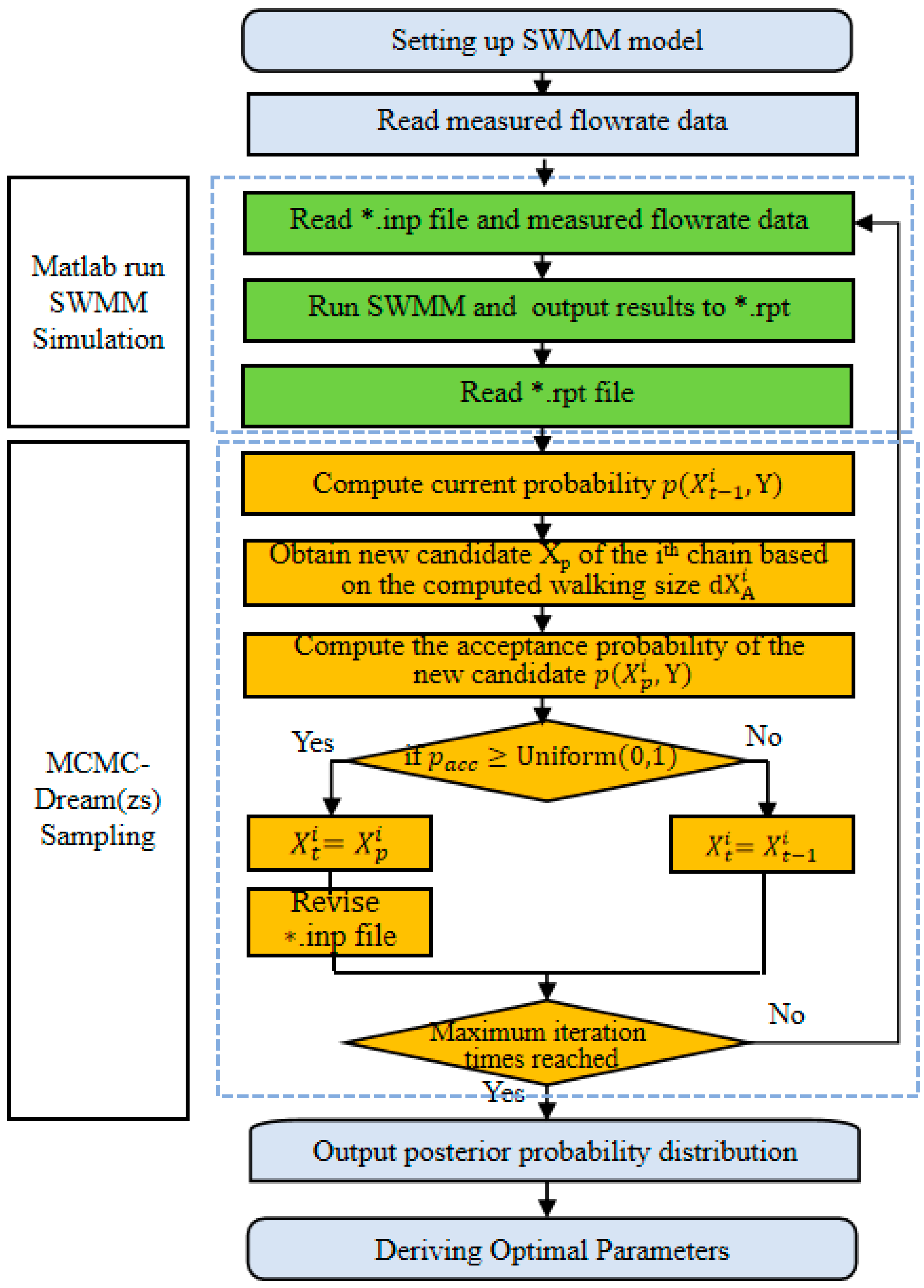
Figure 1. Bayesian DREAM(zs) SWMM calibration framework.
Water 17 03435 g001
Figure 2. Location of study area.
Water 17 03435 g002
Figure 3. Studied rainfall hyetographs. (a) Single-peak. (b) Double-peak. (c) Triple-peak.
Water 17 03435 g003
Figure 4. Coefficient of variance (Cv) of each parameter under rainfall intensities R1–R9.
Water 17 03435 g004
Figure 5. Posterior distribution of parameters under rainfall intensities R1–R9.
Water 17 03435 g005aWater 17 03435 g005b
Figure 6. Posterior distributions of all parameters calibrated using different rainfall patterns. (a) Single-peak rainfall. (b) Double-peak rainfall. (c) Triple-peak rainfall.
Water 17 03435 g006aWater 17 03435 g006b
Figure 7. Boxplots of parameter posterior distributions under three rainfall patterns (S: single-peak rainfall; D: double-peak rainfall; T: triple-peak rainfall).
Water 17 03435 g007
Figure 8. Coefficients of variance (Cv) of parameter posterior distributions for (a) flat terrain watershed (Slope = 0.4%) and (b) steep terrain watershed (Slope = 4%) under three development levels calibrated by five rainfall intensities (rain3–rain7).
Water 17 03435 g008
Figure 9. Standard deviations of (a) flat watersheds and (b) steep watersheds under three levels calibrated for five rainfall intensities (rain3–rain7).
Water 17 03435 g009
Table 1. True values and typical value ranges of parameters.
ParameterImperv
(%)
Width
(m)
Slope
(%)
N-ImpervN-PervS-Imperv (mm)S-Perv (mm)Zero-Imperv (%)
“True” value5050040.010.1250
Value range30–80200–8002–60.005–0.030.05–0.21–32.5–7.50–25
Table 2. Rainfall characteristics of each rainfall event.
Rainfall EventReturn Period (a)Total Rainfall Depth (mm)Description
rain1 (R1)-2.91Low-intensity rainfalls used for urban runoff pollution control purposes
rain2 (R2)0.258.43
rain3 (R3)0.312.94
rain4 (R4)0.525.56
rain5 (R5)142.70Medium-intensity rainfalls used for urban drainage pipe system design purposes
rain6 (R6)259.84
rain7 (R7)582.49
rain8 (R8)1099.62High-intensity rainfalls used for urban flooding control purposes
rain9 (R9)20116.76
Table 3. Six types of watersheds with different hydrological characteristics.
Watershed TypeTwo Types of Terrain FeaturesThree Development Levels
Flat
(Slope = 0.4%)
Steep
(Slope = 4%)
Undeveloped
(20% Impervious)
Medium-Developed
(50% Impervious)
Fully Developed (80% Impervious)
Type IX X
Type II XX
Type IIIX X
Type IV X X
Type VX X
Type VI X X
Table 4. Posterior distribution statistic indexes of each parameter under rainfall R5.
Imperv
(%)
Width
(m)
Slope
(%)
N-ImpervN-PervS-Imperv
(mm)
S-Perv
(mm)
Zero-Imperv (%)
True value5050040.010.1250
Prior distribution range30–80200–8002–60.005–0.030.05–0.21–32.5–7.50–25
Mean value50.095643.2124.3930.0140.1181.9565.4564.316
Standard deviation0.243168.6470.8870.0050.0320.0870.6104.783
Coefficient of variation0.0050.2620.2020.3320.2740.0450.1121.108
Table 5. Standard deviations of parameter posteriors under three rainfall patterns.
Standard Deviation of Parameter Posterior Distribution
Single-PeakDouble-PeakTriple-Peak
Imperv (%)0.2430.2030.310
Width (m)168.647110.789157.441
Slope (%)0.8871.0141.022
N-imperv0.0050.0020.003
N-perv0.0320.0210.042
S-imperv (mm)0.0870.2110.231
S-perv (mm)0.6100.4410.477
Zero-imperv (%)4.7834.44710.047
Disclaimer/Publisher’s Note: The statements, opinions and data contained in all publications are solely those of the individual author(s) and contributor(s) and not of MDPI and/or the editor(s). MDPI and/or the editor(s) disclaim responsibility for any injury to people or property resulting from any ideas, methods, instructions or products referred to in the content.