Excess Rainfall-Based Derivation of Intensity–Duration–Frequency Curves

Abstract

This paper presents an innovative derivation of intensity–duration–frequency (IDF) curves, which play a crucial role in the design of hydraulic infrastructures. IDF curves are herein derived from excess rainfall, that is, the net rainfall obtained by removing abstractions related to hydrological losses from total gross rainfall. When long fine fine-resolution time series of rainfall depth are available at a site, excess rainfall can be obtained by applying a simplified hydrological model of a catchment, including solely the gross-excess rainfall conversion. The application of annual maxima (AM) analysis on excess rainfall intensity data enables the construction of excess rainfall-based intensity–duration–frequency (ERIDF) curves. For assigned rainfall event criticality (return period) and duration, these curves directly provide the associated excess rainfall intensity value. This results in a better preservation of the return period in the rainfall–runoff transformation when used inside the rational formula for estimating peak water discharge, in comparison with the conventional approach adopted by practitioners, based on derivation of IDF curves and on the application of runoff coefficient for gross-excess rainfall conversion inside the rational formula.

1. Introduction

Hydraulic interventions and infrastructures in riverine and urban drainage contexts are conventionally designed by making use of intensity–duration–frequency (IDF) curves [1], which express the relationship between average rainfall intensity and event duration for an assigned event criticality, i.e., probability of exceedance or return period. Depth–duration–frequency (DDF) curves are strictly related to IDF curves, as they describe the event rainfall depth, which can be easily obtained by multiplying average intensity by duration. In the framework of extreme value analysis, two different series are conventionally used for constructing IDF curves, namely the annual maximum (AM) and the peak over threshold (POT) series [2].

In most cases, two- and three-parameter relationships are adopted for IDF curves, consisting of a power law and a power law with time adjustment, respectively. The former expression has the advantage of better simplicity, while the latter features a better fit over a wider range of event durations [3,4,5]. The scientific literature also offers methods to relate the parameters of the three-parameter IDF curves to those of the two-parameter IDF curves, e.g., [6,7], to extend the IDF curves to non-recording rain gauges [8] and to consider spatial aspects associated with the areal extent of rainfall events [9]. Based on an assumption of regularity between the rainfall intensity moments at different event durations, the scale invariance approach was proposed, e.g., see [3], which yields a single mathematical expression to describe the relationship between event intensity and duration at various return periods. This approach was used at both local and regional scales, e.g., [10], and methods to enhance it, e.g., [11], or to expand it to a larger range of event durations, e.g., [3,12], were also proposed. Finally, the impact of climate change on IDF curve parameters was analyzed by other researchers, e.g., [13,14,15,16].

While lots of attention in the scientific literature has been paid to the accurate construction of DDF/IDF curves for assessing rainfall depth/intensity as a function of event duration for an assigned return period in current and future climate scenarios, their integration with initial soil conditions in the design event has been underexplored, though these conditions are well known to play a very important role in rainfall–runoff transformation. In fact, the rainfall depth/average intensity being the same, an initially wet soil results in a larger peak water discharge at the catchment outlet than an initially dry soil. Furthermore, in the conversion from gross to net rainfall, which is performed by applying a multiplicative runoff coefficient on hyetographs constructed based on DDF/IDF curves in most engineering applications, practitioners almost always ignore that this coefficient is not deterministic, as it features its own probability distribution. Indeed, it depends on the event’s total rainfall depth and on initial soil conditions. While the first dependence has been investigated in some contexts, the second has received poor attention from the research community. The choice of a suitable value for this coefficient is indispensable for preserving the level of criticality, i.e., the return period initially assumed in the analysis/design, in the rainfall–runoff transformation. Without a sound statistical treatment of the initial soil conditions in the IDF framework, the only way to obtain a statistically valid peak water discharge estimation is by means of more complex methods, based on generating a long rainfall series converted into a long discharge series using a hydrological model, e.g., [17,18]. To the best of the author’s knowledge, only one attempt to integrate DDF/IDF with initial soil conditions was made in the scientific literature by Creaco [4], who proposed an approach for considering pairs of intense rainfall depths/intensities and initial soil conditions inside a single probabilistic framework. For each return period, the approach of Creaco [4] yields a set of DDF/IDF curves, each of which is associated with a single initial soil condition. The approach proposed by Creaco [4] finds application especially in contexts in which initial soil condition measurements are available at fine temporal resolution, along with those of rainfall intensity. However, a long series of fine-resolution data of initial soil conditions is seldom available, as soil moisture sensors are not so widespread as rain gauges. Furthermore, soil moisture data collected by satellites measuring microwaves have coarse resolution, i.e., a daily time step.

Rather than leaning on initial soil conditions, a more compact and straightforward approach to construct DDF/IDF curves could be applied, which is based on the statistical processing of excess rainfall intensities derived from simplified hydrological modeling. Indeed, this approach has never been explored so far in the scientific literature. The present paper aims to bridge this gap. As excess rainfall intensity condenses the information coming from both rainfall intensity and initial soil conditions, it enables preservation of the return period chosen for the construction of DDF/IDF curves, to be used for peak water discharge estimation.

The remainder of the paper is organized as follows. The following section describes the methodology for the construction of excess rainfall-based intensity duration frequency (ERIDF) curves, followed by its application to two sites, the discussion and the conclusions.

2. Materials and Methods

2.1. Conceptual Overview of the Methodology

The peak water discharge Q (m³/s) in a catchment can be evaluated with the conventional rational method formula [1]:

$$Q={\displaystyle \frac{Ci\left(t_c\right)A}{3.6\times {10}^6}},$$

(1)

in which C (-) and A (m²) are the runoff coefficient, used for gross-excess rainfall conversion, and the catchment area, respectively. Furthermore, i (mm/h) is the rainfall intensity obtained from the IDF curve, as a function of event duration, set equal to catchment concentration time t_c (h). The Formula (1) performs both gross-excess rainfall conversion and rainfall–runoff transformation and holds under the following assumptions:

• Uniform distribution of rainfall over the catchment.
• Constant rainfall intensity for the whole event duration.
• Linear relationship between rainfall and runoff.
• Available storage in the catchment is assumed to be filled, resulting in the absence of storage effects.
• The return period T (years) of the peak discharge rate is the same as the return period of the average rainfall intensity or rainfall event.
• The runoff coefficient C is deterministic and constant for storms of any duration or frequency on the catchment.

The last two assumptions represent a major misconception of many who use the rational formula. Though being conventionally used as a deterministic and constant parameter by practitioners, C indeed depends on rainfall duration and intensity and features its own probability distribution, to be analyzed jointly with the probability distribution of gross rainfall. Therefore, the return period of peak water discharge depends on the return period of both the runoff coefficient and rainfall intensity.

To overcome this methodological flaw, a novel approach is presented in this paper, leaning on the excess, instead of gross, rainfall intensity i_e (mm/h). When i_e is used instead of i (mm/h), the rational Formula (1) takes on the following form, in which C does not appear:

$$Q={\displaystyle \frac{i_e\left(t_c\right)A}{3.6\times {10}^6}}$$

(2)

The presence of i_e in Equation (2) allows taking account of the criticality of both rainfall and soil conditions, within an assigned value of return period T (years). Compared to Equation (1), the advantage of Equation (2) is that the return period T adopted for i_e can be directly transferred to Q.

The derivation of excess rainfall intensity–duration–frequency (ERIDF) curves, which are the main novel contributions of this work, consists of the following two phases, aimed at transforming available long time series of rainfall intensity into series of excess rainfall intensity and at processing them to obtain ERIDF curves, respectively, as is described below.

2.2. Phase 1—Rainfall-Excess Rainfall Conversion

For rainfall-excess rainfall conversion, a simplified hydrologic model based on the application of the long-horizon water balance on a single soil cell is considered. This soil cell is independent of surrounding cells and does not exchange water flows with them. Therefore, the single soil cell is representative of the overall average behavior of the catchment soil.

The following differential equation is solved by means of an explicit first-order numerical method:

$$A{\displaystyle \frac{dl}{dt}}=I\left(t\right)-F\left(t\right)-R\left(t\right),$$

(3)

in which t is the time, in seconds. I, F and R are the rainfall, infiltration and runoff flow patterns in m³/s, respectively. Finally, l (m) is the water level inside the cell. At each time t, I is obtained as follows:

$$I\left(t\right)={\displaystyle \frac{i\left(t\right)\times A}{3.6\times {10}^6}},$$

(4)

in which i(t) is rainfall intensity in mm/h, obtained from long-horizon continuous measurements at the rain gauge.

When it rains (I > 0), F(t) is obtained by means of the Horton infiltration model, while expressing the infiltration capacity f_c (mm/h) as a function of the previously infiltrated rainfall depth F₀, instead of the time along the Horton curve—see the Modified Horton method in [19,20], considering a maximum infiltration capacity f_max (mm/h), a minimum infiltration capacity f_min (mm/h) and a decay constant k (h⁻¹). For the sake of simplicity, R(t) is calculated in such a way that the runoff always empties out the remaining water following the infiltration process inside the generic integration time step. The excess rainfall flow I_e can be calculated by subtracting infiltration from rainfall intensity, as follows:

$$I_e\left(t\right)=I\left(t\right)-F\left(t\right)$$

(5)

When it does not rain (I = 0 and R = 0), the infiltration capacity f is progressively restored by using an exponential drying curve with drying time T_d (days) to simulate the effects of evapotranspiration. The excess rainfall flow I_e is equal to 0.

The differential Equation (3) is solved by adopting the same temporal step as that available in the rain gauge measurements.

By applying this method on long time horizons, e.g., a long series of years, the temporal pattern of excess rainfall intensity i_e(t) is derived as follows:

$$i_e\left(t\right)={\displaystyle \frac{3.6\times {10}^6{I}_e\left(t\right)}{A}}$$

(6)

It must be noted that the simple hydrological modeling described above has reduced computation times, even when applied to long time series. This is because it is performed on a single soil cell without considering the transformation from excess rainfall to runoff and water discharge at the catchment outlet.

It must be noted that the Modified Horton method was chosen in this paper due to its simplicity. Other methods for assessing infiltration can be implemented, e.g., SCS-CN or Green-Ampt. The choice of another method, including potential additional/different parameters, would impact on assessment of F(t) in Equation (5), without altering the remainder of the methodology.

2.3. Phase 2—Construction of Excess Rainfall Intensity–Duration–Frequency (ERIDF) Curves

The traditional annual maximum (AM) approach, which is the most often used for IDF derivation, is based on processing the yearly maxima of rainfall intensity for a given duration. While this approach is conventionally applied on gross rainfall intensity i data, which are extracted from the continuous series of measurements at a certain rain gauge, it is herein applied on excess rainfall intensity i_e data, obtained as was explained in the previous subsection.

The AM approach is based on the following steps:

• Obtaining yearly maxima of rainfall intensity for a certain set of design event durations from a time series.
• Ranking of yearly maxima of rainfall intensity for each design event duration and calculation of the Gumbel cumulative frequency.
• For each duration, the representation of the sample data obtained from step 2 with a maximum value probability distribution [21].
• Considering a single probability of non-exceedance (i.e., return period T) at a time, fitting the IDF curve to the quantiles obtained from step 3 for various event durations.

The step 4 described above results in a mathematical expression expressing the relationship between i_e and t for a fixed value of T, i.e., a single IDF or ERIDF curve for a single value of T. Alternatively, in step 4 the scale invariance approach of Creaco [3], which was initially conceived for gross rainfall data, can be applied on excess rainfall maxima to construct a single mathematical expression to express the dependence of i_e on t and T, i.e., a family of IDF or ERIDF curves. As far as step 4 is concerned, it must be noted that the adoption of a single IDF (or ERIDF) curve for each return period or the alternative use of the scale invariance approach of Creaco [3] have nothing to do with the novelty of the methodology described in the present paper, consisting of the construction of curves based on annual maxima of excess (rather than gross) event intensity.

2.4. Data

The pattern of observed rainfall intensities at two Italian sites, namely Pavia SS35 (Lombardia–Northern Italy) and Erice (Sicily–Southern Italy), made available by the environmental protection agencies of the two Italian regions with a ten-minute resolution in the periods of 2004–2022 and 2003–2021, respectively, was used in this work. No correction was applied to the rainfall data observed at the sub-hourly time resolution.

For the conversion from gross to excess rainfall, two different soils were considered, as shown in the following

Table 1. Soil kind and characteristics.

Soil Kind	fmax (mm/h)	fmin (mm/h)	k (1/h)	Td (days)
1	76	2.5	2	7
2	160	10	2	7

. The soil parameter values were assumed in an attempt to reproduce the behavior of soils with high and moderate–low runoff potential, that is, with low and moderate–high infiltration capacity, associated with Soil Conservation Service groups D and B-C, respectively. Other soil properties than those reported in Table 1, such as saturated/unsaturated zone, moisture conditions, permeability and porosity, were neglected because they do not impact the modified Horton infiltration model described in Section 2.2.

The methodology of this work was implemented in the Matlab^® 2025a environment and applied to the two Italian sites and the two kinds of soil.

3. Results

The model for rainfall-excess rainfall conversion was applied to both case studies and to both kinds of soils considered (Phase 1 of the methodology). In Phase 2 of the methodology, the analysis of time series of gross rainfall intensity i and excess rainfall intensity i_e yielded the yearly maxima of gross and excess rainfall intensity associated with event durations of 10 min, 20 min, 30 min, 40 min, 1 h, 3 h, 6h, 12 h and 24 h reported in the Supplementary Materials (step 1 for construction of IDF and ERIDF curves).

For each site, soil kind (no soil being considered for the construction of conventional IDF curves, and soil 1 and soil 2 for the construction of ERIDF curves), and event duration, the yearly maxima were ranked and assigned a Gumbel cumulative frequency value F (step 2 for the construction of IDF and ERIDF curves). Then, a maximum value probability distribution was fit to the data of step 2 (step 3 for the construction of IDF and ERIDF curves). Based on the results of a preliminary analysis, some of which are reported in Appendix A of the present paper, the Gumbel probability distribution was chosen for step 3. In the cases of gross rainfall intensity or excess rainfall intensity with a soil with moderate infiltration capacity (soil 1), the Gumbel distribution parameters were estimated with the method of moments. 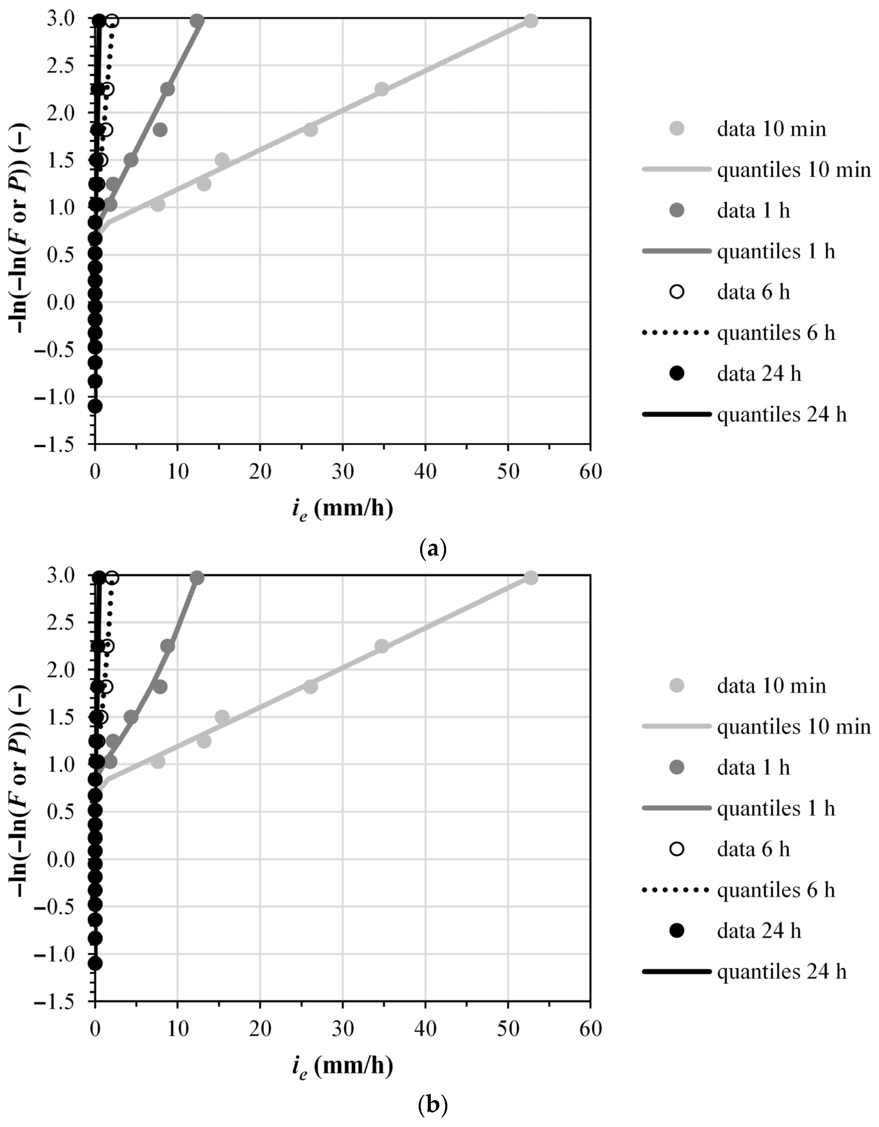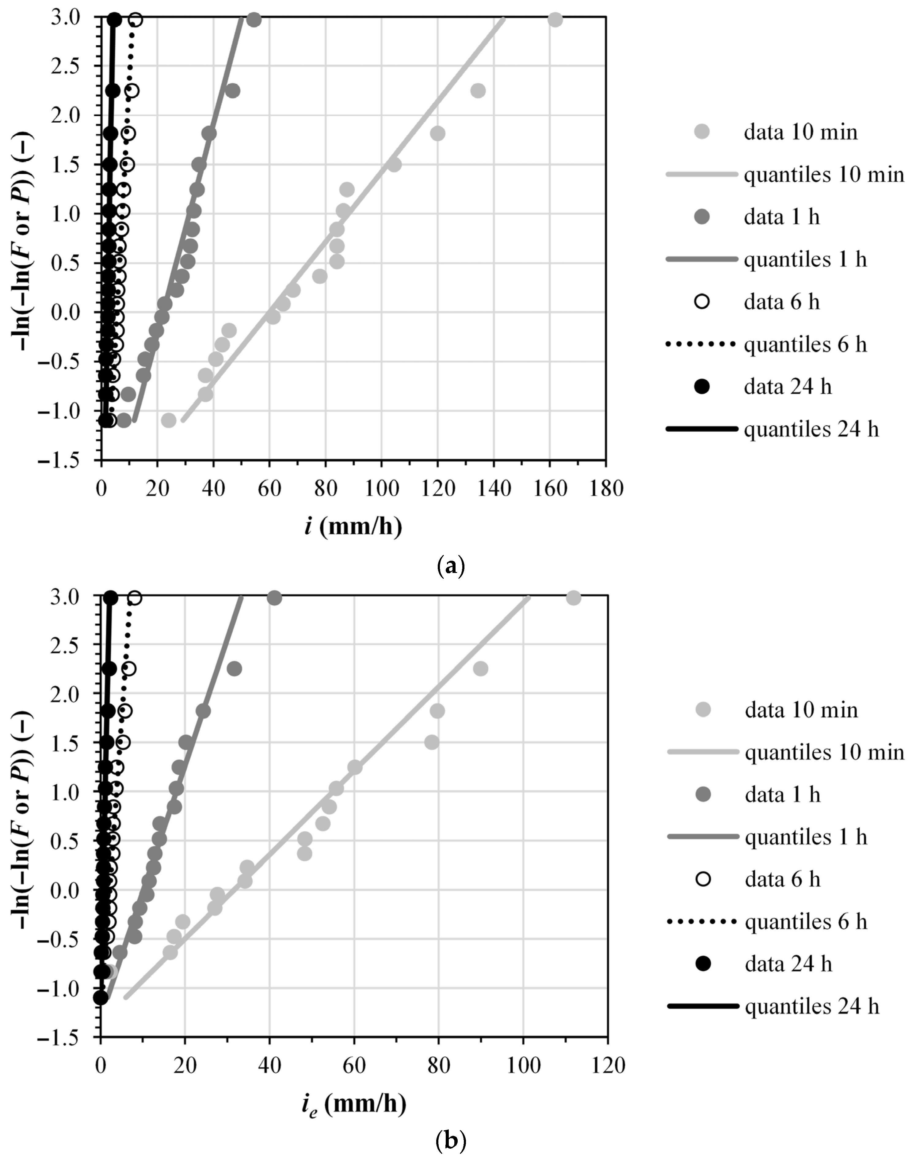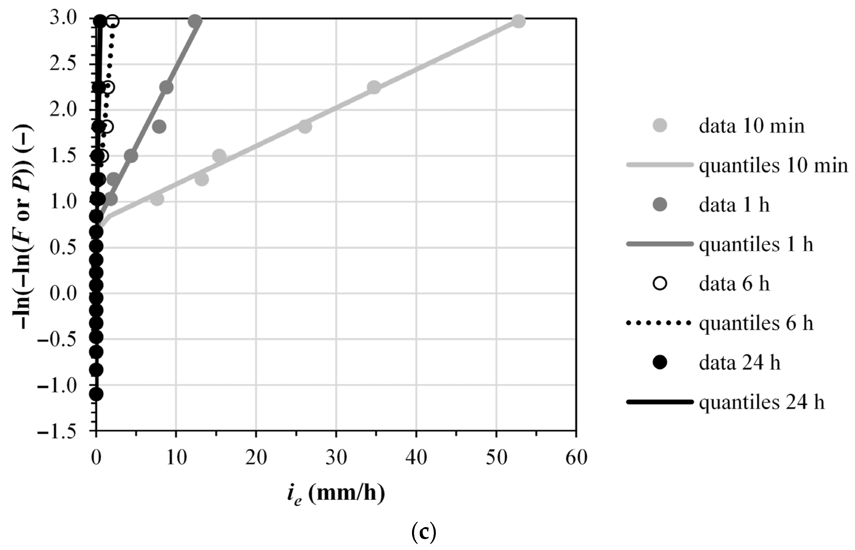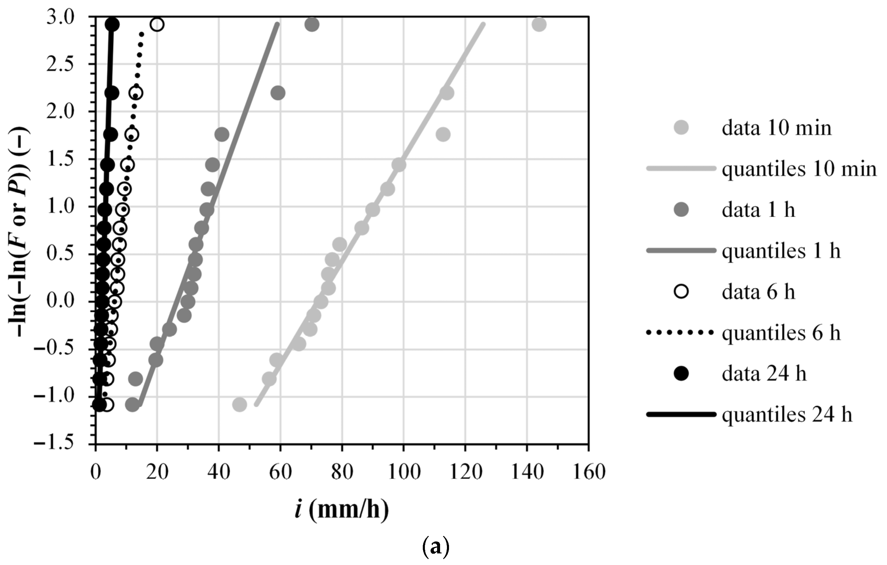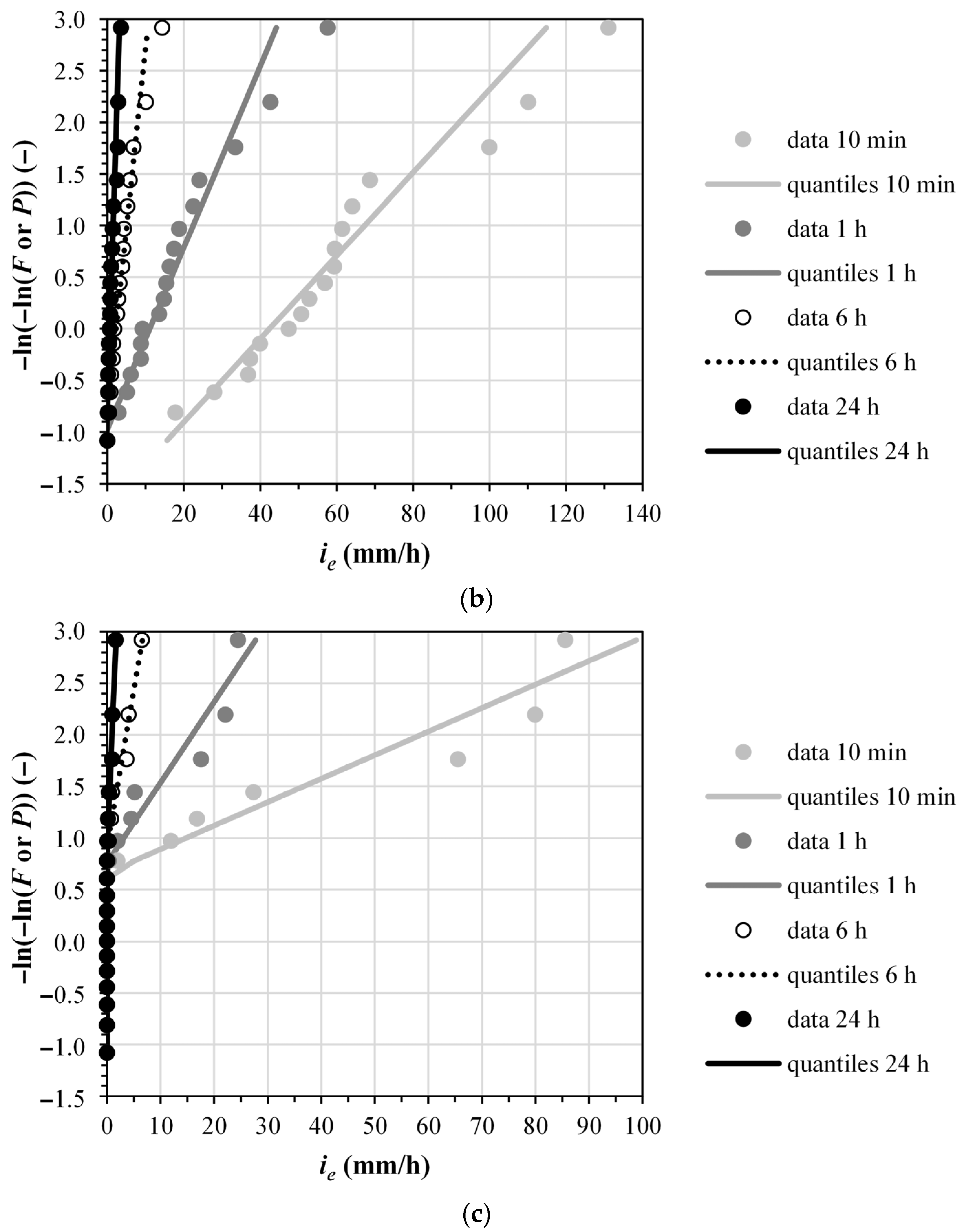In the case of excess rainfall intensity with a soil with high infiltration capacity (soil 2), the parameters estimated with the method of moments required numerical adjustments due to the presence of numerous zeros in i_e data. The comparison of data and Gumbel quantiles for assigned values of cumulative frequency value F/non-exceedance probability distribution P is shown in the following, Figure 1 and Figure 2.

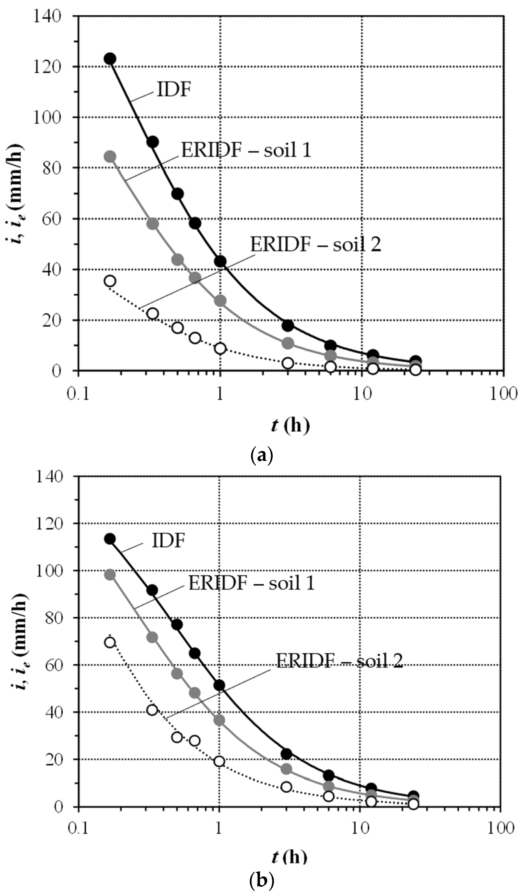
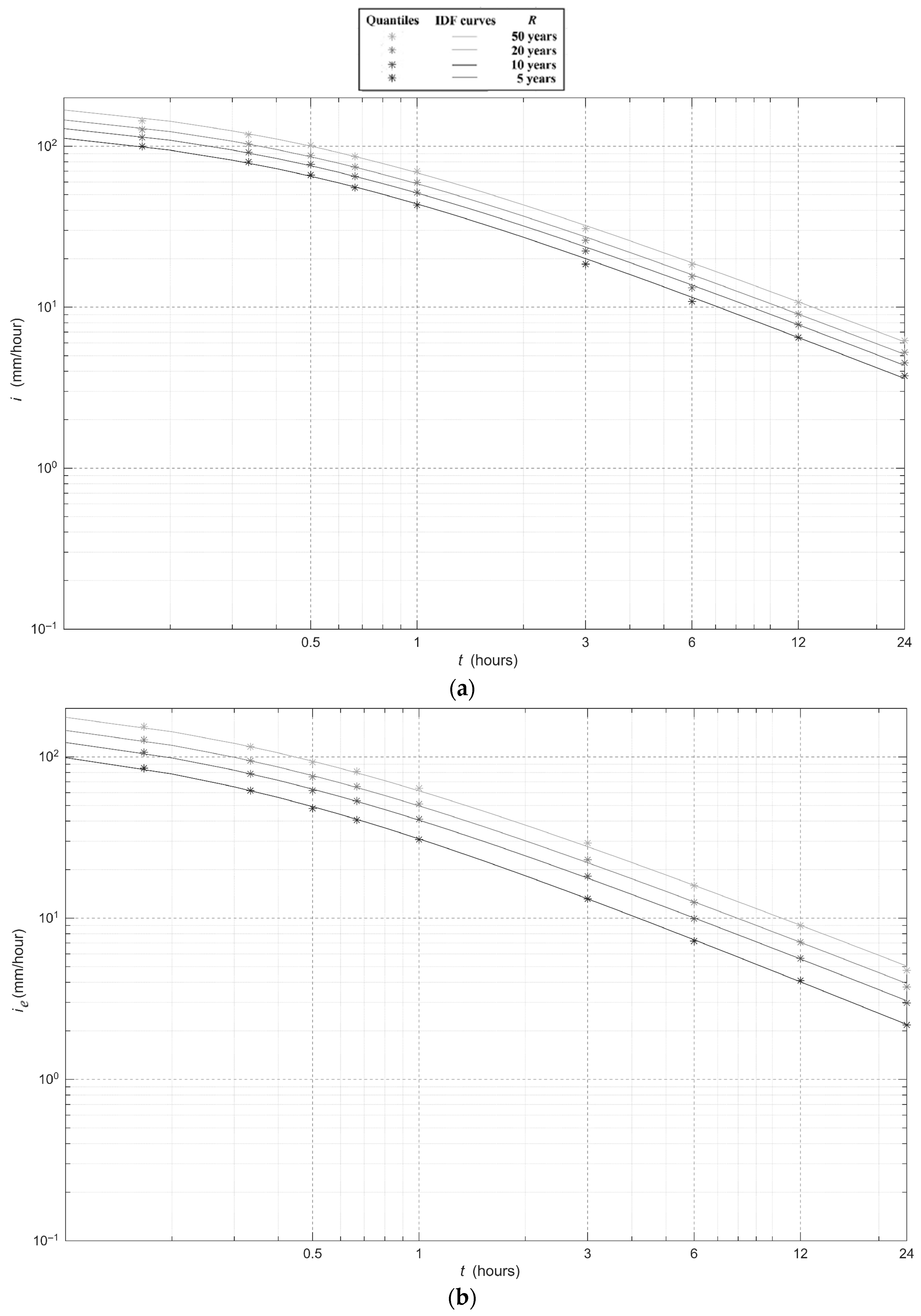
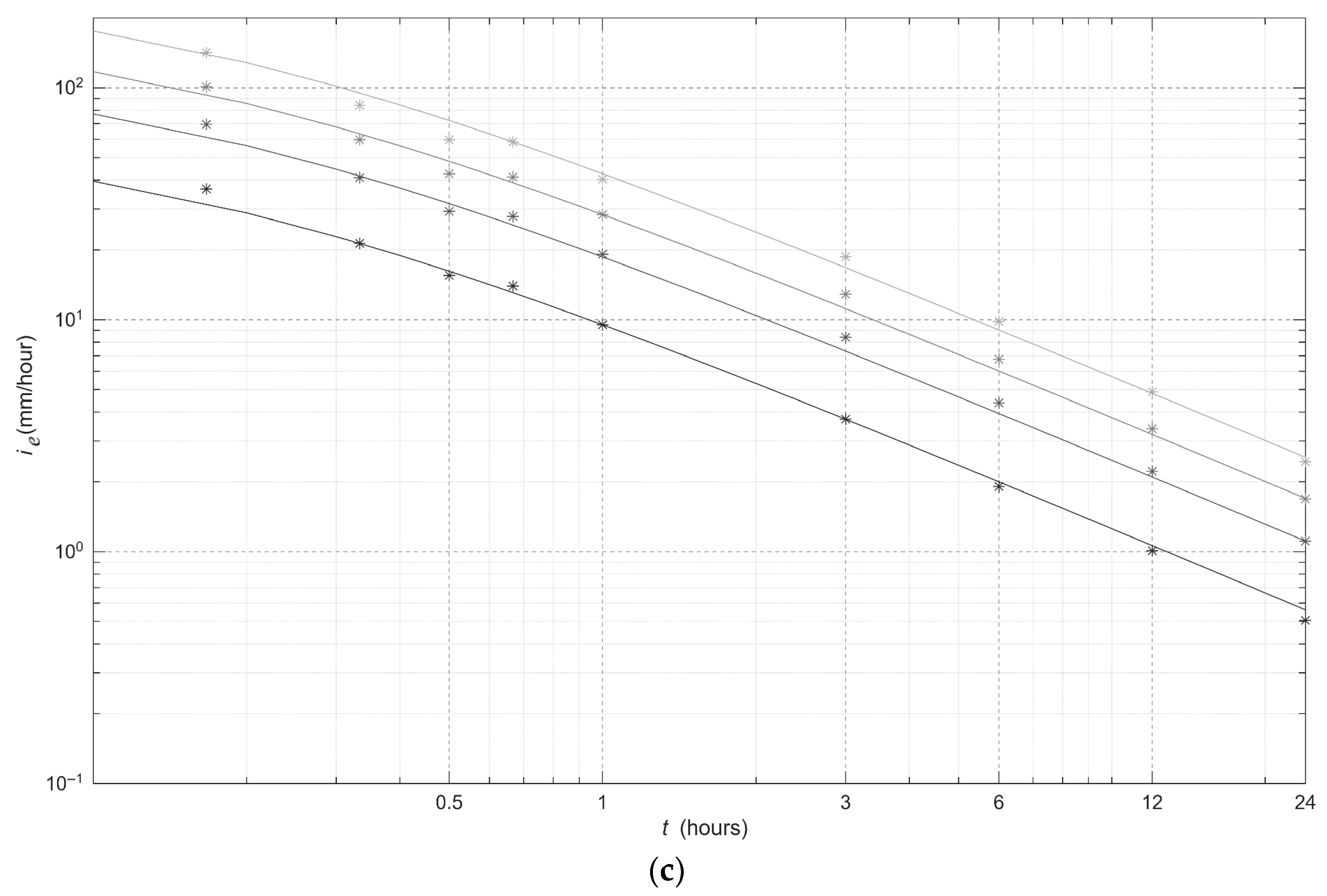
Finally, considering a probability of non-exceedance p = 0.9, i.e., a return period T = 10 years for both case studies, the Gumbel quantiles were obtained for gross rainfall and excess rainfall (soil 1 and soil 2) at all the event durations considered. The best fit of the three-parameter equation $i \mathrm{o}\mathrm{r} i_e=p_1{\left(t+p_3\right)}^{p_2}$ yielded the IDF and ERIDF curves shown in Figure 3 (step 4 of the methodology for IDF/ERIDF construction). The parameter values of these curves are reported in the following

Table 2. Parameters of IDF and ERIDF curves.

Curve	p1	p2	p3
Pavia IDF	49.872	−0.845	0.18
PAVIA ERIDF—soil 1	30.703	−0.905	0.16
PAVIA ERIDF—soil 2	10.540	−1.000	0.16
Erice IDF	68.829	−0.868	0.40
Erice ERIDF—soil 1	43.109	−0.874	0.22
Erice ERIDF—soil 2	18.925	−0.853	0.04

.

Expectedly, the ERIDF curve for soil 1 is lower than the IDF curve, as the rainfall intensities in the ERIDF curve are excess rainfall intensities. The ERIDF curve for soil 2 is lower than the ERIDF curve for soil 1, as soil 2 has a higher infiltration potential than soil 1 (see Table 1). In the case of soils with a larger infiltration potential than soil 2, the resulting ERIDF curves would be lower than the ERIDF curves associated with soil 2 in Figure 3. In the case of soils with a smaller infiltration potential than soil 1, the resulting ERIDF curves would lie between the IDF curve and the ERIDF curve associated with soil 1, tending to the IDF curve when the infiltration potential tends to 0. In this extreme case, F(t) in Equation (5) would always be equal to 0, therefore making excess infiltration I_e equal to gross intensity I.

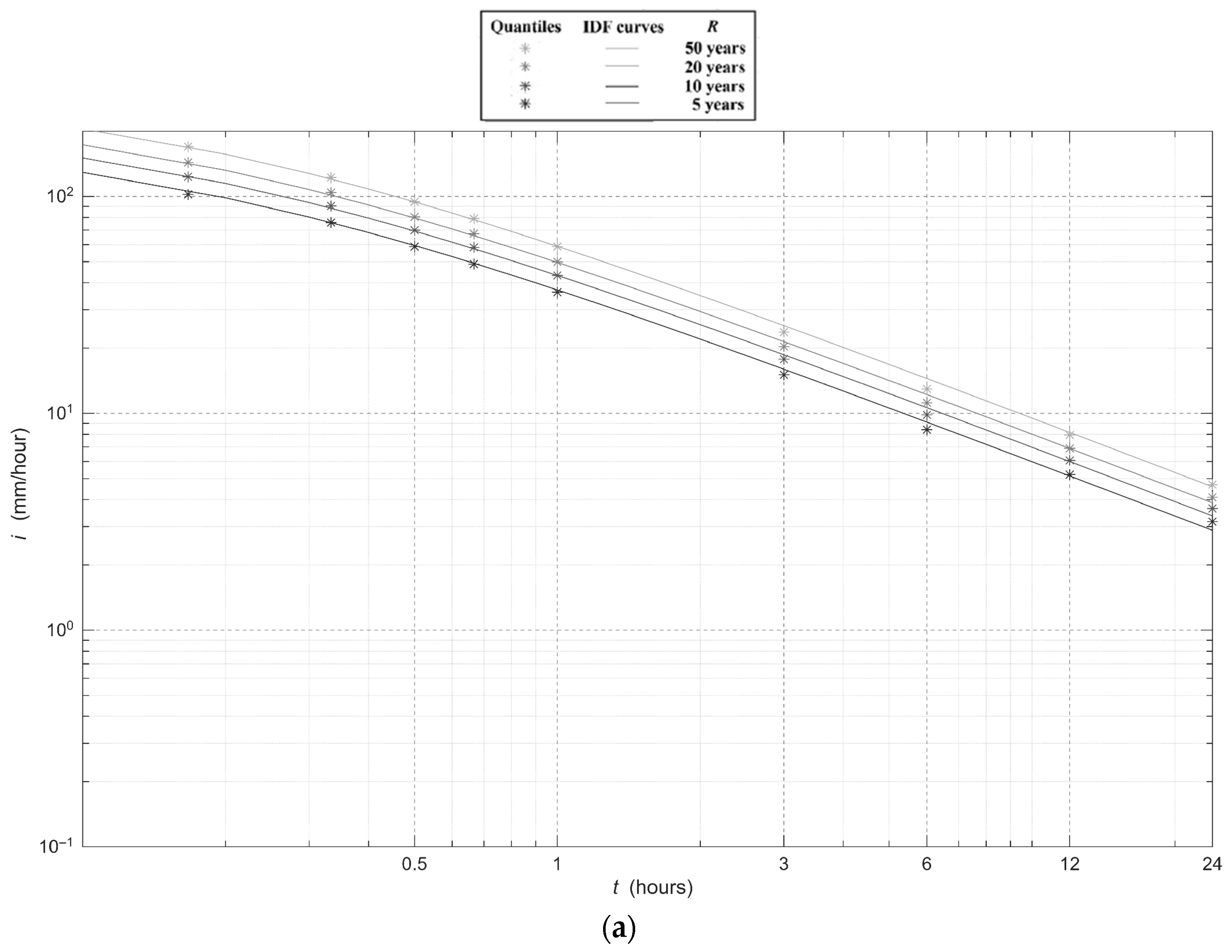
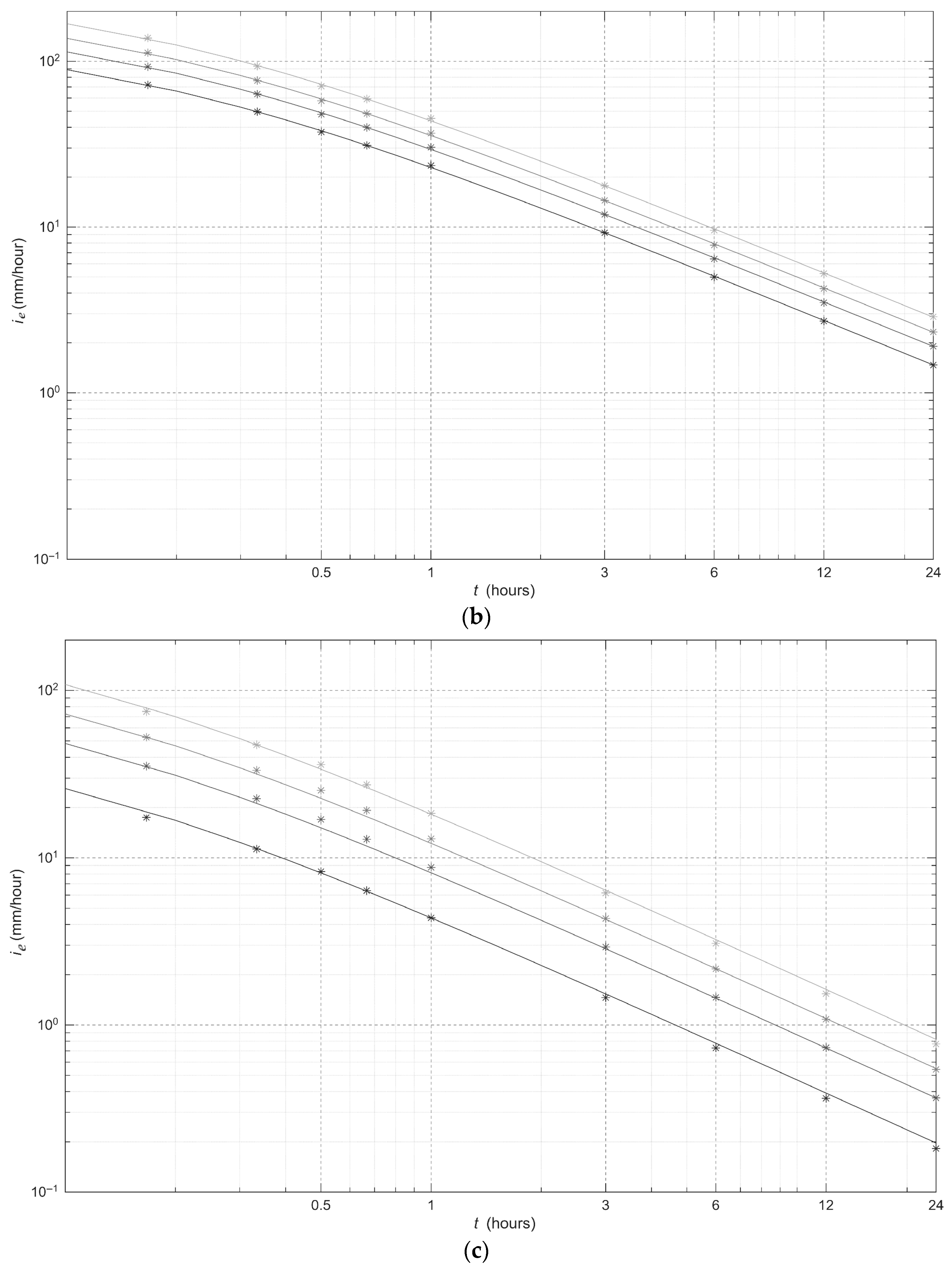
Interestingly, the multiple scaling methodology based on adjusted scale invariance proposed by Creaco [3] can also be applied to rainfall data to obtain, for each site and soil kind, a single equation expressing intensity as a function of duration t at various values of non-exceedance probability P/return period T, like the following:

$$i \mathrm{o}\mathrm{r} i_e=a_1{\left(1+K_P\sqrt{\left(a_2/a_1^2\right){\left(t+c\right)}^{2n\left({\phi }_2-1\right)}-1}\right)\left(t+c\right)}^n,$$

(7)

in which there are eight parameters (namely a₁, a₂, φ₂, c and n plus the three parameters ξ, σ and μ of the frequency factor K_p expressed by means of the Generalized Extreme Value (GEV) distribution [21]. The choice of the GEV distribution for K_p is due to the fact that K_p is estimated based on a large number of data, equal to n_y× n_d, with n_y and n_d being the number of available years for rainfall intensity measurements and n_d the number of event durations considered, respectively, even if n_y is not very extended (see Creaco [3] for more details). The results of this application are reported in Figure 4 and Figure 5 and

Table 3. Results of the parameterization for IDF and ERIDF curves with the methodology of Creaco [3].

Case Study	a1	a2	n	φ2	ξ	σ	μ	c
Pavia IDF	35.206	1371.414	−0.842	1.000	0.121	0.645	−0.460	0.164
Pavia ERIDF—soil 1	16.967	448.226	−0.910	0.993	0.000	0.780	−0.450	0.157
Pavia ERIDF—soil 2	1.000	46.343	−1.000	1.000	0.162	0.595	−0.456	0.082
Erice IDF	46.421	2395.827	−0.884	0.986	0.051	0.726	−0.457	0.354
Erice ERIDF—soil 1	23.540	907.272	−0.960	0.908	0.006	0.774	−0.451	0.222
Erice ERIDF—soil 2	1.000	292.399	−1.000	0.923	0.145	0.617	−0.458	0.148

.

Overall, the results shown in Figure 3, Figure 4 and Figure 5 prove that ERIDF curves fit very well excess rainfall i_e quantiles, in the same way as IDF curves fit gross rainfall i quantiles.

4. Discussion

A straightforward application of ERIDF curves is the evaluation of peak discharge in a catchment. As an example, let us consider a catchment with area A = 100 ha = 1,000,000 m², and a concentration time t_c = 0.278 h situated in the Pavia area. For the return period T = 10 years, the IDF/ERIDF curves $i= \mathrm{o}\mathrm{r} i_e=p_1{\left(t+p_3\right)}^{p_2}$ with the parameters reported in Table 2 can be considered.

In the ERIDF curve framework, the peak water discharge Q (m³/s) can be evaluated with the modified rational method Formula (2), yielding Q = 18.01 m³/s and Q = 7.08 m³/s for soil 1 and soil 2, respectively. The different values of Q are due to the different i_e values, equal to 64.84 mm/h and 25.49 mm/h for the two soils. The gross rainfall being the same, soil 2 infiltrates much more water than soil 1, resulting in a much lower rainfall intensity, with the return period being the same.

If i_e is estimated by means of the multiple scale form (Equation (7)) of Creaco [3] with the parameters in Table 3 and considering soil 2, Equation (2) yields Q = 6.80 m³/s and Q = 15.23 m³/s for T = 10 years and T = 50 years, respectively. To obtain the same results with Equation (1), related to the conventional rational method, two different values of C should be considered, equal to 0.25 and 0.41, for the two values of T, respectively. This means that, as T grows, a decreasing value of C should be considered in the conventional rational method Formula (1) to guarantee preservation of the return period assumed for the design. However, being based on excess rainfall, the approach presented in this paper has the advantage of overcoming the difficulty of defining the suitable value of C for different return periods T.

In the case studies of this paper, a methodology for obtaining the excess rainfall in the simple case of homogeneous soil characteristics inside the catchment is considered. However, the methodology could be generalized to the case of heterogeneous soil characteristics. Furthermore, more complicated and accurate estimations of hydrological losses could be considered without any loss of validity of the approach presented for the derivation of ERIDF curves.

The average excess rainfall intensity obtained from the ERIDF curve can also be used to construct more complex hyetographs than the rectangular hyetograph assumed in the rational method. These hyetographs can be used in the context of event hydrological modeling for the construction of the whole hydrograph, rather than just peak water discharge estimation.

5. Conclusions

A novel methodology was developed in the present work for the construction of the ERIDF curves, namely IDF curves based on excess rainfall instead of gross rainfall.

The main conclusions of this work are the following:

• Excess rainfall time series were derived by applying a simple hydrological model to a long-horizon time series of gross rainfall.
• The annual maxima of excess rainfall intensity were statistically analyzed at various event durations and represented with extreme value distributions, like the Gumbel.
• Three-parameter IDF curves and IDF curves based on scale invariance were constructed for excess rainfall intensity.
• ERIDF curves were proven to yield a sounder evaluation of the peak water discharge at the exit of a hydrological catchment by implicitly considering the probability distribution of both rainfall intensity and runoff coefficient.

As the present work focused on an indirect estimation of excess rainfall based on the coupled use of gross rainfall measurements and of a simple hydrological model for gross-excess rainfall conversion, future developments will be aimed at conceiving methods for deriving direct excess rainfall estimates, e.g., by means of satellite data on rainfall and soil moisture.