Article

Spatiotemporal Changes in Grassland Yield and Driving Factors in the Kherlen River Basin (2000–2024): Insights from CASA Modeling and Geodetector Analysis

1
College of Geomatics, Xi’an University of Science and Technology, Xi’an 710054, China
2
State Key Laboratory of Resources and Environmental Information System, Institute of Geographic Sciences and Natural Resources Research, Chinese Academy of Sciences, Beijing 100101, China
3
Xi’an Mineral Resources Investigation Centre of the China Geological Survey, Xi’an 710100, China
4
Qinling—Loess Plateau Transition Zone Observation and Research Station for Coupling of Soil and Water Elements and Conservation of Biological Resources, Weinan 714300, China
*
Author to whom correspondence should be addressed.
Water 2025, 17(23), 3397; https://doi.org/10.3390/w17233397
Submission received: 22 October 2025 / Revised: 22 November 2025 / Accepted: 25 November 2025 / Published: 28 November 2025

Abstract

The Kherlen River Basin is a typical basin in the eastern Mongolian Plateau and is dominated by grassland. This study estimated the grassland yield in the Kherlen River Basin using the Carnegie–Ames–Stanford approach (CASA) model, combined with Theil–Sen median trend analysis and the Geodetector, to explore its spatiotemporal changes and driving factors. This integrated framework links temporal trend detection with spatial interaction analysis to better reveal ecological responses to climatic and anthropogenic influences. The results showed the following: (1) The root mean square error (RMSE) between the estimated grassland yield and the laboratory measurements was 37.88 g/m2, with an estimation accuracy (EA) of 73.52%. (2) From 2000 to 2024, the grassland yield increased significantly at a rate of 1.98 g/(m2·a) (p < 0.05), with the fastest growth in the middle reaches. (3) Spatially, 79.78% of the basin exhibited significant increases, mainly in the central and western regions. The proportion of significant increase was highest in the upper reaches (40.36%), followed by the middle (32.89%) and lower reaches (6.53%). (4) Due to limited temporal resolution of socioeconomic data, the driving factor analysis covered the period 2000–2020, during which the overall grassland yield was primarily influenced by the interaction between precipitation and elevation (q = 0.6371). Specifically, the upper, middle, and lower reaches were mainly influenced by the interactions between temperature and precipitation (q = 0.6772), precipitation and elevation (q = 0.6377), and temperature and elevation (q = 0.4255), respectively. The study indicates that grassland yield in the Kherlen River Basin exhibited an overall increasing trend during 2000–2024, with climatic factors (precipitation and temperature) and the geographic factor (elevation) identified as the dominant drivers. The influence of human activities was not significant, although this result may be affected by uncertainties associated with data resolution limitations. Future work should incorporate higher-resolution remote sensing and socioeconomic datasets to better assess the impacts of human activities.

1. Introduction

Grassland ecosystems represent the dominant component of terrestrial ecosystems and play a crucial role in the material cycles and energy flow in the atmosphere, hydrosphere, and biosphere [1,2,3]. Owing to the joint effects of environmental change and human intervention, grassland, as the essential material foundation supporting pastoral livestock production, has continuously decreased in extent and degraded in quality [4,5,6]. The continuous degradation of grassland productivity and the ongoing expansion of desertification have become major constraints on grassland ecosystem stability and the sustainable development of regional society and economy [7,8]. Consequently, assessing grassland ecosystem productivity and analyzing its influencing factors are essential for providing a scientific basis for grassland ecosystem conservation and restoration.
Grassland yield (GY) represents the biomass accumulated per unit grassland area over a specified time period and is widely used as a key metric for assessing grassland productivity and grazing capacity. The main approaches to estimating grassland yield include field sampling and remote sensing-based modeling using vegetation indices [9,10]. Although field quadrat sampling provides accurate measurements of grassland yield, this approach is labor-intensive, time-consuming, and unsuitable for large-scale, long-term monitoring. In contrast, remote sensing technology has been widely applied due to its advantages of broad spatial coverage, long temporal records, and rapid data acquisition. There are three main approaches for estimating grassland yield using remote sensing technology: the empirical method, the physical model method, and the net primary productivity (NPP) conversion method [11]. The empirical method estimates grassland yield by establishing linear or nonlinear relationships between vegetation indices and field-sampled data [12]. Although this method is simple to apply, its reliance on ground sampling data and lack of consideration for environmental variables result in poor transferability across regions [13]. The physical model method estimates grassland yield based on mathematical formulations and physical principles. At present, the most commonly used physical model for grassland yield estimation is the radiative transfer model [14]. This model does not require field sampling data and is entirely grounded in physical mechanisms, offering strong parameter interpretability. However, its complex structure and high sensitivity to input parameter accuracy impose certain limitations on its practical application [15]. The NPP conversion method is primarily represented by the Carnegie–Ames–Stanford Approach (CASA) model. By integrating regional environmental characteristics with vegetation-specific light use efficiency parameters, the CASA model enables accurate large-scale estimation of grassland biomass [16]. Some scholars have utilized Moderate Resolution Imaging Spectroradiometer (MODIS) Normalized Difference Vegetation Index (NDVI) data in conjunction with the CASA model to simulate vegetation productivity across the Mongolian Plateau from 2000 to 2019, and to quantify the effects of various driving factors on its spatial distribution and temporal variations [17]. Other researchers used GIMMS (Geophysical Institute Multi-Sensor Spectral Reflectance Database) NDVI data to estimate vegetation productivity in Mongolia for the period 1982–2011 by applying the CASA model and further examined its temporal evolution and climatic responses [18]. In addition, a study employed a modified CASA model to retrieve the net primary productivity of grasslands in Zhenglan Banner, Inner Mongolia, and to estimate the corresponding grassland yield [19]. Another study, based on surface reflectance data, developed aboveground biomass and carrying capacity models grounded in the CASA framework, and evaluated the grassland carrying capacity of Mongolia during the winter–spring period [20]. Therefore, the CASA model offers clear advantages for large-scale grassland yield estimation in regions where field sampling is limited and has consequently been widely adopted in related studies. Regarding the driving factors of grassland yield variation, current research has primarily focused on the impacts of climate change, while comparatively fewer studies have addressed the effects of human activities [21]. Previous studies have separated the effects of human activities on vegetation change using the residual analysis method; however, the simplicity of this approach imposes certain limitations on its accuracy and prevents it from capturing the interactions between natural and anthropogenic factors [22]. The Geodetector model is a statistical framework designed to quantify spatial heterogeneity in geographic phenomena and to identify the factors that drive such patterns. It is primarily applied to explore the spatial distribution patterns of geographical elements, identify influencing factors and their interactions, and is characterized by advantages such as nonlinearity and interpretability [23]. Some researchers have used the Geodetector model to analyze the effects of natural and human factors on the Normalized Difference Vegetation Index (NDVI) in the Kherlen River Basin and have concluded that temperature and precipitation are the dominant factors influencing the variation in the NDVI in the basin [24]. Other scholars have employed residual analysis and the Geodetector model to investigate the driving factors behind vegetation changes and their spatial distribution in the inland river basins of the Hexi Corridor [25]. Therefore, for the Kherlen River Basin, a typical transboundary basin characterized by limited available sample data, the CASA model represents the most suitable approach for estimating grassland yield at regional spatiotemporal scales. To comprehensively investigate how the interactions among climatic, anthropogenic, and topographic factors drive regional grassland productivity, this study employed the Geodetector model as the analytical framework for identifying driving forces. This integrated CASA-Geodetector framework enables a holistic analysis of spatiotemporal dynamics and driving factors across river reaches.
As a typical basin in the eastern Mongolian Plateau, the Kherlen River Basin holds significant importance within the transboundary pastoral system of Mongolia and China [26]. Existing studies on grassland yield in the Kherlen River Basin are primarily focused on comparative analyses of grassland dynamics and their driving factors between the two countries. For example, using a grassland dynamics model and correlation analysis, some scholars have revealed that grassland changes in the basin during 1980–2020 were jointly influenced by natural and anthropogenic factors, with a decrease observed in Mongolia and an increase in China [27]. However, little research has focused on grassland yield across different reaches of the Kherlen River Basin. In this study, grassland yield from 2000 to 2024 was estimated based on MODIS NDVI data combined with the CASA model. In addition, we employed the Theil–Sen median trend method together with the Geodetector model to characterize the spatiotemporal dynamics of grassland yield and to identify its dominant drivers, thereby offering robust scientific support for ecological restoration and sustainable grassland management in the Kherlen River Basin.

2. Materials and Methods

2.1. Study Area

The Kherlen River rises on the southern flank of Mongolia’s Khentii Mountains, flows west to east across Mongolia and China, and eventually pours into Hulun Lake in Inner Mongolia, China (Figure 1). The Kherlen River Basin (107.5° E–117.5° E, 46.5° N–49.5° N) lies at an elevation ranging from 531 to 2511 m, with a west–high, east–low topography dominated by low mountains and hills. Grassland is the predominant vegetation type. The area experiences a temperate continental climate, with long-term mean annual temperatures ranging from 0 °C to 3.2 °C and annual precipitation varying between 156.2 mm and 270.6 mm. The Kherlen River has a total length of 1264 km and drains an area of 23.86 × 10⁴ km2. Based on topographic features, the basin is divided into upper, middle, and lower reaches. The upper reaches cover 12.70 × 10⁴ km2 (53.23% of the basin area), with mountainous terrain on both sides and elevations mostly above 1000 m; the middle reaches cover 7.99 × 10⁴ km2 (33.48% of the basin area), with elevations mainly between 700 m and 1000 m; and the lower reaches cover 3.17 × 10⁴ km2 (13.29% of the basin area), where elevations are generally below 700 m. The China–Mongolia border is located within the lower reach, where the Chinese section extends 206.44 km with a drainage area of 2.97 × 10⁴ km2.

2.2. Data and Processing

The datasets used in this study included (Table 1) the following: (1) Digital elevation model (DEM) data, represented by the 30 m resolution ASTER GDEM V3, obtained from the Geospatial Data Cloud platform (https://www.gscloud.cn). Based on the DEM data, the watershed boundary and river network of the Kherlen River Basin were derived using the hydrological analysis module in ArcGIS 10.8.1(Figure 1). (2) Remote sensing data, consisting of 250 m resolution 16-day MOD13Q1 NDVI products from 2000 to 2024, downloaded from the National Aeronautics and Space Administration (NASA) (https://lpdaac.usgs.gov/) in HDF-EOS format. The data were converted using MATLAB R2024b, and monthly values were calculated by averaging. (3) Meteorological data, including monthly mean temperature, cumulative precipitation, and total solar radiation at 0.1° spatial resolution from 2000 to 2024, obtained from the Copernicus Climate Data Store (https://www.copernicus.eu/en) in NetCDF format. The datasets were decompressed with MATLAB to obtain monthly values, and annual temperature and precipitation were derived using mean value and cumulative synthesis methods, respectively, to analyze the driving factors of grassland yield dynamics. (4) Land-use data, represented by the annual MCD12Q1 land cover product with a spatial resolution of 500 m from 2000 to 2024, downloaded from the National Aeronautics and Space Administration (NASA) (https://lpdaac.usgs.gov/) in HDF-EOS format. The data were converted to annual values using MATLAB. (5) Livestock data, obtained from the statistical yearbooks of China and Mongolia (http://tj.nmg.gov.cn/ and http://www.1212.mn/). Spatial interpolation of annual livestock numbers during 2000–2020 was conducted using the inverse distance weighting (IDW) method, generating raster data with a spatial resolution of 250 m. (6) Human population (People) data, consisting of annual population datasets with a spatial resolution of 1 km from 2000 to 2020, downloaded from the LandScan platform (https://www.ornl.gov/). (7) Gross domestic product (GDP) data, represented by annual GDP datasets with a spatial resolution of 9 km from 2000 to 2020, obtained from https://www.nature.com/articles/s41597-025-04487-x#Sec12 (accessed on 15 June 2025) [28].
The above datasets were projected and resampled to a spatial resolution of 250 m to match the NDVI data using ArcGIS. Specifically, the land-use data were resampled using the nearest-neighbor method, while the DEM, meteorological, population, and GDP data were resampled using bilinear interpolation. The datasets were then clipped to the boundary of the Kherlen River Basin. As a result, we obtained monthly 250 m resolution datasets of MODIS NDVI, mean temperature, precipitation, and total solar radiation for 2000–2024; annual 250 m resolution land-use data for 2000–2024; and annual 250 m resolution datasets of mean temperature, precipitation, livestock numbers, population, GDP, and DEM data for 2000–2020. In addition, slope data were derived from the DEM.

2.3. Methods

2.3.1. CASA Model

The CASA model is a typical light use efficiency model that simulates vegetation net primary production (NPP) at a monthly scale based on the absorbed photosynthetically active radiation and the light use efficiency [29]. In this study, an improved CASA model was employed to estimate grassland NPP in the Kherlen River Basin, with the calculation formula expressed as follows [30]:
NPP x , t = APAR x , t × ε x , t
where NPP (x, t) denotes the net primary production at pixel x in month t; APAR (x, t) represents the absorbed photosynthetically active radiation (MJ/m2) at pixel x in month t; and ε (x, t) indicates the actual light use efficiency (gC/MJ) at pixel x in month t.
The absorbed photosynthetically active radiation (APAR) is governed by incoming solar radiation together with land cover properties, and its computation is expressed as follows:
APAR x , t = SOL x , t × FPAR x , t × 0.5
where SOL (x, t) is the total solar radiation (MJ/m2) at pixel x in month t; FPAR (x, t) is the fraction of incident photosynthetically active radiation (PAR) absorbed by the land cover; and the constant 0.5 represents the proportion of incident PAR available to the land cover relative to the total solar radiation.
The fraction of absorbed photosynthetically active radiation (FPAR) shows a strong linear association with vegetation indices such as NDVI and the simple ratio (SR). By integrating these two approaches, FPAR was estimated using the following equation:
FPAR NDVI x , t = NDVI x , t NDVI i , min NDVI i , max NDVI i , min × FPAR max FPAR min + FPAR min
FPAR S R x , t = 1 + N D V I x , t 1 N D V I x , t S R i , min S R i , max S R i , min × F P A R max F P A R min + F P A R min
F P A R x , t = a F P A R N D V I x , t + 1 a F P A R S R x , t
where FPARNDVI (x, t) represents the NDVI-derived estimate of absorbed photosynthetically active radiation for pixel x during month t; NDVI (x, t) is the NDVI value at pixel x in month t; NDVIi,max and NDVIi,min represent the maximum and minimum NDVI values of land-use type i, respectively (Table 2); FPARmax and FPARmin are constants independent of land-use type, set to 0.950 and 0.001, respectively; FPARSR (x, t) represents the SR-based estimation of absorbed photosynthetically active radiation for pixel x in month t; SRi,max and SRi,min are the 95th and 5th percentiles of SR for land-use type i, respectively (Table 2); FPAR (x, t) is the fraction of absorbed photosynthetically active radiation at pixel x in month t; and a is an adjustment coefficient between the two methods, with a fixed value of 0.5.
The light use efficiency (ε) is primarily determined by temperature and moisture, and its calculation is expressed as follows:
ε x , t = T ε 1 x , t × T ε 2 x , t × W ε x , t × ε max
T ε 1 x , t = 0.80 + 0.02 × T o p t x 0.0005 × T o p t x 2
T ε 2 x , t = 1.1814 1 + exp 0.2 × T o p t x 10 T x , t × 1 1 + exp 0.3 × T o p t x 10 + T ( x , t )
In the equation, Tε1 (x, t) and Tε2 (x, t) represent the low-temperature and high-temperature stress effects on light use efficiency, respectively; Wε (x, t) denotes the moisture stress effect on light use efficiency; εmax is the maximum light use efficiency under optimal conditions, with different constants assigned to different land-use types; Topt (x) refers to the mean temperature in the month when the NDVI of a given region reaches its annual maximum; and T (x, t) is the mean temperature of pixel x in month t.
The εmax values differ across land-use categories. In this study, the εmax parameters for the Kherlen River Basin were derived from simulations conducted with the BIOME-BGC ecological–physiological process model. Specifically, εmax was set as follows: 1.008 gC/MJ for evergreen needleleaf forest, 1.103 gC/MJ for deciduous coniferous forest, 1.044 gC/MJ for deciduous broadleaf woodland, 1.116 gC/MJ for mixed forest, 0.768 gC/MJ for sparse forest, 0.888 gC/MJ for shrubland, 0.608 gC/MJ for grassland, 0.604 gC/MJ for cropland, and 0.389 gC/MJ for urban area, water body, gravel land, and wetland [30].
The moisture stress coefficient Wε (x, t) reflects the influence of available water conditions on light use efficiency, and its calculation is given as follows:
W ε x , t = 0.5 + 0.5 × E x , t E p x , t
E x , t = P x , t × R n x , t × P x , t 2 + R n x , t 2 + P x , t × R n x , t P x , t + R n x , t × P x , t 2 + R n x , t 2
E p x , t = E x , t + E p 0 x , t 2
In the equation, E (x, t) denotes the actual evapotranspiration of pixel x in month t; Ep (x, t) represents the potential evapotranspiration of pixel x in month t; P (x, t) is the cumulative precipitation of pixel x in month t; Rn (x, t) indicates the net solar radiation of pixel x in month t; and Ep0 (x, t) refers to the local potential evapotranspiration, calculated using the method from the vegetation–climate relationship model proposed by Thornthwaite [32].

2.3.2. Grassland Yield Estimation Model

The grassland yield per unit area is derived from vegetation NPP, and its calculation is expressed as follows:
Y n = N P P t 1 + r
In the equation, Yn represents the grassland yield per unit area (g/m2). The coefficient r represents the biomass ratio between the belowground and aboveground components of grassland vegetation. As no relevant measurements are currently available for the study area, this study adopted parameter values reported for ecologically similar regions with comparable grassland types and further refined the ratio accordingly. The r values for different grassland types were set as follows: the values were 5.26 for temperate meadow steppe, 4.25 for temperate steppe, and 7.89 for both temperate desert steppe and temperate desert [33]. The parameter t, which converts biomass into productivity, was treated as a constant with a value of 0.45 [34].

2.3.3. Accuracy Validation

Based on field quadrat data, the estimation results of grassland yield were validated using two indicators, root mean square error (RMSE) and estimation accuracy (EA). The calculation formulas are as follows:
R M S E = i = 1 i = n Y i Y i 2 N × 100 %
E A = 1 R M S E Y ¯ × 100 %
In the equation, Yi and Yi′ denote the measured and estimated values of grassland yield, respectively; Y ¯ represents the mean of the measured grassland yield; and N is the total number of observed samples of grassland yield.

2.3.4. Trend Analysis

The Theil–Sen median trend method was employed to analyze the variation trends of grassland yield in the Kherlen River Basin during 2000–2024. This method has the advantage that the data are not required to follow a normal distribution, and it can reduce the interference of outliers, thereby effectively minimizing the influence of measurement errors or anomalous data [35]. The computation is expressed as follows:
β = Median x i x j i j 1 i j n
In the formula, β denotes the trend slope, representing the variation trend of grassland yield during the study period; Median refers to the median function; n denotes the time-series span, which in this study is 25; i and j are temporal indices indicating different years within the study period; and xi and xj represent the grassland yield values corresponding to year i and year j, respectively. A positive β (>0) indicates an increasing trend in grassland yield during the study period, whereas a negative β (<0) reflects a declining tendency. The statistical significance of the identified trend was subsequently assessed using the Mann–Kendall test, and the corresponding calculation formula is presented below:
Z = S V a r S S > 0 0 S = 0 S + 1 V a r S S < 0
When the absolute value of Z exceeds 1.96, the trend is considered statistically significant at the 95% confidence level. In this study, four types of variation trends were identified: significant increase, non-significant increase, significant decrease, and non-significant decrease.

2.3.5. Geodetector Model

The Geodetector is a statistical tool designed to analyze the spatial heterogeneity of geographical phenomena and to reveal the interactions among variables. It encompasses four core functions: factor detector, interaction detector, ecological detector, and risk detector [36]. In this study, owing to the limited temporal resolution of the socioeconomic data, we harmonized all datasets to a uniform time span of 2000–2020 to quantify the driving effects of various factors on grassland productivity in the Kherlen River Basin. A grid with 100 rows and 100 columns was generated based on the spatial extent of the study region, and the pixel values were extracted into the grid. A total of 3956 valid samples were obtained within the study area, and after removing invalid values, 3422 effective sampling points were retained for analysis. To minimize the total variance within each class, and following common practices in similar studies, the natural breaks (Jenks) classification method was applied in this study to divide the driving factors into six categories [24,37]. Subsequently, the factor detector, interaction detector, and ecological detector modules of the Geodetector were employed to identify the dominant driving factors influencing variations in grassland yield and to quantify their explanatory power. Among them, factor detectors are primarily aimed at quantifying the explanatory power of each independent variable on the spatial heterogeneity of the dependent variable, expressed by the q statistic. A larger q value reflects a greater ability of the independent variable to account for variations in the dependent variable [38].
q = 1 h = 1 L N h σ h 2 N σ 2
In the formula, q represents the explanatory power of the driving factor, with values ranging from [0, 1]; a larger q indicates a stronger influence of the factor. L denotes the number of categories of the variable; N and Nh represent the total sample size of the study area and the sample size of category h, respectively; and σh2 and σ2 refer to the variance within category h and the variance of the entire study area, respectively.
The interaction detector is used to analyze the interactive effects between different factors, that is, to evaluate whether the interaction between any two factors (e.g., X1 and X2) weakens or strengthens their influence on the dependent variable Y, or whether they act independently in affecting Y [39] (Table 3).
The core of the ecological detector lies in comparing whether there is a significant difference in the effects of two factors (e.g., X1 and X2) on the spatial distribution pattern of the dependent variable Y, with the significance of the difference tested using the F statistic:
F = N X 1 N X 2 1 S S W X 1 N X 2 N X 1 1 S S W X 2
In the formula, NX1 and NX2 denote the sample sizes of factors X1 and X2, respectively; SSWX1 and SSWX2 represent the sum of within-stratum variances formed by X1 and X2, respectively. The null hypothesis is as follows:
H 0 : S S W X 1 = S S W X 2
If the null hypothesis is rejected, it indicates that factors X1 and X2 exert significantly different effects on the spatial distribution of the dependent variable Y.

3. Results

3.1. Validation of Grassland Yield Estimation Results

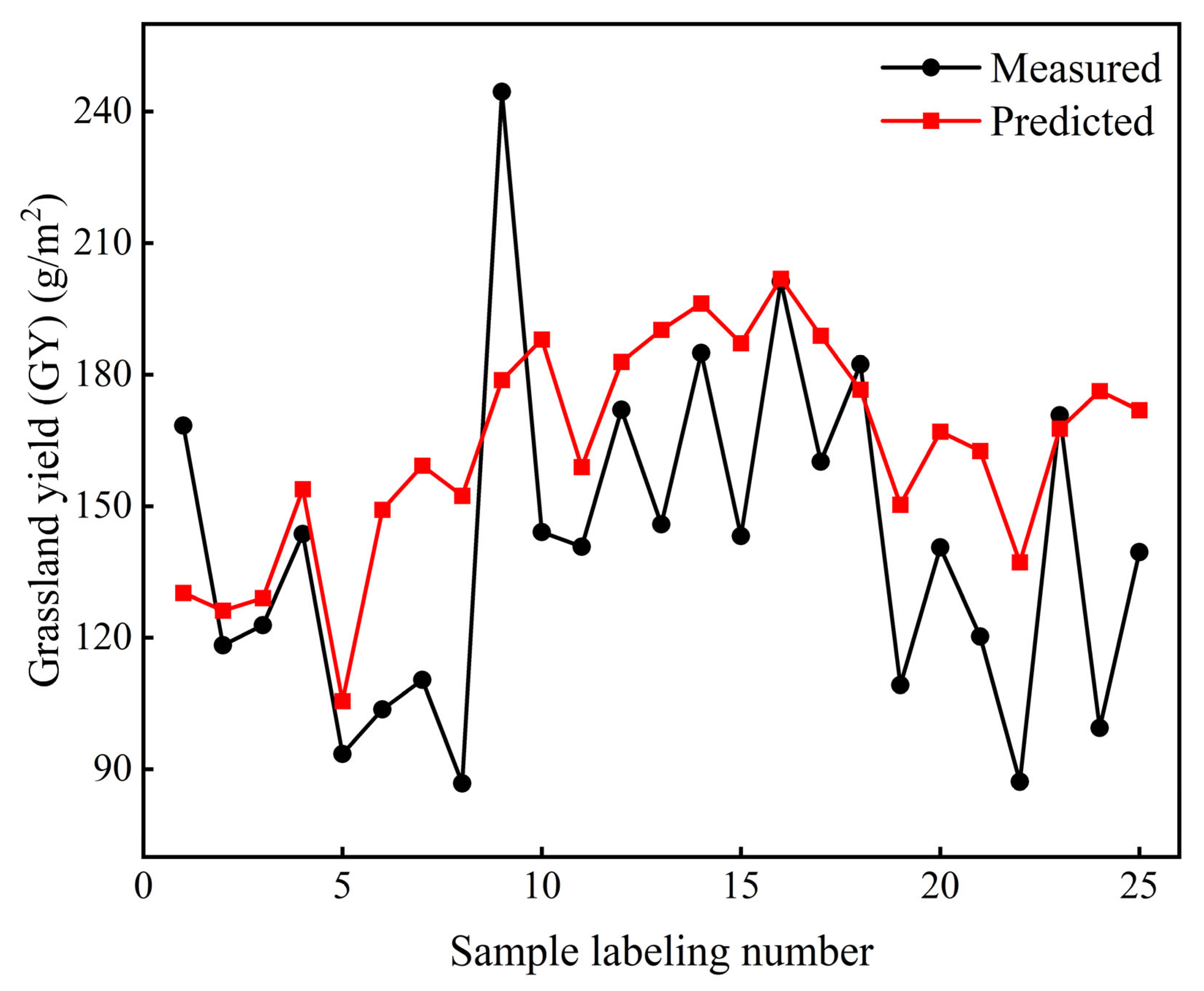
Based on the measurement of aboveground biomass from 25 grassland plots (0.5 m × 0.5 m) collected in the field in 2024, the grassland yield derived from the model was validated using the RMSE and EA. The validation results showed that the RMSE was 37.88 g/m2 and the EA was 73.52% (Figure 2). Previous studies on grassland yield estimation in Mongolia, which employed sparse sampling points along the China–Mongolia railway (Mongolian section), reported estimation accuracies ranging from 69% to 80% [40]. The estimation accuracy obtained in this study fell within the range of those earlier studies, which indicated that the results were suitable for subsequent applications.

3.2. Temporal Change Characteristics of Grassland Yield

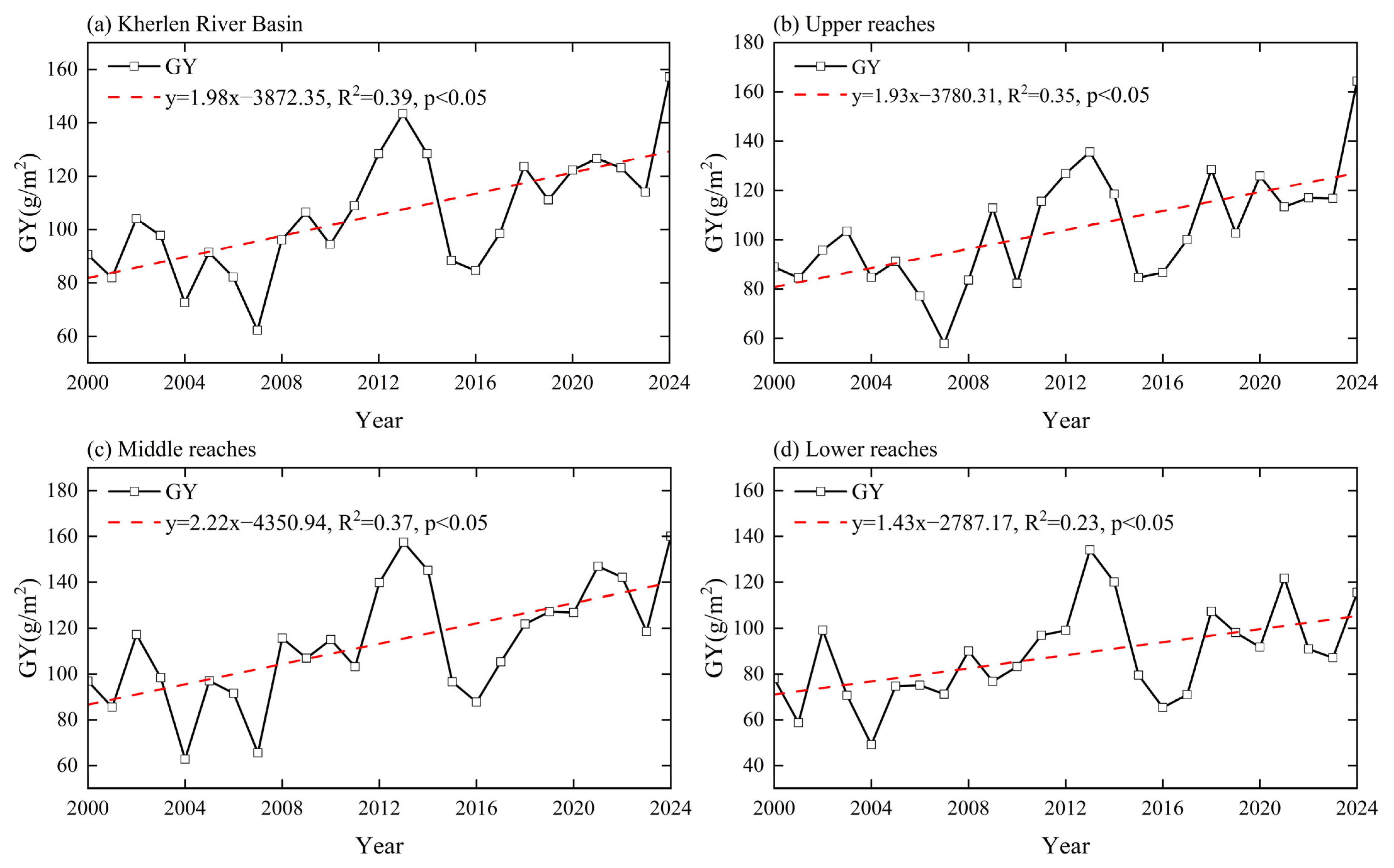
From 2000 to 2024, grassland yield in the Kherlen River Basin ranged from 62.26 g/m2 to 157.15 g/m2, with a mean of 105.53 g/m2. The highest yield occurred in 2024 (157.15 g/m2), exceeding the mean by 51.62 g/m2, while the lowest yield was observed in 2007 (62.26 g/m2), 43.27 g/m2 below the mean. Overall, the basin exhibited a significant linear increasing trend in grassland yield, with a growth rate of 1.98 g/(m2·a) (p < 0.05) (Figure 3a). Distinct spatial differences in grassland yield were observed among the upper, middle, and lower reaches of the basin. In the upper reaches, grassland yield ranged from 57.92 to 164.40 g/m2, with a mean of 103.99 g/m2. The maximum yield was recorded in 2024 (164.40 g/m2), 60.41 g/m2 above the mean, while the minimum occurred in 2007 (57.92 g/m2), 46.06 g/m2 below the mean. The upper reaches exhibited a significant linear increasing trend at a rate of 1.93 g/(m2·a) (p < 0.05), slightly lower than the basin-wide rate (Figure 3b). In the middle reaches, the yield varied between 62.80 and 160.14 g/m2, with a mean of 113.28 g/m2. The maximum yield occurred in 2024 (160.14 g/m2), 46.86 g/m2 higher than the mean, while the minimum was observed in 2004 (62.80 g/m2), 50.49 g/m2 lower than the mean. The middle reaches showed a significant linear increase at a rate of 2.22 g/(m2·a) (p < 0.05), which was higher than the basin-wide trend (Figure 3c). In contrast, the lower reaches showed yields ranging from 49.12 to 134.14 g/m2, with a mean of 88.23 g/m2. The highest yield was observed in 2013 (134.14 g/m2), 45.91 g/m2 above the mean, and its peak value occurred in a different year compared with other regions, which may be partly attributed to direct factors such as precipitation and grazing intensity, while the lowest yield occurred in 2004 (49.12 g/m2), 39.11 g/m2 below the mean. The lower reaches exhibited a significant linear increase at a rate of 1.43 g/(m2·a) (p < 0.05), which was substantially lower than the basin-wide rate (Figure 3d). Therefore, grassland yield in the Kherlen River Basin exhibited a significant linear increase from 2000 to 2024, with the rate of increase in the middle reaches exceeding that of the upper and lower reaches.

3.3. Spatial Changes in Grassland Yield

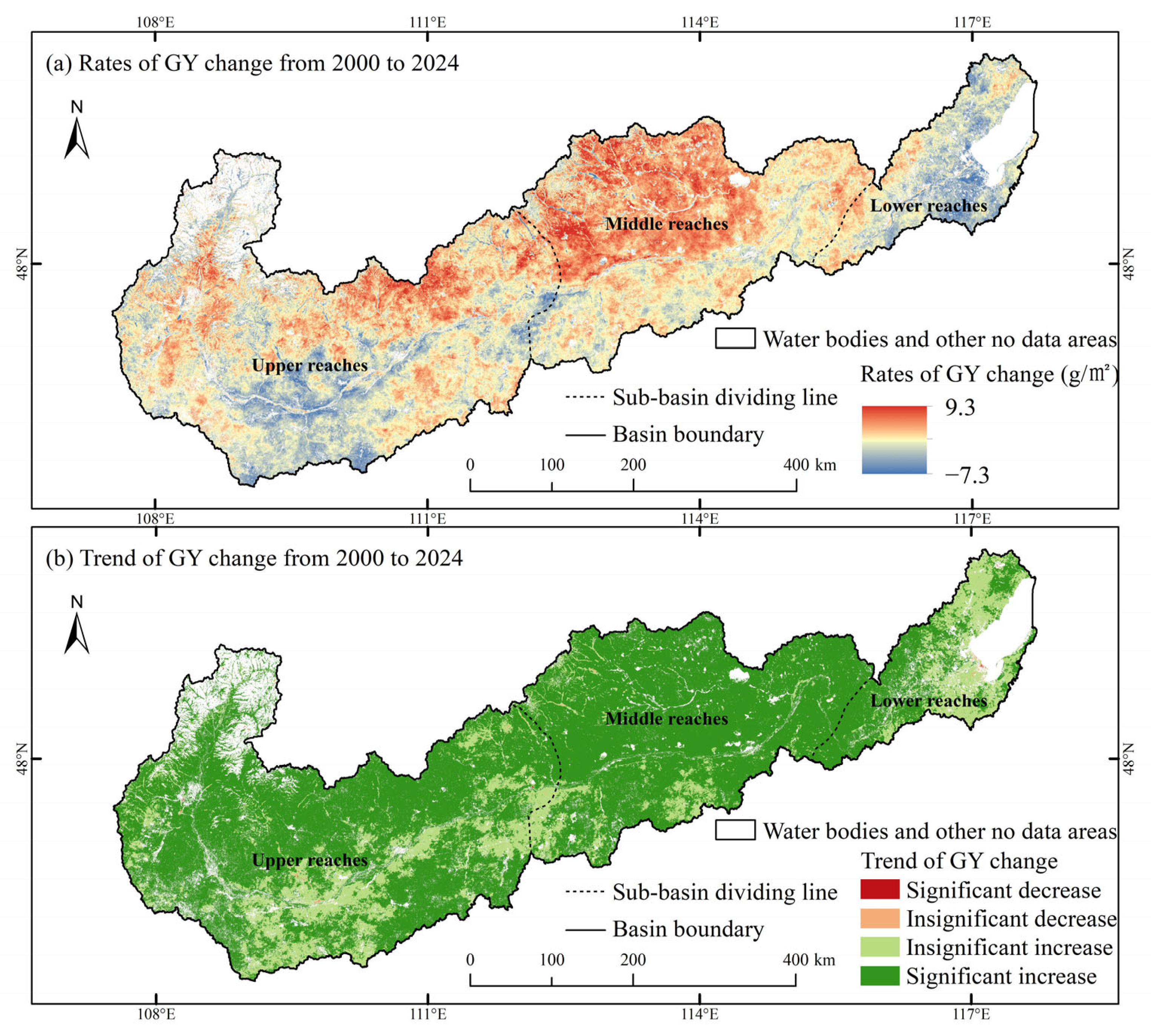
Between 2000 and 2024, grassland yield in the Kherlen River Basin primarily exhibited an increasing trend (Figure 4a), accounting for 99.82% of the basin’s area. Among these, areas with a significant increase accounted for 79.78% and were mainly distributed in the central and western parts of the basin, while areas with a significant decrease accounted for only 0.03% and were scattered along riverbanks. The spatial distribution of grassland yield changes varied across the upper, middle, and lower reaches of the basin. In the upper reaches, grassland yield was mainly characterized by an increasing trend, representing 51.85% of the total basin area. Areas with a significant increase accounted for 40.36% and were primarily concentrated in the northern sector of the upper reaches. Areas with a significant decrease constituted only 0.01% of the total basin area and were sporadically located within the mountainous regions of Töv Province and along rivers in Ulaanbaatar and Hentiy Province, Mongolia. In the middle reaches, grassland yield also showed a predominantly increasing trend, covering 36.39% of the total basin area. Regions with a significant increase accounted for 32.89% and were mainly located in the northern and eastern parts of the middle reaches. Areas with a significant decrease represented only 0.01% of the total basin area and were sporadically distributed along rivers in Sühbaatar Province and Dornod Province, Mongolia. Similarly, in the lower reaches, grassland yield was dominated by an increasing trend, accounting for 11.58% of the total basin area. Regions with a significant increase accounted for 6.53% and were primarily concentrated in the southwestern part of the lower reaches. Areas with a significant decrease represented only 0.01% of the total basin area and were mainly distributed along the southwestern shoreline of Hulun Lake (Figure 4b). Therefore, the grassland yield in the Kherlen River Basin exhibited a significant overall increasing trend during 2000–2024, with the proportion of areas showing a significant increase in grassland yield being higher in the upper reaches (40.36%) than in the middle (32.89%) and lower reaches (6.53%). The overall increase in grassland yield may be associated with a period of warmer and wetter climate conditions, while the spatial heterogeneity among regions could be attributed, on the one hand, to the regional effects of climate change and, on the other hand, to factors such as grazing activities, industrial production, and ecological policies.

3.4. Driving Factors of Grassland Yield

3.4.1. Single-Factor Impact Analysis of Grassland Yield

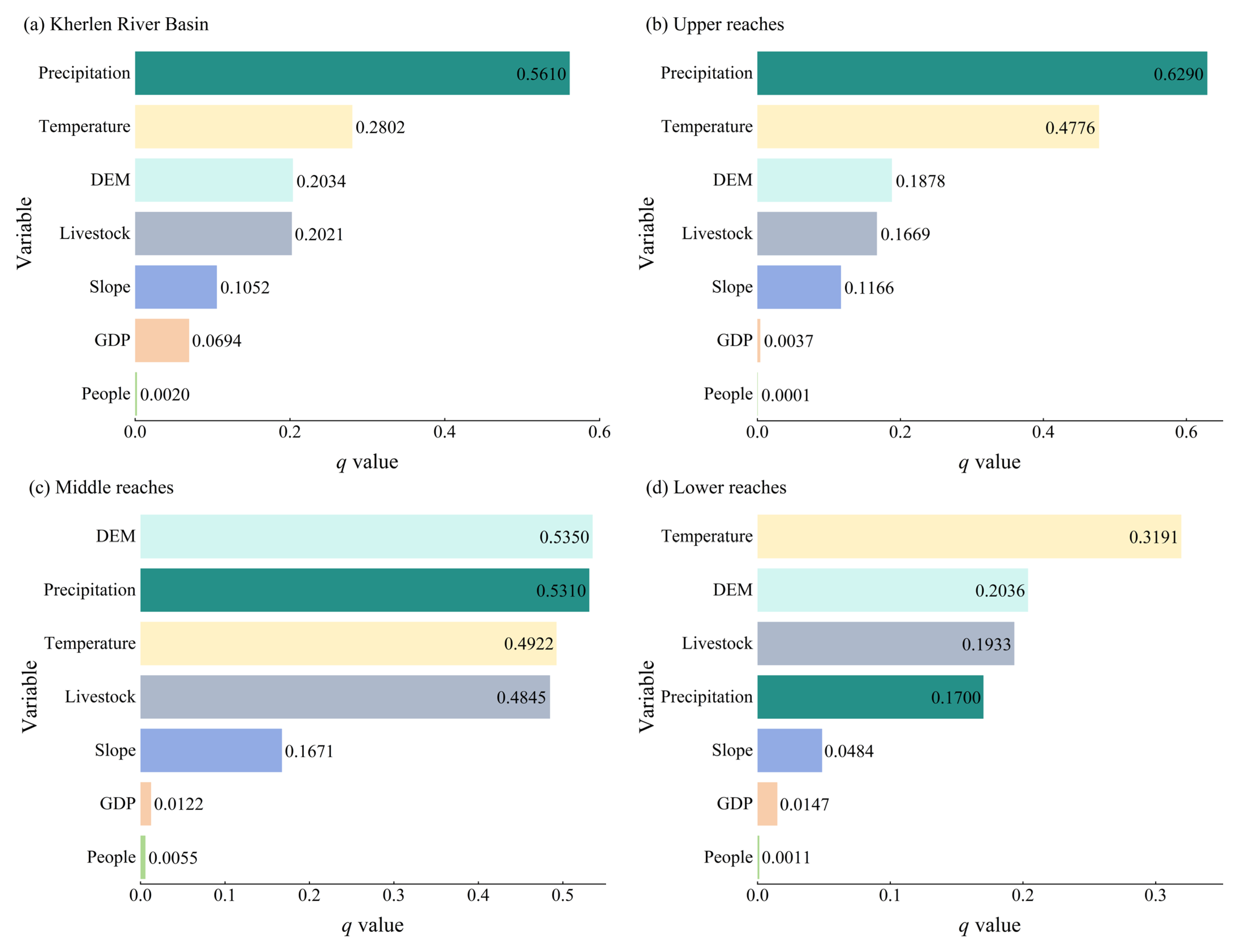
Based on the natural and anthropogenic characteristics of the Kherlen River Basin, this study selected seven factors—annual mean temperature, precipitation, livestock numbers, number of people, GDP, DEM-derived elevation, and slope—to investigate the driving forces of grassland yield variation. The ranking of the influence intensity (q values) of these factors on grassland yield change was as follows: precipitation (0.5610) > temperature (0.2802) > DEM (0.2034) > livestock (0.2021) > slope (0.1052) > GDP (0.0694) > people (0.0020). Among them, the population factor did not pass the significance test (Table 4). The results indicated that, at the single-factor level, climatic factors were the dominant drivers of grassland yield change in the Kherlen River Basin during 2000–2020, while the overall impact of human activities on grassland yield change was relatively minor (Figure 5a).
Single-factor driving analysis of different sub-basins revealed that, in the upper reaches of the Kherlen River Basin, precipitation and temperature exerted the strongest effects on grassland yield variation, with q values of 0.6290 and 0.4776, respectively, followed by DEM (q = 0.1878) and livestock (q = 0.1669). Anthropogenic factors had relatively minor impacts on grassland yield change in the upper reaches. Among them, people did not pass the significance tests corrected by the Bonferroni, Holm, and Benjamini–Hochberg (BH-FDR) methods, while GDP did not pass the Bonferroni and Holm corrections. Therefore, at the single-factor level, climatic factors were the dominant drivers of grassland yield change in the upper reaches (Figure 5b). In the middle reaches, DEM had the strongest effect (q = 0.5350), followed by precipitation (q = 0.5310), temperature (q = 0.4922), and livestock (q = 0.4845). In contrast, slope, GDP, and people exerted weaker influences, with both people and GDP failing to pass the significance tests corrected by the Bonferroni, Holm, and Benjamini–Hochberg methods. Consequently, DEM, climatic factors, and livestock were recognized as the primary factors influencing changes in grassland yield in the middle reaches (Figure 5c). In the lower reaches, temperature was the most influential factor (q = 0.3191), followed by DEM (q = 0.2036). Livestock (q = 0.1933) and precipitation (q = 0.1700) exhibited comparable impacts, while slope, GDP, and people had relatively minor effects. Notably, both people and GDP also failed to pass the significance tests corrected by the Bonferroni, Holm, and Benjamini–Hochberg methods. Therefore, at the single-factor level, the key drivers of grassland yield change in the lower reaches were climatic factors, DEM, and livestock (Figure 5d). In summary, climatic factors (precipitation and temperature) and the geographic variable (elevation) constitute the primary drivers of grassland yield variation in the Kherlen River Basin. Livestock numbers also passed the significance tests, indicating that grassland productivity in these areas is, to some extent, influenced by human activities.

3.4.2. Interaction Analysis of Factors Influencing Grassland Yield

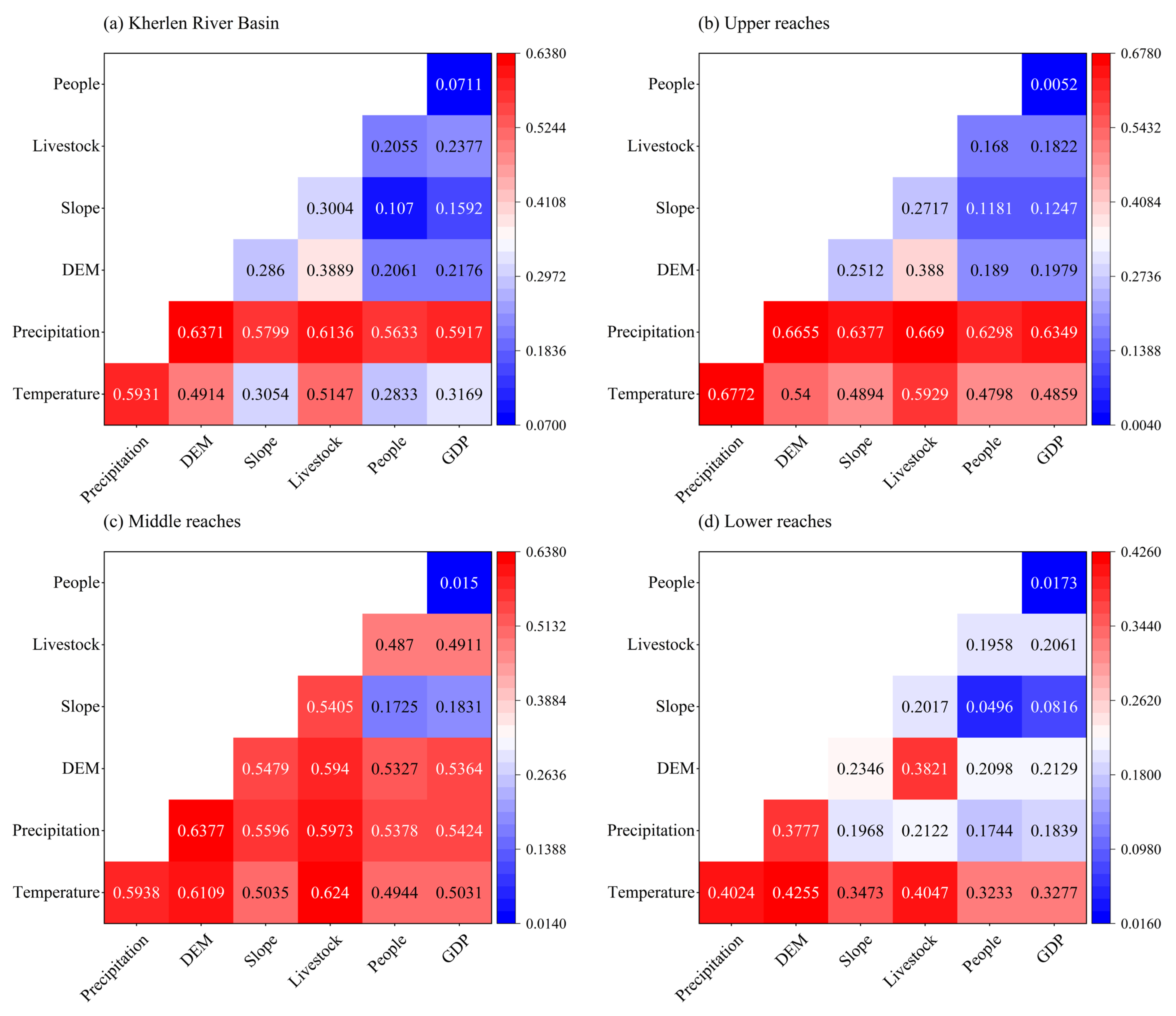
The results of interaction detector revealed that the interactions among factors influencing grassland yield variation in the Kherlen River Basin exhibited both bivariate and nonlinear enhancement effects, with the majority of interactions characterized as bivariate enhancement. Among them, the interaction between precipitation and DEM exerted the strongest effect on grassland yield variation (q = 0.6371), followed by the interaction between precipitation and livestock (q = 0.6136). In addition, the interactions of temperature with precipitation, precipitation with slope, precipitation with GDP, and precipitation with people also showed greater explanatory power than single-factor effects (Figure 6a). Therefore, the variation in grassland yield in the Kherlen River Basin was mainly driven by factor interactions, highlighting the necessity of analyzing interactions among factors in the upper, middle, and lower reaches of the basin.
In the upper reaches of the Kherlen River Basin, most factor interactions also exhibited bivariate enhancement. Among these, the interaction between temperature and precipitation had the greatest effect on grassland yield variation (q = 0.6772). The interactions of precipitation with livestock, DEM, slope, GDP, and people also showed stronger explanatory power than single factors, with q values of 0.6690, 0.6655, 0.6377, 0.6349, and 0.6298, respectively (Figure 6b). In the middle reaches of the basin, most factor interactions were likewise characterized by bivariate enhancement. The interaction between precipitation and DEM exerted the strongest influence on grassland yield variation (q = 0.6377), followed by the interactions of temperature with livestock and DEM, with q values of 0.6240 and 0.6109, respectively. In addition, the interactions of temperature with precipitation, precipitation with slope, livestock, people, GDP, DEM with slope, livestock, GDP, slope with livestock also showed greater effects than single factors (Figure 6c). In the lower reaches, most factor interactions similarly displayed bivariate enhancement, with the interaction between temperature and DEM having the strongest effect (q = 0.4255). This was followed by the interactions of temperature with livestock (q = 0.4047) and precipitation (q = 0.4024). Moreover, the interactions of DEM with livestock, precipitation with DEM, and temperature with slope, people, and GDP also showed stronger explanatory power than single factors (Figure 6d).

3.4.3. Ecological Detector Analysis of Factors Influencing Grassland Yield

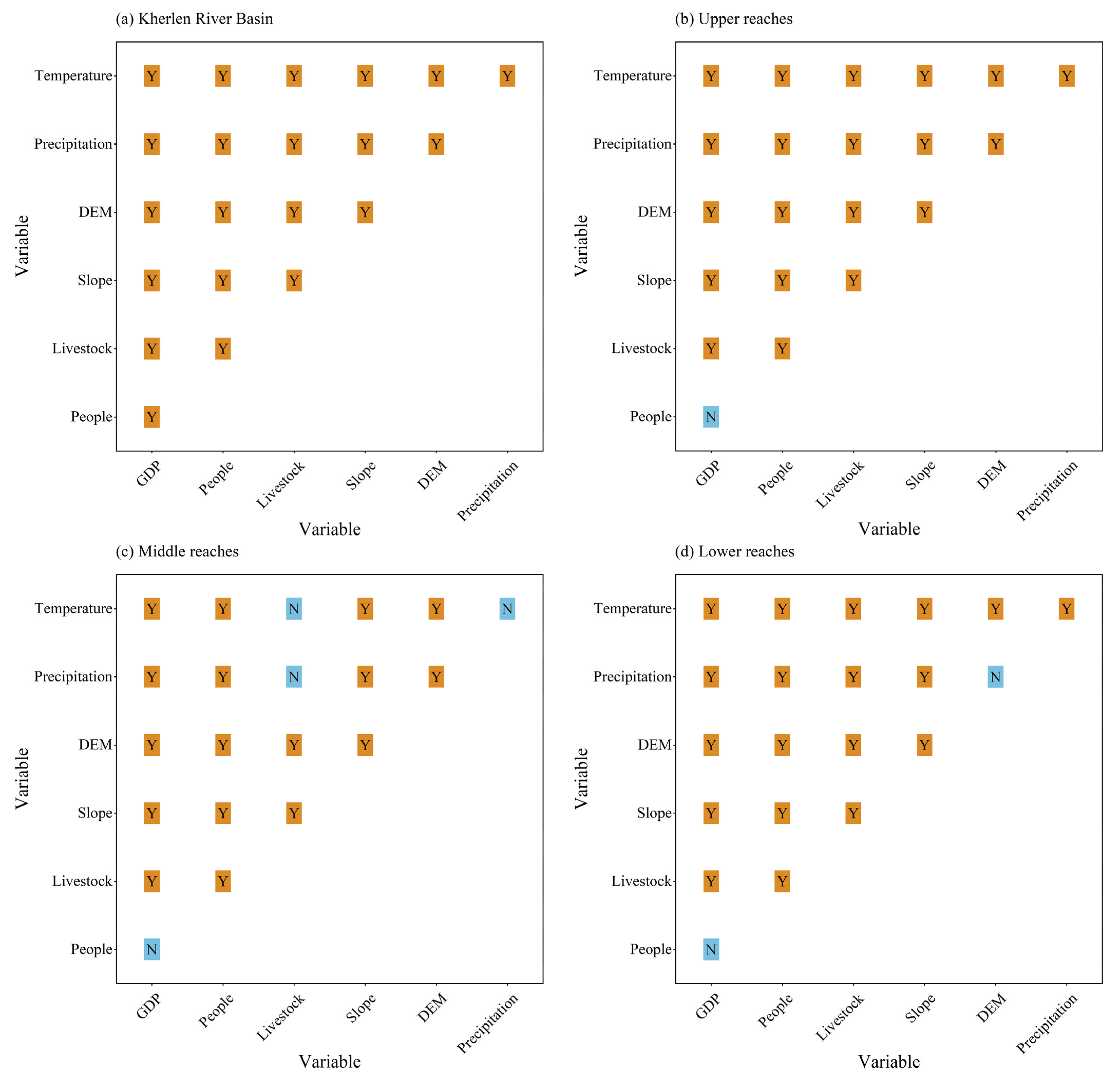
The ecological detector was employed to analyze the statistical significance of the combined effects of two influencing factors on the spatial distribution of grassland yield. The ecological detector results for all factor pairs in the Kherlen River Basin were significant, indicating reliability at the 95% confidence level. This suggested that the effects of different factor pairs on the spatial distribution of grassland yield differed significantly (Figure 7a).
At the 95% confidence level, in the upper reaches of the Kherlen River Basin, temperature, precipitation, DEM, slope, livestock, and other factors exhibited significant differences in their effects on the spatial distribution of grassland yield, whereas people and GDP showed no significant difference (Figure 7b). In the middle reaches, no significant differences were observed between temperature and precipitation, temperature and livestock, precipitation and livestock, or people and GDP in their effects on grassland yield distribution (Figure 7c). In the lower reaches, temperature, slope, livestock, and other factors showed significant differences in their effects, while precipitation and DEM, as well as people and GDP, did not exhibit significant differences (Figure 7d). Overall, in the Kherlen River Basin, the effects of interactions among natural factors on the spatiotemporal distribution of grassland yield were stronger than those between natural and anthropogenic factors.

4. Discussion

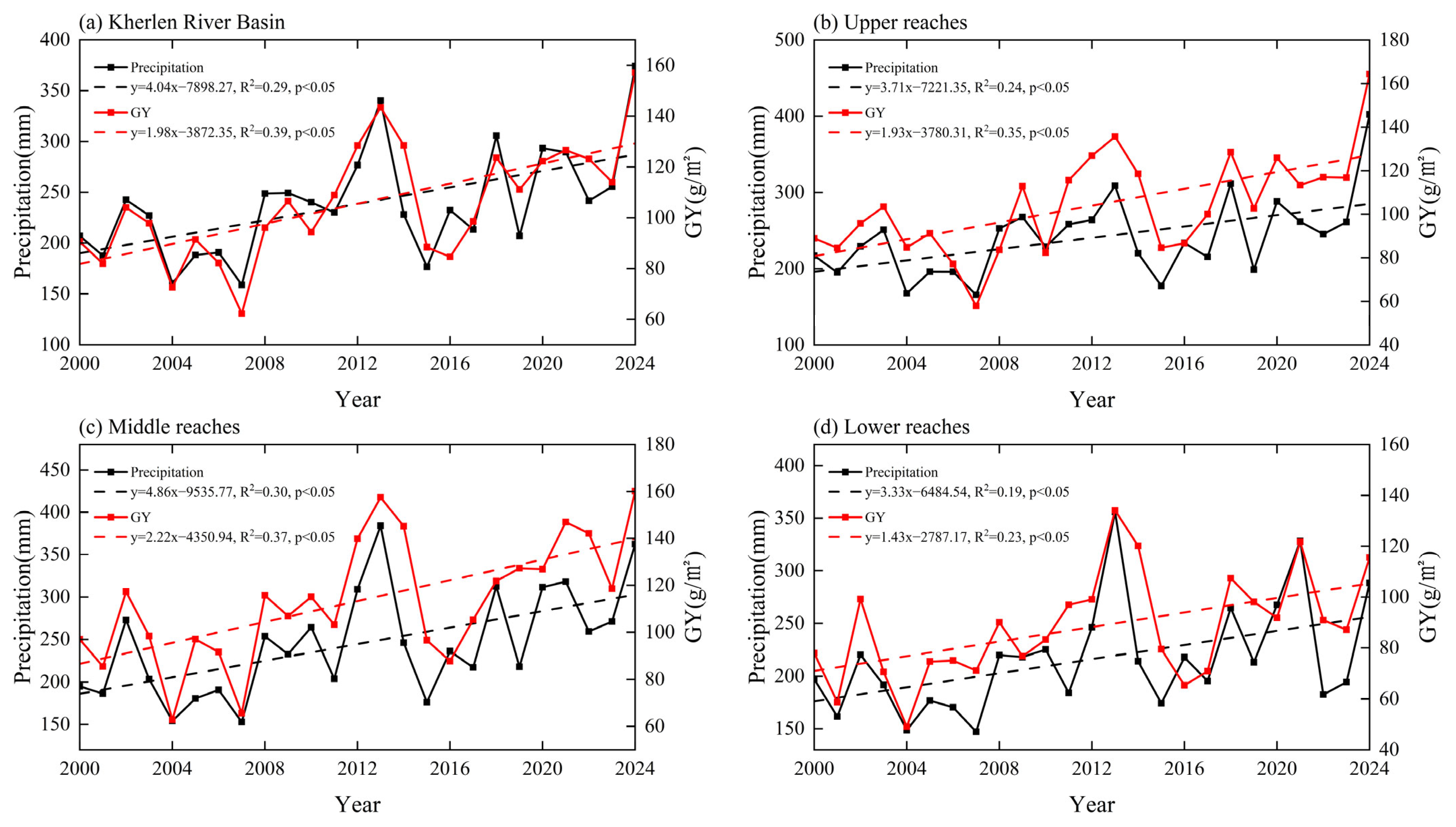
As part of the China–Russia–Mongolia Economic Corridor, the Kherlen River Basin provides high biodiversity value to Mongolia and neighboring countries and plays an important role in maintaining local ecosystem balance. Comprehensive and coordinated management of the transboundary river basin is essential for preserving the natural resilience of local ecosystems and adapting to rapidly changing climatic conditions. This study revealed the spatiotemporal variation characteristics of grassland yield in the Kherlen River Basin during 2000–2024. In terms of temporal variation, the multi-year mean grassland yield in the basin remained at approximately 106.23 g/m2, showing a significant linear increasing trend. This outcome aligns well with earlier evidence regarding the temporal variation in grassland yield across the Mongolian Plateau from 2000 to 2020 [9]. The interannual variations in grassland yield and climatic factors (temperature and precipitation) in the Kherlen River Basin were compared and analyzed (Figure 8), revealing that grassland yield exhibited a strong correspondence with precipitation dynamics. Precipitation in the basin reached its lowest levels in 2004 and 2007, which likely contributed to the minimum grassland yield observed in 2007 for the basin as a whole and for the upper reaches, and in 2004 for the middle and lower reaches. Unlike the other subregions, the lower reaches experienced the highest grassland yield in 2013. This anomaly was likely driven by exceptionally high precipitation in that year, which reached 356 mm—the maximum recorded during 2000–2024—and was markedly higher than the 288.38 mm observed in 2024. This also indicates that precipitation is the primary factor influencing grassland ecosystems in arid and semiarid regions [41,42]. Regarding spatial variation, grassland yield in the Kherlen River Basin generally increased during 2000–2024, with the area of significant increase in the upper reaches exceeding that in the middle and lower reaches, which is consistent with the findings of other scholars [43].
The grassland yield in the Kherlen River Basin was generally more sensitive to variations in natural factors than to anthropogenic factors, as indicated by higher q-values for the former. Among these, temperature and precipitation were identified as the primary drivers of grassland yield variation, which is largely consistent with recent studies [17,43]. Regarding the effects of individual factors, precipitation exerted the strongest influence on grassland yield variation across the entire basin. Specifically, the dominant single factors affecting grassland yield variation in the upper, middle, and lower reaches were precipitation, DEM, and temperature, respectively. Moreover, the analyses of the upper, middle, and lower reaches indicate that the spatial association between livestock numbers and grassland yield is stronger in the middle and lower reaches than in the upper reaches. This may be attributed to the higher elevation, more rugged terrain, and lower grazing intensity in the upper reaches. However, due to factors such as the resolution of the socioeconomic data, the influence of livestock numbers on grassland yield was not effectively reflected in the subsequent interaction analyses across the different river segments. In terms of factor interactions, the interaction between precipitation and DEM had the greatest impact on grassland yield variation in the Kherlen River Basin. At the sub-basin scale, the interactions between temperature and precipitation, precipitation and elevation, and temperature and elevation were the most influential in the upper, middle, and lower reaches, respectively. Among these, elevation regulates the effectiveness of temperature and precipitation by influencing the vertical differentiation of hydrothermal conditions, thereby playing a critical role in shaping the spatial distribution pattern of grassland yield through its interaction with climatic factors [44]. This finding indicates that the grassland yield in the Kherlen River Basin is more sensitive to the vertical climatic gradient than to the horizontal gradient.
Therefore, in the upper reaches, where grassland yield is highly sensitive to climatic fluctuations, management efforts should focus on climate adaptation and ecological restoration. In the middle reaches, where grassland yield exhibits the fastest growth, emphasis should be placed on optimizing land-use structure and enhancing soil and water conservation. In the lower reaches, where productivity is strongly dependent on precipitation, priority should be given to water resource regulation and drought adaptation management.
This study comprehensively analyzed the driving mechanisms of grassland yield variation in the Kherlen River Basin by integrating both natural and anthropogenic factors. However, the relatively coarse spatial resolution of socioeconomic data may have limited the accuracy of assessing human-induced impacts, thereby introducing a certain degree of uncertainty into the analysis. Moreover, although the Geodetector model offers several advantages—such as computational simplicity, no requirement for distributional assumptions, and the ability to identify factor interactions—it primarily focuses on spatial differentiation and has limited capacity to characterize temporal dynamics. Therefore, future studies could incorporate higher-resolution datasets and integrate time-series analysis with spatial differentiation approaches to achieve more detailed and comprehensive assessments.

5. Conclusions

(1) The RMSE between the model-estimated grassland yield of the Kherlen River Basin in 2024 and the measured aboveground biomass from field quadrats in the same year was 37.88 g/m2, with an EA of 73.52%, indicating that the model was suitable for analyzing the spatiotemporal variation in grassland yield within the basin.
(2) From 2000 to 2024, the grassland yield in the Kherlen River Basin exhibited a significant linear increasing trend, with an overall growth rate of 1.98 g/(m2·a) (p < 0.05). Specifically, the growth rates in the upper, middle, and lower reaches were 1.93 g/(m2·a) (p < 0.05), 2.22 g/(m2·a) (p < 0.05), and 1.43 g/(m2·a) (p < 0.05), respectively.
(3) From 2000 to 2024, grassland yield in the Kherlen River Basin was dominated by an increasing trend, with areas exhibiting a significant increase accounting for 79.78% of the total basin area, primarily distributed in the central and western regions. In contrast, areas showing a significant decrease accounted for only 0.03% of the basin area, sporadically distributed along the riverbanks. A comparison across the upper, middle, and lower reaches revealed that all sub-basins were predominantly characterized by significant increasing trends. Specifically, regions with significantly increasing grassland yield in the upper, middle, and lower reaches accounted for 40.36%, 32.89%, and 6.53% of the total basin area, respectively, mainly concentrated in the northern part of the upper reaches, the northern and eastern parts of the middle reaches, and the southwestern part of the lower reaches.
(4) From 2000 to 2020, single-factor analysis showed that precipitation was the dominant factor influencing grassland yield change in the Kherlen River Basin, while the primary factors in the upper, middle, and lower reaches were precipitation, DEM, and temperature, respectively. In the interaction analysis, the interaction between precipitation and DEM emerged as the strongest driver of grassland yield change at the basin scale, whereas the most influential interaction factors were temperature and precipitation in the upper reaches, precipitation and DEM in the middle reaches, and temperature and DEM in the lower reaches. The ecological detector results indicated that significant spatial differences existed in the effects of most factors on the spatial distribution of grassland yield change across the overall basin as well as within the upper, middle, and lower reaches.

Author Contributions

Conceptualization, M.Y., H.Y. and T.W.; methodology, M.Y. and T.W.; software, H.Y.; vali-dation, M.Y., T.W. and Y.S.; formal analysis, M.Y., H.Y. and T.W.; investigation, M.Y., T.W., J.W. and T.L.; resources, P.L., J.Z. and B.W.; data curation, M.Y., H.Y. and T.W.; writing—original draft preparation, M.Y., H.Y. and T.W.; writing—review and editing, M.Y. and T.W.; visualization, M.Y., H.Y. and T.W.; supervision, P.L.; project administration, P.L.; funding acquisition, P.L., J.Z. and B.W. All authors have read and agreed to the published version of the manuscript.

Funding

This research was funded by the National Key R&D Program of China (No. 2022YFE0119200), Natural Science Basic Research Program of Shaanxi (No. 2024JC-YBQN-0306), and Survey, Monitoring, and Assessment of the Interaction of Natural Resource Elements and Ecological Degradation in the Transition Zone between the Qinling Mountains and the Loess Plateau (No. DD20220882).

Data Availability Statement

The datasets employed in this study are included in the article, and any additional inquiries may be addressed to the corresponding author.

Conflicts of Interest

The authors declare no conflicts of interest.

References

  1. Chen, M.; Shao, Q.; Ning, J.; Liu, G.; Liu, S.; Niu, L.; Zhang, X.; Huang, H. Analysis on ecological restoration in different ecogeographical divisions of the Tibetan Plateau. Acta Agrestia Sin. 2023, 31, 1211–1225. [Google Scholar] [CrossRef]
  2. Wu, N.; Liu, G.; Liu, A.; Bai, H.; Chao, L. Monitoring and driving force analysis of net primary productivity in native grassland: A case study in Xilingol steppe, China. J. Appl. Ecol. 2020, 31, 1233–1240. [Google Scholar] [CrossRef]
  3. Eisavi, V.; Homayouni, S.; Yazdi, A.; Alimohammadi, A. Land cover mapping based on random forest classification of multitemporal spectral and thermal images. Environ. Monit. Assess. 2015, 187, 291. [Google Scholar] [CrossRef] [PubMed]
  4. Yang, J.; Wan, Z.; Borjigin, S.; Zhang, D.; Yan, Y.; Chen, Y.; Gu, R.; Gao, Q. Changing trends of NDVI and their responses to climatic variation in different types of grassland in Inner Mongolia from 1982 to 2011. Sustainability 2019, 11, 3256. [Google Scholar] [CrossRef]
  5. Chen, C.; Jing, C.; Zhao, W.; Xu, Y. Grassland quality response to climate change in Xinjiang and predicted future trends. Acta Pratac. Sin. 2022, 31, 1–16. [Google Scholar] [CrossRef]
  6. Wang, Q.; Okadera, T.; Nakayama, T.; Batkhishig, O.; Bayarsaikhan, U. Estimation of the carrying capacity and relative stocking density of Mongolian grasslands under various adaptation scenarios. Sci. Total Environ. 2024, 913, 169772. [Google Scholar] [CrossRef]
  7. Tuo, D.; Lu, Q.; Que, X.; Cheng, L.; Yang, Y.; Gao, P.; Cui, G. Evaluation of grassland ecosystem services in northern China. Acta Ecol. Sin. 2024, 44, 455–462. [Google Scholar] [CrossRef]
  8. Umuhoza, J.; Jiapaer, G.; Yin, H.; Mind’je, R.; Gasirabo, A.; Nzabarinda, V.; Umwali, E. The analysis of grassland carrying capacity and its impact factors in typical mountain areas in Central Asia—A case of Kyrgyzstan and Tajikistan. Ecol. Indic. 2021, 131, 108129. [Google Scholar] [CrossRef]
  9. Li, M.; Wang, J.; Li, K.; Ochir, A.; Togtokh, C.; Xu, C. Spatial-temporal pattern analysis of grassland yield in Mongolian Plateau based on artificial neural network. Remote Sens. 2023, 15, 3968. [Google Scholar] [CrossRef]
  10. Xu, B.; Yang, X.; Jin, Y.; Wang, D.; Yang, Z.; Li, J.; Liu, H.; Yu, H.; Ma, H. Monitoring and evaluation of grassland-livestock balance in pastoral and semi-pastoral counties of China. Geogr. Res. 2012, 31, 1998–2006. [Google Scholar] [CrossRef]
  11. Reinermann, S.; Asam, S.; Kuenzer, C. Remote sensing of grassland production and management—A review. Remote Sens. 2020, 12, 1949. [Google Scholar] [CrossRef]
  12. Ullah, S.; Si, Y.; Schlerf, M.; Skidmore, A.; Shafique, M.; Iqbal, I. Estimation of grassland biomass and nitrogen using MERIS data. Int. J. Appl. Earth Obs. 2012, 19, 196–204. [Google Scholar] [CrossRef]
  13. Eisfelder, C.; Klein, I.; Bekkuliyeva, A.; Kuenzer, C.; Buchroithner, M.; Dech, S. Above-ground biomass estimation based on NPP time-series—A novel approach for biomass estimation in semi-arid Kazakhstan. Ecol. Indic. 2017, 72, 13–22. [Google Scholar] [CrossRef]
  14. Punalekar, S.; Verhoef, A.; Quaife, T.; Humphries, D.; Bermingham, L.; Reynolds, C. Application of Sentinel-2A data for pasture biomass monitoring using a physically based radiative transfer model. Remote Sens. Environ. 2018, 218, 207–220. [Google Scholar] [CrossRef]
  15. He, L.; Li, A.; Yin, G.; Nan, X.; Bian, J. Retrieval of grassland aboveground biomass through inversion of the PROSAIL model with MODIS imagery. Remote Sens. 2019, 11, 1597. [Google Scholar] [CrossRef]
  16. Ye, S.; Han, X.; Liu, Y.; He, T.; Wu, Y. Estimation of net primary productivity in Inner Mongolia grassland based on optimized CASA model parameters. Inner Mong. For. Investig. Des. 2025, 48, 62–67. [Google Scholar] [CrossRef]
  17. Yin, C.; Chen, X.; Luo, M.; Meng, F.; Sa, C.; Bao, S.; Yuan, Z.; Zhang, X.; Bao, Y. Quantifying the contribution of driving factors on distribution and change of net primary productivity of vegetation in the Mongolian Plateau. Remote Sens. 2023, 15, 1986. [Google Scholar] [CrossRef]
  18. Bao, G.; Tuya, A.; Bayarsaikhan, S.; Dorjsuren, A.; Mandakh, U.; Bao, Y.; Li, C.; Vanchindorj, B. Variations and climate constraints of terrestrial net primary productivity over Mongolia. Quat. Int. 2020, 537, 112–125. [Google Scholar] [CrossRef]
  19. Sun, B.; Qin, P.; Yue, W.; Guo, Y.; Gao, Z.; Wang, Y.; Li, Y.; Yan, Z. High temporal and spatial estimation of grass yield by applying an improved Carnegie-Ames-Stanford approach (CASA)-NPP transformation method: A case study of Zhenglan Banner, Inner Mongolia, China. Comput. Electron. Agric. 2024, 224, 109134. [Google Scholar] [CrossRef]
  20. Yan, N.; Zhu, W.; Wu, B.; Tuvdendorj, B.; Chang, S.; Mishigdorj, O.; Zhang, X. Assessment of the grassland carrying capacity for winter-spring period in Mongolia. Ecol. Indic. 2023, 146, 109868. [Google Scholar] [CrossRef]
  21. Chen, H.; Ma, C.; Yan, L. Analysis of climate change and its impact on grass yield of natural grassland in Henan County Qinghai Province from 1981 to 2022. Qinghai Pratac. 2023, 32, 71–75. [Google Scholar] [CrossRef]
  22. Xu, Y.; Dai, Q.; Lu, Y.; Zhao, C.; Huang, W.; Xu, M.; Feng, Y. Identification of ecologically sensitive zones affected by climate change and anthropogenic activities in Southwest China through a NDVI-based spatial-temporal model. Ecol. Indic. 2024, 158, 111482. [Google Scholar] [CrossRef]
  23. Wang, J.; Xu, C. Geodetector: Principle and prospective. Acta Geogr. Sin. 2017, 72, 116–134. [Google Scholar] [CrossRef]
  24. Yu, S.; Du, W.; Zhang, X.; Hong, Y.; Liu, Y.; Hong, M.; Chen, S. Spatiotemporal changes in NDVI and its driving factors in the Kherlen River Basin. Chin. Geogr. Sci. 2023, 33, 377–392. [Google Scholar] [CrossRef]
  25. Wang, Z.; Che, T.; Dai, L.; Jiang, Y. Comparative analysis on the spatiotemporal changes of vegetation and drivers in inland river basins of the Hexi Corridor, China. IEEE J. Sel. Top. Appl. Earth Obs. Remote Sens. 2025, 18, 8112–8124. [Google Scholar] [CrossRef]
  26. Wu, Y.; Zhang, F.; Pei, H.; Jiang, J. The effect of temperature and precipitation during the growing season on the biomass of steppe communities in the Herlen Basin, northern China. Acta Pratac. Sin. 2012, 21, 227–232. [Google Scholar] [CrossRef]
  27. Cheng, J.; Mao, D.; Yu, S.; Wang, Z.; Xiang, H. Temporal and spatial changes of grassland in Kherlen River Basin from 1980 to 2020. Bull. Soil Water Conserv. 2022, 42, 296–303. [Google Scholar] [CrossRef]
  28. Kummu, M.; Kosonen, M.; Sayyar, S. Downscaled gridded global dataset for gross domestic product (GDP) per capita PPP over 1990–2022. Sci. Data 2025, 12, 178. [Google Scholar] [CrossRef]
  29. Wang, Y.; Lyu, J.; Li, Z.; Mu, W.; Wan, F. Spatiotemporal dynamics of vegetation NPP and its driving factors in Yiluo River Basin. J. North China Univ. Water Resour. Electr. Power (Nat. Sci. Ed.) 2025, 46, 37–49. [Google Scholar] [CrossRef]
  30. Zhu, W.; Pan, Y.; Long, Z.; Chen, Y.; Li, J.; Hu, H. Estimating net primary productivity of terrestrial vegetation based on GIS and RS: A case study in Inner Mongolia, China. Natl. Remote Sens. Bull. 2005, 9, 300–307. [Google Scholar] [CrossRef]
  31. Zhu, W.; Pan, Y.; Zhang, J. Estimation of net primary productivity of Chinese terrestrial vegetation based on remote sensing. Chin. J. Plant. Ecol. 2007, 31, 413–424. [Google Scholar] [CrossRef]
  32. Zhang, X. The potential evapotranspiration (PE) index for vegetation and vegetation-climatic classification (1)—An introduction of main methods and PEP program. Chin. J. Plant Ecol. 1989, 13, 197. [Google Scholar] [CrossRef]
  33. Tang, X.; Zhang, F.; Feng, Q.; Ma, X. Changes in grassland yield and grassland-livestock balance in Ordos City over the past 20 years. Acta Ecol. Sin. 2024, 44, 10887–10896. [Google Scholar] [CrossRef]
  34. Yan, L.; Kong, L.; Zhang, L.; Ouyang, Z.; Hu, J. The definition, methods and key issues of grassland ecosystem carrying capacity. Chin. J. Eco Agric. 2022, 30, 1228–1237. [Google Scholar] [CrossRef]
  35. Peng, H.; Wang, S.; Wang, X. Consistency and asymptotic distribution of the Theil–Sen estimator. J. Stat. Plan. Inference 2008, 138, 1836–1850. [Google Scholar] [CrossRef]
  36. Xia, T.; Xue, X.; Wang, H.; Xu, W.; Sheng, Z.; Wang, Y. Changes in terrestrial water storage and its drivers on the north slope of Kunlun Mountains. Arid Land Geogr. 2024, 47, 1292–1303. [Google Scholar] [CrossRef]
  37. Zhang, H.; Li, J.; Tian, P.; Wang, Z.; Shen, X. Spatio-temporal evolution of habitat quality in the East China Sea continental coastal zone based on land use changes. Acta. Ecol. Sin. 2023, 43, 937–947. [Google Scholar] [CrossRef]
  38. Guo, Z.; Wei, W.; Shi, P.; Zhou, L.; Wang, X.; Li, Z.; Pang, S.; Xie, B. Spatiotemporal changes of land desertification sensitivity in the arid region of Northwest China. Acta Geogr. Sin. 2020, 75, 1949–1965. [Google Scholar] [CrossRef]
  39. Sun, Y.; Guan, Q.; Wang, Q.; Yang, L.; Pan, N.; Ma, Y.; Luo, H. Quantitative assessment of the impact of climatic factors on phenological changes in the Qilian Mountains, China. For. Ecol. Manag. 2021, 499, 119594. [Google Scholar] [CrossRef]
  40. Wang, Y.; Wang, J.; Wei, H.; Ochir, A.; Davaasuren, D.; Chonokhuu, S. Study on estimation method of Mongolia grassland production based on sparse samples. J. Geo Inf. Sci. 2020, 22, 1814–1822. [Google Scholar] [CrossRef]
  41. Li, C.; Li, L.; Wu, X.; Tsunekawa, A.; Wei, Y.; Liu, Y.; Peng, L.; Chen, J.; Bai, K. Increasing precipitation promoted vegetation growth in the Mongolian Plateau during 2001–2018. Front. Environ. Sci. 2023, 11, 1153601. [Google Scholar] [CrossRef]
  42. He, B.; Tuya, W.; Qinchaoketu, S.; Nanzad, L.; Yong, M.; Kesi, T.; Sun, C. Climate change characteristics of typical grassland in the Mongolian Plateau from 1978 to 2020. Sustainability 2022, 14, 16529. [Google Scholar] [CrossRef]
  43. Li, T.; Li, S.; Li, P.; Huang, J.; Wang, J.; Ochir, A.; Yang, M.; Wang, T.; Chan, F. Spatiotemporal variability in drivers of grassland degradation and recovery under economic transformation in Mongolia. J. Environ. Manag. 2025, 393, 127097. [Google Scholar] [CrossRef] [PubMed]
  44. Wang, Z.; Wang, Y.; Liu, Y.; Wang, F.; Deng, W.; Rao, P. Spatiotemporal characteristics and natural forces of grassland NDVI changes in Qilian Mountains from a sub-basin perspective. Ecol. Indic. 2023, 157, 111186. [Google Scholar] [CrossRef]
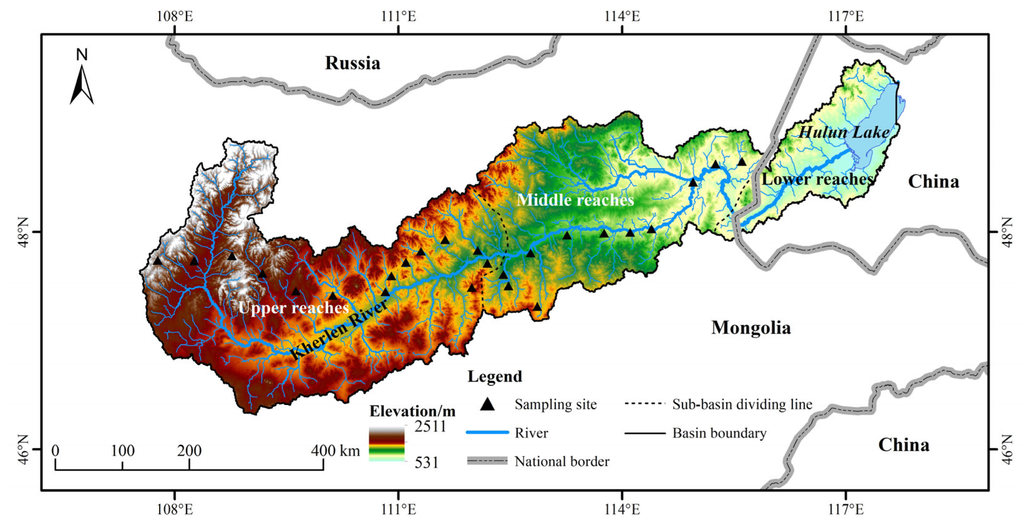
Figure 1. Sub-basin delineation and distribution of sampling sites in the study area.
Water 17 03397 g001
Figure 2. Validation of model-estimated grassland yield against field-measured values in the Kherlen River Basin.
Water 17 03397 g002
Figure 3. Interannual changes in grassland yield (GY) in the Kherlen River Basin from 2000 to 2024. (a) Kherlen River Basin; (b) Upper reaches; (c) Middle reaches; (d) Lower reaches.
Water 17 03397 g003
Figure 4. Spatial distribution of grassland yield (GY) change rates and change trends in the overall Kherlen River Basin and its upper, middle, and lower reaches from 2000 to 2024. (a) Rates of GY change from 2000 to 2024; (b) Trend of GY change from 2000 to 2024.
Water 17 03397 g004
Figure 5. Results of single-factor detector analysis of grassland yield in the overall Kherlen River Basin and its upper, middle, and lower reaches. (a) Kherlen River Basin; (b) Upper reaches; (c) Middle reaches; (d) Lower reaches.
Water 17 03397 g005
Figure 6. Interaction detector results of grassland yield in the overall Kherlen River Basin and its upper, middle, and lower reaches. (a) Kherlen River Basin; (b) Upper reaches; (c) Middle reaches; (d) Lower reaches.
Water 17 03397 g006
Figure 7. Ecological detector results of grassland yield in the overall Kherlen River Basin and its upper, middle, and lower reaches. (a) Kherlen River Basin; (b) Upper reaches; (c) Middle reaches; (d) Lower reaches. Y denotes significant differences in the effects of factor pairs on the spatial distribution of grassland yield, whereas N denotes non-significant differences.
Water 17 03397 g007
Figure 8. Comparison of interannual variations in precipitation and grassland yield in the Kherlen River Basin from 2000 to 2024. (a) Kherlen River Basin; (b) Upper reaches; (c) Middle reaches; (d) Lower reaches.
Water 17 03397 g008
Table 1. Description of datasets.
DataData PeriodTime ScaleSpatial ScaleData Source
DEM30 mhttps://www.gscloud.cn
NDVI2000–202416d250 mhttps://lpdaac.usgs.gov/
Meteorological data (temperature, precipitation, total solar radiation)2000–2024monthly0.1°https://www.copernicus.eu/en
Land-use2000–2024yearly500 mhttps://lpdaac.usgs.gov/
Livestock2000–2020http://tj.nmg.gov.cn/ and http://www.1212.mn/
Human population
(People)
2000–2020yearly1 kmhttps://www.ornl.gov/
Gross domestic product (GDP)2000–2020yearly9 kmhttps://www.nature.com/articles/s41597-025-04487-x#Sec12 (accessed on 15 June 2025) [28]
Slope30 mExtracted by DEM
Table 2. Maximum and minimum values of NDVI and SR for different land-use types in the Kherlen River Basin [30,31].
Land-Use CategoryNDVImaxNDVIminSRmaxSRmin
Evergreen needleleaf forest0.6470.0234.671.05
Deciduous coniferous forest0.7380.0236.631.05
Deciduous broadleaf woodland0.7470.0236.911.05
Mixed forest0.6760.0235.171.05
Sparse forest0.6360.0234.491.05
Shrubland0.6360.0234.491.05
Grassland0.6340.0234.461.05
Wetland0.6340.0234.461.05
Cropland0.6340.0234.461.05
Urban area0.6340.0234.461.05
Gravel land0.6340.0234.461.05
Water body0.6340.0234.461.05
Table 3. Types of interactions in the Geodetector.
Criteria for JudgmentInteraction Types
q ( X 1 X 2 ) < Min [ q ( X 1 ) , q ( X 2 ) ] Nonlinear weakening
q ( X 1 X 2 ) > Max [ q ( X 1 ) , q ( X 2 ) ] Bi-factor enhancement
q ( X 1 X 2 ) = q ( X 1 ) + q ( X 2 ) Independence
Min [ q ( X 1 ) , q ( X 2 ) ] < q ( X 1 X 2 ) < Max [ q ( X 1 ) , q ( X 2 ) ] Uni-factor nonlinear weakening
q ( X 1 X 2 ) > q ( X 1 ) + q ( X 2 ) Nonlinear enhancement
Table 4. The p-value validation of single-factor detector of grassland yield in the overall Kherlen River Basin and its upper, middle, and lower reaches.
Basin ExtentFactor NameOriginal q-ValueOriginal p-Valuep-Bonferronip-Holmp-Benjamini–Hochberg
Overall Kherlen River BasinTemperature0.49500.000.00 (√)0.00 (√)0.00 (√)
Precipitation0.64940.000.00 (√)0.00 (√)0.00 (√)
DEM0.35910.000.00 (√)0.00 (√)0.00 (√)
Slope0.24360.000.00 (√)0.00(√)0.00 (√)
Livestock0.17810.000.00 (√)0.00 (√)0.00 (√)
People0.00120.891.00 (×)0.89 (×)0.89 (×)
GDP0.05380.000.00 (√)0.00 (√)0.00 (√)
Upper reaches of the Kherlen RiverTemperature0.65520.000.00 (√)0.00 (√)0.00 (√)
Precipitation0.73420.000.00 (√)0.00 (√)0.00 (√)
DEM0.43810.000.00 (√)0.00 (√)0.00 (√)
Slope0.26250.000.00 (√)0.00 (√)0.00 (√)
Livestock0.12410.000.00 (√)0.00 (√)0.00 (√)
People0.00131.001.00 (×)1.00 (×)1.00 (×)
GDP0.00940.040.28 (×)0.08 (×)0.05 (√)
Middle reaches of the Kherlen RiverTemperature0.35560.000.00 (√)0.00 (√)0.00 (√)
Precipitation0.33680.000.00 (√)0.00 (√)0.00 (√)
DEM0.41210.000.00 (√)0.00 (√)0.00 (√)
Slope0.12730.000.00 (√)0.00 (√)0.00 (√)
Livestock0.35450.000.00 (√)0.00 (√)0.00 (√)
People0.00611.001.00 (×)1.00 (×)1.00 (×)
GDP0.00791.001.00 (×)1.00 (×)1.00 (×)
Lower reaches of the Kherlen RiverTemperature0.32230.000.00 (√)0.00 (√)0.00 (√)
Precipitation0.18760.000.00 (√)0.00 (√)0.00 (√)
DEM0.19050.000.00 (√)0.00 (√)0.00 (√)
Slope0.06080.000.00 (√)0.00 (√)0.00 (√)
Livestock0.22420.000.00 (√)0.00 (√)0.00 (√)
People0.00491.001.00 (×)1.00 (×)1.00 (×)
GDP0.01510.991.00 (×)1.00 (×)1.00 (×)
Note: In the table, √ denotes statistical significance, whereas × denotes non-significance.
Disclaimer/Publisher’s Note: The statements, opinions and data contained in all publications are solely those of the individual author(s) and contributor(s) and not of MDPI and/or the editor(s). MDPI and/or the editor(s) disclaim responsibility for any injury to people or property resulting from any ideas, methods, instructions or products referred to in the content.