Article

Variable Selection and Model Comparison for Optimizing Machine Learning-Based TOC Prediction

Department of Civil & Environmental Engineering, Incheon National University, 119 Academy-ro, Yeonsu-gu, Incheon 22012, Republic of Korea
*
Author to whom correspondence should be addressed.
Water 2025, 17(23), 3367; https://doi.org/10.3390/w17233367
Submission received: 14 October 2025 / Revised: 9 November 2025 / Accepted: 19 November 2025 / Published: 25 November 2025
(This article belongs to the Special Issue Advanced Aquaculture Water Quality Management Research)

Abstract

This study developed a rapid and real-time model for predicting total organic carbon (TOC), which is an alternative to the conventional biochemical oxygen demand (BOD) and chemical oxygen demand (COD) indicators. The influence of input variable selection methods and machine learning hyperparameter tuning on TOC prediction accuracy was compared using ten-year water quality monitoring data. The analysis showed that TOC exhibited strong correlations with COD, T-P, BOD, and ammonia nitrogen (NH3-N). Principal component analysis confirmed that the primary factors driving TOC variation were associated with organic matter and nutrient pollution. Prediction models were developed using a multilayer perceptron (MLP) and random forest (RF). On average, the MLP model outperformed the RF model by approximately 20%, and COD consistently appeared as a critical predictor in all top-ranked feature sets. Finally, grid search-based hyperparameter tuning of the MLP model with the optimal variable set (DO, COD, T-P, DTP, PO4-P) increased the coefficient of determination from 0.7496 to 0.7562. The findings demonstrate that precise exploration of variable combinations and stronger model regularization are essential for improving prediction performance in TOC modeling. This study provides a foundation for future development of predictive models that integrate external environmental factors such as nonpoint source pollution.

1. Introduction

The five-day biochemical oxygen demand (BOD5) and chemical oxygen demand (COD) have traditionally been used as water quality indicators to evaluate industrial wastewater characteristics, assess organic pollution in aquatic systems, and analyze the proportion of biodegradable organic matter [1,2]. However, BOD and COD analyses can underestimate the actual organic matter content owing to a high sensitivity to interfering substances such as chlorides and incomplete oxidation of refractory organic compounds. As an alternative, total organic carbon (TOC), which has a higher oxidation efficiency, has been proposed as a more reliable indicator [3,4].
TOC refers to the total amount of organically bound carbon present in water. According to the Korean National Institute of Environmental Research Standard Methods for Water Pollution [5,6], TOC is typically analyzed using the high-temperature combustion oxidation method or the persulfate ultraviolet (UV)/thermal oxidation method. In practice, domestic monitoring agencies employ the high-temperature combustion oxidation method. However, such laboratory-based analyses require time-consuming sampling and testing procedures, involve significant labor, and are highly dependent on the operator’s skill [7,8]. Continuous monitoring is also limited because of contamination caused by reagents, which restricts the feasibility of real-time measurement [9].
To overcome these limitations, numerous studies have sought to indirectly predict TOC using related parameters such as geographic information, meteorological data, and water quality indicators. These approaches, summarized in Table 1, enable faster analysis and real-time monitoring [10,11,12,13,14,15].
Nevertheless, most previous research on river water quality has focused on analyzing correlations between TOC and various parameters to develop regression or machine learning prediction models (Table 1). Limited attention has been given to evaluating prediction accuracy across different input variable combinations, systematically comparing variable selection methods, or improving the accuracy of the developed models through additional optimization.
Additionally, the Gulpocheon, the study site, is a managed stream that does not rely solely on natural flow but is mixed with reclaimed water for flow maintenance; in such streams, dilution and mixing by the reclaimed water and water quality changes according to the release schedule show patterns different from natural streams. Therefore, using the Gulpocheon as a case, this study presents an input-variable design for streams with reclaimed-water inflow and evaluates predictive performance across variable combinations, thereby extending existing research focused on natural streams to the context of managed streams and providing evidence to support operational decision-making (release scheduling and target water quality).
Accordingly, this study was designed with three objectives. First, to compare principal component analysis (PCA), Pearson correlation analysis, and an exhaustive search in order to evaluate the effects of different input variable combinations on TOC prediction accuracy and to identify the optimal input features. Second, to compare the prediction accuracies of machine-learning models trained with the optimal feature set. Finally, to further improve model accuracy through hyperparameter tuning using grid search.

2. Materials and Methods

2.1. Study Area and Water Quality Data

2.1.1. Study Area

Gulpocheon is an urban stream originating in Galsan-dong, Bupyeong-gu, Incheon, and flowing into Gimpo, Gyeonggi Province. It extends approximately 20.73 km with a watershed area of 131.75 km2 (Figure 1). The upstream section traverses the urban areas of Incheon and Bucheon, whereas the downstream section is surrounded by extensive agricultural land [16]. The river channel has been straightened, resulting in a monotonous morphology, and it is heavily influenced by nonpoint source pollution from nearby factories and residential areas [17]. These characteristics cause significant variations and spatiotemporal fluctuations in water quality parameters.
In particular, since 2008, the Incheon Waterworks Headquarters has supplied raw water to the Gulpocheon for flow maintenance, resulting in flow and water quality variations distinct from those of natural streams. This managed stream exhibits high spatiotemporal variability in water quality parameters, with irregular patterns driven by the release schedule and mixing characteristics of reclaimed water inflow.

2.1.2. Data Description

Water quality data were obtained from the real-time monitoring network provided by the Water Environment Information System (water.nier.go.kr), a public portal operated by the Republic of Korea. Weekly data spanning ten years, from January 2015 to January 2025, were collected (388 datasets, 6208 water quality data points). Only the confirmed records (the final values released after quality assurance/quality control [QA/QC], verification, and correction in accordance with the National Institute of Environmental Research Guidelines for QA/QC of the Water Environment Monitoring Network) were used. During the analysis period, no values were published as missing, and no additional outlier correction was applied.
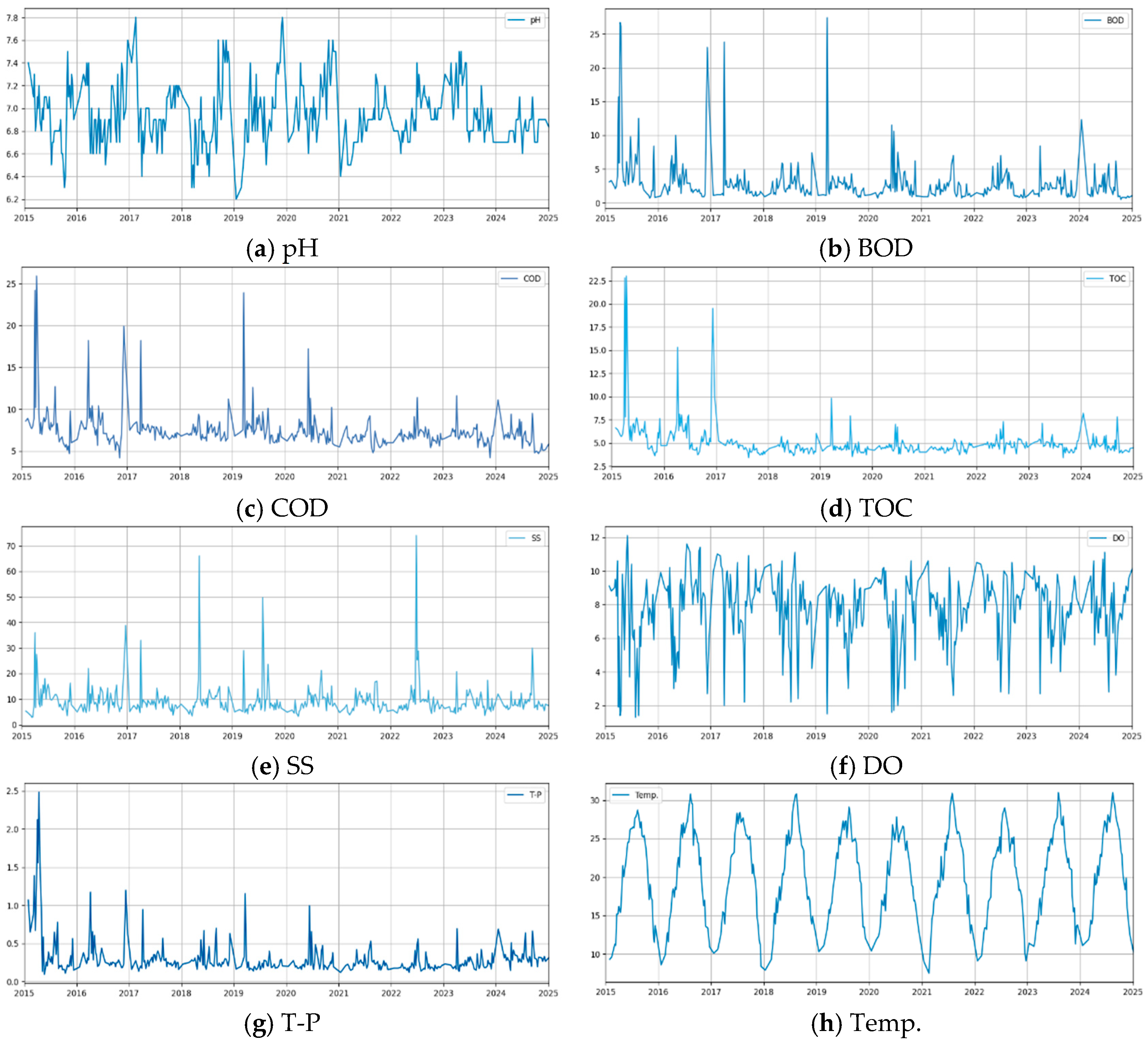
To support water quality improvement and management, the Ministry of Environment has established environmental standards for living environments [18]. Water quality is classified into the following grades: very good (Ia), good (Ib), slightly good (II), fair (III), slightly poor (IV), poor (V), and very poor (VI). Analysis showed that the average water quality of the Gulpocheon has remained relatively consistent over the past decade. The current status of major water quality indicators is presented in Figure 2 and Table 2.

2.2. Correlation Analysis

2.2.1. Pearson Correlation Coefficient Method

The Pearson correlation coefficient, introduced by Karl Pearson in 1895, is a statistical measure used to determine the linear relationship between two variables. The coefficient ranges from −1.0 to +1.0, where values close to +1 indicate a strong positive correlation and values close to −1 indicate a strong negative correlation. A coefficient near zero suggests that the two variables exhibit nonlinear behavior [19]. The coefficient is calculated using Equation (1), where C o v ( X , Y ) is the covariance of X and Y , σ X and σ Y are the standard deviations of X and Y , μ X and μ Y are their means, respectively, and N is the sample size.
ρ X , Y = C o v ( X , Y ) σ X σ Y = E [ ( X μ X ) ( Y μ Y ) ] σ X σ Y = i = 1 N ( X i μ X ) ( Y i μ Y ) σ X σ Y N

2.2.2. Principal Component Analysis

PCA is a statistical method that has been widely used since the 1930s to extract key information from complex datasets, particularly for dimensionality reduction [20]. When applied to correlation analysis of water quality indicators, PCA can interpret the interrelationships among parameters such as pH, COD, and DO, along with various chemical constituents. This enables the identification of principal variables that explain the largest variance within the dataset [21].

2.3. Machine Learning Algorithms

Machine learning algorithms were employed in this study to predict TOC concentrations. The selected models were the multilayer perceptron (MLP) and random forest (RF), both of which are effective in handling multivariate data and capturing nonlinear relationships among variables. All machine learning modeling was performed in Python 3.12.12.

2.3.1. Multilayer Perceptron (MLP)

The MLP model receives multiple water quality indicators (e.g., BOD, SS, T-N, T-P, EC, pH, temperature) at the input layer, where each input is weighted and biased before passing through an activation function into the hidden layers. Nodes within each hidden layer are fully connected to the nodes of the preceding layer, allowing the model to learn nonlinear interactions among variables. The abstracted features are progressively condensed through the hidden layers and aggregated at a single output node that produces the predicted TOC concentration. Predicted values are then compared with observed values to evaluate performance. The network is trained via backpropagation, enabling the multilayer structure to capture complex nonlinear relationships between water quality indicators and TOC [22].

2.3.2. Random Forest (RF)

The RF builds an ensemble of decision trees using bootstrap samples of the training data. Within each tree, at every split, the algorithm considers a random subset of predictors and selects the threshold that best reduces impurity. For instance, a first split might separate samples by whether COD exceeds a specified value, with later splits using other variables such as BOD or DO. This process yields increasingly homogeneous subsets, and each tree outputs a TOC prediction at its leaf nodes. The RF aggregates predictions by averaging across trees, with bootstrap sampling and feature subsetting reducing correlation among trees and improving generalization [23].

2.4. Exhaustive Search

Exhaustive search is a variable-selection procedure that enumerates all predictor subsets of pre-specified size and, for each subset, applies an identical training–evaluation protocol, then ranks subsets by performance metrics to identify the optimal set. Although this approach provides limited a priori physical or environmental justification for a given combination, it is valuable for systematically uncovering combinatorial effects that may not be captured by simple correlation screening and for interpreting selected sets in light of model structure in this study, excluding TOC, all combinations of 3–5 variables were generated from a pool of 15 candidate predictors (total of 4823 combinations), and each combination was trained and evaluated under an identical procedure using both MLP and RF models for comparison.

2.5. Grid Search

Grid search is a conventional approach for optimizing hyperparameters in machine learning models. It systematically explores all possible combinations of predefined hyperparameter sets to identify the optimal configuration. Although computationally expensive, this method provides robust performance gains and has been applied in various domains. Studies in medical and environmental data analysis have demonstrated that grid search–based hyperparameter optimization can significantly improve predictive accuracy [24,25,26]. Table 3 summarizes previous applications of grid search for hyperparameter optimization.

3. Results and Discussion

3.1. Correlation and Factor Analysis

To determine the input water quality parameters for TOC prediction models, we analyzed the correlations between TOC and other parameters. Two approaches were adopted: Pearson correlation analysis, which examines linear relationships between individual parameters, and PCA, which evaluates the combined influence of parameter groups on TOC variation. Correlation and principal component analyses were carried out exclusively on the training subset after the train–validation split. All analyses were performed using Python 3.12.12.
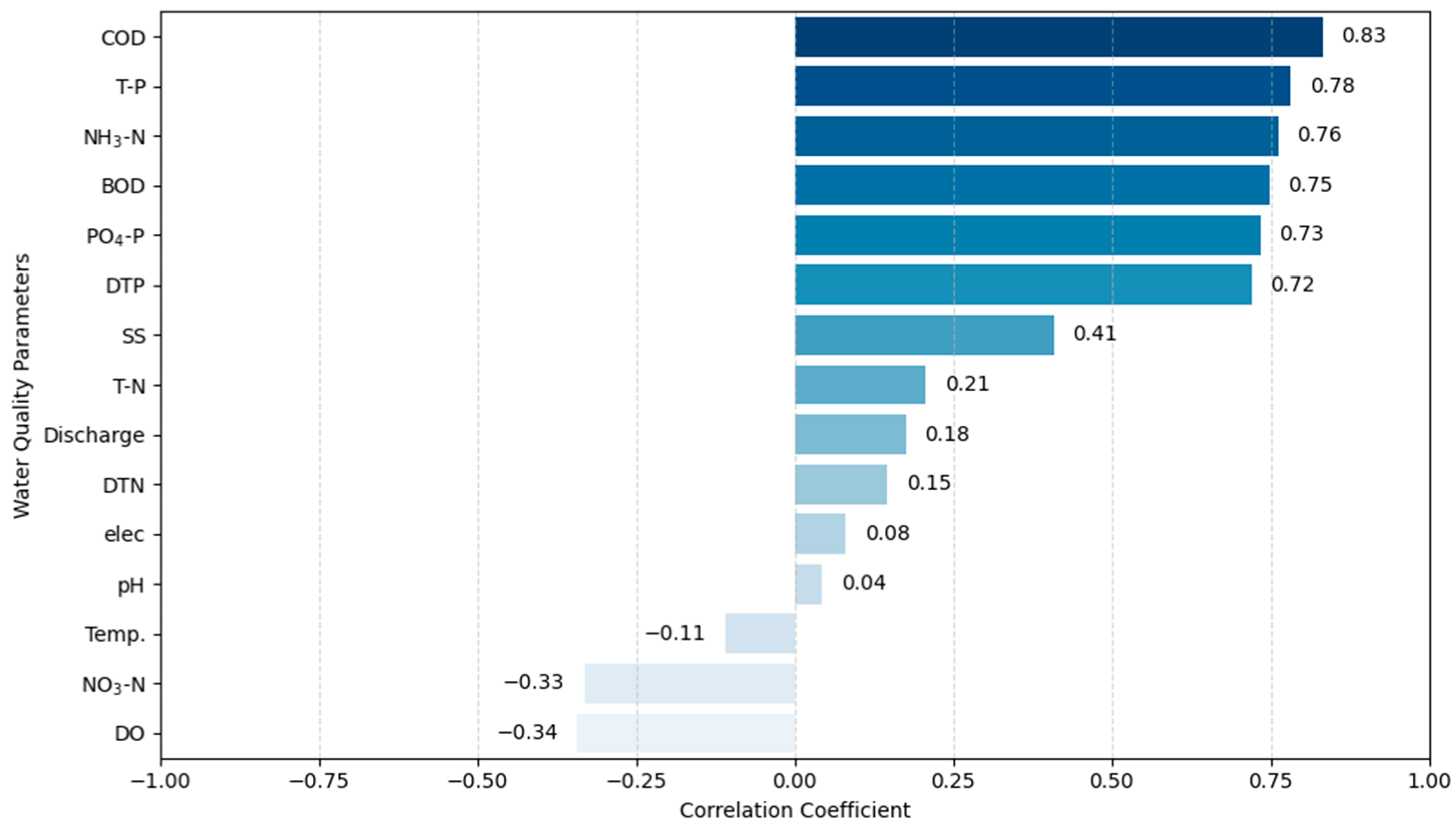
The results of the Pearson correlation analysis are shown in Figure 3.
COD (0.83), T-P (0.78), NH3-N (0.76), BOD (0.75), PO4-P (0.73), DTP (0.72), and SS (0.41) exhibited strong positive correlations with TOC, whereas DO (−0.34) and NO3-N (−0.33) showed strong negative correlations.
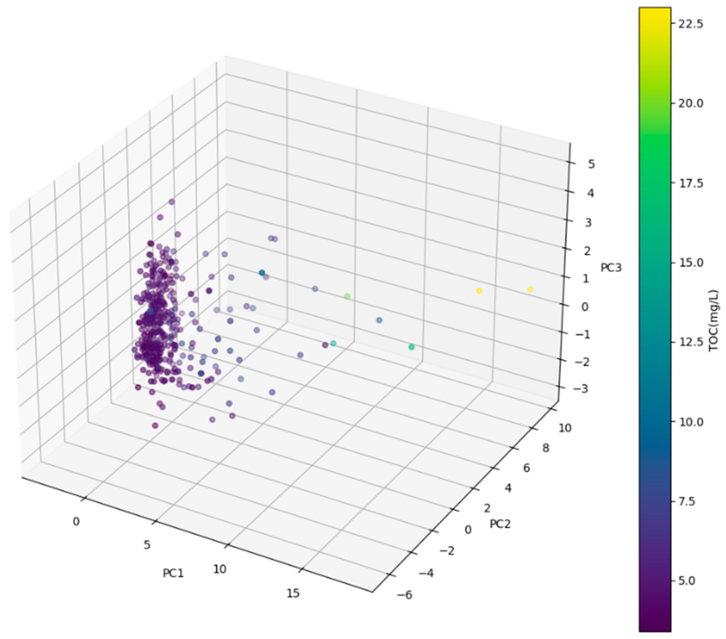
PCA was performed with three components to further examine the relationships between TOC and other water quality indicators, as presented in Figure 4.
Each axis (PC1, PC2, PC3) represents a principal component (PC), and each plotted point corresponds to a parameter. Clusters of points within the PCA space indicate parameters with similar characteristics.
The analysis revealed that most parameters tended to cluster within a specific region of the PCA space, suggesting that TOC and other indicators shared common patterns of variation. When TOC concentrations were below approximately 10 mg/L, strong correlations with other parameters were observed, whereas concentrations above this threshold showed a tendency to diverge from the clustered group. The explained variance and loadings of each principal component are listed in Table 4.
PC1 explained 41% of the total variance and showed positive loadings for BOD (0.341), COD (0.327), T-P (0.340), NH3-N (0.346), Dissolved total phosphorus (DTP) (0.316), Orthophosphate as phosphorus (PO4-P) (0.313), and SS (0.253), whereas DO (−0.302) and NO3-N (−0.302) had negative loadings. PC2 exhibited high positive loadings for T-N (0.493), Dissolved total nitrogen (DTN) (0.453), EC (0.378), and NO3-N (0.278). PC3 was dominated by pH (0.836), with positive contributions from SS (0.306) and DO (0.205), and a negative contribution from temperature (−0.302).
PC1 can be interpreted as a combined axis of organic pollution (BOD, COD), nutrient enrichment (NH3-N, T-P, phosphate series), and oxygen depletion (negative DO), representing a general nutrient and organic pollution gradient. These results were consistent with findings from previous PCA studies (Table 5).
To evaluate the relative influence of each water quality parameter on TOC variation, we weighted the loadings of individual parameters using the explained variance of each principal component, as defined in Equation (2). L o a d i n g i , P C k denotes the loading value of variable i on P C k , and E x p l . V a r P C k represents the proportion of variance explained by P C k .
Influence ( x i ) = k = 1 m ( L o a d i n g i , P C k × E x p l . V a r P C k )
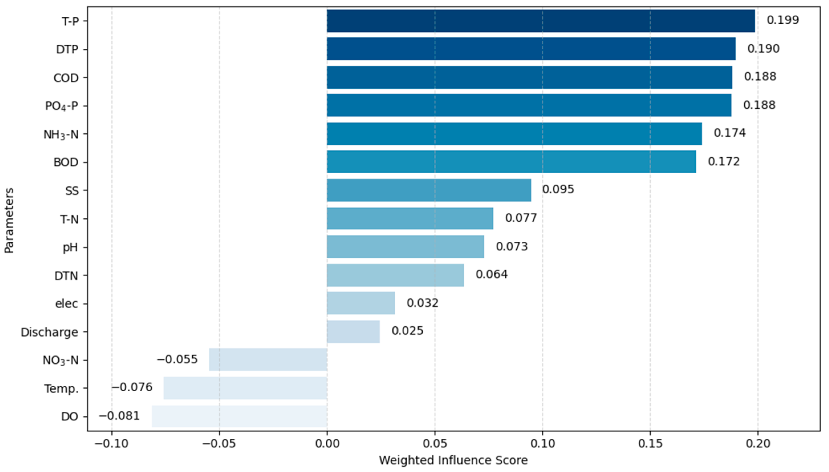
The weighted influence analysis results are presented in Figure 5. Parameters with the strongest positive influence were T-P (0.199), DTP (0.190), COD (0.188), PO4-P (0.188), NH3-N (0.174), and BOD (0.172), indicating that nutrient- and organic-related indicators were the primary contributors to TOC variability.

3.2. Development of TOC Prediction Models

To identify combinations of water quality parameters that yield higher predictive performance beyond those selected by Pearson correlation and PCA, we conducted an exhaustive search. Combinations of three to five water quality parameters were tested. In the initial analysis, the hyperparameters of each machine learning model were set to their default values, and the configurations are presented in Table 6.
Prior to model training, all predictor variables were standardized using the z-score transformation. To preserve temporal dependence, the data were split chronologically into training and test sets at an 8:2 ratio. Standardization statistics (mean and standard deviation) were computed on the training set only, and the same transformation was applied to the test set to prevent data leakage [29].
Although the data were collected in chronological order, during model training each timestamp was treated as an independent sample, and TOC was predicted from the relationships among the concurrently observed water quality variables.
The results of the exhaustive search for the MLP model are summarized in Table 7. Predictive performance was evaluated using R2 (coefficient of determination), RMSE (root mean squared error), and MAE (mean absolute error). The best-performing combination consisted of DO, COD, T-P, DTP, and PO4-P, achieving an R2 of 0.7496, an RMSE of 0.3946, and an MAE of 0.2921. The top three combinations consistently included DO, COD, T-P, and PO4-P, demonstrating their importance as predictive variables. Notably, COD was included in all of the top ten combinations, while DO and T-P appeared in eight of them.
The results for the RF model are presented in Table 8. The highest predictive performance was achieved using temperature, BOD, COD, SS, and discharge as input variables, with an R2 of 0.6788, an RMSE of 0.4470, and an MAE of 0.3376. Among the top five combinations, temperature, BOD, and COD appeared consistently, indicating their strong contributions to TOC prediction. COD was included in all of the top ten combinations, consistent with the MLP results.
Considering the input subsets yielding higher accuracy by model, the MLP tended to select DO, whereas the RF tended to select Temperature. Because DO is a composite indicator in which seasonality and biogeochemical processes are superimposed, its relationship with TOC is likely nonlinear and interaction-driven. The MLP is well suited to capture such nonlinear combinations and may therefore have leveraged the DO signal more effectively. In contrast, RF selects, at each split, the partition that maximizes impurity reduction among a randomly chosen subset of predictors; consequently, a variable with a strong univariate (seasonal) signal such as Temperature can be repeatedly used near the top of trees and accumulate higher importance.
Accordingly, collinearity between Temperature and DO may bias importance attribution toward one variable, so in this dataset Temperature appears more influential for RF, whereas DO appears more influential for MLP.
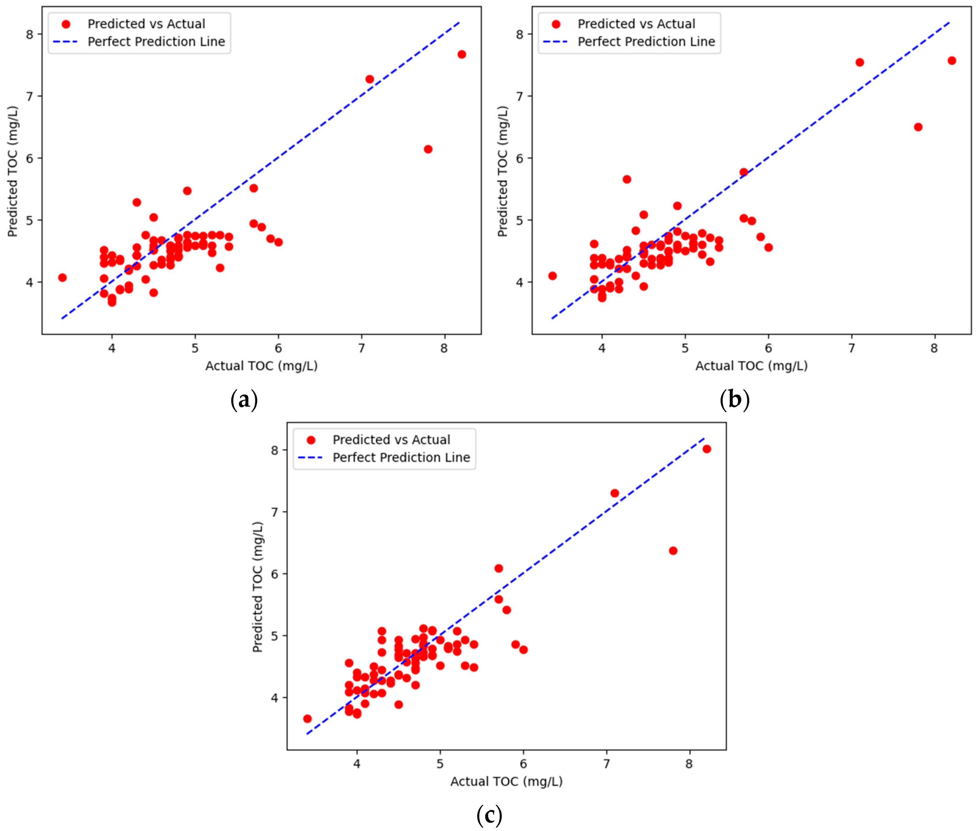
TOC prediction results using the MLP, with input water quality variables derived from exhaustive search and correlation analysis, are shown in Figure 6 and Table 9.
In Figure 6a, when the TOC prediction model used the top five parameters that showed strong positive correlations with TOC in the Pearson correlation analysis (BOD, COD, T-P, NH3-N, and PO4-P), the model achieved an R2 of 0.6150, RMSE of 0.4893 and MAE of 0.3752.
As shown in Figure 6b, when the model used the top five parameters identified by PCA (COD, T-P, NH3-N, DTP, and PO4-P), the results showed an R2 of 0.6118, RMSE of 0.4913 and MAE of 0.3804.
As shown in Figure 6c, the prediction model achieved the highest performance when using the parameters identified through exhaustive search (DO, COD, T-P, DTP, and PO4-P), yielding an R2 of 0.7496, RMSE of 0.3946 and MAE of 0.2921. Compared with the models using input variables selected by Pearson correlation analysis and PCA, the exhaustive search approach improved predictive accuracy by approximately 22%.
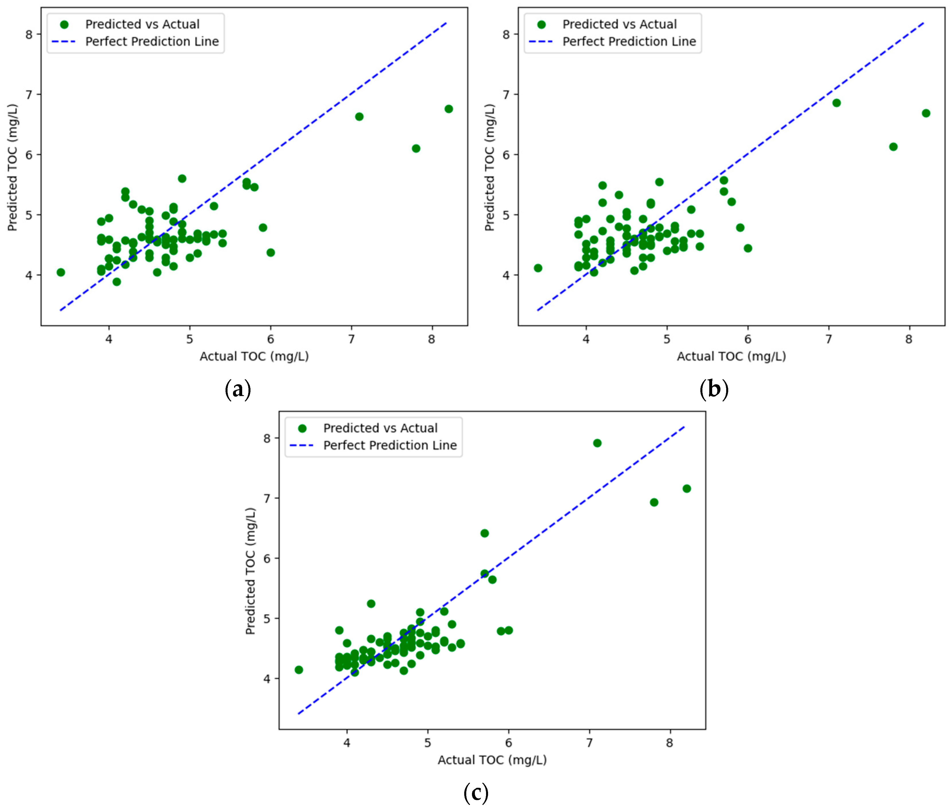
Figure 7 and Table 10 present the results of TOC prediction using the RF model.
As shown in Figure 7a, the TOC prediction model using the top five parameters that showed strong positive correlations with TOC in the Pearson correlation analysis (BOD, COD, T-P, NH3-N, and PO4-P) yielded an R2 of 0.4774, RMSE of 0.5701 and MAE of 0.4421.
As shown in Figure 7b, the TOC prediction model using the top five parameters identified by PCA (COD, T-P, NH3-N, DTP, and PO4-P) produced an R2 of 0.4574, RMSE of 0.5809 and MAE of 0.4484.
Figure 7c shows the results when the input parameters selected through exhaustive search (Temp., BOD, COD, SS, and discharge) were applied. This combination achieved the highest prediction performance, with an R2 of 0.6788, RMSE of 0.4470 and MAE of 0.3376. Compared with the models using variables selected by Pearson correlation and PCA, exhaustive search improved prediction accuracy by approximately 45%.
Overall, TOC prediction using machine learning demonstrated that the MLP model outperformed the RF model by an average of about 20%. Moreover, when input variables were selected through exhaustive search rather than solely through correlation-based or PCA-based methods, prediction performance improved by more than 20% in both the MLP and RF models.

3.3. Hyperparameter Tuning of TOC Prediction Models

To further improve the performance of the TOC prediction models, we optimized hyperparameters of the machine learning algorithms and compared the results. Hyperparameter tuning was conducted for both the MLP and RF models, using as input variables that the parameter sets identified through exhaustive search.
For the MLP model, the baseline configuration consisted of a single hidden layer with 100 neurons, relu activation, and an initial learning rate of 0.001, a regularization strength (alpha) of 0.0001. Grid search was applied to evaluate performance improvements under different parameter settings, with the search space listed in Table 11.
In this context, hidden_layer_sizes specifies the number of hidden layers and neurons; activation defines the activation function, relu indicates a rectified linear function, and tanh indicates a hyperbolic function. The parameter alpha represents the strength of L2 regularization, which constrains the magnitude of weights to mitigate overfitting. Smaller values reduce the constraint and increase sensitivity to fluctuations in the data, but at the cost of higher overfitting risk. learning_rate_init determines the speed of weight updates, where larger values accelerate convergence but may overshoot the optimum or destabilize training.
For the RF model, the baseline configuration employed 100 trees with no maximum depth constraint, requiring at least two samples to split an internal node and one sample at each leaf node. The set of values analyzed to determine the optimal hyperparameter configuration for the RF model is presented in Table 12.
In this context, the key hyperparameters examined included n_estimators, max_depth, min_samples_split, and min_samples_leaf. Increasing the number of trees generally stabilizes performance but prolongs computation. A deeper max_depth enables more complex tree structures, improving fit but risking overfitting. Higher values of min_samples_split make the model more conservative by requiring more samples at each split, whereas min_samples_leaf controls the minimum samples required at leaf nodes.
Table 13 compares baseline and optimized performances. For the MLP, R2 improved from 0.7496 to 0.7562 (~0.9%) with one hidden layer of 100 neurons, ReLU activation, alpha = 0.001, and an initial learning rate of 0.003. For the RF, R2 increased from 0.6788 to 0.7058 (~4.0%) using 100 trees, unlimited maximum depth, min_samples_split = 10, and min_samples_leaf = 1.
Additionally, following hyperparameter tuning, the reduction in MAE indicates a decrease in the typical (average) prediction error, whereas the reduction in RMSE suggests a contraction of the overall error distribution, including large deviations. Collectively, these results demonstrate that tuning yielded modest yet consistent enhancements in generalization performance and model stability for both the MLP and RF models.
The most influential hyperparameters were alpha, learning_rate_init, and min_samples_split, all related to model regularization. In the MLP model, a larger alpha constrained the weight magnitudes, reducing sensitivity to noise. A higher learning_rate_init accelerated convergence and improved training efficiency. In the RF model, increasing min_samples_split reduced the number of splits, creating a more conservative structure.
By strengthening regularization, streamlining the training process, and designing more conservative models, the prediction accuracy improved. This is attributed to the characteristics of the study site, Gulpocheon, which is a highly variable urban stream subject to diverse nonpoint sources such as stormwater runoff, construction, and domestic sewage. The TOC time series data are therefore characterized by substantial variability and noise. Without adequate regularization, the models risk overfitting to short-term fluctuations and noise. With stronger regularization, models became less sensitive to anomalies, focusing instead on long-term patterns and average relationships. As a result, generalization performance improved and prediction accuracy for validation data increased.

4. Conclusions

This study developed TOC prediction models for the Gulpocheon watershed using diverse water quality parameters and compared prediction performance according to variable selection methods and hyperparameter tuning. The main findings are summarized as follows.
First, Pearson correlation and principal component analyses indicated that COD, T-P, NH3-N, DTP, PO4-P, and BOD exhibited strong correlations with TOC. In particular, PC1 was interpreted as an axis combining organic indicators (BOD, COD), nutrient indicators (NH3-N, T-P, phosphate series), and the negative association with DO, confirming their dominant contribution to TOC variability.
Second, exhaustive search revealed that variable selection solely based on correlation analysis had limitations in securing prediction accuracy. Even parameters with relatively weak direct correlations with TOC achieved higher predictive performance when combined in specific sets. This result highlights the importance of identifying optimal combinations of input variables to enhance model accuracy, consistent with the findings of Ju et al. [30], who reported that models relying only on Pearson-selected factors yielded lower accuracy compared with those using exhaustive search-derived combinations.
Third, exhaustive search revealed model-specific input preferences: the MLP primarily selected DO, whereas the RF primarily selected Temperature. This pattern likely reflects DO’s nonlinear/interaction-rich signal, the split-by-impurity structure of RF, and Temperature–DO collinearity, confirming model-specific contributions of DO/Temperature alongside COD in this study.
Fourth, in baseline predictions without hyperparameter tuning, the MLP model consistently outperformed the RF model, showing on average 20% higher predictive power. COD was included in all top-performing combinations, confirming its role as the most critical input variable.
Fifth, hyperparameter tuning improved model performance, increasing R2 from 0.7496 to 0.7562 for the MLP model and from 0.6788 to 0.7058 for the RF model. Key parameters adjusted (alpha, learning_rate_init, and min_samples_split) were all related to regularization. Strengthening model regularization and adopting more conservative training strategies reduced sensitivity to noise and short-term fluctuations, thereby enhancing generalization and predictive accuracy.
Combining an exhaustive exploration of input-variable combinations with regularization-oriented hyperparameter tuning can meaningfully improve the generalization and predictive performance of TOC models. The Gulpocheon constitutes a managed urban stream exhibiting high variability due to diverse nonpoint sources (e.g., stormwater runoff, construction-related discharge, domestic sewage) and dilution/mixing associated with reclaimed-water inflow. Within this context, an input-variable design framework tailored to managed streams was established, and predictive performance was evaluated through an exhaustive search of variable combinations.
The proposed modeling approach appears potentially applicable to other streams receiving reclaimed water under conditions similar to those of the study area. For basins with different hydro-environmental regimes, the framework—exhaustive identification of input variables followed by regularization-enhanced hyperparameter tuning—may enable the development of high-accuracy predictive models, although additional validation is warranted.

Author Contributions

Conceptualization, K.B.J. and D.W.J.; methodology, K.B.J. and D.W.J.; software, K.B.J.; validation, K.B.J. and D.W.J.; formal analysis, K.B.J.; investigation, K.B.J.; resources, K.B.J.; writing—original draft preparation, K.B.J.; writing—review and editing, D.W.J.; visualization, K.B.J.; supervision, D.W.J. All authors have read and agreed to the published version of the manuscript.

Funding

This work was supported by Korea Water Cluster through 2024 Project for Active and Digitalization of Water Technology (202402-0201).

Data Availability Statement

The original contributions presented in this study are included in the article. Further inquiries can be directed to the corresponding author.

Acknowledgments

The authors appreciate the support from Korea Water Cluster.

Conflicts of Interest

The authors declare no conflict of interest.

References

  1. Amarasinghe, H.A.U.; Gunawardena, H.D.; Jayatunga, Y.A. Correlation between biochemical oxygen demand (BOD) and chemical oxygen demand (COD) for different industrial waste waters. J. Natl. Sci. Found. Sri Lanka 1993, 21, 259–266. [Google Scholar] [CrossRef]
  2. Rudaru, D.G.; Lucaciu, I.E.; Fulgheci, A.M. Correlation between BOD5 and COD—Biodegradability indicator of wastewater. Rom. J. Ecol. Environ. Chem. 2022, 4, 80–86. [Google Scholar] [CrossRef]
  3. Alewi, H.K.; Abood, E.A.; Ali, G. An inquiry into the relationships between BOD5, COD, and TOC in Tigris River, Maysan Province, Iraq. Casp. J. Environ. Sci. 2022, 20, 37–43. [Google Scholar] [CrossRef]
  4. Choi, I.W.; Kim, J.H.; Im, J.K.; Park, T.J.; Kim, S.Y.; Son, D.H.; Huh, I.A.; Rhew, D.H.; Yu, S.J. Application of TOC standards for managing refractory organic compounds in industrial wastewater. J. Korean Soc. Water Environ. 2015, 31, 29–34. [Google Scholar] [CrossRef]
  5. ES 04316.1a; Dissolved Organic Carbon—High Temperature Combustion Method. National Institute of Environmental Research (NIER): Incheon, Republic of Korea, 2024.
  6. ES 04316.2a; Dissolved Organic Carbon—Persulfate-Ultraviolet or Heated-Persulfate Oxidation Method. National Institute of Environmental Research (NIER): Incheon, Republic of Korea, 2024.
  7. Yoon, S.B.; Lee, C.H.; Kim, Y.D. Development of a real-time TOC estimation model using spectroscopic data and machine learning techniques. J. Water Environ. Technol. 2023, 56, 815–822. [Google Scholar] [CrossRef]
  8. Kokya, T.A.; Mehrdadi, N.; Ardestani, M.; Baghvand, A.; Kazemi, A.; Kalhori, A.A.M. Intelligent multivariate model for the optical detection of total organic carbon. J. Chil. Chem. Soc. 2016, 61, 3055–3060. [Google Scholar] [CrossRef]
  9. Kim, C.; Eom, J.B.; Jung, S.; Ji, T. Detection of Organic Compounds in Water by an Optical Absorbance Method. Sensors. 2016, 16, 61. [Google Scholar] [CrossRef]
  10. Guo, H.; Song, Y.; Tang, H.; Zhao, J. An ensemble deep neural network approach for predicting TOC concentration in lakes along the middle-lower reaches of Yangtze River. J. Intell. Fuzzy Syst. 2022, 42, 1455–1482. [Google Scholar] [CrossRef]
  11. Oh, H.; Park, H.Y.; Kim, J.I.; Lee, B.J.; Choi, J.H.; Hur, J. Enhancing machine learning models for total organic carbon prediction by integrating geospatial parameters in river watersheds. Sci. Total Environ. 2024, 943, 173743. [Google Scholar] [CrossRef]
  12. Kemei, E.K.; Van Laerhoven, K.; Karuri, N.W.; Kimutai, R. Multivariate prediction of total organic carbon in river water using random forest and deep learning regression algorithms. Appl. Comput. Intell. 2025, 5, 264–285. [Google Scholar] [CrossRef]
  13. Tomperi, J.; Isokangas, A.; Ruusunen, M. Practical data-based modelling approach for estimating river water turbidity and total organic carbon. Environ. Technol. 2025, 46, 4624–4640. [Google Scholar] [CrossRef]
  14. Goz, E.; Yuceer, M.; Karadurmus, E. Total organic carbon prediction with artificial intelligence techniques. In Computer Aided Chemical Engineering; Elsevier: Amsterdam, The Netherlands, 2019; Volume 46, pp. 889–894. [Google Scholar] [CrossRef]
  15. Nafsin, N.; Li, J. Prediction of total organic carbon and E. coli in rivers within the Milwaukee River basin using machine learning methods. Environ. Sci. Adv. 2023, 2, 278–293. [Google Scholar] [CrossRef]
  16. Jang, D. Analysis of the water quality improvement in urban Stream using MIKE 21 FM. Appl. Sci. 2021, 11, 8890. [Google Scholar] [CrossRef]
  17. Ministry of the Environment. Ecological River Restoration Guidebook; Ministry of the Environment: Sejong City, Republic of Korea, 2011.
  18. Ministry of Environment. Enforcement Decree of the Framework Act on Environmental Policy. Available online: https://elaw.klri.re.kr/kor_service/lawView.do?hseq=63038&lang=eng (accessed on 3 November 2025).
  19. Jung, J.-M.; Park, S.-H.; Lee, Y.-S.; Gim, J.-H. The development of infrared thermal imaging safety diagnosis system using Pearson’s correlation coefficient. J. Korean Sol. Energy Soc. 2019, 39, 55–65. [Google Scholar] [CrossRef]
  20. Nguyen, T.H.; Helm, B.; Hettiarachchi, H.; Caucci, S.; Krebs, P. Quantifying the Information Content of a Water Quality Monitoring Network Using Principal Component Analysis: A Case Study of the Freiberger Mulde River Basin, Germany. Water 2020, 12, 420. [Google Scholar] [CrossRef]
  21. Huda, N.; Ahmed, T.; Masum, M.H.; Faruque, N.; Islam, M.S. Assessment of surface water quality using advanced statistical techniques around an urban landfill: A multi-parameter analysis. City Environ. Interact. 2025, 28, 100237. [Google Scholar] [CrossRef]
  22. Rumelhart, D.; Hinton, G.; Williams, R. Learning representations by back-propagating errors. Nature 1986, 323, 533–536. [Google Scholar] [CrossRef]
  23. Breiman, L. Random forests. Mach. Learn. 2001, 45, 5–32. [Google Scholar] [CrossRef]
  24. Hashi, E.K.; Zaman, M.S.U. Developing a hyperparameter tuning based machine learning approach of heart disease prediction. J. Appl. Sci. Process Eng. 2020, 7, 631–647. [Google Scholar] [CrossRef]
  25. Anil, N.; Ram, A.; Krishnan, M.S. Water quality analysis of canals using machine learning algorithms and hyperparameter turning. In Proceedings of the 4th International Conference on Computing Communication and Networking Technologies (ICCCNT), New Delhi, India, 6–8 July 2023; IEEE: New York, NY, USA, 2023; pp. 1–5. [Google Scholar] [CrossRef]
  26. Elvin, E.; Wibowo, A. Forecasting water quality through machine learning and hyperparameter optimization. Indones. J. Electr. Eng. Comput. Sci. 2024, 33, 496–506. [Google Scholar] [CrossRef]
  27. Le, T.T.H.; Zeunert, S.; Lorenz, M.; Meon, G. Multivariate statistical assessment of a polluted river under nitrification inhibition in the tropics. Environ. Sci. Pollut. Res. Int. 2017, 24, 13845–13862. [Google Scholar] [CrossRef] [PubMed]
  28. Doan, V.T.; Le, C.C.; Le, H.V.T.; Trieu, N.A.; Vo, P.L.; Tran, D.A.; Nguyen, H.V.; Tabata, T.; Vu, T.T.H. Comprehensive Statistical Analysis for Characterizing Water Quality Assessment in the Mekong Delta: Trends, Variability, and Key Influencing Factors. Sustainability 2025, 17, 5375. [Google Scholar] [CrossRef]
  29. Scikit-Learn Developers. 11.2 Data Leakage—Common Pitfalls and Recommended Practices. Available online: https://scikit-learn.org/stable/common_pitfalls.html (accessed on 3 November 2025).
  30. Ju, K.B.; Jung, H.N.; Jang, D.W. Selection of optimal water quality parameters and model for TOC concentration estimation. Crisisonomy 2025, 21, 143–159. [Google Scholar] [CrossRef]
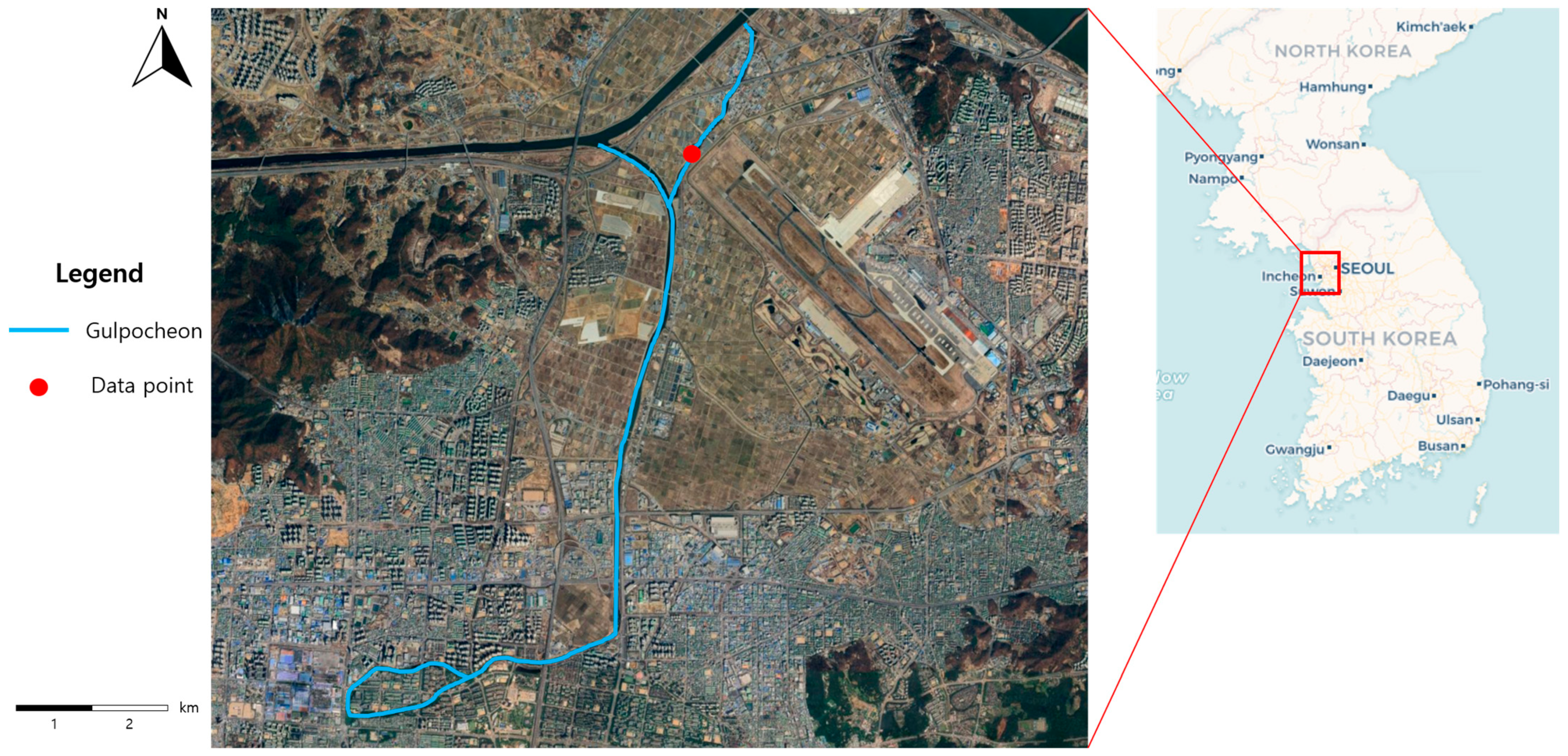
Figure 1. Location of the Gulpocheon and water quality monitoring site.
Water 17 03367 g001
Figure 2. Ten-year temporal dynamics of key water quality indicators (pH, BOD, COD, TOC, SS, DO, T-P, Temp.) in the Gulpocheon.
Water 17 03367 g002
Figure 3. Pearson correlations (r) between TOC and other water quality parameters in the Gulpocheon (bars show −1 to +1).
Water 17 03367 g003
Figure 4. Three-dimensional PCA score plot (PC1–PC3) of water quality samples from the Gulpocheon; points denote observations and color indicates TOC.
Water 17 03367 g004
Figure 5. Weighted influence scores of water quality parameters on TOC in the Gulpocheon.
Water 17 03367 g005
Figure 6. Comparison of TOC prediction performance according to input feature selection strategies (MLP): (a) Pearson correlation, (b) PCA, (c) Exhaustive search. The x-axis denotes measured TOC (mg L−1) and the y-axis denotes predicted TOC (mg L−1); red circles represent prediction–observation pairs, and the blue dashed line indicates the 1:1 reference (y = x).
Water 17 03367 g006
Figure 7. Comparison of TOC prediction performance according to input feature selection strategies (RF): (a) Pearson correlation, (b) PCA, (c) Exhaustive search.
Water 17 03367 g007
Table 1. Summary of previous studies on TOC prediction using water quality parameters.
AuthorSiteFeaturesPrediction Methods
Guo et al., 2022 [10]Yangtze RiverTemp., pH, DO, EC, Chl-a, NH4DNN
Oh et al., 2024 [11]Geumho RiverpH, DO, EC, T-N, T-P, Turbidity, Temp., Discharge, Land Use, Slope, Flow RateXGBoost, DNN, MLR
Kemei et al., 2025 [12]Duwamish RiverDepth, Density, DOC, Light Transmissivity, PO4-P, Silica, TSS, Salinity, DateRF, CNN, MLP
Tomperi et al., 2025 [13]Southern FinlandWater Temperature,
Water level
MLR, PLSR, NN
Goz et al., 2019 [14]Yeşilırmak RiverpH, Conductivity, Dissolved Oxygen, Temp.ELM, KELM, ANN, PLSR
Nafsin & Li 2023 [15]Milwaukee RiverBOD, EC, Cl, NO3, VSS, DO, Turbidity, pH, TSSANN, SVM, RF, GBM
Notes: Temp.—Temperature; pH—pH; DO—Dissolved Oxygen; EC—Electrical Conductivity; Chl-a—Chlorophyll-a; NH4—Ammonium; DNN—Deep Neural Network; T-N—Total Nitrogen; T-P—Total Phosphorus; XGBoost—Extreme Gradient Boosting; MLR—Multiple Linear Regression; DOC—Dissolved Organic Carbon; PO4-P—Orthophosphate; TSS—Total Suspended Solids; RF—Random Forest; CNN—Convolutional Neural Network; MLP—Multilayer Perceptron; PLSR—Partial Least Squares Regression; NN—Neural Network; ELM—Extreme Learning Machine; KELM—Kernel Extreme Learning Machine; ANN—Artificial Neural Network; BOD—Biochemical Oxygen Demand; Cl—Chloride; NO3—Nitrate; VSS—Volatile Suspended Solids; SVM—Support Vector Machine; GBM—Gradient Boosting Machine.
Table 2. Period-specific water quality status of the Gulpocheon River by national environmental standards.
CategorypHBOD
(mg/L)
COD
(mg/L)
TOC
(mg/L)
SS
(mg/L)
DO
(mg/L)
T-P
(mg/L)
10 yearsAverage6.942.67.254.819.307.840.27
GradeIaIIIVIIIIaIaIV
5 yearsAverage6.902.186.704.729.057.850.26
GradeIaIIIVIIIIaIaIV
1 yearAverage6.81.26.24.57.110.40.34
GradeIaIbIVIIIIaIaIV
Table 3. Summary of previous studies using grid search for hyperparameter tuning.
StudyApplication AreaModels UsedKey Tuned
Hyperparameters
Performance Improvement
Hashi & Zaman, 2020 [24]Heart disease predictionLR, KNN, SVM, DT, RFC, gamma, solver, max_depth, etc.LR: 88.52% → 90.16%
KNN: 90.16% → 91.80%
SVM: 88.52% → 90.16%
DT: 81.97% → 86.89%
Anil et al., 2023 [25]Canal water quality predictionRFn_estimators, max_depth, min_samples_split, min_samples_leaf, max_featuresCV score: 0.92 → 0.94
Elvin & Wibowo, 2024 [26]Water quality forecasting (multiple ML models)XGBoost, RF, DT, Adaptive Boosting, SVM, Naive Bayes,
Extra Tree
Model-specific tuned parametersSVM: 78% → 90.06%
XGBoost: 96.93% → 97.06%
DT: 95% → 95.69%
Notes: LR—Linear Regression; KNN—k-Nearest Neighbors; SVM—Support Vector Machine; DT—Decision Tree; RF—Random Forest; CV—Cross-Validation.
Table 4. Principal component loadings (PC1–PC3) for major water quality variables in the Gulpocheon.
VariablePC1PC2PC3
Variance ratio0.41340.26530.0784
Temp.0.0797−0.3201−0.3017
DO−0.30170.10260.2049
BOD0.34110.1610−0.0037
COD0.32660.18570.0503
SS0.2534−0.12780.3059
T-N−0.08520.4931−0.1198
T-P0.33990.21690.0135
pH0.00780.01510.8363
EC−0.16480.3783−0.0082
DTN−0.11270.4525−0.1235
NH3-N0.34630.1389−0.0788
NO3-N−0.30150.27800.0472
DTP0.31620.22240.0001
PO4-P0.31290.20760.0152
Discharge0.2012−0.1661−0.1836
Table 5. Summary of PC (explained variance and axis interpretation) in different studies.
StudyPC (Explained Variance, %)Major Loading VariablesAxis
This studyPC1 (41.3%)BOD, COD, T-P, NH3-N, DTP, PO4-P, DO, NO3-NNutrient pollution and organic pollution axis
Le et al., 2017 [27]PC1 (27.1%)Conductivity, NH4-N, PO4-P, T-PNutrient pollution
PC2 (22.2%)BOD5, COD, NorgOrganic pollution
Doan et al., 2025 [28]PC1 (23.1%)BOD5, COD, TOC, CdOrganic pollution
Table 6. Default hyperparameters for the MLP and Random Forest models.
MLPactivationalphalearning_rate_inithidden layer
relu0.00010.001(100)
RFn_estimatorsmax_depthmin_samples_splitmin_samples_leaf
100none21
Table 7. Evaluation of top 10 feature combinations for TOC prediction using MLP.
RankFeaturesR2RMSEMAE
1DO, COD, T-P, DTP, PO4-P0.74960.39460.2921
2DO, COD, T-P, NO3-N, PO4-P0.73530.40570.2933
3DO, COD, T-P, pH, PO4-P0.72890.41060.3065
4COD, SS, DTN0.72280.41520.3054
5DO, COD, T-P0.72190.41590.3132
6DO, COD, T-P, NO3-N, DTP0.71910.41790.3062
7DO, COD, SS, T-P, PO4-P0.71840.41850.3021
8COD, SS, T-N0.71680.41970.3129
9DO, BOD, COD, T-P, PO4-P0.71610.42020.3022
10DO, COD, SS, T-N, T-P0.71400.42180.3134
Table 8. Evaluation of top 10 feature combinations for TOC prediction using RF.
RankFeaturesR2RMSEMAE
1Temp., BOD, COD, SS, Discharge0.67880.44700.3376
2Temp., BOD, COD, SS, DTP0.65280.46470.3511
3Temp., BOD, COD, SS, NH3-N0.65100.46590.3578
4Temp., BOD, COD0.64830.46770.3367
5Temp., DO, BOD, COD0.64140.47230.3752
6DO, BOD, COD, SS, Discharge0.63780.47460.3424
7BOD, COD, SS, pH, Discharge0.63520.47630.3693
8Temp., BOD, COD, T-P, DTP0.62960.48000.3606
9Temp., DO, BOD, COD, Discharge0.62790.48110.3723
10Temp., COD, SS, NH3-N0.62730.48140.3651
Table 9. TOC prediction accuracy using MLP by feature selection strategy, with selected input features.
MethodFeatureR2RMSEMAE
Pearson correlationBOD, COD, T-P, NH3-N, PO4-P0.61500.48930.3752
PCACOD, T-P, NH3-N, DTP, PO4-P0.61180.49130.3804
Exhaustive searchDO, COD, T-P, DTP, PO4-P0.74960.39460.2921
Table 10. TOC prediction accuracy using RF by feature selection strategy, with selected input features.
MethodFeatureR2RMSEMAE
Pearson correlationBOD, COD, T-P, NH3-N, PO4-P0.47740.57010.4421
PCACOD, T-P, NH3-N, DTP, PO4-P0.45740.58090.4484
Exhaustive searchTemp., BOD, COD, SS, Discharge0.67880.44700.3376
Table 11. Hyperparameter search space for the MLP model in grid search.
ParameterSearch Values List
hidden_layer_sizes(100), (100, 50), (100, 100), (100, 50, 50), (100, 100, 50)
activation‘relu’, ‘tanh’
alpha0.0001, 0.001, 0.00001, 0.0005
learning_rate_init0.001, 0.003, 0.0005, 0.0001
Table 12. Hyperparameter search space for the RF model in grid search.
ParameterSearch Values List
n_estimators100, 200, 300, 400, 500
max_depthnone, 6, 8, 10, 12
min_samples_split2, 5, 10
min_samples_leaf1, 2, 4
Table 13. Comparison of Default and optimized hyperparameters with model performance (R2).
ModelDefault HyperparametersR2
RMSE
MAE
Optimized
Hyperparameters
R2
RMSE
MAE
MLPalpha0.00010.7496
0.3946
0.2921
alpha0.0010.7562
0.3894
0.2822
activationreluactivationrelu
learning_rate_init0.001learning_rate_init0.003
hidden layer(100)hidden layer(100)
RFn_estimators1000.6788
0.4470
0.3376
n_estimators1000.7058
0.4278
0.3212
max_depthnonemax_depthnone
min_samples_split2min_samples_split10
min_samples_leaf1min_samples_leaf1
Disclaimer/Publisher’s Note: The statements, opinions and data contained in all publications are solely those of the individual author(s) and contributor(s) and not of MDPI and/or the editor(s). MDPI and/or the editor(s) disclaim responsibility for any injury to people or property resulting from any ideas, methods, instructions or products referred to in the content.