Designing an Optimal Environmental Policy for Omura Bay, Japan: A Simulation Study on Water Quality Improvements

Abstract

This study aimed to explore the trade-offs between regional economic activity and environmental policy to explore economic approaches for reducing and managing pollutant discharge while maintaining a balance between socioeconomic activities and the marine environment. A linear programming simulation was conducted to model the interactions between socioeconomic activities, pollutant emissions, and reduction policies in the Omura Bay watershed. The model was designed to maximize Gross Regional Product (GRP), using inflow pollutant loads as a constraint. The simulation showed that a 12.7% reduction in 2015 pollutant loads is feasible under total load control. However, this level of reduction would cause a 14% decrease in watershed GRP. Further analysis revealed that reductions beyond 12.4% would significantly lower GRP and increase the cost of mitigation, making a 12.3% reduction the most realistic upper limit. The estimated cost of implementing countermeasures to manage pollutant inflow was JPY 6.7 billion, which would translate to a JPY 37.6 billion reduction in the cost to maintain current conditions and a JPY 26.7 billion reduction in the maximum reduction scenario (12.3%) with minimal economic impact. This analysis highlights the tradeoff between environmental protection and economic performance. A key innovation is the proposal of a “proper nutrient management” scenario, moving beyond uniform reductions to assess region-specific targets that consider ecological needs, such as those of the fishery industry. This approach emphasizes the importance of setting realistic and ecologically balanced reduction targets.

1. Introduction

The core issue addressed in this study is the inherent conflict between regional socioeconomic development and environmental preservation in coastal watersheds. Pollutants that cause eutrophication in enclosed water bodies—namely COD (chemical oxygen demand), nitrogen, and phosphorus—are discharged through socioeconomic activities in the watershed. These pollutants flow into enclosed water bodies via rivers and advance eutrophication, disrupting the balance of the material cycle. Eutrophication itself is a major environmental problem that leads to a rapid increase in primary producers such as algae and cyanobacteria that feed on nutrients. This causes insufficient oxygen supply to the aquatic environment, the emission of toxic substances like H₂S and CH₄ and the occurrence of algal blooms in freshwater areas and red tides. Policies designed to mitigate these problems impose direct constraints on economic activities in bays and inland sea areas.

The results are a decline in water quality, changes in the structure and function of all biological communities—including plankton, benthic organisms, and fish—and damage to the ecosystem [1]. These consequences not only have negative impacts on the natural environment but also cause economic losses through decreased fishery yields, reduced recreational opportunities, increased expenditures for the recovery of rare species, loss of value for drinking water use, and declines in the value of waterfront properties [2]. As anthropogenic climate change is predicted to alter nutrient loads and amplify the degradation in water resources’ nutritional status, eutrophication is expected to become an even more pressing issue in the future [3].

The Sustainable Development Goal to “conserve and sustainably use the oceans…” explicitly calls for preventing and significantly reducing marine pollution, including eutrophication [4]. This goal was adopted at the 2015 United Nations Summit and is set to be achieved by 2030.

In Japan, eutrophication was observed after a period of high economic growth. Since then, various countermeasures have been implemented, including the establishment of environmental standards for nitrogen and phosphorus, wastewater regulation, and development of sewage treatment facilities. As a result of these efforts, the pollutant load from land has steadily decreased, and the water quality in enclosed water bodies is improving. However, the achievement rates of environmental standards for COD, total nitrogen, and total phosphorus vary by sea area, and problems such as red tides and hypoxic water masses persist [5].

On the other hand, in areas where environmental limits in terms of water quality are significantly exceeded, improvements may have adverse effects on the fishing industry. For example, in the Seto Inland Sea, a decline in the concentration of nutrients in seawater has been reported to negatively impact fisheries [6]. Additionally, the Okayama Prefectural Agricultural, Forestry and Fisheries Research Institute [7] reported that a decrease in dissolved inorganic nitrogen concentration in seawater has led to poor oyster growth and suggested that maintaining appropriate nitrogen levels could help address this issue. In response, Hyogo Prefecture amended its ordinance in October 2019 [8], becoming the first prefecture in Japan to set lower water quality limits for total nitrogen and total phosphorus. Furthermore, sewage treatment plants have adopted a seasonal operational management approach not only in the Seto Inland Sea area but also in Ise Bay, Mikawa Bay, and the Ariake and Yatsushiro Sea areas [9].

Considering these circumstances, the Ministry of the Environment is promoting initiatives aimed not only at removing nutrients but also at maintaining a rich and diverse ecosystem with proper material circulation, known as the “Satoumi” approach [10]. This study incorporates this innovative perspective by proposing proper nutrient management (Scenario 2) as a direct alternative to conventional total load control (Scenario 1), analyzing its specific economic implications. Modern environmental challenges, which involve multiple factors (e.g., water quality management, ecosystem conservation, and fishery operations), cannot be effectively addressed through a uniform management system [9]. Furthermore, water quality is influenced by both natural characteristics (e.g., topography and depth) and social factors (e.g., population, industrial structure, and land use) [11]. As such, management strategies must be tailored to the specific conditions of each region to ensure the sustainable conservation of marine environments and resources.

Omura Bay, located in the central part of Nagasaki Prefecture, Japan, serves as a critical case study. Its highly enclosed geographical nature makes it particularly vulnerable to pollutant accumulation in its watershed [12], justifying its selection as the focus of this study. In Omura Bay, eutrophication is progressing in some locations while oligotrophication is advancing in others. Consequently, there is a concern that total load control across the entire bay could negatively impact the fishery industry. The “Satoumi” approach may be effective in such a situation.

Various ecological modeling approaches related to the eutrophication process have been developed to understand such regional conditions and to design specific individual policies. Hydrological and ecosystem models are essential for understanding pollutant transport and ecosystem responses [13]. However, they often do not explicitly consider the economic costs of environmental policies. In contrast, economic models can evaluate the costs and benefits of various countermeasures. Among these models, integrated assessment models combining economic and environmental elements are particularly powerful tools for policy analysis. Various studies have examined the relation between socioeconomic activities and water quality improvement policies in enclosed water bodies. For example, Pretty et al. [14] estimated that the economic losses caused by freshwater eutrophication in England and Wales amount to USD 105 million to 160 million annually, respectively, with policy response costs reaching USD 77 million per year. Similarly, Marita et al. [15] evaluated policies for minimizing both the financial damage caused by eutrophication and the long-term costs of water quality improvements in the Gulf of Finland, concluding that modernizing wastewater treatment facilities and reducing nutrient loads from agriculture are the most effective measures.

Strokal et al. [16] combined a model to assess nutrient inflows into the Yangtze River basin with cost optimization techniques. They found that achieving a desirable level of nutrient inflow to reduce the eutrophication risk by 2050 would require an annual cost of USD 1 to 3 billion, with the use of agricultural livestock manure being a highly cost-effective method. Hirose [11] modeled socioeconomic activities and pollutant emissions in the Kasumigaura watershed using a comprehensive optimization model that integrated a regional Input–Output table with a linear programming framework. Through linear programming optimization simulations, this simulation demonstrated that a 14% reduction in pollutant discharge could be achieved without significant economic impacts. Furthermore, Mizunoya et al. [17] clarified the effects of introducing new technologies with the aim of proposing more realistic policies. As demonstrated by these examples, the optimal measures for addressing eutrophication, their costs, and their socioeconomic impacts vary by region. To ensure both water quality improvements and the maintenance of socioeconomic activities in Omura Bay, an economic evaluation of water quality improvement policies is required.

Focusing on studies related to Omura Bay, Hyodo et al. [18] estimated pollutant loads and water quality trends using satellite-based land cover classification, as well as statistical data on socioeconomic activities, such as sewerage penetration rates and industrial shipments. Their findings indicate that chemical oxygen demand (COD) loads in Omura Bay are heavily influenced by sewerage penetration, whereas the total nitrogen and total phosphorus loads are significantly affected by industrial and livestock activities.

However, no comprehensive analysis has been conducted to integrate regional economic structures and evaluate the trade-offs of environmental policies. In addition, Hidaka et al. [19] constructed a framework for the previously mentioned Satoumi approach, noting the increasing attention paid to its ecological and material circulation approaches. However, it remains unclear how effective these methods are for tackling environmental challenges and what economic advantages they offer compared to existing approaches.

Therefore, this study explores economic approaches to reduce and manage pollutant discharges while simultaneously maintaining a balance between socioeconomic activities and the marine environment. We aim to bridge a gap in the literature by exploring an economic approach to managing pollutant discharges in the Omura Bay watershed.

Following the methodologies of Hirose et al. [11] and Mizunoya et al. [17], this study employs an environmental extension input–output model integrated with linear programming. This approach, based on Leontief’s foundational research and later applied to regional environmental analysis, offers distinct advantages for our research objectives. A significant advantage of this methodology is that, unlike purely ecological models, it explicitly simulates the trade-off between maximizing economic output (Gross Regional Product, GRP) and complying with environmental constraints (pollutant load reduction). This approach is highly applicable for policy analysis, as it enables detailed analysis of how policies, such as investments in wastewater treatment or adjustments to industrial production, affect the regional economy. This study explores economic approaches to reducing and managing pollutant discharges while maintaining a balance between socioeconomic activities and the marine environment. Through our analysis, we sought to determine the maximum achievable reduction in pollutant discharge without significantly affecting socioeconomic activities. Additionally, by considering the potential impact of significant water quality improvements on the fishing industry, we assessed the feasibility of appropriate pollutant inflow management tailored to regional characteristics, ultimately proposing effective water quality improvement policies.

2. Materials and Methods

2.1. Research Overview

We constructed a linear programming model based on input–output analysis for the Omura Bay watershed to quantitatively analyze the conditions that balance water quality conservation and socioeconomic activities. We conducted an optimization simulation, setting the target values for the amount of pollutants flowing into Omura Bay as constraints and maximizing the GRP within the watershed as the objective function.

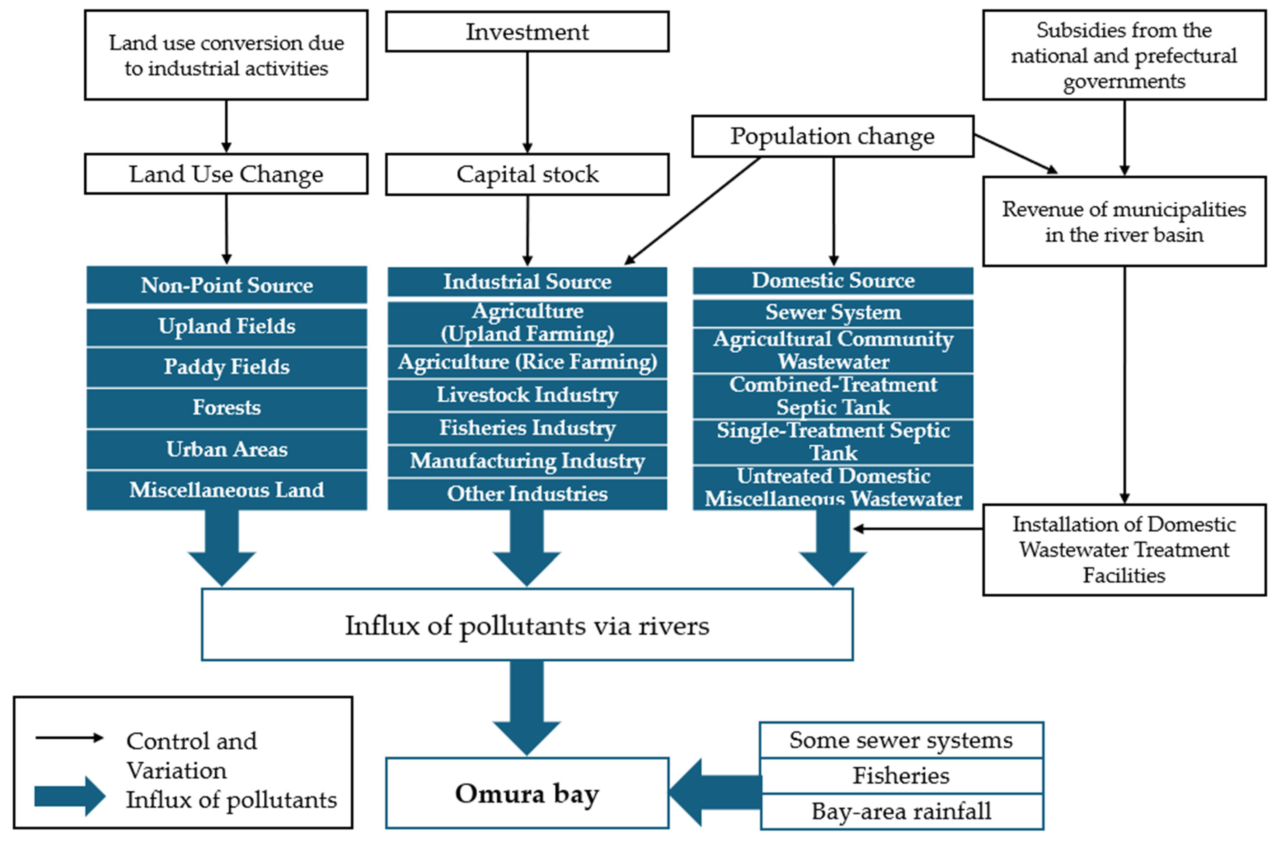
The simulation model was formulated based on the framework developed by Hirose [11] and Mizunoya [17]. This framework is particularly suited for this study as it allows for a detailed analysis of the economic impacts of environmental policies across different industrial sectors. Figure 1 shows the structure of the simulation. The model integrates the socioeconomic activities of the Omura Bay watershed, pollutants flowing into Omura Bay owing to these activities, and policies to reduce pollutants. The pollutants considered were nitrogen, phosphorus, and COD. We assumed that pollutants generated by socioeconomic activities in the watershed flow into Omura Bay through major rivers after undergoing natural purification processes. We also assumed that pollutants from wastewater treatment facilities along the Omura Bay coast, the fishery industry, and rainfall runoff flow directly into the bay.

We classified the pollutants generated from socioeconomic activities within the watershed into three categories: domestic, non-point source, and industrial. Domestic sources were further divided into five types based on wastewater treatment: sewage systems, rural community wastewater treatment, combined-treatment septic tanks, single-treatment septic tanks, and night soil treatment facilities. Sewage systems, rural community wastewater treatment, and combined-treatment septic tanks process both human waste and household wastewater, whereas single-treatment septic tanks and night soil treatment facilities process only human waste. We classified non-point sources into five land-use categories: farmland, rice paddies, forests, urban areas, and miscellaneous land (e.g., fallow land). We classified industrial sources into five categories based on pollution load generation: agriculture (upland and rice farming), livestock, fisheries, manufacturing, and other industries. We assumed that the “other industries” category does not generate pollution loads.

The simulation incorporated policies to reduce pollutants emitted from domestic, non-point, and industrial sources within the watershed. To reduce pollutants from domestic sources, the government introduced policies promoting the development and installation of advanced treatment facilities. These policies increased the use of sewage systems, rural community wastewater treatment, and combined-treatment septic tanks in the population. For non-point sources, policies converting farmland into fallow land and maintaining forest area were implemented. To reduce pollutants from industrial sources, the government implemented policies adjusting production values through subsidies.

2.2. Study Area

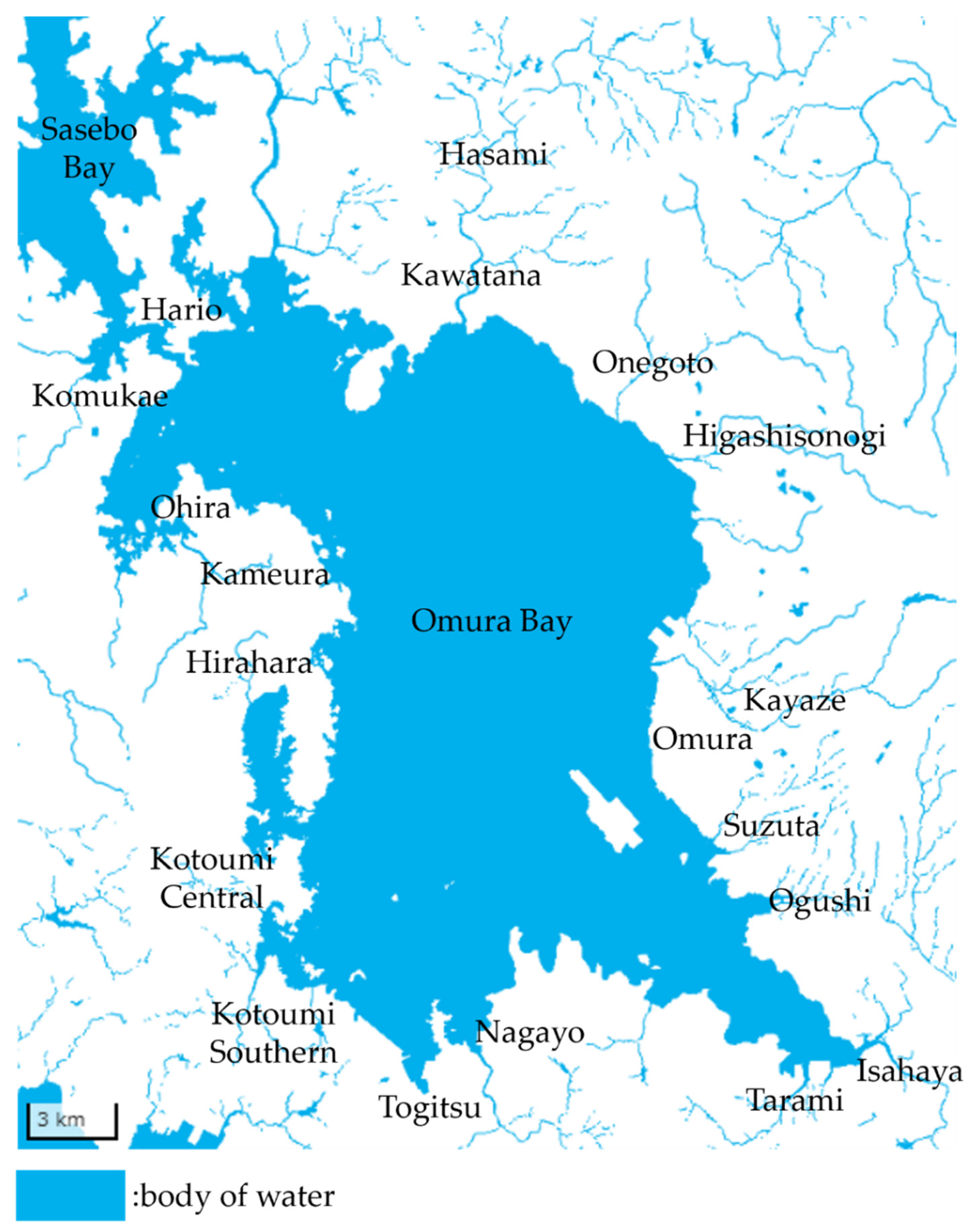
The study area consists of the Omura Bay watershed in Nagasaki Prefecture, with a watershed area of 320 km² and a population of approximately 280,000, accounting for approximately 20% of the total prefectural population. The study area includes five cities (Saikai, Nagasaki, Isahaya, Omura, and Sasebo) and five towns (Togitsu, Nagayo, Higashisonogi, Kawatana, and Hasami). These were further divided into 20 blocks based on wastewater treatment facilities, major rivers, and environmental standard points located downstream in Omura Bay. These are shown in Figure 2. We estimated the area, population, population trends, production value, and capital accumulation for each block from the proportion of the watershed area of the major rivers. Omura Bay is a double-closed bay, connected to the open sea only via the narrow Hario Seto and Haiki Seto straits. This enclosed nature, combined with calm waters, has traditionally supported pearl and oyster farming. However, the watershed has experienced significant human-induced transformations. Shallow coastal areas, such as seagrass beds and tidal flats, have been largely reclaimed, altering the bay’s hydrodynamic characteristics [20]. Population growth and industrial activities have led to pollution loads that surpass the bay’s natural purification capacity [21], resulting in persistent red tides and hypoxic water masses. In response, the Nagasaki Prefectural Government initiated the Omura Bay Environmental Conservation and Revitalization Action Plan in 2003 [22], focusing on improving wastewater treatment coverage. Despite these efforts, water quality standards were frequently not met, leading to the fourth phase of the plan in 2019 [23].

2.3. Model Details

2.3.1. Key Assumptions and Their Validity

This model was constructed based on several key assumptions. We present the rationale for these assumptions and their potential impact on the results. The parameters shown in the Appendix A were calculated using Nagasaki Prefecture’s Input–Output Tables (2015) [24], the Statistical Yearbook 2015 [25], and the Cabinet Office’s data on private enterprise capital stock (2015) [26]. Some data was also directly obtained from local governments in the target area.

Method for Calculating the Pollutant Load: Pollutant loads from various sources were calculated using the unit load method. This is a standard technique used in Japan’s environmental planning, recommended by government agencies such as the Ministry of the Environment [27]. The total load is estimated by multiplying the activity levels by emission factors (pollutant load per unit of activity). The specific values for these factors were derived from established national and local guidelines and are detailed in

Table A2. Pollutant emission coefficients.

Item	T-N	T-P	COD	Unit
E1	1.167	0.037	0.849	kg/people × year	Sewer System
E2	1.062	0.114	0.573	kg/people × year	Agricultural Community Wastewater
E3	2.19	0.214	2.139	kg/people × year	Combined-Treatment Septic Tank
E4	2.792	0.239	1.291	kg/people × year	Single-Treatment Septic Tank
E5	0.931	0.131	5.606	kg/people × year	Untreated Domestic Miscellaneous Wastewater
G1	7.3	0.31	13.57	kg/ha × year	Upland Fields
G2	7.3	0.31	13.57	kg/ha × year	Paddy Fields
G3	5.69	0.197	13.98	kg/ha × year	Forests
G4	8.76	0.657	54.47	kg/ha × year	Urban Areas
G5	7.3	0.31	13.57	kg/ha × year	Miscellaneous Land
P11	2.29	0.029	0.51	kg/million JPY × year	Agriculture (Upland Farming)
P12	1.02	0.026	7.8	kg/million JPY × year	Agriculture (Rice Farming)
P2	13.39	0.337	28.09	kg/million JPY × year	Livestock Industry
P3	101.48	22.425	254.28	kg/million JPY × year	Fishery industry
P4	0.07	0.008	0.12	kg/million JPY × year	Manufacturing Industry
P5	0	0	0	kg/million JPY × year	Other Industries
φ	1124.20	47.45	2091.45	kg/km2	Bay surface area 321 km2: Ll

Source: Hirose [16], Nagasaki Prefecture Government [26], Kunimatsu et al. [29].

in the Appendix A. The emission factors used in this study were derived from values established in the Nagasaki Prefecture environment white book [28], and national environmental guidelines [27]. While this method provides robust, scientifically grounded estimates based on available statistics, it assumes uniform emission patterns within each category and cannot capture detailed location-specific variations.

Linear Relationships: This model employs linear programming, assuming linear relationships between variables (e.g., production volume and capital, investment and pollutant reduction). This simplification is key to the input–output analysis framework, which enables efficient optimization and clear interpretation of economic trade-offs [29]. The nonlinearities existing in real-world environmental and economic systems featuring complex nonlinear relationships—as shown in research by Amazing et al. [30], who applied machine learning models in environmental policy analysis—are acknowledged. However, linearity remains a common and widely accepted assumption in regional-scale economic–environmental modeling for analyzing first-order policy impacts; for example, see Yokosawa et al. [31], Hirose et al. [11], and others.

Base Year: The base year for this model is 2015. This is because of the latest version of the Nagasaki Prefecture Input–output Table [24], which forms the core of the simulation model in this paper. To maintain consistency with this, the data used in this model is from 2015. We recognize that using a single year as the base year carries the risk that the economic conditions specific to that year may influence future projections, potentially limiting the generality and universality of the results. However, the primary objective of this study is not to precisely predict the absolute value of future GRP, but rather to compare and evaluate the relative impacts on the regional economy of different environmental policy scenarios—such as total pollutant load reduction and management tailored to regional characteristics—starting from the 2015 socioeconomic structure. Therefore, this approach avoids unrealistic, abrupt economic fluctuations and simulates the gradual impacts associated with policy implementation. As such, the future GRP and countermeasure costs presented in this paper are reasonable indicators for comparing the relative merits of policies and the magnitude of their economic impacts, rather than as absolute forecast values.

Pollutant Transport: This model assumes that a fixed proportion of pollutants generated within the watershed reaches Omura Bay, determined by the river transport coefficient (κj) representing natural purification. Under this assumption, κj was calculated based on river distances following Kunimatsu et al. [32]. This simplifies complex hydrological processes, and is a major simplification used in many existing studies. The river transport coefficients (κ) for each of the watershed area (j) are provided in

Table A1. Area and flow rate.

		i	j	Flow Rate κj
City Name	Area Name	Code		T-N	T-P	COD	Destination	Channel Extension (km)
Saikai	Komukae	1	1	1.00	1.00	1.00	Omura Bay	0.00
	Ogushi		2	1.00	1.00	1.00	Omura Bay	0.00
	Kameura		3	1.00	1.00	1.00	Omura Bay	0.00
	Hirahara		4	0.69	0.62	0.86	Daimyouji Liver	3.88
Nagasaki	Ohira	2	5	1.00	1.00	1.00	Omura Bay	0.00
	Kotoumi-Central		6	1.00	1.00	1.00	Omura Bay	0.00
	Kotoumi-Southern		7	0.86	0.82	0.94	Muramatsu Liver	1.55
Togitsu	Togitsu	3	8	0.72	0.65	0.87	Togitsu Liver	3.50
Nagayo	Nagayo	4	9	1.00	1.00	1.00	Omura Bay	0.00
Isahaya	Isahaya	5	10	0.42	0.32	0.69	Higashiokawa Liver	9.11
	Tarami		11	0.84	0.80	0.93	Ikiriki Liver	1.83
Omura	Suzuta	6	12	0.58	0.49	0.79	Suzuta Liver	5.77
	Omura		13	1.00	1.00	1.00	Omura Bay	0.00
	Kayaze		14	0.22	0.14	0.53	Korigawa Liver	15.94
Higashi sonogi	Nakao	7	15	0.79	0.73	0.90	Higashisonogi Liver	2.51
	Higashisonogi		16	1.00	1.00	1.00	Omura Bay	0.00
	Onegoto		17	1.00	1.00	1.00	Omura Bay	0.00
Kawatana	Kawatana	8	18	1.00	1.00	1.00	Omura Bay	0.00
Hasami	Hasami	9	19	0.16	0.09	0.46	Kawatana Liver	19.35
Sasebo	Hario	10	20	1.00	1.00	1.00	Omura bay	0.00

Source: Nagasaki Prefecture Government [26], Kunimatsu et al. [29].

.

2.3.2. Pollutant Load Inflow into Omura Bay

Pollutants discharged from the watershed flow into Omura Bay through major rivers. Pollutants from the fishery industry, effluent from wastewater treatment plants along the Omura Bay coast, and direct rainfall on the bay surface also contribute to this direct inflow. Thus, we modeled the pollutant load inflow amount as follows:

$$Q\left(t\right)=\sum _j{a}_j\left(t\right)+Q^F\left(t\right)+\sum _k{Q}_k^S\left(t\right)+Q^r$$

(1)

• $Q\left(t\right)$: Total pollutant load inflow into Omura Bay (kg).
• $a_j\left(t\right)$: Pollutant load inflow from rivers (kg).
• $Q^F\left(t\right)$: Pollutant load from the fishery industry (kg).
• $Q_k^S\left(t\right)$: Pollutant load from wastewater treatment plant effluent (kg).
• $Q^r$: Pollutant load from rainfall over the bay (kg).

The components of the pollutant load inflow are defined as follows. The riverine pollutant load is expressed as:

$$a_j\left(t\right)={\kappa }_j{\gamma }_j\left(t\right)$$

(2)

• ${\kappa }_j$: River transport coefficient representing natural purification capacity.
• ${\gamma }_j$: Pollutant load inflow into rivers from socioeconomic activities (kg).

Regarding pollutant load from socioeconomic activities, we considered the following:

$${\gamma }_j\left(t\right)=E{Z}_j\left(t\right)+G{L}_j\left(t\right)+P{X}_j\left(t\right)$$

(3)

• $E$: Pollutant emission coefficient for domestic sources (row vector).
• $Z_j(t)$: Population by wastewater treatment type (column vector, people).
• $G$: Pollutant emission coefficient for non-point sources (row vector).
• $L_j(t)$: Land Use Area (column vector, ha).
• $P$: Pollutant emission coefficient for industrial sources (row vector).
• $X_j(t)$: Production output by industry (column vector, JPY).

The pollutant load from the fishery industry is assumed to be proportional to the industry’s production value.

$$Q^F\left(t\right)=P^3{x}^3\left(t\right)$$

(4)

where P³ is the pollutant emission coefficient for the fishery industry (row vector) and x³ is the production output of the fishery industry (column vector, JPY).

Wastewater is treated before being discharged into rivers and, eventually, into Omura Bay. However, facilities located along the bay discharge waste directly into the bay. We modeled the pollutant load from wastewater treatment plants as follows:

$$Q_k^S\left(t\right)=E_k^l\sum z_i^l\left(t\right)$$

(5)

The pollutant load from direct rainfall into Omura Bay is calculated based on the bay’s surface area:

$$Q^r=\varphi L_l$$

• $\varphi$: Rainfall pollutant load coefficient.
• $L_l$: Bay surface area (ha).

2.3.3. Domestic Sources

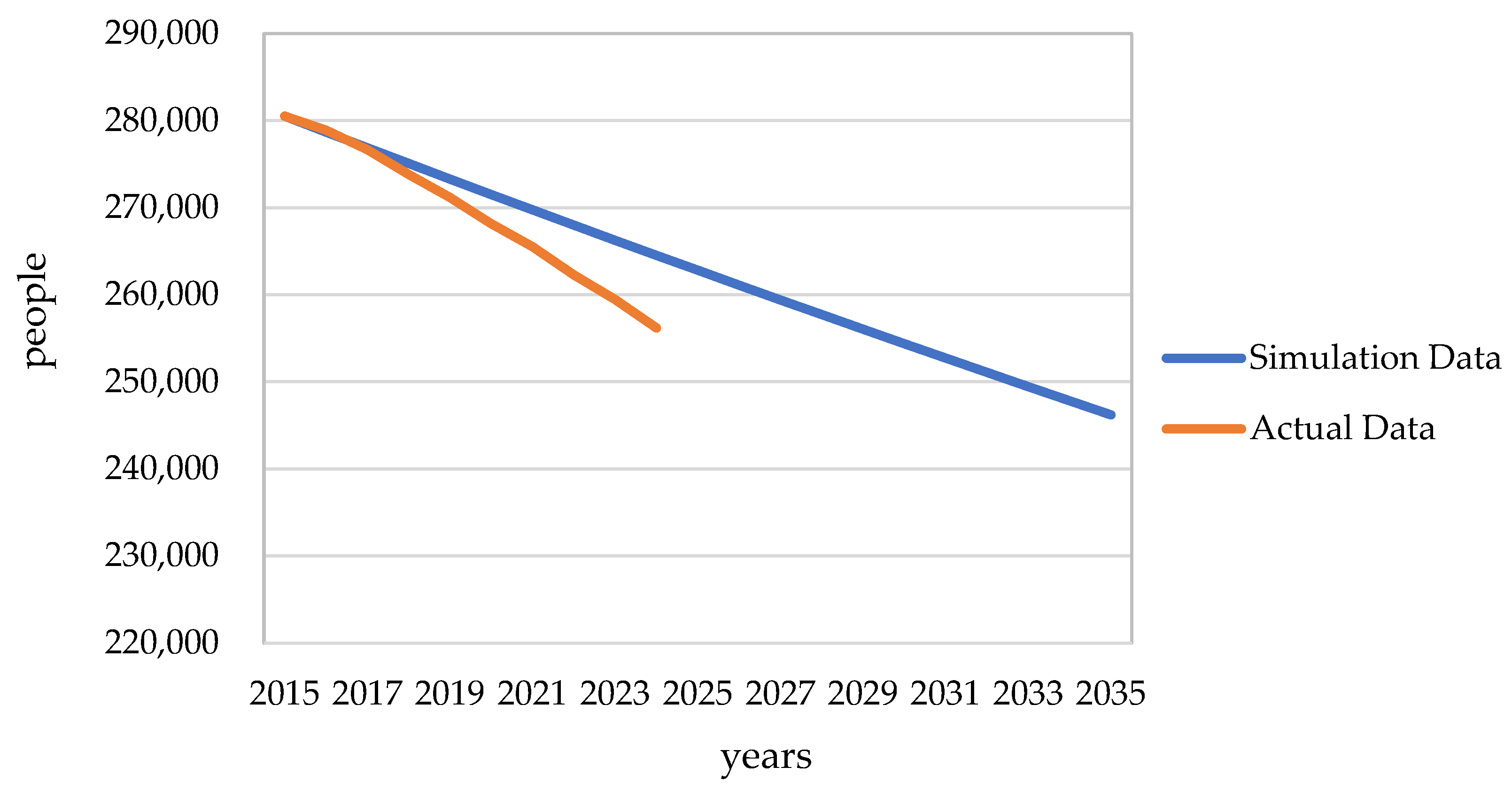
The rate of population change for each municipality in the watershed is assumed to be constant:

$$z_i\left(t+1\right)=z_i\left(t\right)+\Delta z_i$$

(6)

• $\mathsf{\Delta }{z}_i$: Population change

Regarding municipal fiscal revenue, we set the fiscal scale of a municipality as being proportional to its population:

$$R_i\left(t\right)={\rho }_i{Z}_i\left(t\right)$$

(7)

• $R_i\left(t\right)$: Fiscal scale (JPY).
• ${\rho }_i$: Fiscal scale per resident.

The model includes the population served by various domestic wastewater treatment facilities. It is assumed that the total population served by these facilities equals the total municipal population.

$$z_i\left(t\right)=z_i^1\left(t\right)+z_i^2\left(t\right)+z_i^3\left(t\right)+z_i^4\left(t\right)+z_i^5\left(t\right)$$

(8)

• Population using sewer systems (people).
• Population using rural community sewage treatment (people).
• Population using combined treatment septic tanks (people).
• Population using single treatment septic tanks (people).
• Population using night soil treatment facilities (people).

The increase in the population served by sewer systems and rural community sewage treatment is determined by municipal investments in these facilities:

$$\Delta z_i^h\left(t\right)\le {\Gamma }_i^h{i}_j^h\left(t\right)$$

(9)

• $i_j^h(t)$: Investment in facility construction.
• ${\Gamma }_i^h$: Parameter representing facility expansion efficiency.
• h = 1, Sewer systems; h = 2, Rural community sewage treatment.

The development of sewer systems and rural community sewage treatment is funded through municipal bonds and general account budget transfers. Maintenance is financed through usage fees, with any shortfalls covered by general account transfers. In our model, the cumulative project cost for a municipality must not exceed the total project cost:

$$k_i^h\left(t+1\right)=k_i^h\left(t\right)+i_i^h\left(t\right)\le T{B}_i^h$$

(10)

• $k_i^h\left(t\right)$: Cumulative project cost (JPY).
• $T{B}_i^h$: Total project cost (JPY).

Construction investment is determined by the municipality’s financial contributions and corresponding national subsidies.

$$i_i^h\left(t\right)=\left({\displaystyle \frac{1}{1-M_i^h}}\right)c{c}_i^h\left(t\right)$$

(11)

• $M_i^h$: National subsidy ratio for construction.
• $c{c}_i^h(t)$: Municipality’s construction burden (JPY).

$$d{b}_i^h\left(t\right)\le {\epsilon }_i^{h}R\left(t\right)$$

(12)

• ${\epsilon }_i^h$: Bond issuance ratio

Changes in the population using combined-treatment septic tanks are also modeled. This population increases through installation subsidies but decreases as sewer systems and rural community sewage treatment expand:

$$z_i^3\left(t+1\right)=z_i^3\left(t\right)+\Delta z_i^3-{\tau }_i\left(\Delta z_i^1\left(t\right)+\Delta z_i^2\left(t\right)\right)$$

(13)

• ${\tau }_i$: Transition rate from combined-treatment septic tanks to sewer systems and rural community sewage treatment.

The subsidies for installing combined-treatment septic tanks are provided by national and prefectural governments, along with the general account budgets of municipalities. Our model accounts for this relation as follows:

$$\delta \Delta z_i^3\left(t\right)=\left({\displaystyle \frac{1}{1-M^3}}\right)b_i^3\left(t\right)$$

(14)

• δ: Installation cost per person for combined-treatment septic tanks (JPY).
• $M^3$: Subsidy ratio from national and prefectural governments.
• $b_i^3$: Municipality’s subsidy contribution (JPY).

The municipal expenditure for sewerage system development, rural community wastewater treatment, and subsidies for combined-treatment septic tank installations is determined by the financial capacity of each municipality. In our model, the constraint is expressed as follows:

$$b_i^1\left(t\right)+b_i^2\left(t\right)+b_i^3\left(t\right)+g_i^1+b_i^2\le \omega R_i\left(t\right)+s_i^1\left(t\right)$$

(15)

• $\omega$: Ratio of financial resources allocated for domestic wastewater treatment.
• $s_i^1(t)$: Subsidies for domestic wastewater treatment.

This equation ensures that the total spending on wastewater management does not exceed the financial resources available to the municipality. Moreover, our model considered the transition of the population using different sanitation systems and night soil treatment facility, represented in Equations (15) and (16), respectively:

$$z_i^4\left(t+1\right)=z_i^4\left(t\right)+{\pi }_i\left(\Delta z_i\left(t\right)-\left(1-{\tau }_i\right)\left(\Delta z_i^1\left(t\right)+\Delta z_i^2\left(t\right)\right)-\Delta z_i^3\left(t\right)\right)$$

(16)

• ${\pi }_i$: Parameter controlling transition to other sanitation systems.

$$z_i^5\left(t+1\right)=z_i^5\left(t\right)+\left(1-{\pi }_i\right)\left(\Delta z_i\left(t\right)-\left(1-{\tau }_i\right)\left(\Delta z_i^1\left(t\right)+\Delta z_i^2\left(t\right)\right)-\Delta z_i^3\left(t\right)\right)$$

(17)

2.3.4. Non-Point Sources

The total land use area equals the total area of each municipality within the Omura Bay watershed. Our model accounted for land use as follows:

$$\overline{L_J}=\sum _{k=1}^5{L}_j^k(t)$$

(18)

• $L_j^k(t)$: Area of land use type k (ha)

Our model also accounted for land use changes owing to conversions between different land use types.

$$L_j^k\left(t+1\right)=L_j^k\left(t\right)+\sum _{k\ne l}{L}_j^{lk}\left(t\right)-\sum _{l\ne k}{L}_j^{kl}\left(t\right)$$

(19)

• $L_j^{lk,kl}\left(t\right)$: Conversion from land use l to k (or vice versa).

In this study, we noted that direct conversion from forests and farmland to urban areas was restricted. Conversion to urban areas was only allowed from mixed-use land. Forest areas remained unchanged, and farmland could only be converted into mixed-use land.

Our study also accounted for the policy introduced to provide subsidies for fallowing farmland.

$$L_j^{k5}\left(t\right)\ge {\lambda }^k{s}_j^m\left(t\right)$$

(20)

• ${\lambda }^k$: Parameter. k = 1, 2, m = 2, 3.

The change in urban and mixed-use land area is considered as follows. The increase in urban area is proportional to population growth and investments in manufacturing and other industries.

$$L_j^{54}\left(t\right)\ge \xi \Delta z_j\left(t\right)+{\varphi }^4\Delta i_j^{4P}\left(t\right)+{\varphi }^5\Delta i_j^{5P}\left(t\right)$$

(21)

• $\xi$: Residential land demand function.
• ${\varphi }^{\mathrm{4,5}}$: industrial land demand function.
• $\mathsf{\Delta }{i}_j^{4P,5P}(t)$: Expansion in investment in manufacturing and other industries.

Finally, our model reflected the changes in mixed-use land area owing to conversion from farmland and conversion to urban land.

$$L_j^5\left(t+1\right)=L_j^5\left(t\right)+L_j^{15}\left(t\right)+L_j^{25}\left(t\right){-L}_j^{54}\left(t\right)$$

(22)

2.3.5. Industrial Sources

The level of production depends on capital accumulation. As agriculture heavily relies on farmland, farmland is also considered a form of capital accumulation. We accounted for production constraints as follows:

$$x_j^n\left(t\right)\le {\alpha }^n{k}_j^{nP}\left(t\right)$$

(23)

• ${\alpha }^n$: Production constraint coefficient.
• n = 11, upland farming; n = 12, rice farming; n = 2, livestock industry.
• n = 3, fisheries; n = 4, manufacturing industry; n = 5, other industries.

The dynamics of capital accumulation are defined as follows. Capital decreases due to depreciation and increases through investment. The model incorporates a policy to regulate production and reduce pollution loads by providing subsidies that decrease capital. In agriculture, capital also decreases as farmland is reduced.

For agriculture,

$$k_j^{nP}\left(t\right)=k_j^{nP}\left(t-1\right)-d^n{x}_j^n\left(t-1\right)+i_j^{nP}\left(t\right)-{\theta }^n{L}_j^{n5}\left(t\right)-f^n{s}_j^m\left(t\right)$$

(24)

For industries other than agriculture,

$$k_j^{nP}\left(t\right)=k_j^{nP}\left(t-1\right)-d^n{x}_j^n\left(t-1\right)+i_j^{nP}\left(t\right)-f^n{s}_j^m\left(t\right)$$

(25)

• $k_j^{nP}\left(t\right)$: Capital accumulation of each industry (JPY).
• $i_j^{nP}\left(t\right)$: Investment amount of each industry (JPY).
• $d^n$: Depreciation rate for each industry (JPY).
• $s_j^m(t)$: Subsidy for each industry (JPY).
• ${\theta }^n,f^n$: Parameters.

$$L_j^{115}\left(t\right)\to L_j^{15}\left(t\right),\ast L_j^{125}\left(t\right)\to L_j^{25}\left(t\right)$$

(26)

2.3.6. Omura Bay Countermeasure Costs

Nagasaki Prefecture allocates a budget for countermeasure costs to reduce the pollution load in Omura Bay. We accounted for Omura Bay countermeasure costs as follows:

$$y(t)=\sum _i{S}_i^l+\sum _j\sum _m{S}_j^m(t)$$

(27)

• $\mathrm{y}\left(\mathrm{t}\right)$: Omura Bay countermeasure costs (JPY).

2.3.7. Economic Indicators

In our model, the production value of each industry follows the following flow conditions in the product market.

$$x\left(t\right)\ge Ax\left(t\right)+C\left(t\right)+i^P\left(t\right)+B^S\left(i^1\left(t\right)+i^2\left(t\right)\right)+B^C\left(\delta \Delta Z^3\left(t\right)\right)+e(t)$$

(28)

$$x(t)=\sum _j{x}_j(t)$$

• Sector-wise production value column vector for the entire watershed

$$i^p(t)=\sum _j{i}_j^P(t)$$

• Production investment column vector for the entire watershed

$$i^h(t)=\sum _i{i}_i^h(t)$$

• Total investment in sewage and agricultural village drainage system construction (JPY)
• A: Input–output coefficient matrix.
• C(t): Consumption column vector.
• $B^S,B^C$: Sector-wise production inducement coefficient column vectors for sewage system improvements, agricultural village drainage, and combined-treatment septic tank installation.
• e(t): Net export column vector.

Consumption is constrained by the total population within the watershed. We accounted for consumption constraints as follows:

$$C\left(t\right)=H\sum _i{z}_i\left(t\right)$$

(29)

• H: Sector-wise consumption coefficient column vector.

We accounted for net export constraints as follows:

$$e_{min}\le e\le e_{max}$$

(30)

• $e_{min},e_{max}$; Lower and upper limits of net export.

Regarding GRP, we used the GRP as the economic indicator for municipalities, defined as the sum of the value added by each industry.

$$GRP\left(t\right)=vx\left(t\right)$$

(31)

• v: Value-added rate row vector for each industry.

2.3.8. Objective Function and Limiting Condition

We set target values for the pollution load flowing into Omura Bay to maximize the GRP of the municipalities in the Omura Bay watershed while satisfying this constraint at time T. The objective of this research is to find the optimal policy that minimizes socioeconomic costs (equivalent to maximizing achievable GRP) while ensuring that environmental standards are met as a constraint. The following equation represents the objective function and constraints. The objective function is to maximize GRP, while the constraints involve controlling the inflow of pollutants. This approach is valid as a constrained optimization problem, as it seeks the option with the least economic impact within the absolute constraint of environmental standards. This allows for a quantitative evaluation of the trade-off between the environment and the economy.

$$MAXGRP\left(T\right)$$

(32)

$$subjecttoQ\left(t\right)\le Q^{\ast }\left(t\right)$$

(33)

• $Q^{\ast }$: Target value for the pollution load flowing into Omura Bay.

2.4. Simulation

We conducted the simulation using LINGO, a mathematical computation software by LINDO SYSTEMS. The baseline was established by calculating the pollutant load emissions and GRP of the watershed based on data from the 62nd Edition of the Nagasaki Prefecture Statistical Yearbook. In addition, the simulation employed a model constructed using the 2015 Nagasaki Prefecture Input–Output Table. We employed two scenarios to modify the constraints on pollutant inflow. Additionally, to prevent abrupt changes in socioeconomic activities within the watershed over a short period, we limited the annual decrease in production value for each industry to a maximum of 10% per year and up to 30% of the 2015 level.

2.4.1. Scenario 1: Reduction in Total Pollutant Load Inflow

Scenario 1 aimed to determine the achievable total reduction in pollutant inflow into Omura Bay without significantly impacting socioeconomic activities in the watershed. As a constraint condition in the simulation, total emission limits were set for three pollutants: COD, total nitrogen, and total phosphorus. We set the regulatory reduction rates at four levels: 0%, 5%, 10%, and 15% of the total pollutant load in Omura Bay in 2015.

2.4.2. Scenario 2: Pollutant Load Management

Scenario 2 aimed to explore the feasibility of introducing an appropriate pollutant load management policy in the Omura Bay watershed, considering the impact of significant water quality improvements on the fishery industry. We set water quality target values for COD, total nitrogen, and total phosphorus (

Table 1. Water quality target values.

Water Quality Target	COD	T-N	T-P
	(mg/L)	(mg/L)	(mg/L)
Environmental standard value (upper limit) in the Omura Bay *1	2.0	0.20	0.020
Environmental standard value (lower limit) in the Seto Inland Sea *2	2.0	0.20	0.020
Water quality target in this study	2.0	0.20	0.020

*1, Nagasaki Prefecture Government [23]; *2, Hyogo Prefecture Environmental Council, Water Environment Subcommittee [8].

). For each of the 20 blocks in the study area, we determined the pollutant inflow target values based on the pollutant with the worst actual water quality relative to the target value in Omura Bay.

Since the environmental measurement data for 2015 was not publicly available, we used the data from 2017 [8], the closest year with published information, to set the target pollutant inflow load values. Therefore, this scenario was conducted using the pollutant inflow load for 2017. The set pollutant load target values are adopted in the model strictly as constraint conditions and do not affect the model’s structure or the simulation dynamics. Additionally, for convenience, the following proportional Equation (34) was assumed to hold, and achieving the pollutant load target value by 2035 was set as a constraint in the simulation.

$${\displaystyle \frac{ActualWaterQuality\left(2017\right)}{WaterQualityTargetValue}}={\displaystyle \frac{PollutantInflowLoad\left(2017\right)}{PollutantInflowLoadTargetValue}}$$

(34)

The water quality target values were set to be optimal for both environmental concerns and the fishery industry. For this study, the target for environmental concerns was defined as the current upper limit of the environmental standard for Omura Bay, set by the Ministry of the Environment. The target for the fishery industry was defined as the lower water quality target limit adopted in the Seto Inland Sea [8], which is the only region in Japan with such a lower limit. As shown in Table 1, these two target values coincided. Therefore, this value was adopted as the water quality target for this research. Based on 2017 levels, the pollutant inflow targets for 2035 were set as follows:

• COD: Increased in five regions, reduced in eight regions, and constant in four regions.
• Total nitrogen (T-N): Reduced in two regions.
• Total phosphorus (T-P): Reduced in one region.

3. Results

3.1. Simulation of the Current Situation

We set the GRP and pollutant discharge loads calculated from 2015 statistical data as the baseline for the simulation (

Table 2. GRP of the Omura Bay watershed.

Industry	Added Value (Million JPY)
Agriculture	9731
Livestock Industry	1723
Fisheries	8004
Manufacturing	77,147
Other Industries	448,162
Total GRP	544,767

Source: Nagasaki Prefecture [24].

and

Table 3. Pollutant load discharge by category in 2015.

Source	Frame	COD	Total Nitrogen	Total Phosphorus
		(kg/year)	(kg/year)	(kg/year)
1. Domestic Sources	Population (people)
Sewer System	231,805.51	196,802.87	270,285.22	8345
Agricultural Community Wastewater	12,227.76	7006.51	12,985.88	1393.96
Combined-Treatment Septic Tank	19,514.83	41,742.23	42,737.49	4176.17
Single-Treatment Septic Tank	2740.99	3538.62	7652.84	820.19
Untreated Domestic Miscellaneous Wastewater	18,328.25	102,748.18	17,063.6	2401
Total (Domestic)	284,040.09	351,838.4	350,725.03	16,971.23
2. Non-Point Sources	Area (ha)
Upland Fields	6131.9	83,209.91	44,762.88	1900.89
Paddy Fields	3889.3	52,777.85	28,391.92	1251.06
Forests	12,183.72	170,328.44	69,325.32	2408.59
Urban Areas	3835.03	208,894.09	359,304.68	2519.41
Miscellaneous Land	2423.21	32,883.01	17,689.46	751.58
Total (Non-point) (Non-Point Source)	29,775.62	548,093.29	193,764.5	8777.58
3. Industrial Sources	Production value (JPY million)
Agriculture (Upland Farming)	8830.65	4503.63	20,222.19	256.09
Agriculture (Rice Farming)	5862.1	45,724.36	5979.34	152.41
Livestock Industry	6216.89	174,632.54	83,244.2	2095.09
Fishery industry	12,382.77	779,087.13	310,924.03	68,707.29
Manufacturing Industry	225,708.05	27,084.97	15,799.56	186.23
Other Industries	741,745.12	0	0	0
Total (Industrial)	1,011,775.3	1,031,263.62	436,169.33	73,017.1
4. Direct Rainfall
	321	671,355.45	360,868.2	15,231.45
Total Pollutant Load Discharge		2,602,319.77	1,341,527.06	113,997.36

). The GRP within the watershed is predominantly composed of the “Other Industries” sector, accounting for 82%, followed by the manufacturing industry at 14%. This indicates that the economy of the Omura Bay watershed is highly influenced by changes in these two sectors. Given our assumption that “Other Industries” generate no pollutant emissions, the impact of pollutant reduction policies on GRP is expected to be most significant in the manufacturing sector.

Focusing on the statistical data and pollutant discharge loads, 7.4% of the population’s pollutant discharge within the watershed remains untreated. Among wastewater treatment facilities, sewage systems are the most prevalent, followed by agricultural community wastewater treatment systems. This suggests that the advancement of high-level wastewater treatment facilities in the Omura Bay watershed is relatively well-developed.

In terms of land use area, forests occupy the largest portion, followed by farmland and rice paddies. Regarding pollutant emissions, production-based sources contribute the most, with the fishery industry accounting for approximately 30% of COD, 23% of total nitrogen, and 60% of total phosphorus. Livestock farming also had a significant share.

For domestic sources of pollution, sewage systems are the largest contributors, responsible for approximately 56% of COD, 77% of total nitrogen, and 49% of total phosphorus. Among the population with untreated discharge, emissions account for around 30% of COD, 7% of total nitrogen, and 18% of total phosphorus. Meanwhile, non-point source pollution is relatively minor, but COD emissions originating from urban areas are the second highest after the fishery industry.

3.2. Scenario 1: Reduction in Pollutant Load Without Impacting Socioeconomic Activities

3.2.1. Modification of Simulation Cases

In this simulation, we obtained feasible solutions for reduction rates of 0%, 5%, and 10%. However, no feasible solution was found for the 15% reduction case. To determine the maximum achievable reduction level, we conducted additional simulations. We set the reduction constraints to 11%, 12%, 13%, and 14%. As a result, we found feasible solutions for the 11% and 12% cases. To accurately identify the boundary of this feasible constraint, a feasible region analysis was conducted. We ran the full linear programming optimization model iteratively, increasing the reduction constraint from 12.1% to 15% in 0.1% increments. The LP model returned feasible solutions for reductions from 12.1% to 12.7%. However, for constraints of 12.8% or higher, the model correctly identified them as infeasible. This iterative process is based on Linear Programming, and LP mathematically guarantees an optimal solution (the maximum GRP) for any given set of feasible constraints. The process described here is a standard approach used only to pinpoint the absolute limit of the feasible region’s boundary, not to search for the optimal solution itself.

3.2.2. Data Validation and Changes in the Objective Function

Figure 3 compares the changes in the optimal objective function (GRP) calculated by the LP model with the actual GRP trends for each feasible reduction constraint identified in Section 3.2.1. The results show that reductions from 0% to 12.3% do not negatively impact GRP. However, for reductions of 12.4% or more, GRP began to decline as the reduction rate increased. Specifically, at a 12.3% reduction, GRP decreased by approximately 0.2% compared with the 0% reduction case. By contrast, at a 12.7% reduction, GRP decreased by approximately 16.3%. These findings suggest that the maximum pollutant reduction achievable by 2035 (compared with 2015 levels) in the Omura Bay watershed, without negatively impacting socioeconomic activities, is 12.3%. Furthermore, a comparison of these results with actual data trends shows that they follow roughly the same behavior until 2019. However, the actual data shows a declining trend after 2019, and the divergence from the simulation is significant. This is thought to be because the socioeconomic structure changed from the base year due to the 2019 consumption tax increase and the COVID-19 pandemic from 2020 onwards. Additionally, Figure 4 compares actual population trends with simulated population trends. This shows that while the trends largely matched until 2018, the decline has been more pronounced thereafter. It is inferred that the aforementioned stagnation in socioeconomic activities impacted population dynamics. Based on the above, the simulation conducted in this study reproduces the real world to some extent. However, it is important to note that it does not reflect events that were unforeseeable at the time of the base year.

3.2.3. Budget Allocation for Countermeasures in Omura Bay

Figure 5 shows the total cumulative countermeasure costs over 20 years and allocation ratio of cumulative countermeasure costs for each policy in three scenarios—maintaining the status quo in 2015 (0% reduction), maximizing reduction without affecting socio-economic activities (12.3% reduction), and maximizing reduction overall (12.7% reduction). The countermeasure cost was highest in the case of maximum reduction, amounting to JPY 4.5 trillion. Additionally, the countermeasure cost for maintaining the status quo exceeded that of the maximum reduction without socioeconomic impact by JPY 109 billion.

Regarding the countermeasure costs by policy, in the case of maintaining the status quo, the cost for the policy of developing domestic wastewater treatment facilities was JPY 275 billion, accounting for 62.0% of the total, followed by the fallow farmland policy at JPY 78 billion (17.5%), the livestock production adjustment policy at JPY 48 billion (10.9%), and the fishery production adjustment policy at JPY 42 billion (9.4%). As the reduction rate increased, the proportion of costs allocated to the fallow farmland, paddy field fallow, and rice production adjustment policies increased, whereas the costs allocated to the policies for domestic wastewater treatment facility development and fisheries production adjustment decreased.

For reductions exceeding 12.3%, the manufacturing production adjustment policy became necessary. As the reduction rate increased, the cost of the manufacturing production adjustment countermeasure also increased. In the 12.7% reduction case, this cost reached JPY 4.165 trillion. This amount alone accounted for 92.8% of the total countermeasure cost.

3.3. Scenario 2: Watershed Management Tailored to Regional Characteristics

In Scenario 2, we successfully achieved the target values set for each region.

Table 4. Regions with increased COD and pollutant emissions.

Region	COD (mg/L)		Total Nitrogen (mg/L)		Total Phosphorus (mg/L)
	2017	2035	2017	2035	2017	2035
Komukae	12.29	16.39	8.49	9.06	0.36	0.41
Ogushi	7.92	10.56	5.74	8.16	0.18	0.48
Kameura	3.43	4.29	2.31	2.45	0.09	0.11
Hirahara	25.52	31.9	17.63	18.74	0.56	0.63
Togitsu	38.65	40.69	39.71	44.42	2.12	2.46

,

Table 5. Regions with decreased COD and pollutant emissions.

Region	COD (mg/L)		Total Nitrogen (mg/L)		Total Phosphorus (mg/L)
	2017	2035	2017	2035	2017	2035
Ohira	11.71	11.16	11.97	11.45	0.38	1.01
Kotoumi Central	4.78	4.56	2.63	2.67	0.14	0.14
Kotoumi Southern	43.87	41.78	44.05	42.34	1.37	3.63
Tarami	17.43	16.6	12.37	12.97	0.53	0.54
Suzuta	17.82	15.5	8.39	8.43	0.35	0.34
Omura	124.49	118.56	129.51	118.55	3.9	10.02
Kawatana	51.64	44.91	39.17	37.36	1.34	1.6
Hasami	78.58	68.34	50.18	50.68	1.74	1.96

,

Table 6. Regions with maintained COD levels and pollutant emissions.

Region	COD (mg/L)		Total Nitrogen (mg/L)		Total Phosphorus (mg/L)
	2017	2035	2017	2035	2017	2035
Kayaze	46.94	46.94	25.66	25.54	1.05	1.03
Nakao	23.35	23.35	14.31	15.04	0.44	0.46
Higashisonogi	35.24	35.24	23.51	23.9	0.64	0.78
Onegoto	8.73	8.73	5.47	5.82	0.22	0.24

,

Table 7. Regions with decreased total nitrogen and pollutant emissions.

Region	COD (mg/L)		Total Nitrogen (mg/L)		Total Phosphorus (mg/L)
	2017	2035	2017	2035	2017	2035
Nagayo	75.99	241.11	80.01	48.49	3.15	5.39
Isahaya	74.37	115.47	62.05	42.8	2	2.42

and

Table 8. Regions with decreased total phosphorus and pollutant emissions.

Region	COD (mg/L)		Total Nitrogen (mg/L)		Total Phosphorus (mg/L)
	2017	2035	2017	2035	2017	2035
Hario	23.95	21.07	17.26	17.41	0.78	0.71

present the projected pollutant inflow for each region in 2035 under this scenario. In regions where COD increased, total nitrogen and total phosphorus also showed an increase. Conversely, in regions where COD decreased, the changes in total nitrogen and total phosphorus varied. Notably, total nitrogen increased only in Tarami and Hasami, whereas total phosphorus increased in most regions, including Ohira, Southern Kotonami, Taramizu, Omura, Kawatana, and Hasami. In regions where COD levels were maintained, we observed little to no change in any of the pollutants. In Nagayo and Isahaya, where total nitrogen was reduced, both COD and total phosphorus increased, with a particularly significant rise in COD. Meanwhile, in Hario, where total phosphorus was reduced, COD increased while total nitrogen decreased. These findings indicate that responses to interventions differ across regions, and that these regional variations significantly influence pollutant control outcomes. The results also highlight a strong correlation between changes in COD and total phosphorus levels.

3.4. Regional Emissions

Figure 6, Figure 7 and Figure 8 show the regional cumulative emissions of COD, total nitrogen, and total phosphorus, respectively. The emissions vary according to the socioeconomic conditions, such as population, land use area, and industrial structure, across regions. Additionally, the dominant pollutant differs by region. Emissions are particularly high in Omura and Togitsu; this notable finding can be attributed to the large population in these areas, which leads to increased economic activities and, consequently, higher pollutant emissions. Given these regional variations, implemented measures need to be tailored to the specific characteristics of each area.

4. Discussion

4.1. The Difference in GRP

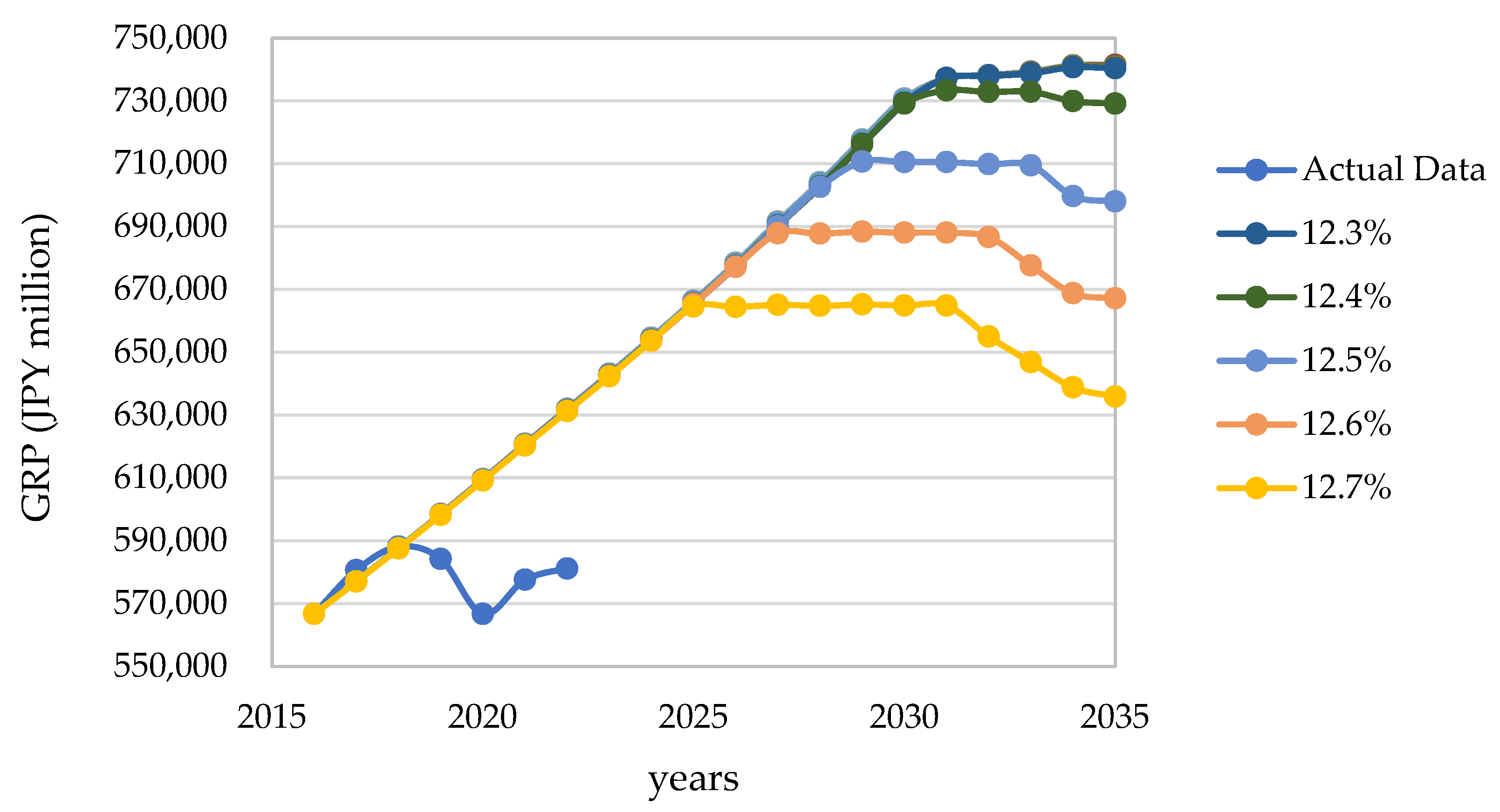
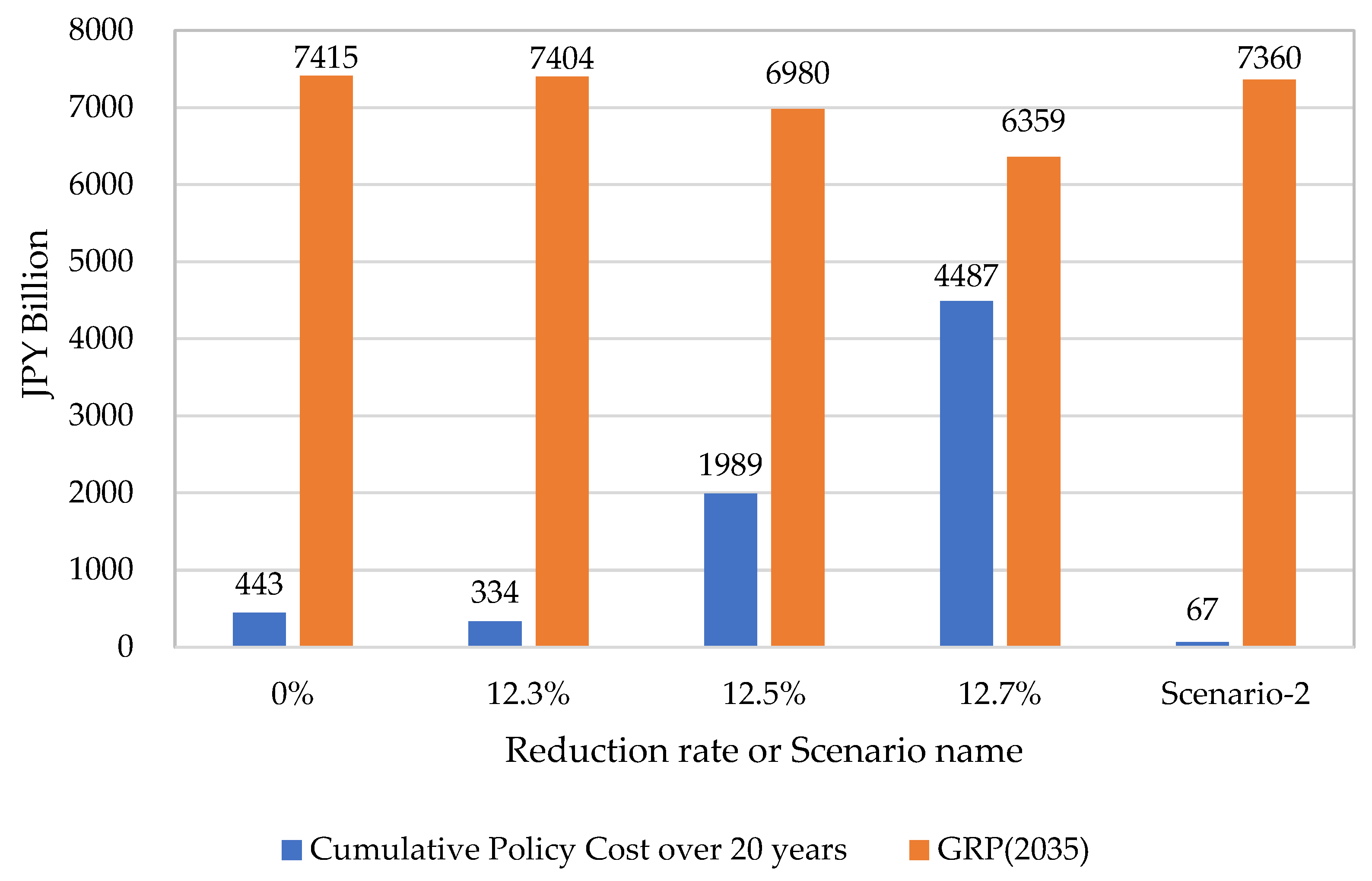
Figure 9 shows the differences in GRP when inflow is managed, the current conditions are maintained, and the total amount is reduced. The final GRP in 2035 under the inflow management scenario was JPY 7.360 trillion. This value is approximately JPY 5.5 billion lower compared with the 0% reduction case, where current conditions were maintained, and approximately JPY 4.5 billion lower compared with the 12.3% reduction case, where the maximum possible reduction was achieved without significantly decreasing GRP. However, this value is also approximately JPY 100 billion higher compared with the 12.7% reduction case, in which maximum reductions are the goal. As the decrease compared to that under the situation maintaining the current conditions was only about 0.8%, the policy of managing inflow had little impact on the GRP.

4.2. Budget Allocation for Countermeasures in Omura Bay

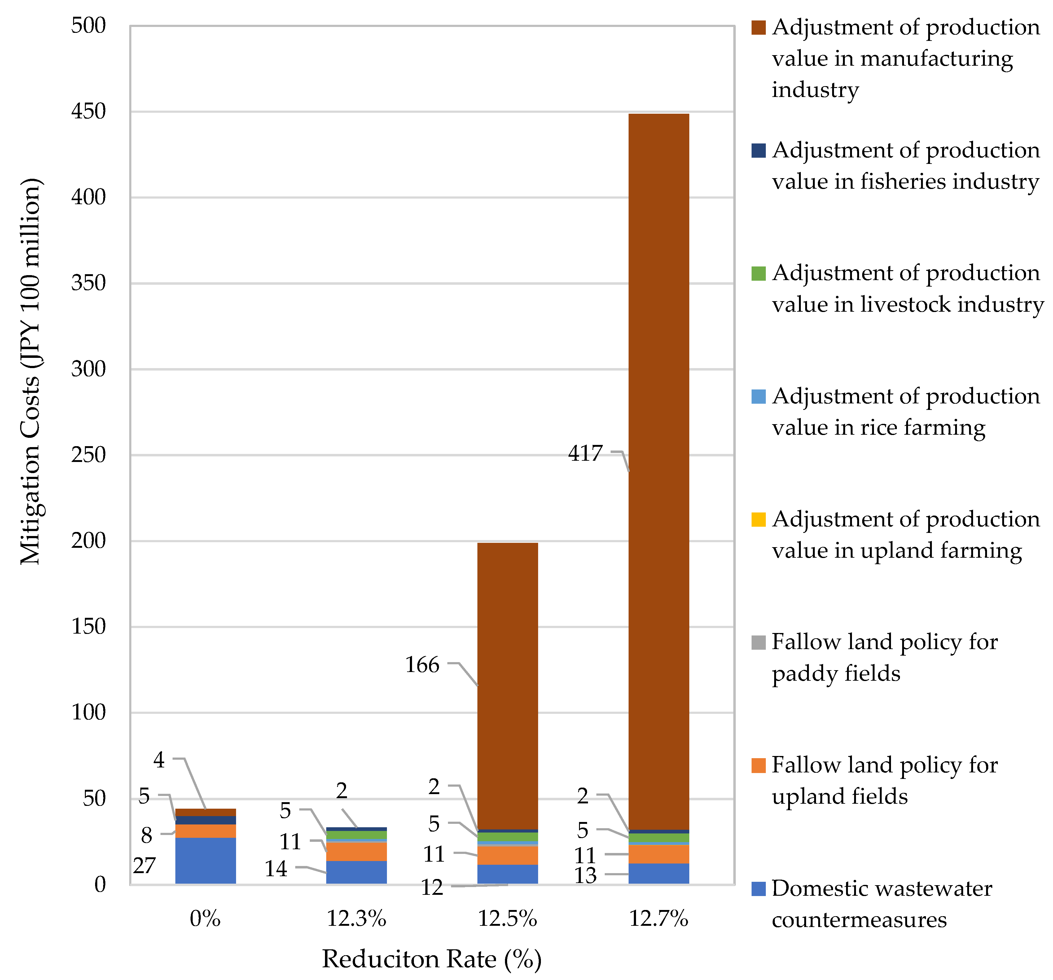
The findings indicate that the domestic wastewater treatment facility development policy is highly cost-effective and can be prioritized owing to its minimal impact on GRP. Additionally, production adjustment policies in the fisheries and livestock industries, which had particularly high emission ratios in 2015, are also highly effective. Furthermore, when the reduction rate exceeds 12.3%, reducing inflow pollution through production adjustments may be prioritized over domestic countermeasures. Although production adjustment policies can lower the GRP, and the manufacturing production adjustment policy significantly increases countermeasure costs, they also yield substantial reductions in pollutant inflows.

Figure 9 shows the countermeasure costs in the cases of 0% reduction in inflow pollutants, 12.3% reduction, and inflow management. The results indicate that the inflow management policy scenario (Scenario 2) can significantly reduce countermeasure costs, making it an effective approach. Meanwhile, GRP is higher in the case of total reduction; therefore, when implementing inflow management policies in practice, the impact on GRP must be minimized as much as possible.

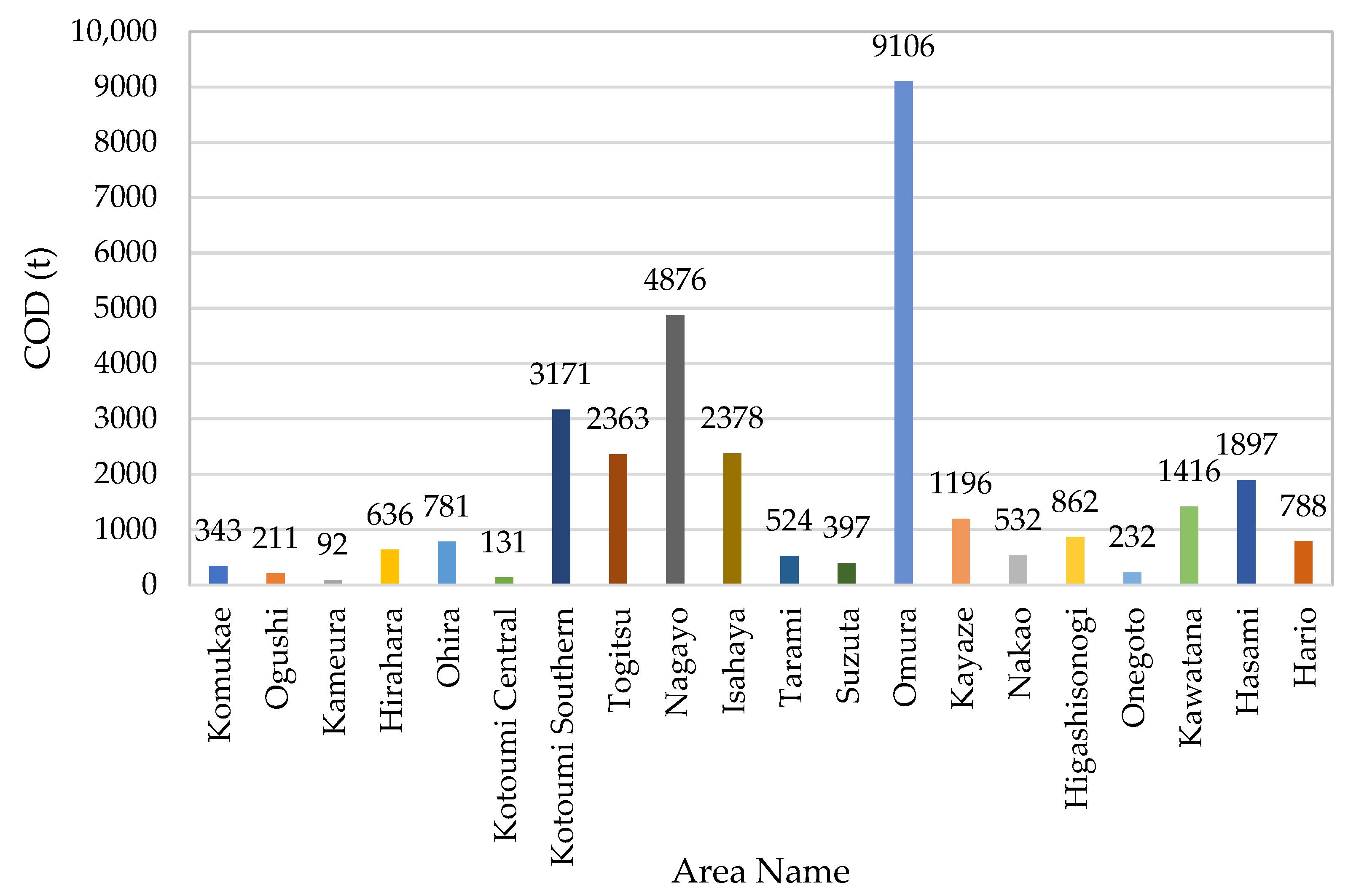
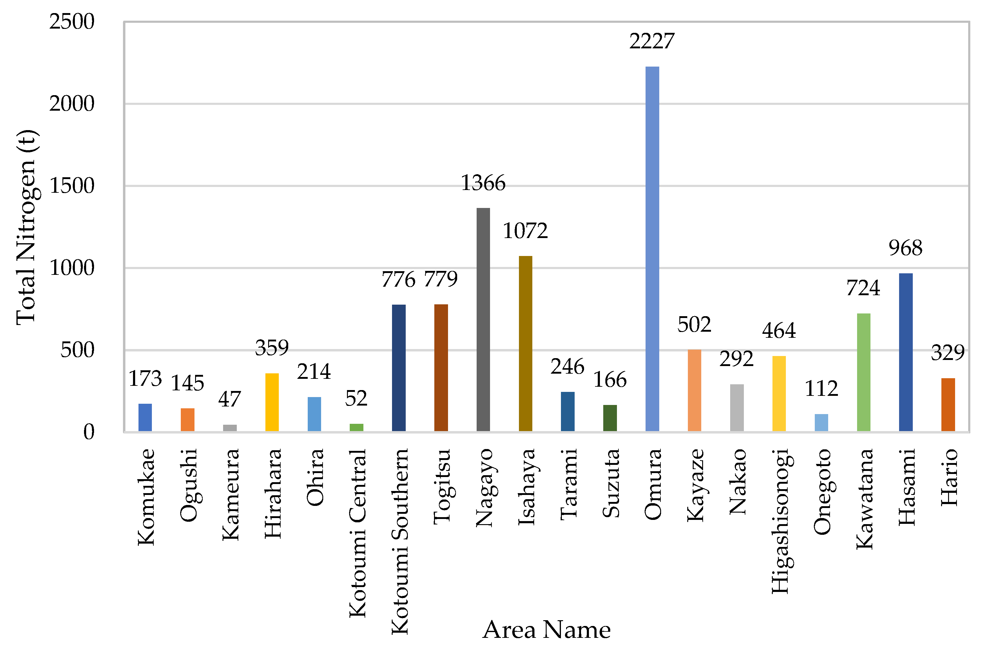
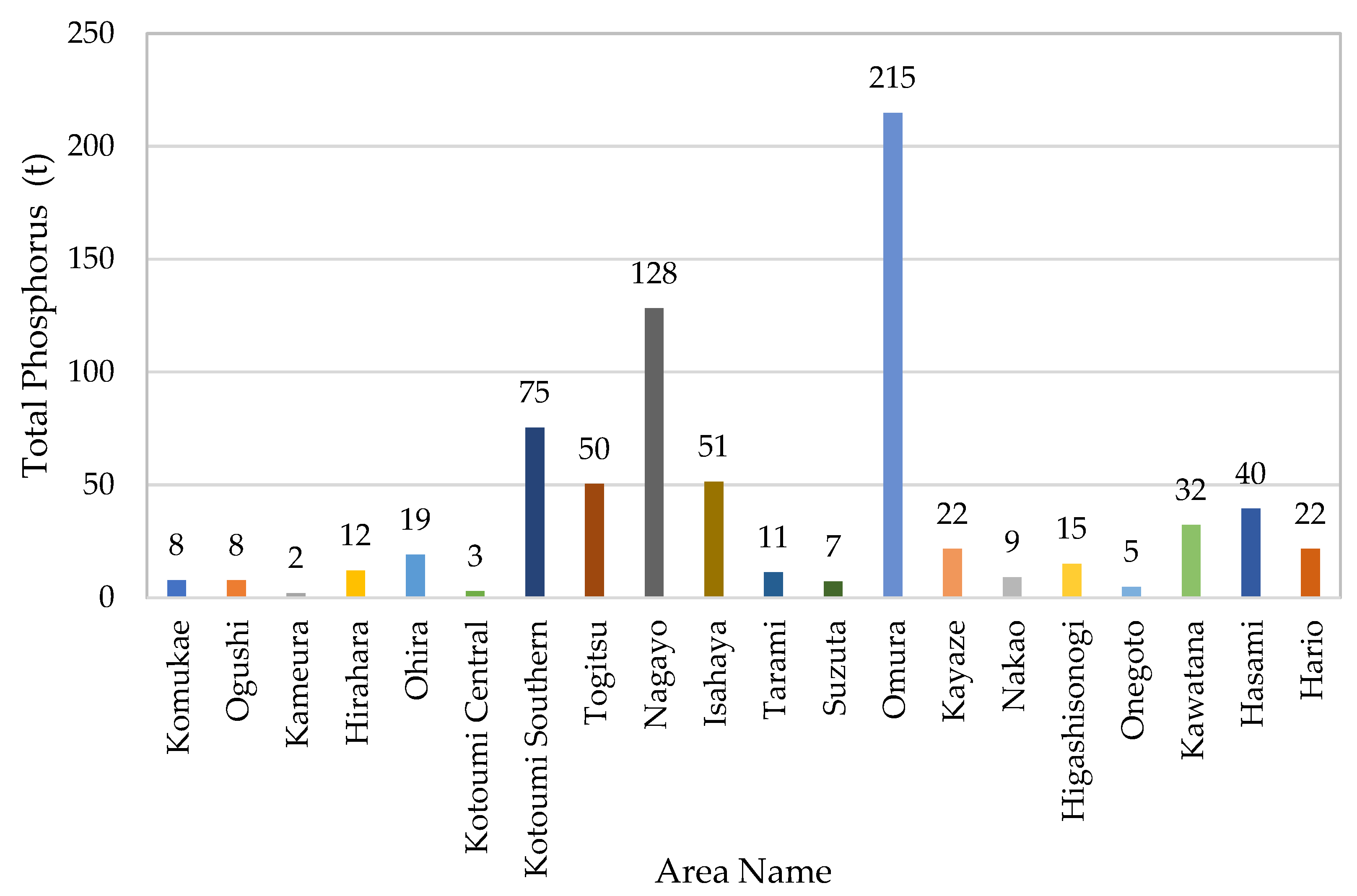
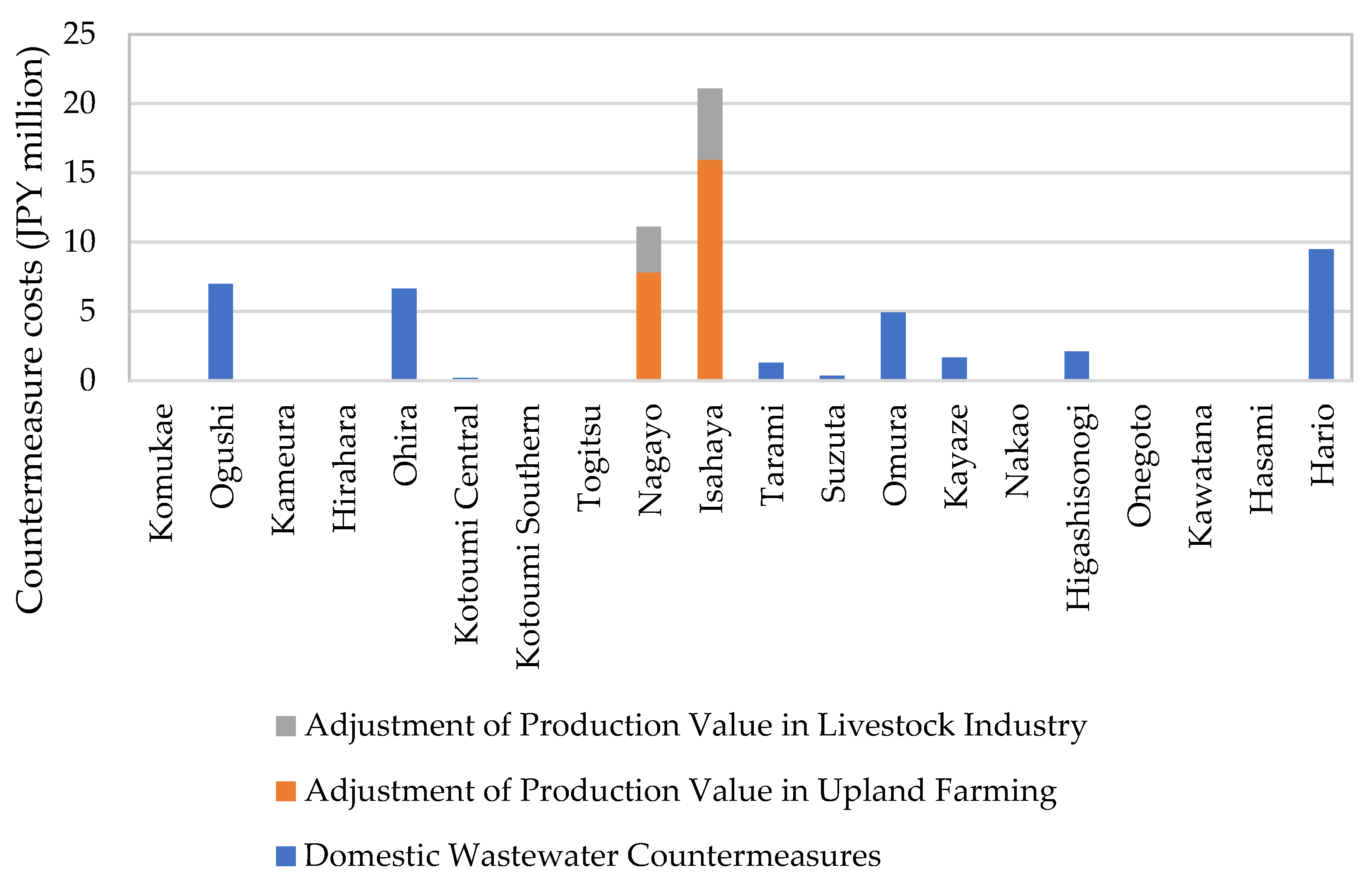
Figure 10 shows the costs and breakdown of policies implemented in each region under Scenario 2. The data suggests that production adjustment policies were effective in Nagayo and Isahaya, where nitrogen was reduced, whereas wastewater countermeasures were effective and efficient in other regions where COD or phosphorus was reduced. Notably, countermeasure costs were particularly high in regions where nitrogen (Nagayo, Isahaya) and phosphorus (Hario) were reduced. Therefore, introducing new technologies to recover and effectively utilize nitrogen and phosphorus in these regions could enable more efficient inflow management.

4.3. Research Value

The most important novelty of this study lies in introducing a new perspective—proper nutrient management (Scenario 2)—to complement the conventional one-dimensional evaluation of pollution load reduction measures. In this study, we quantitatively assess the economic and policy implications of this approach. As seen in recent years in the Seto Inland Sea and other areas, it has been indicated that excessive water purification potentially adversely affects fisheries. This study represents a pioneering attempt to use an economic model to concretely demonstrate sustainable water quality management approaches that also consider these negative aspects. Furthermore, it holds academic value in using an environmental economics approach to visualize the complex trade-off between “environmental conservation” and “regional economic activity” in enclosed sea areas, expressed as specific policy costs and changes in Gross Regional Product (GRP). Specifically, identifying the “tipping point” where pollution load reduction rates exceeding 12.3% cause countermeasure costs to surge sharply and GRP to decline significantly provides crucial insights for setting policy targets based on scientific evidence. The simulation results from this study can serve as a powerful decision-making support tool for formulating and evaluating concrete policies like Nagasaki Prefecture’s “Omura Bay Environmental Conservation and Restoration Action Plan.” The analysis shows that a management approach (Scenario 2) tailored to regional characteristics minimizes the impact on GRP. This approach also reduces countermeasure costs to approximately one-sixth (JPY 44.3 billion → 6.7 billion) compared to a uniform total quantity regulation (Scenario 1). This finding offers potentially crucial implications for designing highly cost-effective environmental policies. The simulation model developed in this study can be applied not only to Omura Bay but also to other enclosed coastal areas in Japan (such as Ariake Sea and Mikawa Bay) and overseas coastal regions facing similar issues by substituting input data like input–output tables and various statistical data. This enables the design of optimal environmental policies tailored to the socio-economic structures of each region.

4.4. Limitations

This study has several limitations, necessitating careful interpretation of its findings. The simulation model relies on a wide range of input variables and inherent mathematical simplifications. Consequently, the uncertainty associated with each input propagates and accumulates in the output results. Considering this uncertainty, discussing the consistency and credibility of the results is essential.

The core methodology employs linear programming (LP), which assumes a linear relationship among variables. While this linearity facilitates clear and interpretable trade-off analyses (e.g., identifying the “tipping point”), it may lead to cost underestimations or overestimations of feasibility at the solution boundaries. Therefore, absolute GRP and cost figures are best interpreted as relative indicators for policy comparison, not as precise absolute forecasts.

We use a single base year (2015) for input–output data to ensure model consistency. However, this restricts the model’s ability to capture long-term structural changes or unpredictable economic factors and thus limits the generality of the simulation results.

The model simplifies the pollutant–water quality relationship and uses a fixed river transport coefficient (Table A1) for natural purification. This method fails to adequately reflect complex physical processes (e.g., water circulation, seawater exchange, nutrient release from sediments) and, therefore, the estimated improvements in proportional water quality may not accurately reflect actual ecological outcomes. This limitation highlights the importance of integrating a more sophisticated hydrological model, as called for in Section 4.5: Future Challenges.

The examined policy measures are limited to existing government instruments, including sewage facility development, land conversion, and industrial subsidies. Proposing more effective and sustainable policies requires considering technological innovations and new environmental measures (e.g., natural regeneration or blue carbon introduction).

4.5. Future Challenges

One of the key challenges moving forward is further refining the model to better reflect real-world conditions. In this study, in Scenario 2, a proportional relation between the inflowing pollutant loads from the watershed into the bay and water quality indicators, such as environmental standards and measured values, was assumed for the sake of convenience when setting target pollutant load levels. However, a more sophisticated relationship between pollutant loads and water quality should be incorporated in the model considering factors such as water circulation within the bay and the rate of seawater exchange between the bay and the open sea.

Additionally, the pollutant load management policy was introduced under the assumption that water quality improvements would negatively impact the fishery industry. However, a quantitative analysis of how water quality improvements and eutrophication may affect fisheries might provide a more objective basis for evaluating the validity of this policy.

5. Conclusions

This study examined economic approaches for reducing and managing anthropogenic pollutant loads. The objective was to find a method that minimizes adverse socioeconomic effects, maintains the balance between the economy and the water environment, and enables the sustainable use of marine resources. Specifically, focusing on the Omura Bay watershed, we conducted simulations under two scenarios: Scenario 1, in which there is a total reduction in pollutant loads across the entire watershed, and Scenario 2, in which pollutant load targets are achieved based on regional water quality. We designed these simulations to determine the maximum feasible reduction in inflow pollutant loads without significantly affecting socioeconomic activities and to assess the feasibility of pollutant load management that considers the negative impacts of water quality improvement on the fishery industry while aligning with regional characteristics.

In Scenario 1, pollutant inflows into Omura Bay could be reduced by up to 12.7% while maximizing GRP. Additionally, based on GRP variations, we identified a reduction of 12.3% as an appropriate level that could be achieved without harming socioeconomic activities.

Achieving this requires a total countermeasure cost of JPY 33.4 billion over 20 years. The breakdown of this cost is as follows: JPY 14.0 billion for the development of domestic wastewater treatment facilities; JPY 10.5 billion for the fallow farmland policy; JPY 0.9 billion for the fallow paddy field policy; JPY 4.8 billion for livestock production adjustments; JPY 1.9 billion for fisheries production adjustments; and JPY 1.2 billion for rice production adjustments. These findings suggest that within the Omura Bay watershed, significantly reducing pollutant inflows without at least some impact on industries is impossible under existing methods.

Scenario 2 identified a pollutant emission management policy where pollutant loads would be reduced in areas with poor water quality and appropriately increased in areas with good water quality, without significantly affecting socioeconomic activities in the Omura Bay watershed. In this scenario, GRP remained largely unchanged, and the countermeasure cost was relatively low at JPY 6.7 billion over 20 years, making it a more economically efficient alternative to a uniform total load reduction approach. Additionally, this scenario clarified how policies tailored to regional characteristics and their associated costs should be appropriately allocated across different areas.