Article

AI-Based Time-Series Ensemble Approach Coupled with a Hydrological Model for Reservoir Storage Prediction in Korea

1
Major of Geomatics Engineering, Division of Earth Environmental System Sciences, Pukyong National University, Busan 48513, Republic of Korea
2
Research Institute for Geomatics, Pukyong National University, Busan 48513, Republic of Korea
3
Department of Water Resources, Graduate School of Water Resources, Sungkyunkwan University, Suwon 16419, Republic of Korea
4
Department of Geoinformatic Engineering, Inha University, Inchon 22212, Republic of Korea
5
Department of Applied Plant Science, Chonnam National University, Gwangju 61186, Republic of Korea
*
Author to whom correspondence should be addressed.
Water 2025, 17(22), 3296; https://doi.org/10.3390/w17223296
Submission received: 18 October 2025 / Revised: 13 November 2025 / Accepted: 15 November 2025 / Published: 18 November 2025

Abstract

In regions like South Korea, erratic seasonal rainfall creates a dual vulnerability for agricultural reservoirs: rapid storage increases during the rainy season risk flooding and structural damage, while insufficient storage during dry periods leads to inadequate irrigation. Accurate reservoir storage prediction is therefore crucial. It enables pre-emptive storage and release planning, ensuring stable reservoir management and efficient water utilization despite unpredictable weather conditions. AI-based prediction offers a solution to the aforementioned challenges. However, previous studies had two key limitations: (1) they could not account for inflow and outflow variables in reservoirs that do not provide these data, and (2) they relied on Recurrent Neural Network (RNN) models with a recursive prediction mechanism, leading to decreased accuracy as the lead time increased. To overcome this, we propose a framework that simulates reservoir inflow and outflow using a rainfall–runoff hydrological model and utilizes these variables as inputs for time-series AI models. We then predict the storage rate using a Bayesian Model Averaging (BMA) ensemble of Long Short-Term Memory (LSTM), Gated Recurrent Unit (GRU), and Temporal Fusion Transformer (TFT) models, which resulted in a substantial accuracy improvement. The Mean Absolute Error (MAEs) for 1-day, 2-day, and 3-day ahead predictions were 0.820%p, 1.339%p, and 1.766%p, respectively, with corresponding correlation coefficients of 0.994, 0.987, and 0.980. This framework maintains high accuracy even as the lead time increases. The proposed framework can predict reservoir storage rates with high accuracy, even for reservoirs characterized by irregular seasonal rainfall patterns and a lack of explicit inflow/outflow data, thus contributing to more effective reservoir operation.

1. Introduction

In recent years, the intensification of global climate change has led to more frequent and severe droughts and floods, underscoring the growing importance of effective water resource management using reservoirs and dams [1,2]. In regions such as South Korea, where rainfall patterns are highly irregular across seasons, agricultural reservoirs experience rapid storage increases during the rainy season, making them vulnerable to flooding and structural damage. Conversely, during dry periods, insufficient storage often results in inadequate irrigation water for downstream agricultural areas, posing significant challenges to water management [3,4,5,6]. Accurate reservoir storage prediction can, therefore, enable pre-emptive planning for storage and release operations, ensuring stable reservoir management and efficient water utilization even under erratic weather conditions [7].
Traditional physical approaches to reservoir storage prediction rely on hydrological principles and water balance equations to simulate reservoir operations [8,9]. Although these models provide physically interpretable parameters that facilitate understanding of the underlying processes [10,11], they require extensive computational resources and are subject to uncertainties arising from input data errors and structural assumptions [12,13,14,15].
As an alternative, data-driven approaches utilizing artificial intelligence (AI) have demonstrated higher predictive accuracy and computational efficiency compared to physical models. Time-series models such as the Autoregressive Integrated Moving Average (ARIMA) model have been employed; however, vanilla ARIMA is limited in multivariate forecasting, making it difficult to incorporate external variables such as precipitation or evaporation [16,17,18,19]. The Support Vector Machine (SVM) model supports multivariate forecasting by considering multiple hydrological factors [20,21,22]. In addition, numerous studies have explored neuro-fuzzy systems [22,23,24,25,26], tree-based models [27,28], and artificial neural networks (ANNs) [28,29,30,31] for storage prediction.
In more recent years, deep learning models have gained prominence in reservoir storage forecasting. Recurrent Neural Network (RNN) models such as Long Short-Term Memory (LSTM) and Gated Recurrent Unit (GRU) as well as Convolutional Neural Network (CNN) models have shown superior predictive performance compared to traditional machine learning methods [32,33,34,35,36,37]. Furthermore, hybrid models combining physical and AI-based approaches [38], modified architectures such as CNN–LSTM and CNN–Attention–LSTM [39], and ensemble learning strategies [40] have further improved forecast accuracy.
However, previous AI studies have been limited to the use of meteorological and storage data, neglecting key hydrological components such as inflow and outflow, which are influenced by watershed characteristics and reservoir operation rules [41]. Essential variables for reservoir storage prediction include storage, precipitation, evaporation, inflow, and outflow [8]. While precipitation and evaporation can be obtained from meteorological observations or numerical models, inflow depends on catchment hydrology and is often unavailable for many reservoirs. Outflow, in contrast, is largely determined by human-controlled reservoir operation rules, making it difficult to quantify without dedicated monitoring systems.
Several previous studies have utilized inflow and outflow data in their research; however, these data were collected by the researchers themselves [21,25,26,27,31,39]. In South Korea, while a small number of reservoirs managed by the Korea Water Resources Corporation (K-water) provide inflow and outflow data, the majority—approximately 17,100 agricultural reservoirs managed by the Korea Rural Community Corporation (KRC)—do not. This presents a significant limitation for studies involving streamflow or storage prediction [42,43].
RNN-based models such as LSTM and GRU have been commonly employed for multi-step-ahead forecasting. Both models address the vanishing gradient problem inherent in traditional RNNs through memory cells and gating structures, allowing them to capture long-term dependencies more effectively. However, due to their recursive prediction mechanism—where the output at time t becomes the input for time t + 1—these models suffer from error accumulation, leading to biased predictions as the forecast horizon increases [44,45]. To address this limitation, estimating inflow and outflow using a rule-based rainfall–runoff model such as Three-Tank Model (3TM) can enhance the accuracy of reservoir storage predictions by incorporating the simulated inflow and outflow data into RNN-based models [41].
Moreover, the Temporal Fusion Transformer (TFT) has recently emerged as a powerful alternative to the existing RNN architectures. As a transformer-based deep learning model, TFT is equipped with dedicated temporal processing paths and an internal attention mechanism designed to handle multivariate time-series data efficiently. By dynamically adjusting the importance of past and future inputs and providing interpretable outputs, TFT achieves superior mid-term prediction accuracy compared to the existing RNN models and enables objective evaluation of variable importance through attention mechanisms [46].
The first objective of this study is to enhance reservoir storage prediction accuracy for KRC-managed agricultural reservoirs that lack inflow and outflow data. This is achieved by simulating daily inflow and outflow using 3TM and incorporating them as input features in AI time-series prediction models. The contribution of these variables to storage prediction is quantified using explainable AI (XAI) techniques applied to the TFT model.
The second objective is to predict agricultural reservoir storage rates using the TFT model—capable of superior temporal feature learning—and to compare its performance with the generic RNN-based models (LSTM and GRU) to verify the predictive advantage of TFT. Using time-series AI models, reservoir storage rates were forecasted 1, 2, and 3 days ahead, and the predictive performance of each model was quantitatively evaluated using several performance metrics.
Finally, to further improve prediction accuracy, this study develops an ensemble model combining LSTM, GRU, and TFT, leveraging the nonlinear feature extraction capabilities of LSTM and GRU together with the temporal attention strengths of TFT to achieve higher prediction accuracy than any single model.

2. Materials and Methods

2.1. Overview

Figure 1 summarizes the overall workflow of this study. First, we separated the periods with zero discharge from those with nonzero discharge based on the patterns of the water level time series, distinguishing between the cultivation and non-cultivation periods, as well as the flood control periods. The inflow can be estimated using the water balance equation only for the periods when the discharge is zero. Second, the optimized 3TM is driven for both zero- and nonzero-discharge periods using meteorological inputs. Through this process, daily inflow can be simulated for the entire period, and the reservoir outflow during nonzero-discharge periods is estimated using the water balance equation. Third, the simulated inflow and outflow from the 3TM, together with precipitation, evaporation, and the temporal variable Julian day, are used as input features for training and optimizing multiple AI-based reservoir storage rate prediction models. Finally, the performance of the AI models is evaluated using statistical indicators such as mean bias error (MBE), mean absolute error (MAE), and correlation coefficient (CC), and a Bayesian Model Averaging (BMA) ensemble approach is employed to further improve the accuracy of reservoir storage rate predictions.

2.2. Study Area

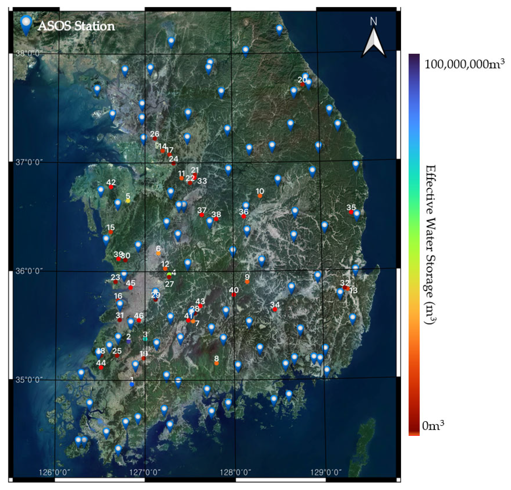
This study was conducted on the 46 agricultural reservoirs managed by the KRC that are equipped with water level gauges and provide water level and storage rate information (Table 1). These reservoirs do not provide inflow and outflow data; therefore, in this study, inflow and outflow were estimated using 3TM based on reservoir operation rules and subsequently used as input variables for reservoir storage rate prediction [42]. Figure 2 shows the spatial distribution of the study reservoirs. In South Korea, mountainous terrain is predominantly distributed in the eastern region, making it less suitable for agriculture, whereas extensive plains lie to the west of approximately 127 °E, where agricultural activities are concentrated. Consequently, most of the study reservoirs are located in the southwestern plains of Korea, where farming is more active [47].

2.3. Dataset

2.3.1. Reservoir Data

In this study, daily water level and storage rate data from 2013 to 2024 (a 12-year period) were utilized for the 46 agricultural reservoirs managed by the KRC with the largest effective storage capacities. The water level data were used, together with the operational rules of agricultural reservoirs, to distinguish periods of zero discharge from those with nonzero discharge, while the storage rate data served as the target variable in the time-series AI models. Among approximately 17,100 reservoirs managed by KRC, about 3400 are equipped with water level monitoring systems that provide daily time-series information such as water level and storage rate, as well as facility characteristics including effective storage capacity and catchment area. However, these reservoirs do not provide inflow or outflow data [37,42,48]. In addition, some reservoirs constructed during the 1960s and 1970s are aging and thus vulnerable to structural damage during heavy rainfall periods, highlighting the necessity of AI-based water storage prediction systems for efficient reservoir management.

2.3.2. Meteorological Data

Meteorological data were obtained from the Automated Surface Observing System (ASOS) operated by the Korea Meteorological Administration (KMA) [49]. ASOS is a nationwide ground-based observation network consisting of 105 stations that monitor various meteorological variables, such as air temperature, humidity, precipitation, solar radiation, and evaporation. In this study, data from the nearest ASOS station to each reservoir were used. The minimum distance between a reservoir and its nearest ASOS station was 1.91 km (Gabuk), while the maximum distance was 38.17 km (Cheongho). Among the variables provided by ASOS, precipitation and evaporation were employed both as input variables for the reservoir storage prediction models and for the water balance equation for 3TM. Meanwhile, mean wind speed, solar radiation, relative humidity, and mean temperature were used as input variables for optimizing 3TM. Because evaporation is measured using a Class A evaporation pan, a pan coefficient of 0.6 was applied to convert pan evaporation to actual evaporation [50].

2.4. Rule-Based Rainfall–Runoff Process

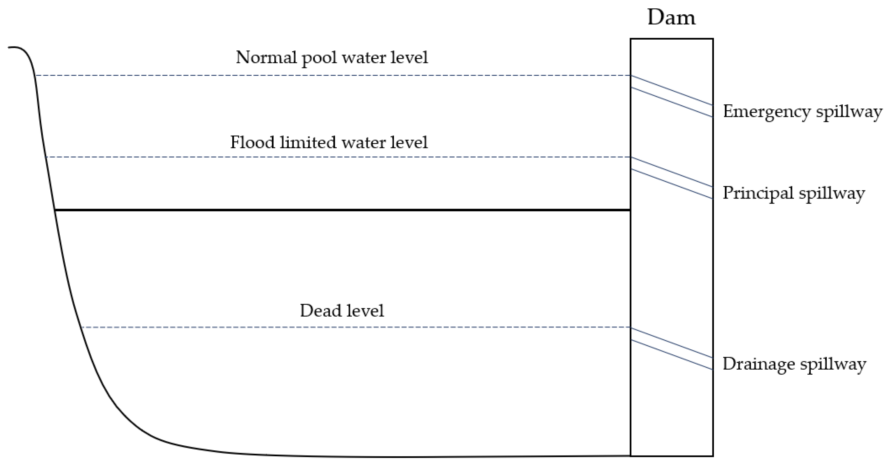
The methodology for simulating reservoir inflow and outflow based on rule-based rainfall–runoff process of agricultural reservoirs was proposed by Song et al. [41], and Figure 3 provides a summary of this approach. The key concept is to transform the reservoir water balance equation—originally an indeterminate system due to the two unknown variables of inflow and outflow—into a determinate form for specific periods by applying reservoir operation rules, such as storage and release schedules during the flood control and cultivation seasons. Using these operational rules, the entire study period can be divided into zero-discharge and nonzero-discharge periods. The water balance equation can be applied only to the zero-discharge periods to estimate reservoir inflow. The inflow derived from these zero-discharge periods is then used to calibrate 3TM, and the optimized 3TM is subsequently employed to simulate inflow for the nonzero-discharge periods. Once inflow for all periods is simulated, the reservoir outflow for each period is finally estimated through the water balance equation. The simulated inflow and outflow are then used as input features for the AI-based reservoir storage rate prediction models.

2.4.1. Reservoir Water Balance

The reservoir water balance equation can be expressed as Equation (1) [7,41,51,52,53,54,55]. In this equation, S represents the reservoir storage (m3), RI denotes the inflow from the surrounding watershed (m3/s), R is the direct rainfall on the reservoir surface (m3/s), E is the evaporation from the reservoir surface (m3/s), G is the infiltration to groundwater through the reservoir bed (m3/s), and RO represents the outflow through the reservoir spillway (m3/s). The groundwater infiltration term (G) was not considered in this study because it has a negligible influence on the water balance and cannot be directly measured.
d S d t = ( RI + R ) ( E + G + RO )

2.4.2. Reservoir Operation Rule

RO can be classified according to its discharge purpose into three types: irrigation discharge through the drainage spillway, flood-control discharge through the principal spillway to maintain the flood control level, and emergency discharge through the emergency spillway to prevent structural damage [7,41,53] (Figure 3). During the cultivation period, agricultural reservoirs release water through the drainage spillway to supply irrigation water to downstream farmlands. In the non-flood season, discharge occurs solely for irrigation purposes. During the flood control period, when the reservoir water level exceeds the flood control level, water is released through the principal spillway to regulate storage under rapidly increasing inflow conditions and to prevent damage to the structures. The emergency spillway is activated when the reservoir water level reaches the full supply level, serving as an outlet to prevent structural damage by releasing excess water beyond the storage capacity. Based on these operational rules, periods with zero discharge and those with positive discharge can be distinguished over the entire simulation period. Further details on the reservoir operation rules are provided in Appendix A.

2.4.3. Inflow Reconstruction

Using the reservoir operation rules, the simulation period can be divided into intervals with zero discharge and those with positive discharge. The inflow during the zero-discharge periods is calculated using Equation (2). Here, R I R O = 0 represents the reservoir inflow during periods when RO equals zero. Since this inflow is derived solely from observed data using Equation (2), it is regarded as an observed value of 3TM. The optimization of 3TM is then performed by comparing R I R O = 0 obtained from Equation (2) with the simulated watershed runoff generated by the model. The optimized model is subsequently applied to simulate the reservoir inflow during periods with positive discharge, denoted as R I R O > 0 . Finally, the total inflow throughout all periods can be estimated using Equation (3).
R I R O = 0 = d S d t R + E
R I = R I R O = 0 + R I R O > 0

2.4.4. Outflow Reconstruction

Once RI is estimated for all periods, the discharge for each period can be calculated using Equation (4), which is a rearranged form of Equation (1).
R O = d S d t + R I + R E

2.4.5. Three-Tank Model Simulation

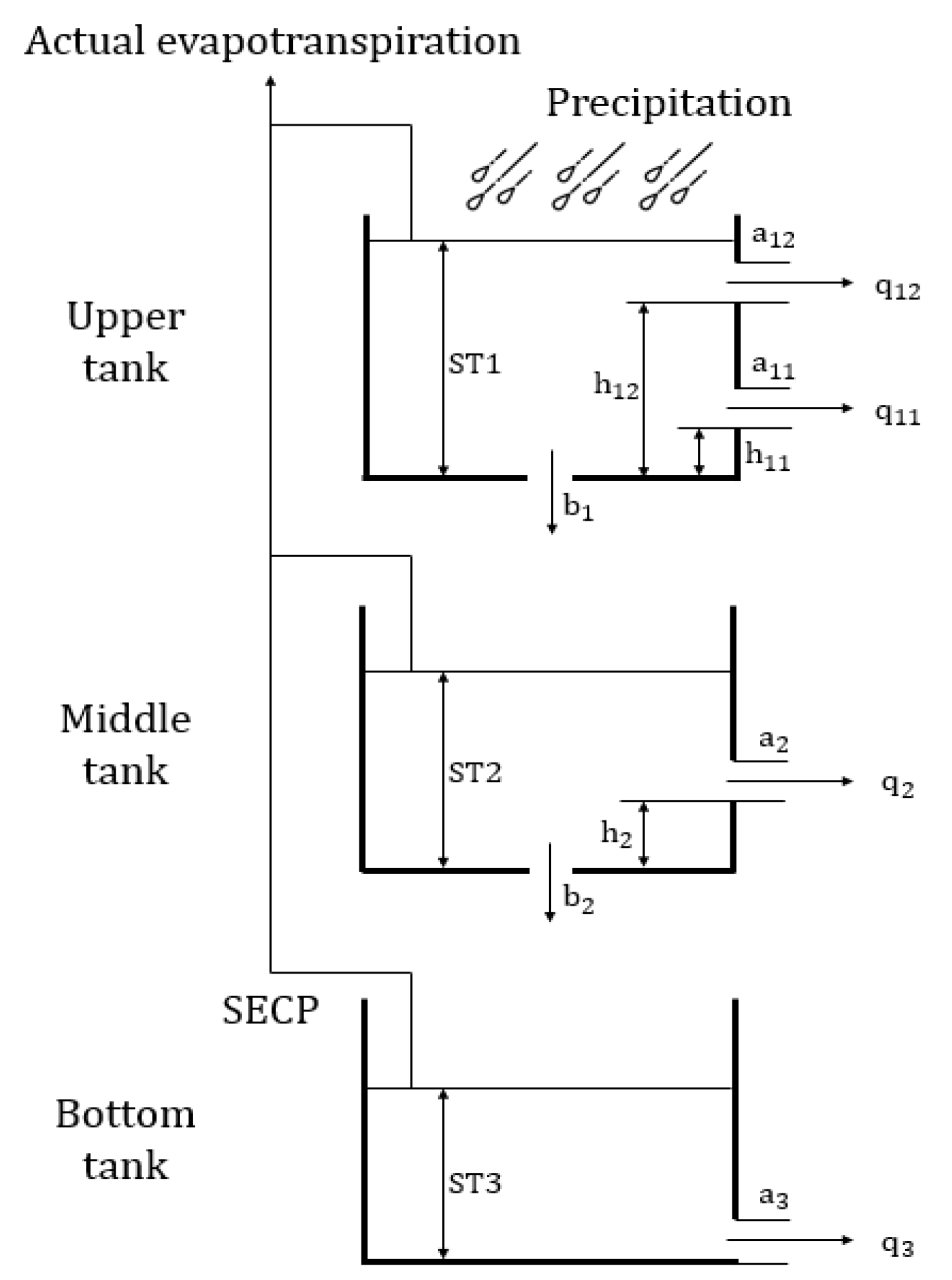
In this study, the 3TM was employed to simulate the watershed runoff that includes the reservoir. This model has proven to be an effective tool for representing hydrological processes in East Asian regions characterized by complex topography, such as Korea, Japan, and Taiwan [56,57,58]. The 3TM consists of three vertically arranged tanks: the upper tank represents surface runoff, the middle tank represents subsurface runoff, and the lower tank represents baseflow (Figure 4).
The physical meaning and possible range of each parameter in 3TM are summarized in Table 2. a denotes the outflow coefficient for each outlet, h represents the storage capacity of each tank, and b indicates the outflow coefficient for percolation to the lower tank. The actual evapotranspiration (AET) required for 3TM simulation is calculated using Equation (5).
A E T = K c ·   P E T · 1 e x p ( S E C P · S T S )
where K c represents the crop coefficient [52,59], PET denotes the potential evapotranspiration calculated using the Penman–Monteith (PM) method [59], SECP is soil evaporation compensation parameter, and STS indicates the total streamflow of the watershed (m3/s). They are calculated using Equations (6), (7) and (8), respectively.
K c ( m o n t h ) = f · F m o n t h + p · P m o n t h + u · U m o n t h + o · O m o n t h 100
where f denotes the fraction of forested area within the watershed, p the fraction of paddy fields, u the fraction of upland fields, and o the fraction of other land cover types. Correspondingly, F, P, U, and O represent the crop coefficients for forest, paddy field, upland field, and other land cover types for the given month. The overall crop coefficient is expressed as a linear combination of the crop coefficients for each land cover type.
P E T = 0.408 R n G + γ ( 900 T + 273 ) u 2 ( e s e a ) + γ ( 1 + 0.34 u 2 )
where R n represents the net radiation at the crop surface (MJ m−2 day−1), G is the soil heat flux (MJ m−2 day−1), T is the surface air temperature (°C), u 2 denotes the wind speed measured at 2 m above the ground (m s−1), e s is the saturation vapor pressure (kPa), e a is the actual vapor pressure (kPa), Δ represents the slope of the vapor pressure curve (kPa °C−1), and γ is the psychrometric constant (kPa °C−1).
S T S = S T 1 + S T 2 + S T 3
where ST1 represents the outflow from the upper tank (m3/s), ST2 represents the outflow from the middle tank (m3/s), and ST3 represents the outflow from the lower tank (m3/s).

2.4.6. Optimization and Performance Evaluation

For the optimization of 3TM, the Non-Dominated Sorting Genetic Algorithm II (NSGA-II) was employed, using Nash–Sutcliffe Efficiency (NSE) and N S E l o g as the objective functions (Table 3) [60]. Since NSE squares the difference between simulated and observed discharge, it gives greater weight to high-flow conditions, whereas N S E l o g , due to the logarithmic transformation, is more sensitive to low-flow conditions [61,62]. Both metrics are generally recommended to have values greater than 0.5 to indicate satisfactory model performance [63]. The objective functions used for optimizing 3TM were normalized to a range between –1 and 1, as expressed in Equation (9) [41,54,61,62]. C′ denotes the normalized statistical value ranging from –1 to 1, and C represents the original statistical value.
C = C 2 C
Before being used as input features in the AI model, the inflow and outflow simulated by 3TM were evaluated through accuracy and sensitivity analyses. For the accuracy assessment, the NSE and N S E l o g statistics listed in Table 2 were employed, and the analysis was conducted only for R I R O = 0 . Since R I R O = 0 was estimated solely from observed data on reservoir storage, precipitation, and evaporation, it was regarded as an observed value, allowing the evaluation of model accuracy. In contrast, R I R O > 0 lacked corresponding observational data, and thus no accuracy analysis was performed for this case. Similarly, for reservoir discharge, periods with zero discharge were considered observed values based on reservoir operation rules, whereas periods with positive discharge had no observations available; therefore, accuracy analysis was not conducted for discharge.
Sensitivity analysis was performed using the Generalized Likelihood Uncertainty Estimation (GLUE) method. The behavioral range of 3TM was defined as cases where both NSE and N S E l o g were between 0.6 and 0.9. For inflow, the sensitivity analysis was separately conducted for periods with zero and positive discharge. For outflow, sensitivity analysis was performed only for periods with positive discharge, as zero discharge periods were treated as observed values according to the reservoir operation rules. Among the behavioral simulations within the defined range, the parameter combination that maximized the joint likelihood of NSE and N S E l o g was ultimately selected to simulate inflow and outflow, which were then used as input features in the reservoir storage AI model.

2.5. Time-Series AI Models

To build time-series AI models, we used the input features such as past reservoir storage rates, inflow, outflow, precipitation, evaporation, and Julian day. The Julian day is represented as the cosine-transformed value of a periodic function with a cycle of 365 days (or 366 in leap years) to account for seasonal periodicity. RNN models such as LSTM and GRU as well as Transformer model such as TFT were employed to compare the predictive performance and to perform BMA ensemble. The optimization of the storage rate prediction models was performed using the Optuna library in Python 3.10. The optimization process in Optuna is based on Bayesian optimization, which explores the predefined hyperparameter space to efficiently find the combination that minimizes the validation loss. To effectively utilize all reservoir datasets and improve the model’s generalization capability across different sites, we developed separate, unified (pooled) models for the LSTM, GRU, and TFT architectures, utilizing the data from all 46 reservoirs.

2.5.1. Recurrent Neural Network Model

The vanilla RNN, which preceded LSTM and GRU, was originally designed to process sequential or time-series data by storing information from previous time steps in the hidden state and using it to predict subsequent values, thereby reflecting temporal dependencies. However, vanilla RNNs suffer from the vanishing gradient problem caused by repeated differentiation of the tangent hyperbolic (tanh) function during backpropagation, leading to difficulty in learning long-term dependencies [64,65].
LSTM was developed to overcome these limitations of the vanilla RNN by introducing a structure composed of a forget gate, input gate, output gate, and cell state, which together regulate the flow of input and output information. During backpropagation, the derivative of the tanh function—the main source of vanishing gradients—is computed only once, effectively mitigating the vanishing gradient problem [66] (Figure 5). GRU, on the other hand, is a simplified variant of the LSTM architecture that uses only two gates—the update gate and reset gate—to control input and output [67]. While LSTM tends to achieve higher accuracy in complex tasks, GRU requires fewer parameters and trains at a faster rate due to its simplified structure, often yielding performance comparable to that of LSTM across many tasks [68,69].
The memory cell is the core of the LSTM network, responsible for carrying important information throughout the time series. Its update is determined by the following equation:
C t =   F t C t 1 + I t C ¯ t
where C t is the cell state at the current time step, C t 1 is the cell state at the previous time step, and represents element-wise multiplication.
The input gate primarily functions to control the flow of new information into the memory cell. It consists of two parts: a Sigmoid layer, which decides which values to update, and a tanh layer, which creates a new candidate vector to be added to the memory cell. The main equations are as follows:
I t =   σ ( W t h t 1 , x t + b t
C ¯ t = t a n h ( W C h t 1 . x t + b C
where Equations (11) and (12), I t is the output of the input gate, and σ is the Sigmoid activation function, which produces a value between 0 and 1 to indicate how much of the previous time step’s cell state should be retained. C ¯ t is the new candidate value to be added to the cell state. W t and W C are the weight matrices corresponding to the input gate and the candidate value vector, respectively. b i and b c the bias terms for the input gate and the candidate value vector, respectively.
The forget gate controls the amount of information discarded from the cell state. It decides which information to retain by observing the current input and the previous hidden state:
F t = σ ( W f h t 1 . x t + b f
where F t is the output of the forget gate at time step t. W f is the weight matrix of the forget gate, h t 1 is the hidden state of the previous time step, x t is the input at the current time step, and b f is the bias term of the forget gate.
The output gate controls the flow of information from the memory cell to the hidden state. It utilizes the Sigmoid function, observing the current input and the previous hidden state, to determine which information can be output as the hidden state of the current time step. After processing the memory cell through the tanh function, its output is multiplied by the output gate to obtain the final hidden state, h t .
O t = σ ( W o h t 1 . x t + b o
h t = O t t a n h ( C t )
where O t is the output of the output gate at time step t. W o is the weight matrix of the output gate. b o is the bias term for the output gate.
The update gate of the GRU primarily functions to control how much of the previous hidden state should be retained versus how much new information should be incorporated. It consists of a Sigmoid layer that outputs values between 0 and 1, determining the degree of update for each element of the hidden state. The reset gate controls how much of the past information to forget. It also consists of a Sigmoid layer that decides which parts of the previous hidden state should be ignored when computing the candidate hidden state:
Z t = σ ( W z h t 1 . x t + b z
R t = σ ( W r h t 1 . x t + b r
where Z t and R t are the output of update gate and reset gate at time step t, respectively. W z and W r are the weight matrices of update gate and reset gate. b z and b r are their bias term of update and reset gate.

2.5.2. Transformer Model

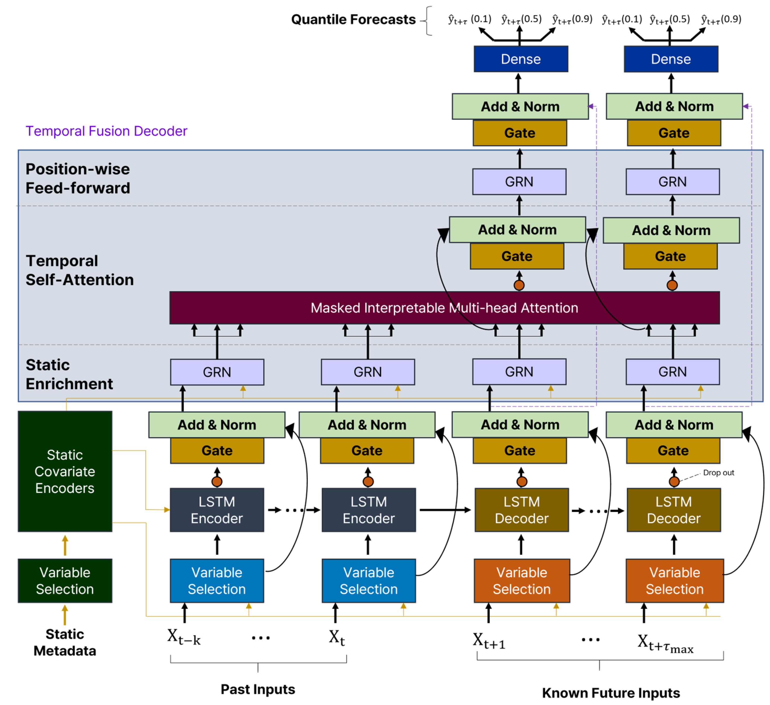
We employed TFT, a transformer-based time series AI model, to improve the predictive accuracy of conventional RNN models [46]. Figure 6 illustrates the prediction process of the TFT model. TFT processes input variables by categorizing them into static inputs, observed inputs, and known inputs. Regardless of variable type, all inputs first pass through the variable selection network, which distinguishes between important and less important variables at each time step.
TFT model utilizes LSTM encoder and decoder cells to sequentially process past inputs and learn short- and medium-term temporal patterns. The static enrichment network then integrates static information into the temporally processed outputs from the LSTM, enriching the temporal context and enhancing prediction accuracy. The temporal multi-head attention mechanism emphasizes important time steps from the past, thereby strengthening long-term dependencies. In the position-wise feed-forward network, the outputs from the attention mechanism are nonlinearly transformed; this stage incorporates layer normalization and residual connections, ensuring stable training even in deeper architectures.
Moreover, the TFT performs its prediction through the output of a dense layer, enabling simultaneous forecasting across multiple future time steps. This approach provides superior predictive accuracy compared to RNN-based time series models. In addition, the attention mechanism within TFT allows for the quantitative evaluation of variable importance among the input features used in prediction. Using this mechanism, the importance of variables contributing to the reservoir storage prediction was assessed.

2.6. Baysian Model Averaging Ensemble

BMA is a probabilistic forecasting technique based on Bayesian statistical theory that converts deterministic predictions from individual models into probabilistic forecasts and integrates predictions from multiple sources. This method assigns weights to each model according to its posterior probability of best explaining the observed data and derives the overall posterior probability density function (PDF) of a variable by taking the weighted average of the conditional PDFs from each model (Equation (18)) [70,71].
p ( y | M 1 , M 2 , M k ) = k = 1 K w k · h k ( y | M k )
where y denotes the target variable to be predicted, Mk represents the prediction from the k-th model, and wk is the weight corresponding to the posterior probability that the k-th model is the most suitable for prediction, subject to the condition k = 1 K w k = 1 . h k ( y | M k ) denotes the conditional probability density function of variable y given the prediction Mk from the k-th individual model.

3. Results

3.1. Data Analysis

3.1.1. Water Storage Rates

We first examined the annual storage rate pattern of an agricultural reservoir (Figure 7). During the non-cultivation period, water is stored close to full capacity (100% storage rate) in preparation for irrigation discharge during the cultivation period. As irrigation water is released to downstream agricultural areas during the cultivation season, the storage rate decreases sharply [7,41]. Subsequently, during the flood control period, the storage volume increases rapidly due to increased rainfall on the reservoir surface and inflow from the surrounding watershed, coupled with reduced irrigation demand in the downstream areas. To prevent structural damage and flood inundation, storage and release are alternated based on the flood control level. After the cultivation period ends, the storage volume is increased again in preparation for the next cultivation season.
To verify whether the target reservoirs follow the seasonal pattern of agricultural reservoirs shown in Figure 7, we analyzed the monthly average storage, standard deviation, and mean of daily difference (MADD) of the target reservoirs (Table 4). Examining the monthly statistics of the storage volume, the average storage rate from January to April, the non-cultivation period, ranged from 76.9% to 84.4%, indicating a storage rate between 70% and 80%. However, in May and June, when the cultivation period begins, the storage rate gradually decreased to 76.2% and 55.0%, which can be attributed to the release of irrigation water to the downstream agricultural areas. For the flood control period in July and August, the average storage rate was higher, at 62.4% and 62.5%, due to the influence of rainfall, compared to May and June. From October to December, corresponding to the non-cultivation period, the average storage rate increased to 68.9%, 71.0%, and 74.4%, likely due to the storage of water in preparation for the next year’s irrigation discharge. The standard deviation was larger during the cultivation period, ranging from approximately 17% to 19%, compared to the non-cultivation period, which showed relatively smaller variations in storage. In July and August, corresponding to the flood control period, the MADD values were 1.25% and 0.97%, respectively, which were higher than those of the non-cultivation months with MADD values below 0.5%. This can be attributed to the repeated storage and release during the flood control period.
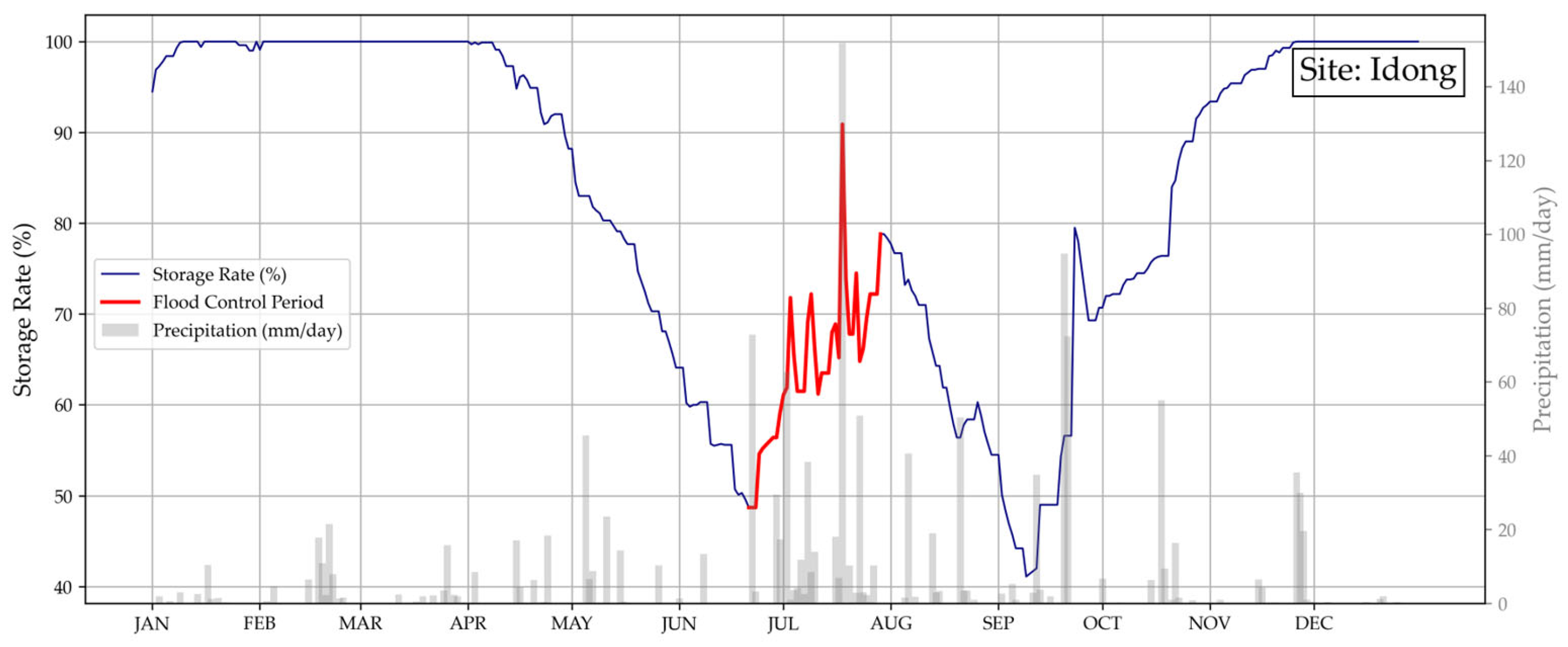
Figure 8 shows the 2024 storage rate graph for the Idong Reservoir, located in Gyeonggi Province. Starting from mid-April, the storage rate decreases as irrigation water is released. During the flood control period, indicated by the red line, the storage rate increases due to increased rainfall and inflow from the surrounding watershed. In this period, storage and release are alternated to prevent damage to the facility. From October, after the crop harvest, the storage rate increases in preparation for the next year’s irrigation release, eventually reaching 100%. This aligns with the seasonal storage rate pattern of agricultural reservoirs, confirming the appropriateness of applying the agricultural reservoir operation rules that distinguish between periods with zero and non-zero discharge.

3.1.2. Meteorological Data

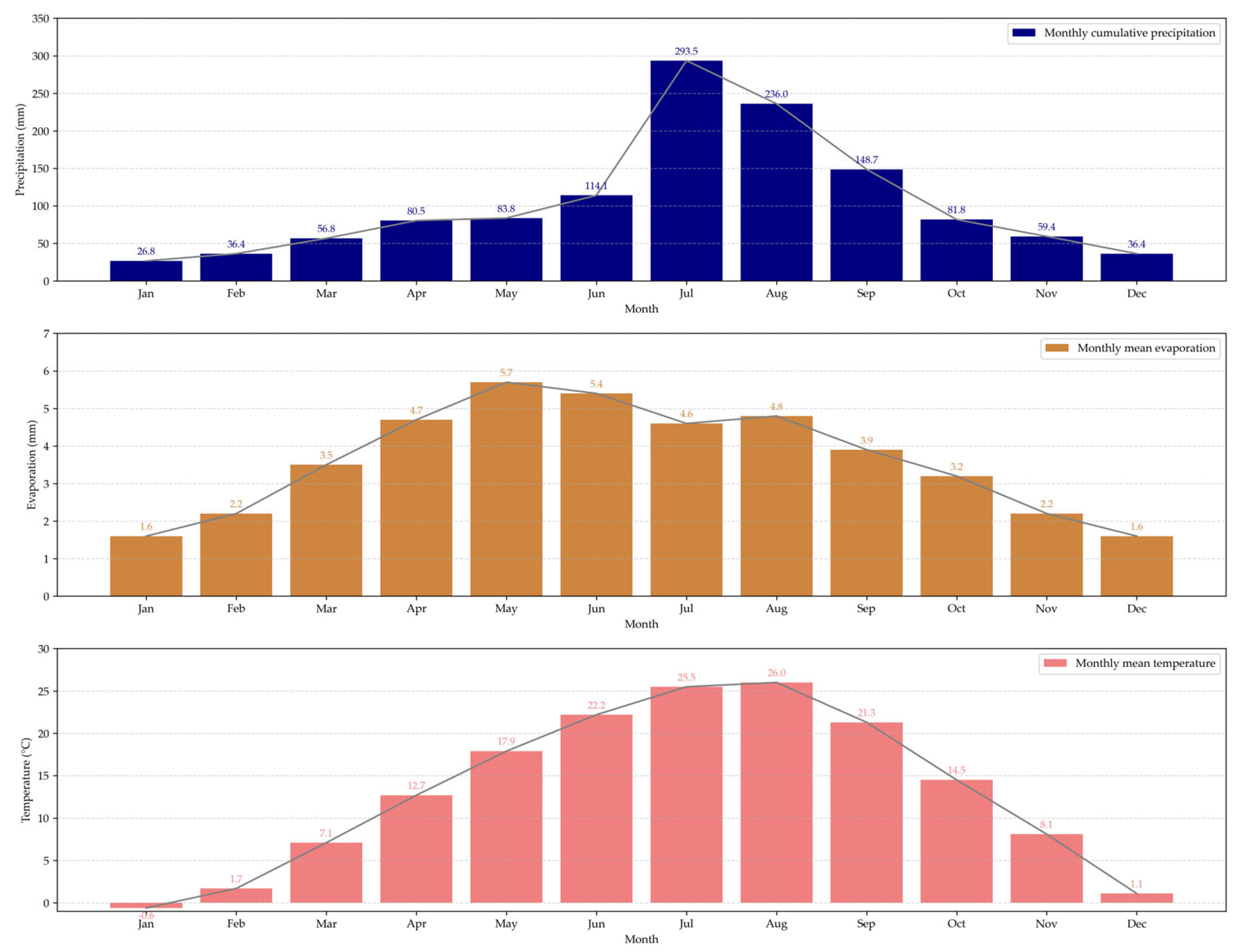
Figure 9 shows the monthly cumulative precipitation, mean evaporation, and mean temperature, averaged over the 46 reservoirs, using data from the nearest ASOS stations from 2013 to 2024. South Korea is geographically located in the temperate climate zone of the mid-latitudes, where distinct four seasons—spring, summer, fall, and winter—are observed. During the rainy season from June to August, a significant portion of the annual precipitation is concentrated. For June, July, and August, the cumulative precipitation recorded was 114.1 mm, 293.5 mm, and 236.0 mm, respectively, accounting for 51.3% of the total annual precipitation of 1254.2 mm. Evaporation was also higher in June, July, and August, with values of 5.4, 4.6, and 4.8 mm, respectively, compared to other months. The mean temperature was also elevated during these months, measuring 22.2 °C, 25.5 °C, and 26.0 °C, respectively. Precipitation is a key factor influencing the seasonal changes in storage rates, and this highlights the importance of water resource management during the rainy season and the appropriateness of applying reservoir operation rules related to flood control for agricultural reservoirs.

3.1.3. Inflow and Outflow

We analyzed the sensitivity of inflow and outflow simulated by 3TM for 46 reservoirs (Table 5). For periods with zero discharge, the inflow sensitivity ranged from a minimum of 0.113 mm/day to a maximum of 1.036 mm/day. For periods with non-zero discharge, the sensitivity ranged from a minimum of 0.232 mm/day to a maximum of 1.507 mm/day. The outflow sensitivity ranged from a minimum of 0.111 mm/day to a maximum of 0.853 mm/day. Both inflow and outflow sensitivities were similar to those of the existing work [41].
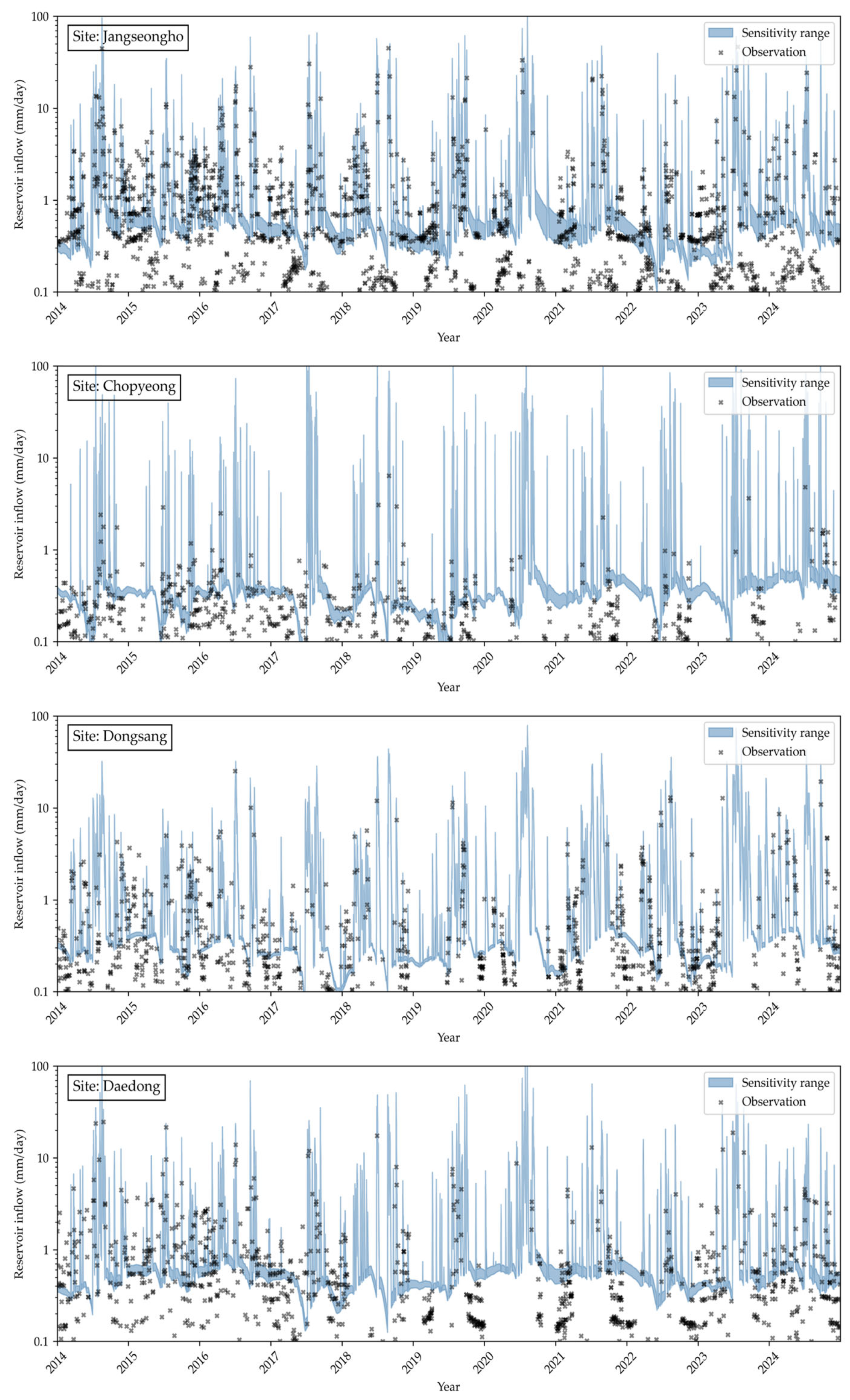
Figure 10 shows the time series of inflow sensitivity for Jangseongho, Chopyeong, Dongsang, and Daedong Reservoirs, ranging from 2014 to 2024. Among the four reservoirs, Jangseongho is the largest with a usable storage of 99,707,200 m3, making it the second-largest reservoir in the study area. Chopyeong and Dongsang reservoirs are medium-sized, with usable storage of 13,853,200 m3 and 11,241,100 m3, ranking 22nd and 27th in usable storage, respectively. Daedong Reservoir is the smallest, with a usable storage of 7,502,100 m3, ranking third in the study area for the smallest usable storage. The blue shading in Figure 10 represents the uncertainty range based on 3TM simulations, while the black dots represent the observed inflow during periods with zero discharge. In some summer high-flow periods, where inflow is concentrated due to rainfall, the uncertainty range is wide, but overall, the uncertainty range remains narrow. In low-flow periods between 0.1 mm/day and 1 mm/day, the observed values fall outside the sensitivity range, but most observed values lie within the sensitivity range.
Table 6 presents the accuracy evaluation of the parameter combinations that yield the maximum likelihood, defined as the sum of the NSE and N S E l o g values, within the behavioral range of 3TM for R I R O = 0 . The model performance was assessed using the NSE and N S E l o g metrics. Overall, both indicators ranged between 0.6 and above 0.9 across all 46 reservoirs, indicating a reliable level of accuracy in simulating inflow. Although some reservoirs, such as Neung and Wonnam Reservoirs, exhibited relatively lower NSE values, the average NSE remained at approximately 0.79, suggesting satisfactory performance. The parameter combinations corresponding to the maximum likelihood of NSE and N S E l o g in Table 6 were subsequently used to simulate daily inflow and release, which served as independent variables for the reservoir storage ratio prediction AI model.

3.2. Water Storage Rates Prediction

The LSTM, GRU, and TFT models, using input features such as past reservoir storage rates, inflow, outflow, precipitation, evaporation, and Julian day, were optimized using the Optuna library in Python (Table 7). The hidden size refers to the dimensionality of both the hidden state and cell state vectors. A larger hidden size increases the number of learning parameters, enabling better learning of patterns in time series data. However, this also increases computational complexity and the potential for overfitting, so selecting an appropriate value is crucial. Another important hyperparameter in time series forecasting is the window size, which represents the number of past data points used for future prediction. It is important to choose a window size that properly reflects the time series cycle of the target variable. In this study, the window size was set to 10 based on the self-attention mechanism for reservoir storage ratio prediction.
Across multiple Optuna trials, the optimal dropout values converged to 0.7 for LSTM, 0.4 for GRU, and 0.3 for TFT. Indeed, the observed high dropout ratio for LSTM (0.7) is attributable to the severe inherent fluctuations in the dataset (e.g., reservoir storage during flood seasons), which induces a strong tendency for the LSTM model to overfit to spurious noise. A strong regularization, such as a 0.7 dropout ratio, is necessary to mitigate this overfitting and ensure robust generalization performance on unseen data, even if it compromises training accuracy. In contrast, the GRU and TFT models inherently exhibited a lower tendency for overfitting—likely due to the GRU’s reduced parameter count and the TFT’s attention-based gating mechanisms—thereby requiring a less aggressive regularization (lower dropout ratios of 0.4 and 0.3, respectively).
Unlike LSTM and GRU, TFT requires determining the hyperparameters for hidden continuous size, output quantile size, and attention head size. The hidden continuous size refers to the number of dimensions when continuous variables in the TFT input data are converted into embedding vectors. Setting this value higher is effective for learning more complex patterns but also increases computational load. The output quantile size is a hyperparameter that determines the forecasting period for the TFT model’s time series predictions. Since TFT performs probabilistic forecasting rather than simple value prediction, it predicts multiple quantiles at each time step rather than a single value. The attention head size specifies the number of parallel heads used in the multi-head attention mechanism of the TFT model, allowing the input to be split into multiple heads, each calculating independent attention weights, thereby providing richer information.
For the LSTM, GRU, and TFT modeling, we used data from 2014 to 2022 as the training dataset, data from 2023 as the validation dataset, and data from 2024 as the test dataset. Data from 2013 was only used in the initial simulation phase of 3TM.

3.2.1. Comparison of AI Models for Reservoir Storage Rates

We compared the prediction statistics for 1, 2, and 3 days ahead for the 46 reservoirs, with and without the inclusion of the inflow and outflow variables (Table 8). The MAEs for the LSTM, GRU, and TFT models without the inflow and outflow variables for the 1-day prediction were 1.116%p, 1.025%p, and 1.047%p, respectively, while the MAEs for the models with the inflow and outflow variables applied were 0.930%p, 0.977%p, and 0.908%p, indicating an improvement in prediction accuracy when the additional 3TM information were applied. For the 2-day prediction, the MAEs for the LSTM, GRU, and TFT models without the inflow and outflow variables were 1.994%p, 1.683%p, and 1.571%p, respectively, while with the inflow and outflow variables applied, they were 1.506%p, 1.639%p, and 1.405%p. For the 3-day prediction, the MAEs for the models without the inflow and outflow variables were 2.711%p, 2.212%p, and 1.955%p, while with the additional variables applied, they were 2.025%p, 2.201%p, and 1.805%p, showing that the models with the inflow and outflow variables applied had better prediction accuracy compared to those without.
When comparing the prediction accuracy with the inflow and outflow variables applied between LSTM and GRU, which are both RNN-based time series models, the MAEs for the 1-day prediction were 0.930%p for LSTM and 0.977%p for GRU, for the 2-day prediction were 1.506%p and 1.639%p, and for the 3-day prediction were 2.025%p and 2.201%p, with LSTM outperforming GRU in all cases. This can be interpreted as LSTM being better at learning complex patterns in reservoir storage ratio changes, as it uses more parameters for training compared to GRU.
When comparing the prediction accuracy between the Transformer-based TFT model and RNN-based models, the MAEs for the TFT model with the inflow and outflow variables applied were 0.908%p, 1.405%p, and 1.805%p for the 1-day, 2-day, and 3-day predictions, respectively. This was superior to the LSTM model’s MAEs of 0.930%p, 1.506%p, and 2.205%p, and the GRU model’s MAEs of 0.977%p, 1.639%p, and 2.201%p. The correlation coefficients for TFT were also superior, with values of 0.993, 0.986, and 0.979 for the 1-day, 2-day, and 3-day predictions, respectively, compared to the RNN models.
In all experimental conditions, the prediction accuracy gradually decreased as the forecast horizon extended, but for the TFT model with additional variables applied, the MAE for the 3-day prediction remained at 1.805%p, maintaining a still better accuracy level.
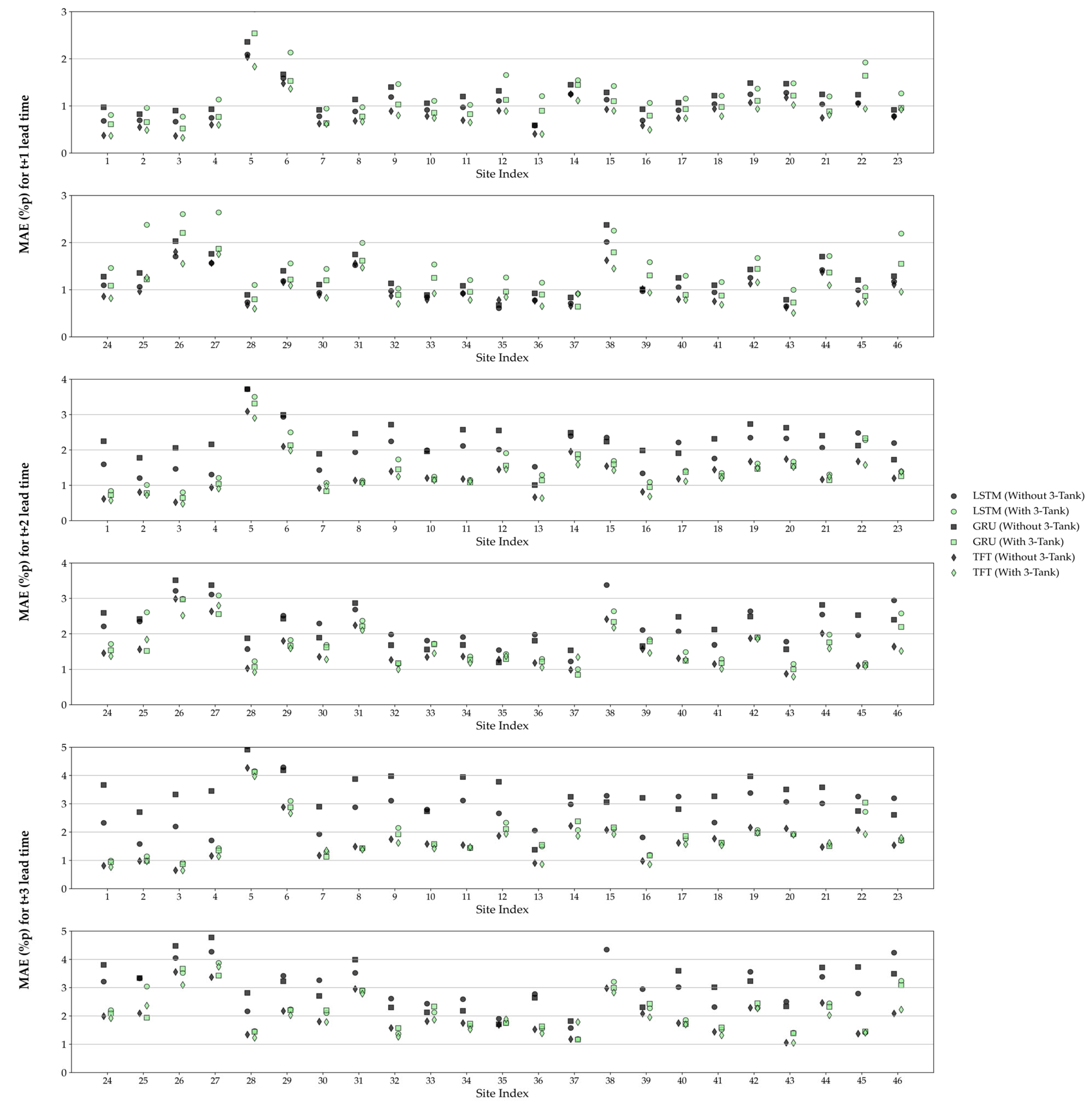
Figure 11 presents the MAEs for 46 reservoirs across the three AI models with inflow and outflow variables for 1-day, 2-day, and 3-day-ahead forecasts. For the 1-day-ahead forecast, the error either remained similar or slightly increased for some reservoirs, but a decrease in error was observed in the majority of reservoirs. Notably, in the 2-day and 3-day-ahead reservoir water level forecasts, the accuracy with the application of with inflow and outflow variables was significantly superior compared to when they were not applied, and the errors of the LSTM and GRU models with the additional variables were meaningfully smaller than their counterparts without. Comparing the results by model, TFT model exhibited smaller errors than the LSTM and GRU models for most reservoirs, when the inflow and outflow variables were applied or not.
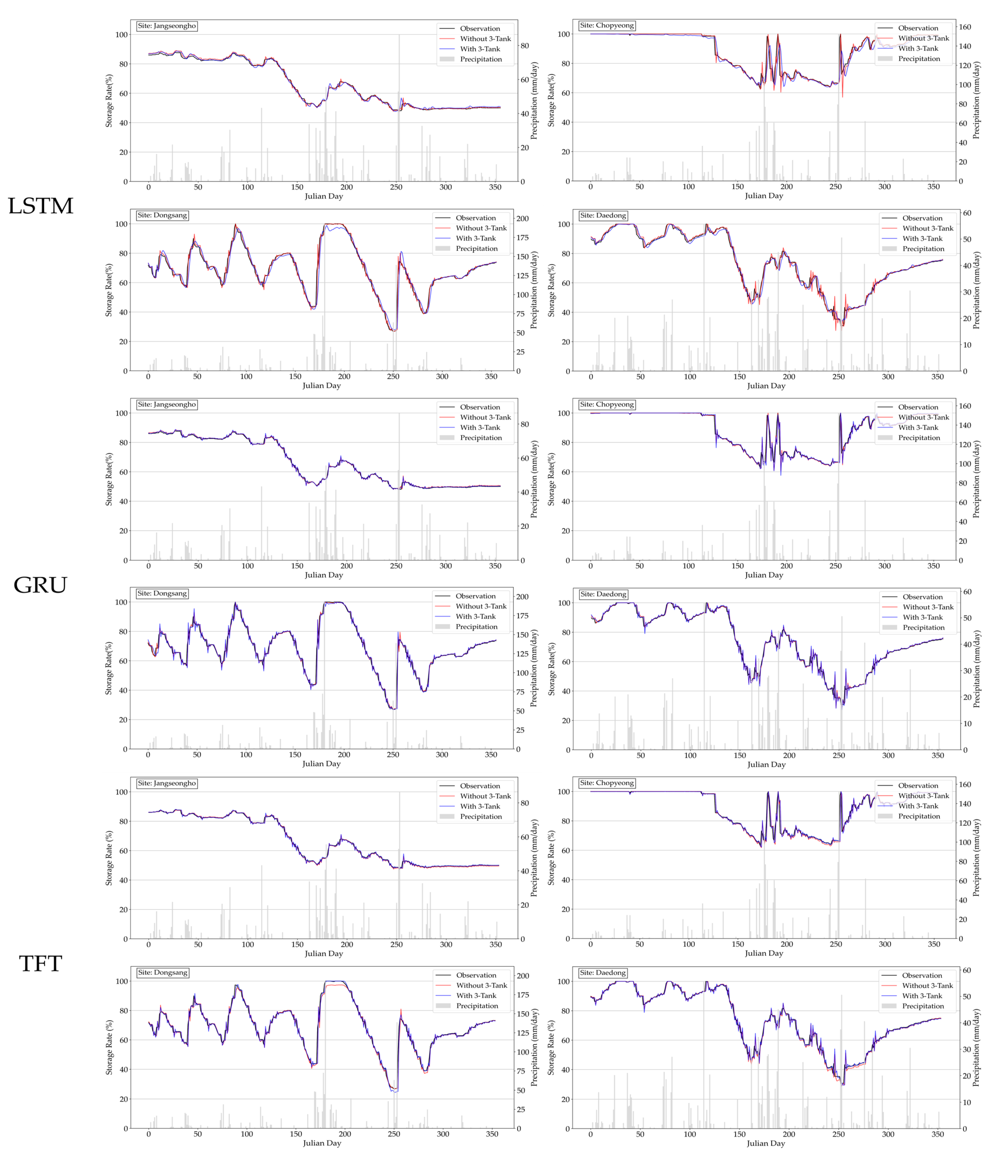
Figure 12 displays a comparison graph of the 1-day-ahead reservoir water level forecasts for the Jangseong, Chopyeong, Dongsan, and Daedong Reservoirs using the test dataset. The black line represents the observed water level, the red line is the predicted value from the without 3TM, the blue line is the predicted value from the with 3TM, and the gray bars indicate the daily cumulative rainfall. For Jangseong Reservoir, which has a large effective storage capacity, all model configurations performed the prediction with high accuracy, despite the greater fluctuation range in the water level compared to the Chopyeong, Dongsan, and Daedong reservoirs. Conversely, for Chopyeong Reservoir, which has a smaller effective storage capacity than Jangseong, the LSTM and GRU models without 3TM showed large errors in segments where the water level changed significantly. However, the LSTM and GRU models with 3TM predicted these segments with a smaller error compared to the without 3TM counterparts. The TFT model, both with and without 3TM, predicted the rapidly changing water levels with a small error. Similarly, for Daedong Reservoir, which is among the smaller reservoirs in terms of effective storage capacity, the LSTM and GRU models without 3TM had large errors in areas of significant water level change. Nevertheless, the LSTM and GRU models with 3TM achieved the prediction with a smaller error, and the TFT model performed the prediction with a small error in both with and without 3TM (inflow and outflow variables).

3.2.2. Comparison of AI Models for Flood Control Period

Reservoir waters can be released during flood control periods. Table 9 compares the averaged prediction statistics for 46 reservoirs under both with and without 3TM conditions for 1-day, 2-day, and 3-day-ahead forecasts during the flood control period. The accuracy of reservoir water level forecasting typically decreases during the flood control period due to the concentration of heavy rainfall and the resultant large fluctuations in water levels. However, accuracy can be improved by incorporating inflow and outflow variables into the water level prediction. For the 1-day-ahead forecast, the MAEs for the LSTM, GRU, and TFT models without 3TM were 2.314%p, 2.394%p, and 2.346%p, respectively. In contrast, the MAEs for the models with 3TM were 2.055%p, 2.134%p, and 2.042%p, demonstrating an improvement in prediction accuracy of approximately 0.3%p when the 3TM inflow and outflow variables were applied. Furthermore, in the 2-day and 3-day-ahead forecasts, the MAEs for the models with 3TM were also improved by approximately 0.5%p and 0.6%p, respectively. Comparing the prediction accuracy between the TFT and RNN models, the TFT model was superior by a maximum of 0.4%p in terms of MAEs during non-flood control periods. However, during the flood control period, the MAE of the TFT model with 3TM was nearly identical to the LSTM and GRU models with 3TM, with a difference of only 0.01%p for the 1-day-ahead forecast and 0.1%p for the 2-day and 3-day-ahead forecasts. This can be interpreted as the RNN models having better learned the complex features amidst the rapidly changing meteorological conditions of the flood control period. Overall, the models with 3TM inflow and outflow variables demonstrated higher accuracy in forecasting reservoir water levels compared to those without 3TM, even during the flood control period.

3.3. BMA Ensemble

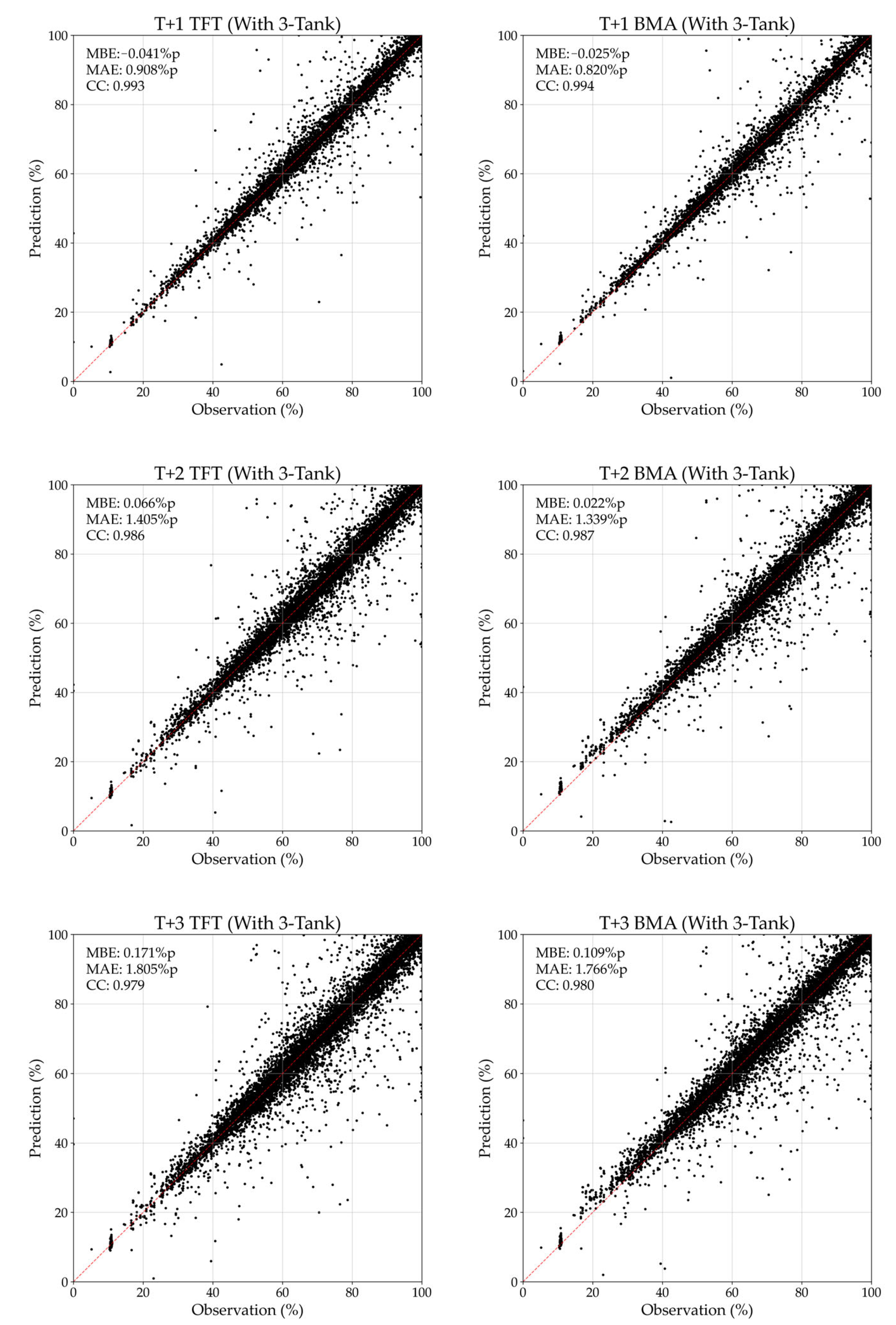
Although the TFT model exhibited the best performance in almost all cases, an ensemble of the LSTM, GRU, and TFT models using the BMA technique can potentially yield even better performance than the standalone TFT model. Table 10 compares the statistics of the TFT single model (which had the smallest error among single models) with the statistics of the ensemble model applying BMA to the prediction results of the LSTM, GRU, and TFT models with 3TM inflow and outflow variables. The MAE of the BMA for the 1-day-ahead forecast was 0.820%p, which is smaller than the 0.908%p of the TFT model. For the 2-day and 3-day-ahead forecasts, the BMA MAEs were 1.339%p and 1.766%p, respectively, which were also smaller than the 1.405%p and 1.805%p errors shown by the TFT model.
Figure 13 presents scatter plots comparing the predicted and observed reservoir water levels for all target reservoirs in the test dataset for 1-day, 2-day, and 3-day-ahead forecasts. The red dashed line represents the 1:1 line, and almost all cases align with the 1:1 line. A few points on the scatter plot deviate from the 1:1 line, which can be categorized into two cases. The cases where the reservoir water level was overpredicted compared to the observed value typically occurred when the models failed to accurately predict the sudden drop in water level due to reservoir release (discharge). Conversely, the cases where the reservoir water level was underpredicted compared to the observed value generally represent the models failing to accurately predict the rapid increase in water level caused by concentrated heavy rainfall. When the reservoir water level fluctuates widely due to natural or artificial factors, single models may yield inaccurate predictions, and the BMA ensemble of these results may also not show an effective improvement in accuracy. Nevertheless, both the TFT and BMA with the 3TM inflow and outflow variables demonstrate excellent predictive performance in the majority of cases, as evidenced by the points clustering near the 1:1 line. Although the scatter plots show no visually striking difference between the TFT and BMA ensemble, the improvement in the MAE and correlation coefficient metrics indicates that BMA ensemble achieved a higher prediction accuracy compared to the single model.
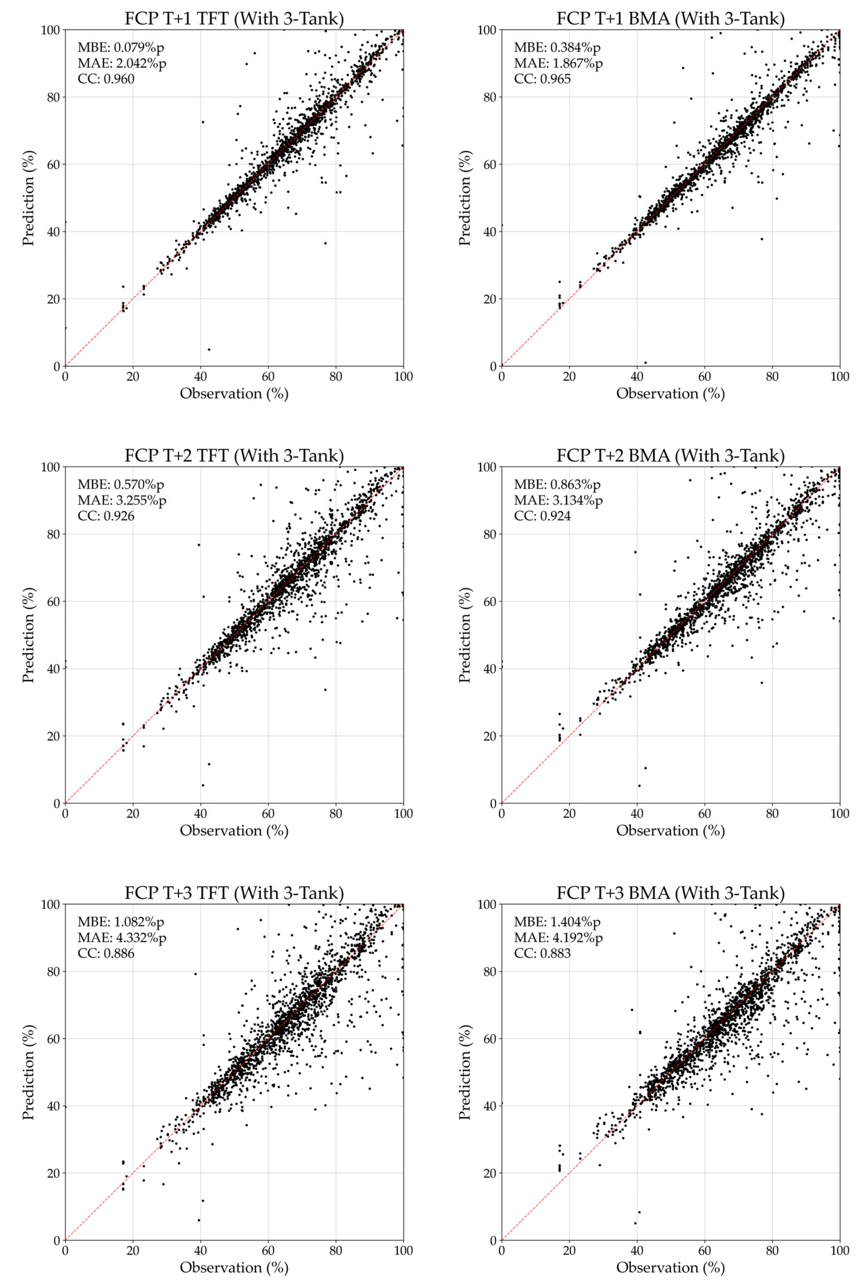
In Table 11, we compare the statistics of the Flood Control Regulator using the TFT and BMA ensembles with 3TM. The MAE for the 1-day-ahead prediction of the BMA ensemble was 1.867%p, which is an error 0.175%p smaller than the 2.042%p of the TFT, which showed the best prediction performance among the single models. For the 2-day-ahead and 3-day-ahead predictions, the MAEs of the BMA ensemble were 3.134%p and 4.192%p, which were also smaller than the 3.255%p and 4.322%p of the TFT. Although the correlation coefficients for the 2-day-ahead and 3-day-ahead predictions for the TFT and BMA ensemble are similar, the improvement in absolute error indicates that the BMA ensembles also provided superior predictions compared to the single model for the flood control periods.
In Figure 14, we present scatter plots comparing the predicted values against the observed values for the flood control periods of all targeted reservoirs, for 1-day, 2-day, and 3-day-ahead forecasts. Both the TFT and BMA ensembles generally provide predictions that are close to the observed values while a few points with significant changes in reservoir water levels deviate from the 1:1 line. As the forecast horizon increases for both models, the scatter plot points tend to move further away from the 1:1 line. However, it can be observed that for the BMA ensemble, the points remain distributed slightly closer to the 1:1 line compared to the TFT model, even with an increasing forecast horizon. Furthermore, the BMA ensemble demonstrated superior performance with an approximately 0.2%p lower MAE compared to the TFT model.
Figure 15 shows a time series plot comparing the 1-day-ahead prediction results of the BMA ensemble and single models. The black line represents the observed reservoir water level, the yellow line indicates the predicted values from the BMA ensemble, while the red, green, and blue dashed lines correspond to the predictions of the LSTM, GRU, and TFT single models, respectively. For the Jangseong Reservoir, which has the largest effective storage capacity, both the single models and the BMA ensemble predicted the water level with a small error. In contrast, at the Chopyeong Reservoir, which has a smaller effective storage capacity, the TFT model showed an overestimation when the water level changed drastically. However, the BMA ensemble provided predictions with only a small error. For the Dongsang Reservoir, where the increase in water level was relatively gradual, both the single models and the BMA ensemble made predictions with minimal error. Similarly, at the Daedong Reservoir, which also has a small effective storage capacity, the TFT model somewhat overestimated the water level during periods of large changes, whereas the BMA model maintained a small prediction error.

3.4. Feature Importance

To analyze the contribution of each input feature to the reservoir water level prediction, the input feature importance was derived based on the attention mechanism of the TFT model (Table 12). The past reservoir water level was found to be the most important variable for predicting the water level, with a contribution of 43.42%, which can be attributed to the temporal continuity between the water level at time t and t + 1. Following the historical water level, the inflow and outflow from 3TM were the next most important variables, with importance values of 11.24% and 10.78%, respectively. The inclusion of these variables consistently improved model accuracy under all conditions. Meteorological data, including precipitation and evaporation, showed importance values of 9.50% and 7.84%, respectively, demonstrating the significance of incorporating external meteorological information for accurate reservoir water level prediction. Temporal trend represented by Relative Time Index, which indicates the relative temporal position with respect to the prediction time, allows the TFT model to react differently depending on the time position, thereby enhancing prediction accuracy. The Julian day transformed in a cosine format can be interpreted as the model learning the cyclical pattern of water level fluctuations in agricultural reservoirs that occur on an annual basis.

4. Discussion

In this study, we propose a framework for reservoir water level prediction that integrates time-series AI models with 3TM. The 3TM rainfall–runoff model derives inflow and outflow variables which are then used as input features for the AI models. Final predictions are refined using a BMA ensemble for advanced accuracy. The Discussion section interprets the effect of BMA results, explores the significance of incorporating the simulated inflow and outflow variables from 3TM, and addresses the study’s limitations.

4.1. Effect of BMA Ensemble

Across the entire study period, the TFT model showed a best performance among the three models (LSTM, GRU, and TFT) for predictions from 1, 2, and 3 days ahead. Although LSTM and GRU are less accurate than TFT, the LSTM and GRU also contributed to the accuracy improvement via the BMA ensemble, then produced better performance than the top 1 model TFT. BMA is a powerful ensemble technique for improving the accuracy of machine learning models, particularly due its capability of the integration of model uncertainty. BMA assigns weights based on the posterior probability of each candidate model. This means models that performed better on past data are given greater weight, thus increasing prediction accuracy and resolving the uncertainty associated with model selection. In addition, BMA can prevent overfitting by combining the predictions of multiple models, thereby enhancing the generalization performance on new data. Owing to these characteristics, BMA has been studied as a solution for the hydrological and meteorological time-series prediction such as streamflow, water level, evapotranspiration and soil moisture, where uncertainty is high and complex nonlinear relationships are prevalent. As shown in the comparative charts for the Chopyeong and Daedong Reservoirs in Figure 15, the TFT model, although it is the top 1 model, overpredicted the reservoir water level during periods of large changes. However, with the help of blending of LSTM and GRU, the BMA ensemble model demonstrated superior predictive performance compared to the single models across all periods. In addition to TFT, the other Transformer time-series models such as Frequency Enhanced Decomposed Transformer (FEDformer), and Patch Time-Series Transformer (PatchTST) can also be included in the BMA ensemble. Moreover, a meta-learner through model stacking will be useful because it allows the model to learn the optimal way to combine predictions from diverse base models, leveraging the strengths of each to improve overall accuracy and generalization.

4.2. Roles of Inflow and Outflow Variables

As shown in the previous results, incorporating the simulated inflow and outflow variables into the reservoir water level prediction model improved accuracy under most conditions, with a particularly notable enhancement during the flood control period. When modeling a reservoir storage, variables such as precipitation, evaporation, inflow, and outflow must be considered. If inflow, a key variable for rising water levels, is not considered, there is a degree of uncertainty in the prediction equal to the amount of unaccounted for inflow. Similarly, if outflow, a variable critical for declining water levels, is not considered, it introduces a corresponding level of uncertainty. Therefore, simulating and utilizing the inflow and outflow of a reservoir for prediction effectively reduces this modeling uncertainty and improves accuracy. Moreover, while a rise in reservoir water level is determined by natural causes such as precipitation and inflow from surrounding watersheds, a decrease in water level due to outflow is an artificial factor governed by reservoir operation rules. By simulating this artificial variable using reservoir operation rules and incorporating it into the water level prediction model, we can enable the model to learn these rules, leading to an expected improvement in prediction accuracy.

4.3. Limitations and Future Work

While this study proposes a framework for highly accurate prediction of agricultural reservoir water levels, it has a few limitations. This research was conducted on the top 46 agricultural reservoirs in South Korea based on effective storage capacity. These reservoirs have effective storage capacities ranging from a minimum of 7,001,000 m3 to a maximum of 107,000,000 m3, with an average of approximately 21,000,000 m3. While the framework demonstrated high accuracy for these large-scale reservoirs for predictions from 1, 2, and 3 days ahead, its performance might not be as high for smaller reservoirs. Small reservoirs are susceptible to rapid filling during the rainy season compared to large reservoirs, causing significant water storage fluctuations that may pose a challenge to accurate prediction with daily interval forecasts [72,73]. Hence, we have conducted experiments for a small reservoir which was not included the in the modeling process. Cheontae Reservoir has very small effective storage capacity (1,290,000 m3), only 6% of the average capacity of the 46 reservoirs. However, the MAEs for 1, 2, and 3 days ahead prediction were 1.127%p, 1.442%p, and 1.759%p, respectively. This is very similar result 0.820%p, 1.339%p, and 1.766%p for the blind test of 2024. Future work could focus on improving prediction accuracy by validating both hourly and daily prediction performance for small reservoirs where hourly storage data are available.
Additionally, the meteorological data used as input for the AI prediction and 3TM was sourced from the weather station closest to each reservoir. Due to South Korea’s mountainous terrain and complex geographical characteristics, the uncertainty of meteorological data can increase if complex topography exists between the reservoir and the weather station. While many of the reservoirs in this study are in the western plains of South Korea, some are located in mountainous regions. Future studies should address this issue by exploring the integration of higher-resolution meteorological datasets or the deployment of localized weather monitoring stations to improve the spatial representativeness of meteorological variables and reduce data uncertainty.
Finally, while reservoir operation rules were used to simulate inflow and outflow for the 3TM, not all reservoirs are operated strictly according to these rules every year. This study assumes that reservoirs are managed in line with the rules during the cultivation and flood control periods. However, a manager’s judgment can intervene depending on the specific situation of each reservoir, which introduces a degree of uncertainty when utilizing the reservoir operation rules. Future work will focus on addressing these limitations.

5. Conclusions

In this study, we propose a framework for predicting agricultural reservoir water levels with high accuracy, even during rapidly changing weather conditions. A key finding is that for reservoirs lacking inflow and outflow data, we can accurately simulate these two variables using only reservoir water level and meteorological station data, and by incorporating them into the prediction model, we achieve higher accuracy than conventional methods. For 1-day-ahead predictions, the MAEs for LSTM, GRU, and TFT were 1.116%p, 1.025%p, and 1.047%p, respectively, without the additional variables. However, with the added variables, the MAEs significantly decreased to 0.930%p, 0.977%p, and 0.908%p. For 3-day-ahead predictions, the TFT model’s MAE was in the 1%p range, while LSTM and GRU’s were in the 2%p range, demonstrating a significant improvement in TFT’s accuracy for longer-term predictions. Specifically, during the flood control period, when heavy rainfall is concentrated, the MAEs for 1-day-ahead predictions were 2.314%p, 2.374%p, and 2.346%p under the “Without 3TM” condition. This error was reduced to 2.055%p, 2.134%p, and 2.042%p, respectively, under the “With 3TM” condition. The ensemble model, which applies BMA to the single model predictions, showed superior accuracy with MAEs of 0.820%p, 1.339%p, and 1.766%p for 1-day, 2-day, and 3-day-ahead predictions. This performance is an improvement over the most accurate single model, TFT, which had MAEs of 0.908%p, 1.405%p, and 1.805%p. The ensemble model also demonstrated more stable predictions during the flood control period compared to the single models. The proposed framework is expected to enable highly accurate water level predictions for reservoirs that do not provide inflow and outflow data. By building a robust prediction model that can withstand rapidly changing weather conditions, it will be possible to establish proactive reservoir operation plans, prevent flood damage to facilities and prevent downstream areas from being affected by flood overflows. Furthermore, it will facilitate the smooth operation of agricultural reservoirs by enabling the appropriate discharge of irrigation water to downstream agricultural lands.

Author Contributions

Conceptualization, J.P., J.S.-u.J., M.C., T.K., J.C. and Y.L.; methodology, J.P., J.S.-u.J., M.C., T.K., J.C. and Y.L.; data curation, J.P.; formal analysis, J.P.; writing—original draft preparation, J.P.; writing—review and editing, J.S.-u.J., M.C., T.K., J.C. and Y.L.; project administration, Y.L. All authors have read and agreed to the published version of the manuscript.

Funding

This work is supported by the Korea Agency for Infrastructure Technology Advancement (KAIA) grant funded by the Ministry of Land, Infrastructure and Transport (Grant RS-2022-00155763). This research was supported by a grant (2021-MOIS37-002) of Intelligent Technology Development Program on Disaster Response and Emergency Management funded by Ministry of Interior and Safety (MOIS, Korea).

Data Availability Statement

The raw data supporting the conclusions of this article will be made available by the authors on request.

Conflicts of Interest

The authors declare no conflicts of interest.

Appendix A. Reservoir Operation Rule

  • In crop-growing periods, reservoir water is released only to provide the irrigation water supply. The crop-growing period consists of the interruption and drawdown periods.
  • In the interruption period, irrigation water supply stops even when it is the middle of the crop-growing period (zero-outflow period).
  • In the drawdown periods, reservoir water is released through the drainage spillway to supply irrigation water for the downstream areas.
  • When the reservoir level decreases below the dead level, irrigation water supply stops (zero-outflow period).
  • In the flood control period, the principal spillway release is made to accommodate space for excess water inflow to precent the reservoir water level from exceeding the flood-limited water level.
  • When the irrigation periods overlap with the flood control periods, priority is given to flood control in reservoir operations; thus, irrigation water supply is released only when the reservoir water level drops below the flood-limited water level to protect downstream areas from flooding.
  • In the non-flood control and non-crop-growing periods, the reservoir collects inflow from its upstream drainage areas until its water level reaches the normal pool water level for water supply during the next growing period.
  • In the non-flood control period, when reservoir water level exceeds the normal pool water level, the surcharge water is discharged through the normal pool spillway.

References

  1. Kim, W.; Choi, S.; Kang, S.; Woo, S. Assessment of Future Water Security under Climate Change: Practical Water Allocation Scenarios in a Drought-Prone Watershed in South Korea. Water 2024, 16, 2933. [Google Scholar] [CrossRef]
  2. Ciampittiello, M.; Marchetto, A.; Boggero, A. Water Resources Management under Climate Change: A Review. Sustainability 2024, 16, 3590. [Google Scholar] [CrossRef]
  3. Bae, H.; Ji, H.; Lim, Y.; Ryu, Y.; Kim, M.; Kim, B. Characteristics of drought propagation in South Korea: Relationship between meteorological, agricultural, and hydrological droughts. Nat. Hazards 2019, 99, 1–16. [Google Scholar] [CrossRef]
  4. Noh, S.; Lee, G.; Kim, B.; Jo, J.; Woo, D. Climate change impact analysis on water supply reliability and flood risk using combined rainfall-runoff and reservoir operation modeling: Hapcheon-Dam catchment case. J. Korea Water Resour. Assoc. 2023, 56, 765–774. [Google Scholar] [CrossRef]
  5. Yi, S.; Yi, J. Reservoir-based flood forecasting and warning: Deep learning versus machine learning. Appl. Water Sci. 2024, 14, 237. [Google Scholar] [CrossRef]
  6. Cho, G.; Ahmad, M.J.; Choi, K. Water Supply Reliability of Agricultural Reservoirs under Varying Climate and Rice Farming Practices. Water 2021, 13, 2988. [Google Scholar] [CrossRef]
  7. Song, J.; Kang, M.; Song, I.; Jun, S. Water Balance in Irrigation Reservoirs Considering Flood Control and Irrigation Efficiency Variation. J. Irrig. Drain. Eng. 2016, 142, 04016003. [Google Scholar] [CrossRef]
  8. Wurbs, R.A. Reservoir-system simulation and optimization models. J. Water Resour. Plan. Manag. 1993, 119, 455–472. [Google Scholar] [CrossRef]
  9. Bengtsson, L.; Malm, J. Using rainfall-runoff modeling to interpret lake level data. J. Paleolimnol. 1997, 18, 235–248. [Google Scholar] [CrossRef]
  10. Wagener, T.; Wheater, H.; Gupta, H.V. Rainfall-Runoff Modelling in Gauged and Ungauged Catchments; Imperial College Press: London, UK, 2004; pp. 119–183. ISBN 1-86094-466-3. [Google Scholar]
  11. Beven, K.J. Rainfall-Runoff Modelling: The Primer, 2nd ed.; Wiley-Blackwell Press: Oxford, UK, 2012; ISBN 978-0-470-71459-1. [Google Scholar]
  12. Arnold, J.G.; Srinivasan, R.; Muttiah, R.S.; Williams, J.R. Large area hydrologic modeling and assessment part I: Model development. J. Am. Water Resour. Assoc. 1998, 34, 73–89. [Google Scholar] [CrossRef]
  13. Beven, K. A manifesto for the equifinality thesis. J. Hydrol. 2006, 320, 18–36. [Google Scholar] [CrossRef]
  14. Singh, V.P.; Woolhiser, D.A. Mathematical modeling of watershed hydrology. J. Hydrol. Eng. 2002, 7, 270–292. [Google Scholar] [CrossRef]
  15. Gupta, H.V.; Wagener, T.; Liu, Y. Reconciling theory with observations: Elements of a diagnostic approach to model evaluation. Hydrol. Process. 2008, 22, 3802–3813. [Google Scholar] [CrossRef]
  16. Irvine, K.N.; Eberhardt, A.J. Multiplicative, Seasonal Arima Models for Lake Erie and Lake Ontario Water Levels1. J. Am. Water Resour. Assoc. 2007, 28, 385–396. [Google Scholar] [CrossRef]
  17. Das, M.; Ghosh, S.K.; Chowdary, V.M.; Saikrishnaveni, A.; Sharma, R.K. A Probabilistic Nonlinear Model for Forecasting Daily Water Level in Reservoir. Water Resour. Manag. 2016, 30, 3107–3122. [Google Scholar] [CrossRef]
  18. Ahn, T.; Lee, J.; Lee, J.; Yi, J.; Yoon, Y. A reservoir operation plan coupled with storage forecasting models in existing agricultural reservoir. J. Korea Water Resour. Assoc. 2004, 37, 77–86. [Google Scholar] [CrossRef]
  19. Kovvuri, A.R.; Uppalapati, P.J.; Bonthu, S.; Kandula, N.R. Water level forecasting in reservoirs using time series analysis–auto ARIMA model. In Proceedings of the International Conference on Cognitive Computing and Cyber Physical Systems (IC4S 2022), Ghaziabad, Indea, 24–26 November 2022; pp. 192–200. [Google Scholar]
  20. Khan, M.S.; Coulibaly, P. Application of support vector machine in lake water level prediction. J. Hydrol. Eng. 2006, 11, 199–205. [Google Scholar] [CrossRef]
  21. Khai, W.J.; Alraih, M.; Ahmed, A.N.; Fai, C.M.; El-Shafie, A.; El-Shafie, A. Daily forecasting of dam water levels using machine learning. Int. J. Civ. Eng. Technol. 2019, 10, 314–323. [Google Scholar] [CrossRef]
  22. Hipni, A.; El-shafie, A.; Najah, A.; Karim, O.A.; Hussain, A.; Mukhlisin, M. Daily Forecasting of Dam Water Levels: Comparing a Support Vector Machine (SVM) Model With Adaptive Neuro Fuzzy Inference System (ANFIS). Water Resour. Manag. 2013, 27, 3803–3823. [Google Scholar] [CrossRef]
  23. Chang, F.-J.; Chang, Y.-T. Adaptive neuro-fuzzy inference system for prediction of water level in reservoir. Adv. Water Resour. 2006, 29, 1–10. [Google Scholar] [CrossRef]
  24. Valizadeh, N. Daily water level forecasting using adaptive neuro-fuzzy interface system with different scenarios: Klang Gate, Malaysia. Int. J. Phys. Sci. 2011, 6, 7379–7389. [Google Scholar] [CrossRef]
  25. Shrestha, B.P.; Duckstein, L.; Stakhiv, E.Z. Fuzzy rule-based modeling of reservoir operation. J. Water Resour. Plan. Manag. 1996, 122, 262–269. [Google Scholar] [CrossRef]
  26. Unes, F. Prediction of dam reservoir volume fluctuations using adaptive neuro fuzzy approach. Eur. J. Eng. Nat. Sci. 2017, 2, 144–148. [Google Scholar]
  27. Zhang, Y.; Dai, X.; Wan, R.; Yang, G.; Li, B. Comparison of random forests and other statistical methods for the prediction of lake water level: A case study of the Poyang Lake in China. Hydrol. Res. 2016, 47, 69–83. [Google Scholar] [CrossRef]
  28. Ouma, Y.O.; Moalafhi, D.B.; Anderson, G.; Nkwae, B.; Odirile, P.; Parida, B.P.; Qi, J. Dam Water Level Prediction Using Vector AutoRegression, Random Forest Regression and MLP-ANN Models Based on Land-Use and Climate Factors. Sustainability 2022, 14, 14934. [Google Scholar] [CrossRef]
  29. Anindita, A.P.; Laksono, P.; Nugraha, I.G.B.B. Dam water level prediction system utilizing Artificial Neural Network Back Propagation: Case study: Ciliwung watershed, Katulampa Dam. In Proceedings of the 2016 International Conference on ICT For Smart Society (ICISS 2016), Surabaya, Indonesia, 20–21 July 2016; pp. 16–21. [Google Scholar]
  30. Nwobi-Okoye, C.C.; Igboanugo, A.C. Predicting water levels at Kainji Dam using artificial neural networks. Niger. J. Technol. 2013, 32, 129–136. [Google Scholar]
  31. Seo, Y.; Choi, E.; Yeo, W. Reservoir Water Level Forecasting Using Machine Learning Models. J. Korean Soc. Agric. Eng. 2017, 59, 97–110. [Google Scholar] [CrossRef]
  32. Li, K.; Wan, D.; Zhu, Y.; Yao, C.; Yu, Y.; Si, C.; Ruan, X. The applicability of ASCS_LSTM_ATT model for water level prediction in small- and medium-sized basins in China. J. Hydroinform. 2020, 22, 1693–1717. [Google Scholar] [CrossRef]
  33. Nie, Q.; Wan, D.; Wang, R. CNN-BiLSTM water level prediction method with attention mechanism. J. Phys. Conf. Ser. 2021, 2078, 12–32. [Google Scholar] [CrossRef]
  34. Kimura, N.; Yoshinaga, I.; Sekijima, K.; Azechi, I.; Baba, D. Convolutional Neural Network Coupled with a Transfer-Learning Approach for Time-Series Flood Predictions. Water 2019, 12, 96. [Google Scholar] [CrossRef]
  35. Kusudo, T.; Yamamoto, A.; Kimura, M.; Matsuno, Y. Development and Assessment of Water-Level Prediction Models for Small Reservoirs Using a Deep Learning Algorithm. Water 2021, 14, 55. [Google Scholar] [CrossRef]
  36. Zhang, Y.; Zhou, Z.; Van Thé, J.G.; Yang, S.X.; Gharabaghi, B. Flood Forecasting Using Hybrid LSTM and GRU Models with Lag Time Preprocessing. Water 2023, 15, 3982. [Google Scholar] [CrossRef]
  37. Joh, S.; Lee, Y. Prediction of water storage rate for agricultural reservoirs using univariate and multivariate LSTM models. Korean J. Remote Sens. 2023, 39, 1125–1134. [Google Scholar] [CrossRef]
  38. Xie, M.; Shan, K.; Zeng, S.; Wang, L.; Gong, Z.; Wu, X.; Yang, B.; Shang, M. Combined Physical Process and Deep Learning for Daily Water Level Simulations Across Multiple Sites in the Three Gorges Reservoir, China. Water 2023, 15, 3191. [Google Scholar] [CrossRef]
  39. Li, H.; Zhang, L.; Zhang, Y.; Yao, Y.; Wang, R.; Dai, Y. Water-Level Prediction Analysis for the Three Gorges Reservoir Area Based on a Hybrid Model of LSTM and Its Variants. Water 2024, 16, 1227. [Google Scholar] [CrossRef]
  40. Duan, Q.; Ajami, N.K.; Gao, X.; Sorooshian, S. Multi-model ensemble hydrologic prediction using Bayesian model averaging. Adv. Water Resour. 2007, 30, 1371–1386. [Google Scholar] [CrossRef]
  41. Song, J.; Her, Y.; Kang, M. Estimating Reservoir Inflow and Outflow from Water Level Observations Using Expert Knowledge: Dealing with an Ill-Posed Water Balance Equation in Reservoir Management. Water Resour. Res. 2022, 58, e2020WR028183. [Google Scholar] [CrossRef]
  42. Available online: https://www.data.go.kr/data/15099919/openapi.do (accessed on 16 October 2025).
  43. Available online: https://www.data.go.kr/data/15099051/openapi.do (accessed on 16 October 2025).
  44. Bengio, S.; Vinyals, O.; Jaitly, N.; Shazeer, N. Scheduled sampling for sequence prediction with recurrent neural networks. In Advances in Neural Information Processing Systems; Curran Associates, Inc.: Red Hook, NY, USA, 2015; Volume 28. [Google Scholar]
  45. Lim, B.; Zohren, S. Time-series forecasting with deep learning: A survey. Philos. Trans. R. Soc. A Math. Phys. Eng. Sci. 2021, 379, 20200209. [Google Scholar] [CrossRef]
  46. Lim, B.; Arık, S.Ö.; Loeff, N.; Pfister, T. Temporal Fusion Transformers for interpretable multi-horizon time series forecasting. Int. J. Forecast. 2021, 37, 1748–1764. [Google Scholar] [CrossRef]
  47. Kim, M.; Lee, W.K.; Son, Y.; Yoo, S.; Choi, G.M.; Chung, D.J. Assessing the impacts of topographic and climatic factors on radial growth of major forest forming tree species of South Korea. For. Ecol. Manag. 2017, 404, 269–279. [Google Scholar] [CrossRef]
  48. Wook, P.; Jong, J. Reservoir water monitoring system with automatic level meter. Korean Natl. Comm. Irrig. Drain. 2005, 12, 60–68. [Google Scholar]
  49. Available online: https://www.data.go.kr/data/15059093/openapi.do (accessed on 16 October 2025).
  50. Fu, G.; Liu, C.; Chen, S.; Hong, J. Investigating the conversion coefficients for free water surface evaporation of different evaporation pans. Hydrol. Process. 2004, 18, 2247–2262. [Google Scholar] [CrossRef]
  51. Habets, F.; Molenat, J.; Carluer, N.; Douez, O.; Leenhardt, D. The cumulative impacts of small reservoirs on hydrology: A review. Sci. Total Environ. 2018, 643, 850–867. [Google Scholar] [CrossRef] [PubMed]
  52. Song, J.; Her, Y.; Park, J.; Kang, M. Exploring parsimonious daily rainfall-runoff model structure using the hyperbolic tangent function and Tank model. J. Hydrol. 2019, 574, 574–587. [Google Scholar] [CrossRef]
  53. Vedula, S.; Kumar, D.N. An Integrated Model for Optimal Reservoir Operation for Irrigation of Multiple Crops. Water Resour. Res. 1996, 32, 1101–1108. [Google Scholar] [CrossRef]
  54. Dang, T.D.; Chowdhury, A.F.M.K.; Galelli, S. On the representation of water reservoir storage and operations in large-scale hydrological models: Implications on model parameterization and climate change impact assessments. Hydrol. Earth Syst. Sci. 2020, 24, 397–416. [Google Scholar] [CrossRef]
  55. Dessie, M.; Verhoest, N.E.C.; Pauwels, V.R.N.; Adgo, E.; Deckers, J.; Poesen, J.; Nyssen, J. Water balance of a lake with floodplain buffering: Lake Tana, Blue Nile Basin, Ethiopia. J. Hydrol. 2015, 522, 174–186. [Google Scholar] [CrossRef]
  56. Chen, S.-K.; Chen, R.-S.; Yang, T.-Y. Application of a tank model to assess the flood-control function of a terraced paddy field. Hydrol. Sci. J. 2014, 59, 1020–1031. [Google Scholar] [CrossRef]
  57. Fumikazu, N.; Toshisuke, M.; Yoshio, H.; Hiroshi, T.; Kimihito, N. Evaluation of water resources by snow storage using water balance and tank model method in the Tedori River basin of Japan. Paddy Water Environ. 2011, 11, 113–121. [Google Scholar] [CrossRef]
  58. Yokoo, Y.; Kazama, S.; Sawamoto, M.; Nishimura, H. Regionalization of lumped water balance model parameters based on multiple regression. J. Hydrol. 2001, 264, 209–222. [Google Scholar] [CrossRef]
  59. Atkinson, S.E.; Woods, R.A.; Sivapalan, M. Climate and landscape controls on water balance model complexity over changing timescales. Water Resour. Res. 2002, 38, 50-1–50-17. [Google Scholar] [CrossRef]
  60. Deb, K.; Pratap, A.; Agarwal, S.; Meyarivan, T.A.M.T. A fast and elitist multiobjective genetic algorithm: NSGA-II. IEEE Trans. Evol. Comput. 2002, 6, 182–197. [Google Scholar] [CrossRef]
  61. Krause, P.; Boyle, D.P.; Bäse, F. Comparison of different efficiency criteria for hydrological model assessment. Adv. Geosci. 2005, 5, 89–97. [Google Scholar] [CrossRef]
  62. Shin, M.J.; Kim, C.S. Assessment of the suitability of rainfall–runoff models by coupling performance statistics and sensitivity analysis. Hydrol. Res. 2017, 48, 1192–1213. [Google Scholar] [CrossRef]
  63. Moriasi, D.N.; Arnold, J.G.; Van Liew, M.W.; Bingner, R.L.; Harmel, R.D.; Veith, T.L. Model evaluation guidelines for systematic quantification of accuracy in watershed simulations. Trans. ASABE 2007, 50, 885–900. [Google Scholar] [CrossRef]
  64. Hochreiter, S.; Bengio, Y.; Frasconi, P.; Schmidhuber, J. Gradient flow in recurrent nets: The difficulty of learning long-term dependencies. In A Field Guide to Dynamical Recurrent Neural Networks; IEEE Press: Piscataway, NJ, USA, 2001; pp. 237–243. [Google Scholar] [CrossRef]
  65. Bengio, Y.; Simard, P.; Frasconi, P. Learning long-term dependencies with gradient descent is difficult. IEEE Trans. Neural Netw. 1994, 5, 157–166. [Google Scholar] [CrossRef] [PubMed]
  66. Hochreiter, S.; Schmidhuber, J. Long short-term memory. Neural Comput. 1997, 9, 1735–1780. [Google Scholar] [CrossRef]
  67. Cho, K.; Van Merriënboer, B.; Gulcehre, C.; Bahdanau, D.; Bougares, F.; Schwenk, H.; Bengio, Y. Learning phrase representations using RNN encoder-decoder for statistical machine translation. arXiv 2014. [Google Scholar] [CrossRef]
  68. Yin, W.; Kann, K.; Yu, M.; Schütze, H. Comparative study of CNN and RNN for natural language processing. arXiv 2017. [Google Scholar] [CrossRef]
  69. Chung, J.; Gulcehre, C.; Cho, K.; Bengio, Y. Empirical evaluation of gated recurrent neural networks on sequence modeling. arXiv 2014. [Google Scholar] [CrossRef]
  70. Vrugt, J.A.; Robinson, B.A. Treatment of uncertainty using ensemble methods: Comparison of sequential data assimilation and Bayesian model averaging. Water Resour. Res. 2007, 43, W01411. [Google Scholar] [CrossRef]
  71. Raftery, A.E.; Gneiting, T.; Balabdaoui, F.; Polakowski, M. Using Bayesian model averaging to calibrate forecast ensembles. Mon. Weather Rev. 2005, 133, 1155–1174. [Google Scholar] [CrossRef]
  72. Kumar Biswas, N.; Hossain, F. A Multidecadal Analysis of reservoir storage change in developing regions. J. Hydrometeorol. 2022, 23, 71–85. [Google Scholar] [CrossRef]
  73. Bonnema, M.; David, C.H.; Frasson, R.P.D.M.; Oaida, C.; Yun, S.H. The global surface area variations of lakes and reservoirs as seen from satellite remote sensing. Geophys. Res. Lett. 2022, 49, e2022GL098987. [Google Scholar] [CrossRef]
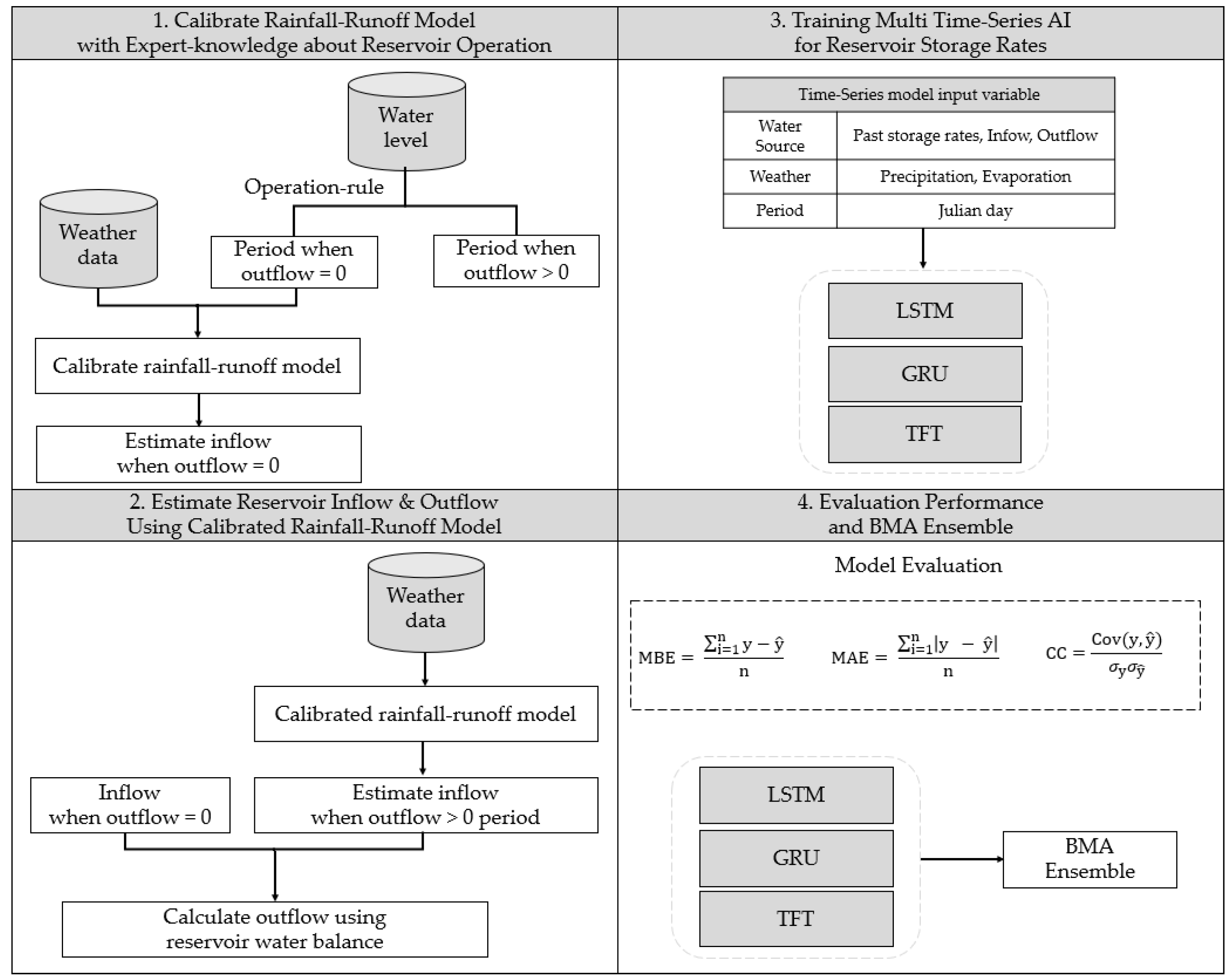
Figure 1. Overall workflow of the time-series AI for daily storage rates with operation rule-based rainfall–runoff process and BMA ensemble.
Water 17 03296 g001
Figure 2. Geographic locations of top 46 reservoirs by effective water storage used in this study.
Water 17 03296 g002
Figure 3. Functional roles of emergency, principal, and drainage spillways in relation to reservoir water levels.
Water 17 03296 g003
Figure 4. Conceptual diagram of Three-Tank Model (3TM) for simulating hydrological response to precipitation and evapotranspiration.
Water 17 03296 g004
Figure 5. Structure of LSTM and GRU units in the RNN-based time series model for reservoir storage rates prediction [67].
Water 17 03296 g005
Figure 6. Structure of the Temporal Fusion Transformer (TFT) model.
Water 17 03296 g006
Figure 7. Seasonal variation in storage rates in agricultural reservoir based on operation rules [41].
Water 17 03296 g007
Figure 8. Seasonal variations in storage rate and precipitation of Idong Reservoir in 2024 (flood control period in red line).
Water 17 03296 g008
Figure 9. Monthly cumulative precipitation, mean evaporation, and mean temperature, averaged across the 46 study reservoirs, based on data obtained from the nearest ASOS stations.
Water 17 03296 g009
Figure 10. Temporal uncertainty ranges of reservoir inflow estimates and corresponding observations for Jangseongho, Chopyeong, Dongsang, and Daedong Reservoirs, 2014–2024.
Water 17 03296 g010
Figure 11. Comparison of mean absolute errors (MAEs) of LSTM, GRU, and TFT models for the lead times t + 1, t + 2, and t + 3.
Water 17 03296 g011
Figure 12. Comparison of the reservoir storage rates prediction for t + 1 lead time in Jangseongho, Chopyeong, Dongsang, and Daedong Reservoirs.
Water 17 03296 g012
Figure 13. Comparison of predicted and observed storage rates using TFT and BMA ensembles with 3TM inflow and outflow variables at the t + 1, t + 2, and t + 3 lead times.
Water 17 03296 g013
Figure 14. Comparison of predicted and observed storage rates using TFT and BMA ensembles with 3TM inflow and outflow variables at t + 1, t + 2, and t + 3 lead times during flood control periods.
Water 17 03296 g014
Figure 15. Comparison of BMA ensemble and individual model predictions at t + 1 lead time for Jangseongho, Chopyeong, Dongsang and Daedong Reservoirs in 2024. Red dashed boxes indicate periods when individual models require further development.
Water 17 03296 g015
Table 1. List of 46 major reservoirs ranked by effective water storage used in this study.
No.ReservoirLatitudeLongitudeEffective Water Storage (m3)
1Najuho34.964126.852107,000,000
2Jangseongho35.359126.81499,707,200
3Damyangho35.382127.00176,669,600
4Daea35.982127.30157,688,000
5Yedang36.653126.80546,070,200
6Tapjeong36.170127.15134,940,000
7Donghwa35.544127.53931,348,000
8Hadong35.156127.80030,336,900
9Seongju35.903128.15428,150,000
10Gyeongcheon
(Gyeongsangbuk-do)
36.691128.31127,200,000
11Baekgok36.860127.41726,372,000
12Gyeongcheon
(Jeonrabuk-do)
36.028127.22725,346,000
13Deokdong35.823129.28522,537,100
14Idong37.111127.20120,906,000
15Cheongcheon36.365126.61020,753,100
16Cheongho35.734126.69718,045,000
17Gosam37.076127.28115,217,000
18Bulgap35.229126.50615,200,000
19Gwangjuho35.204126.98515,198,000
20Obong37.710128.81914,329,100
21Maengdong36.892127.5713,910,000
22Chopyeong36.817127.51413,853,200
23Okgu35.906126.66612,826,100
24Geumgwang36.996127.32612,047,000
25Suyang35.228126.68611,834,100
26Giheung37.225127.11111,630,000
27Dongsang35.982127.30111,241,000
28Yongrim35.616127.55911,188,000
29Gui35.744127.11910,878,000
30Dongbu36.106126.77710,733,800
31Heungdeok35.556126.7149,946,000
32Bomun35.834129.2539,834,000
33Wonnam36.864127.5648,690,200
34Dalchang35.645128.4628,649,000
35Myogok36.526129.3468,441,000
36Otae36.504128.1238,291,000
37Gung36.521127.6478,222,000
38Biryong36.482127.8098,163,000
39Seobu36.117126.6997,989,000
40Gabuk35.785128.0017,979,000
41Jangnam35.552127.4867,920,800
42Gopung36.780126.6107,821,800
43Daegok35.684127.6227,712,000
44Daedong35.118126.5077,502,100
45Neung35.854126.8367,315,600
46Sucheong35.553126.9307,001,000
Table 2. Description and value ranges of the parameters used in 3TM.
ParameterPhysical MeaningRange
a 11 Side-outlet coefficient for the 1st side outlet in the 1st tank [0.08, 0.5]
a 12 Side-outlet coefficient for the 2nd side outlet in the 1st tank [0.08, 0.5]
h 11 Height of side outlet for the 1st side outlet in the 1st tank (mm)[5, 60]
h 12 Height of side outlet for the 2nd side outlet in the 1st tank (mm)[20, 110]
b 1 Bottom-outlet coefficient for the 1st tank[0.1, 0.5]
a 2 Side-outlet coefficient in the 2nd tank[0.03, 0.5]
h 2 Height of side outlet in the 2nd tank[0, 20]
b 2 Bottom-outlet coefficient for the 2nd tank[0.01, 0.35]
a 3 Side-outlet coefficient in the 3rd tank[0.003, 0.03]
SECPSoil evaporation compensation parameter[0.001, 0.1]
Table 3. Formulas and value ranges of multi-objective criteria used for calibrating 3TM.
CriteriaEquationRange
N S E 1 i = 1 n ( O i P i ) 2 i = 1 n ( O i O ¯ ) 2 ( , 1)
N S E l o g 1 i = 1 n ( l o g O i + ε l o g P i + ε ) 2 i = 1 n ( l o g O i + ε l o g ( O + ε ) ¯ ) 2 ( , 1)
Table 4. Monthly average reservoir storage rates, standard deviation, and mean absolute daily difference (MADD) across 46 reservoirs.
MonthAverage (%)SD (%p)MADD (%p)
176.915.30.17
278.514.90.19
381.113.20.25
484.411.10.29
576.213.20.80
655.014.00.79
762.417.91.25
862.517.70.97
964.719.00.74
1068.918.10.36
1171.017.10.23
1274.416.00.20
Table 5. Daily mean inflow and outflow values (mm/day) computed for the periods with zero and nonzero outflow.
ReservoirInflow (mm/Day)Outflow (mm/Day)
Zero Outflow
Period
Nonzero Outflow
Period
Nonzero Outflow
Period
Najuho0.6581.1920.595
Jangseongho0.4990.9050.447
Damyangho0.6411.1850.583
Daea0.6360.6500.332
Yedang0.3010.9270.517
Tapjeong0.3221.0370.557
Donghwa0.9861.1340.628
Hadong0.4780.6440.316
Seongju0.3430.9590.599
Gyeongcheon
(Gyeongsangbuk-do)
0.5201.4900.853
Baekgok0.4100.9460.492
Gyeongcheon
(Jeonrabuk-do)
0.4001.0390.563
Deokdong0.1340.4410.181
Idong0.3300.8430.480
Cheongcheon0.4210.7870.371
Cheongho0.1940.3950.148
Gosam0.4050.5630.296
Bulgap0.2300.6480.329
Gwangjuho0.2850.6110.285
Obong0.4360.7650.531
Maengdong0.4310.7430.219
Chopyeong0.1530.5900.419
Okgu0.3980.6140.201
Geumgwang0.3651.2060.621
Suyang0.4570.7730.381
Giheung0.4221.0390.586
Dongsang0.1660.4280.291
Yongrim0.5681.2850.648
Gui0.1730.7560.445
Dongbu0.2350.7440.364
Heungdeok0.5191.0240.436
Bomun0.1130.2320.111
Wonnam0.4580.9440.527
Dalchang0.3000.8420.552
Myogok0.3060.4920.309
Otae0.1900.4900.327
Gung0.7110.9360.527
Biryong0.6480.8670.461
Seobu0.3630.8980.486
Gabuk0.2920.7610.430
Jangnam0.5321.0420.670
Gopung0.4940.7820.445
Daegok1.0361.5070.756
Daedong0.2990.5280.305
Neung0.3100.8470.345
Sucheong0.1470.5330.310
Mean0.4070.8270.441
Min0.1130.2320.111
Max1.0361.5070.853
SD0.2000.2790.161
Table 6. Nash–Sutcliffe Efficiency (NSE) and log-transformed NSE ( N S E l o g ) were calculated to evaluate the accuracy of daily reservoir inflow simulations.
Reservoir N S E N S E l o g Reservoir N S E N S E l o g
Najuho0.795 0.743 Geumgwang0.764 0.698
Jangseongho0.819 0.740 Suyang0.815 0.615
Damyangho0.787 0.792 Giheung0.721 0.648
Daea0.864 0.735 Dongsang0.794 0.701
Yedang0.779 0.612 Yongrim0.825 0.793
Tapjeong0.745 0.651 Gui0.774 0.612
Donghwa0.868 0.803 Dongbu0.726 0.624
Hadong0.846 0.899 Heungdeok0.775 0.650
Seongju0.930 0.703 Bomun0.858 0.611
Gyeongcheon
(Gyeongsangbuk-do)
0.793 0.689 Wonnam0.857 0.601
Baekgok0.837 0.718 Dalchang0.730 0.684
Gyeongcheon
(Jeonrabuk-do)
0.767 0.692 Myogok0.760 0.792
Deokdong0.711 0.648 Otae0.723 0.647
Idong0.725 0.664 Gung0.831 0.806
Cheongcheon0.807 0.712 Biryong0.805 0.698
Cheongho0.789 0.750 Seobu0.707 0.630
Gosam0.729 0.634 Gabuk0.848 0.698
Bulgap0.817 0.632 Jangnam0.791 0.693
Gwangjuho0.851 0.822 Gopung0.838 0.824
Obong0.797 0.633 Daegok0.866 0.781
Maengdong0.871 0.721 Daedong0.750 0.601
Chopyeong0.708 0.601 Neung0.698 0.661
Okgu0.848 0.771 Sucheong0.624 0.601
N S E N S E l o g
Mean0.7910.696
Min0.6240.601
Max0.9300.899
SD0.0600.074
Table 7. Hyperparameter settings for the time-series AI models (LSTM, GRU, and TFT).
HyperparametersLSTMGRUTFT
Batch size646464
Hidden size224224224
Window size101010
OptimizerAdamAdamAdam
Learning rate0.00010.00010.0015
Epoch303020
Dropout0.70.40.3
Loss FunctionMSE LossMSE LossQuantile Loss
Hidden continuous sizeNANA256
Output quantile sizeNANA7
Num Attention headNANA4
Table 8. Performance comparison of time-series deep learning models with and without the inclusion of the inflow and outflow variables for 46 reservoirs. Best statistics are in bold.
3TM ApplicationLead TimeAI ModelMBE (%p)MAE (%p)CC
Without
3TM inflow and outflow
t + 1LSTM0.228 1.116 0.989
GRU0.101 1.0250.988
TFT0.225 1.047 0.995
t + 2LSTM0.474 1.994 0.979
GRU0.132 1.683 0.979
TFT0.383 1.5710.990
t + 3LSTM0.619 2.711 0.968
GRU0.155 2.212 0.968
TFT0.491 1.9550.985
With
3TM inflow and outflow
t + 1LSTM−0.002 0.930 0.991
GRU0.081 0.977 0.991
TFT−0.0410.9080.993
t + 2LSTM−0.063 1.506 0.982
GRU0.125 1.639 0.980
TFT0.066 1.4050.986
t + 3LSTM−0.133 2.025 0.971
GRU0.173 2.201 0.968
TFT0.171 1.8050.979
Table 9. Performance comparison of time-series deep learning models with and without inflow/outflow variables during the flood control period across 46 reservoirs. Best statistics are in bold.
3TM ApplicationLead TimeAI ModelMBE (%p)MAE (%p)CC
Without
3TM inflow and outflow
t + 1LSTM−0.328 2.3140.925
GRU−0.278 2.394 0.923
TFT0.577 2.346 0.965
t + 2LSTM−1.293 3.800 0.851
GRU−1.137 3.747 0.849
TFT1.190 3.7130.927
t + 3LSTM−2.295 5.190 0.778
GRU−2.037 4.904 0.778
TFT1.829 4.7660.863
With
3TM inflow and outflow
t + 1LSTM−0.389 2.055 0.934
GRU−0.831 2.134 0.933
TFT0.0792.0420.960
t + 2LSTM−1.204 3.373 0.864
GRU−1.848 3.718 0.850
TFT0.570 3.2550.923
t + 3LSTM−1.965 4.494 0.792
GRU−2.823 4.518 0.775
TFT1.0824.3320.886
Table 10. Performance comparison between TFT and BMA ensembles. Best statistics are in bold.
Lead TimeModel with 3TMMBE (%p)MAE (%p)CC
t + 1TFT−0.0410.9080.993
BMA−0.0250.8200.994
t + 2TFT0.0661.4050.986
BMA0.0221.3390.987
t + 3TFT0.1711.8050.979
BMA0.1091.7660.980
Table 11. Statistics comparison between TFT and BMA ensembles during flood control periods. Best statistics are in bold.
Lead TimeModel with 3TMMBE (%p)MAE (%p)CC
t + 1TFT0.0792.0420.960
BMA0.3841.8670.965
t + 2TFT0.5703.2550.926
BMA0.8633.1340.924
t + 3TFT1.0824.3320.886
BMA1.4044.1920.883
Table 12. Feature importance of input variables used in TFT model.
RankVariableFeature Importance (%)Category
1Past Reservoir Storage Rate43.42%Water source
2Inflow11.24%Water source
3Outflow10.78%Water source
4Precipitation9.50%Meteorology
5Relative Time Index9.15%Temporal trend
6Julian Day8.07%Temporal trend
7Evaporation7.84%Meteorology
Disclaimer/Publisher’s Note: The statements, opinions and data contained in all publications are solely those of the individual author(s) and contributor(s) and not of MDPI and/or the editor(s). MDPI and/or the editor(s) disclaim responsibility for any injury to people or property resulting from any ideas, methods, instructions or products referred to in the content.