Abstract
Complex three-dimensional (3D) flows generally occur around structures such as bridge piers and groins installed in river channels during floods, resulting in local scour in movable beds. Most analyses of bed deformation, including local scour around structures in supercritical flow fields, have been conducted using two-dimensional (2D) models. However, the inevitability of 3D flows around structures renders 2D models (assuming hydrostatic pressure distribution) inadequate in reproducing local scour induced by these flows. Therefore, 3D models are necessary for accurate local scour prediction, even in these flow conditions. This study presents the differences in reproducibility between 2D shallow-water hydrodynamic models and 3D hydrodynamic models for the flow and local scour around structures in steep channels under supercritical flow conditions. Both hydrodynamic and mixed-sand bed deformation models, incorporating the fractional area/volume obstacle representation (FAVOR) method, were developed and applied to hydraulic experiments. As a result, the proposed 3D model accurately reproduced the experimental results of local scour. It was also shown that a 2D model may be sufficient for predicting flows and approximate bed deformations when the constriction length formed by the structure is short. By contrast, the application of a 3D model was necessary for predicting bed deformations when the constriction length is long. In addition, the numerical models using the FAVOR method could smoothly analyse flows and bed deformations in channel shapes that do not follow the coordinate system.
1. Introduction
Various structures such as weirs, bridge piers, and groins are installed within river channels. During floods, complex three-dimensional (3D) flows occur around these structures. For movable beds, these flows cause local scour, which reduces the stability of the structure and can ultimately lead to collapse. Therefore, predicting local scour is essential for disaster prevention. Recently, in addition to conventional efforts to conserve the natural environment, “nature positive” efforts have been promoted to halt and reverse biodiversity loss by 2030, aiming to put nature on a recovery path [1]. In Japan, “nature-oriented river works” and “nature-oriented river management” have been implemented since 1990 and 2006, respectively [2], and since 2024, efforts to create diverse environments have been promoted in all rivers to achieve the nature-positive concept [3]. Examples include the restoration of wetlands and wands in river channels and the creation of pools through the installation of groins and large boulders. However, the creation of diverse environments within river channels can also cause complex flows, unexpected sediment deposition, and local scouring. This not only undermines the intended function of creating a river environment but can also pose disaster prevention challenges. Therefore, accurate prediction of bed deformation, including local scour, is crucial for the restoration and creation of future river environments.
Numerous studies have been conducted to predict local scour around such structures. In particular, numerical studies have advanced to the point where highly accurate scour predictions are now possible by analysing bed deformation using non-hydrostatic 3D hydrodynamic models based on the Reynolds-averaged Navier–Stokes (RANS) equation. For example, Olsen and Melaaen [4], Olsen and Kjellesvig [5], Nagata et al. [6], Roulund et al. [7], and Yu et al. [8] reproduced and analysed local scour around a cylinder placed in uniform flow, verifying their models by comparing results with experiments or empirical equations to predict maximum scour depth. Nagata et al. [6], Zhang et al. [9], Han et al. [10], and Han et al. [11] analysed local scour around groins in uniform flow, while Zhao et al. [12] conducted experiments and analyses on a submerged cylinder in uniform flow and discussed the scour mechanisms based on the results. Khosronejad et al. [13] and Hurtado-Herrera et al. [14] analysed local scour around square and diamond-shaped piers, in addition to cylinders, in uniform flow. Jia et al. [15] and Quezada et al. [16] simulated local scour around a cylinder not only in uniform flow but also under fluctuating discharge, while Afzal et al. [17] analysed it in regular wave fields and Gautam et al. [18] in wave/current coexistence fields. Esmaeili et al. [19] analysed local scour around bridge piers at river scale rather than laboratory scale and compared the results with survey measurements. In addition, because the flow around structures often changes significantly in space and time, the associated bedload movement is governed by a non-equilibrium state. Consequently, some methods for analysing bed deformation that consider non-equilibrium bedload transport have also been proposed (e.g., [6,15]). As noted by Summer [20] and Lai et al. [21], some issues remain to be resolved in 3D model-based local scour analyses. However, in recent years, scour analyses using commercial software such as FLOW-3D (e.g., [22,23]) and open-source software such as OpenFOAM (e.g., [24]) have become popular, making such analyses more accessible.
Notably, most previous numerical studies of local scour using 3D models have been conducted in subcritical flow fields on flat or mildly sloping beds, where the Froude number (Fr) is less than 1. To the best of the author’s knowledge, no studies have addressed supercritical flow fields on steep slopes with Fr > 1. Although some 3D flow analyses of hydraulic jumps and flows around structures in supercritical flow fields exist (e.g., [25,26,27]), bed deformation was not considered. Link et al. [28] reviewed local scour around a cylinder in supercritical flow fields but also noted the lack of 3D model analyses of this phenomenon. This is likely because flows around structures in supercritical flow fields are highly complex, with both subcritical and supercritical flows due to hydraulic jumps and abrupt changes in flow depth before and after the control section. Moreover, sudden changes in flow depth can cause repeated wetting and drying of the bed, complicating 3D model calculations.
Therefore, shallow-water hydrodynamic models, which are easier to implement, have been employed for bed deformation analyses in supercritical flow fields. For two-dimensional (2D) models, Kusakabe et al. [29] investigated flow and bed deformation in the abrupt expansion of a steep channel using hydraulic experiments and analyses. Wu [30] proposed a non-equilibrium bedload transport model with mixed grain size and reproduced both bed aggradation (steepening) and degradation phenomena in steep channels. Yoshitake et al. [31] estimated flood discharge in an actual steep river from a bed deformation analysis that could reproduce measured water levels. Juez et al. [32] and Chang et al. [33] analysed bed deformation in flow fields where the bed slope changes from mild to steep and examined the overflow failure of levees with steep slopes.
Only a few 2D model analyses have addressed bed deformation, including local scour, around structures in supercritical flow fields. For instance, Kinose et al. [34] analysed oblique shock waves and local scour caused by small piles on one bank of a steep channel. Michiue et al. [35] and Nagase et al. [36] installed a block on one bank of a steep channel to create a constriction and conducted hydraulic experiments and analyses of flow and bed deformation. Pan and Huang [37] successfully reproduced tsunami run-up-induced local scour around a cylinder on a steep slope using a 2D model, applying a bottom shear stress method proposed by Wu and Wang [38]. Martínez-Aranda et al. [39] created a constriction by placing structures on both banks of a flat channel and analysed the generation of shock waves and scouring phenomena in the constriction caused by dam-break flow.
As described above, previous analyses of bed deformation, including local scour around structures in supercritical flow fields, have been conducted using 2D models. However, even in supercritical flow fields, 3D flows inevitably occur around structures; thus, 2D models assuming hydrostatic pressure distribution cannot adequately reproduce local scour induced by these flows (e.g., [34,39]). Therefore, 3D models are necessary for accurate local scour prediction, even in these flow conditions. Alternatively, 2D models remain practical, and depending on hydraulic conditions and required accuracy, they may still be suitable for predicting bed deformation, including local scour. It is crucial to understand the differences between 2D and 3D models when considering the practical application of 2D models; however, these differences have not yet been clarified for bed deformation analyses in supercritical flow fields. Although Lane et al. [40] and Abdo et al. [41] compared 2D and 3D models for flows in river confluences and supercritical flows at contractions, respectively, they did not consider bed deformation.
In recent years, the development of laser profiler technology has enabled the collection of detailed point-cloud data for wide-area topographies. In addition, mesh data are being made available for free for disaster prevention and other uses. For example, Hyogo Prefecture, Japan, released high-resolution 3D geospatial data of the entire prefecture in November 2024 (1.0 m mesh; 0.5 m in mountainous areas), ahead of other prefectures [42]. This trend is expected to continue; given that topographic information will be maintained in square mesh data, developing models using rectangular equidistant grids in Cartesian coordinates is advantageous. In such cases, channels and structures that do not align with the coordinate system will naturally appear; thus, methods for representing boundaries that cannot be aligned with rectangular grids are necessary when developing models.
The purpose of this study is to clarify the differences in reproducibility between 2D shallow-water hydrodynamic models and 3D hydrodynamic models for flow and local scour around structures in a supercritical flow field on a steep channel. The author developed 2D and 3D numerical models using rectangular equidistant grids in the Cartesian coordinate system, along with a mixed-sand bed deformation model based on both hydrodynamic models. The fractional area/volume obstacle representation (FAVOR) method [43], which can impose boundary conditions smoothly even on boundaries that do not follow the grid, was implemented in both the hydrodynamic and bed deformation models, similar to FLOW-3D. The developed numerical models were applied to the flow and both uniform- and mixed-sand bed deformation experiments conducted by Michiue et al. [35] and Nagase et al. [36] in steep channels. The numerical results obtained in this study were compared with the experimental results obtained by Michiue et al. [35] and Nagase et al. [36] to verify the validity of the 2D and 3D hydrodynamic models and to explore the differences in the reproducibility of flow and local scour between the two hydrodynamic models.
2. Numerical Models
2.1. Governing Equations
2.1.1. Two-Dimensional Shallow-Water Hydrodynamic Model
For the 2D hydrodynamic model, a depth-integrated shallow-water equation based on the assumption of a hydrostatic pressure distribution was used. A zero-equation model was adopted to evaluate the depth-averaged eddy viscosity coefficient. Figure 1 shows the variable arrangement in the horizontal grid of the 2D model. In the 2D FAVOR method, as shown in Figure 1, fluid and boundary regions are considered to coexist within a horizontal cell. For any cell, the proportion of the cell occupied by fluid in a section perpendicular to the vertical direction is defined as the fractional area ratio S. The proportion of the cell boundary occupied by fluid in a line segment perpendicular to the x-axis (or y-axis) is defined as Lx (or Ly). When the entire cell or boundary is filled with fluid, the ratios S, Lx, and Ly are all equal to 1. Referring to Figure 1, the governing equations for the 2D model that incorporate the FAVOR method in the Cartesian coordinate system are expressed as follows [44]:
[Continuity equation]
[Momentum equations]
where t is the time; x and y are the Cartesian coordinates in the longitudinal and transverse directions, respectively; h is the flow depth; M (=Uh) and N (=Vh) are the flow discharge per unit width in the x and y directions, respectively; U and V are the depth-averaged flow velocity components in the x and y directions, respectively; g is the gravitational acceleration; zb is the bed level; τbx and τby are the bottom shear stress components in the x and y directions, respectively; ρ is the density of fluid; νh is the depth-averaged eddy viscosity coefficient; and kh is the depth-averaged turbulent kinetic energy.

Figure 1.
Definitions of variables related to the 2D hydrodynamic model on the x–y horizontal plane (Δx and Δy are the calculation grid sizes in the x and y directions, respectively).
The primary advantage of the 2D model is its practicality and low computational cost. Therefore, this study adopted the 0-equation model, which is the simplest method for evaluating the depth-averaged eddy viscosity coefficient νh. The bottom shear stress components (τbx, τby) were evaluated using the Manning’s law. To account for changes in roughness associated with variations in grain size distribution within the movable bed surface of mixed-sand, resistance corresponding to the mean grain size dm was applied using the Manning–Strickler formula. The depth-averaged eddy viscosity coefficient νh, depth-averaged turbulent kinetic energy kh, and bottom shear stress components (τbx, τby) are evaluated as follows:
where κ is the von Karman constant (=0.41); u∗ is the shear velocity; Cf is the resistance coefficient; n is the Manning’s roughness coefficient; ks (=2.5dm) is the equivalent sand roughness [45]; and dm is the mean grain size in the bed surface material.
2.1.2. Three-Dimensional Hydrodynamic Model
The RANS and continuity equations were used as the governing equations of the 3D hydrodynamic mode. The shear stress transport (SST) k–ω model [46] was adopted to evaluate the eddy viscosity coefficient. In a previous study, we used the 3D hydrodynamic model for sensitivity analyses of the subcritical flow field around a cylinder. The analyses considered multiple turbulence models (standard k–ε, Renormalization Group k–ε, standard k–ω, and SST k–ω) and varied the grid size used to represent the cylinder [47]. The SST k–ω model was found to be a suitable turbulence model and approximately 10 or more grids were required to adequately represent the flow around the cylinder. Martínez et al. [27] used the SST k–ω model for analysing flow around structures placed in supercritical flow fields, achieving good agreement with experimental results. Based on these findings, the SST k–ω model was adopted as the turbulence model in this study.
Figure 2 illustrates the arrangement of the variables in a vertical cell in the 3D model. In the 3D FAVOR method, the proportion of fluid occupying the cell is defined as the fractional volume ratio Vf within an arbitrary rectangular cell. The proportion of fluid occupying the cell boundary on a plane perpendicular to the x-axis (or y-axis, z-axis) is defined as the fractional area ratio Ax (or Ay, Az). As in the 2D model, when the entire cell or all cell boundary surfaces are filled with fluid, the ratios Vf, Ax, Ay, and Az are all equal to 1. Referring to Figure 2, the governing equations of the 3D model in which the FAVOR method is implemented are expressed as follows [47,48]:
[Continuity equation]
[Momentum equations]
where subscripts i = 1, 2, 3; dummy indices j = 1, 2, 3; (x1, x2, x3) = (x, y, z) in the Cartesian coordinates (x, y, and z represent the longitudinal, transverse, and vertical directions, respectively); A(i) is the fractional area ratio in the xi direction elucidated in Figure 2 [(A(1), A(2), A(3)) = (Ax, Ay, Az)]; ui is the flow velocity component in the xi direction [(u1, u2, u3) = (u, v, w)]; δ is the Kronecker’s delta; p is the pressure; k is the turbulent kinetic energy; ν is the kinematic viscosity coefficient; and νt is the eddy viscosity coefficient.

Figure 2.
Definitions of variables related to the 3D hydrodynamic model on the x–z vertical plane (Δx and Δz are the calculation grid sizes in the x and z directions, respectively).
The eddy viscosity coefficient νt is expressed by the SST k–ω model as follows:
where a1 is the experimental constant with the value 0.31; ω is the specific turbulent dissipation rate; St is the absolute value of Sij; Sij is the mean strain-rate tensor; F2 is the blending function; β* is the turbulence constant with the value 0.09; and Δ is the distance from the solid wall boundary to the nearest calculation point.
The transport equations of k and ω in which the FAVOR method is introduced are expressed as follows:
[k equation]
[ω equation]
in which
The other turbulence constants are α1 = 5/9, α2 = 0.44, σk1 = 0.85, σk2 = 1.0, β1 = 3/40, β2 = 0.0828, σω1 = 0.5, and σω2 = 0.856.
2.1.3. Mixed-Sand Bed Deformation Model
In this study, only the bedload of mixed grain sizes was considered for sediment transport. The bedload transport rate qbl for the l-th grain in the primary flow direction was calculated using the following formula proposed by Ashida and Michiue [49]:
where s (=σ/ρ − 1) is the specific gravity of sediment in water; σ is the density of sediment; dl is the diameter for the l-th grain; τ∗l is the dimensionless tractive force for grain dl; τ∗cl is the dimensionless critical tractive force on the flatbed for grain dl; fsl is the fraction of l-th grain in the bedload layer; Kcl is the slope factor for the l-th grain proposed by Nakagawa et al. [50]; μs is the static friction coefficient (=0.75); θb is the angle of the maximum local-bed slope; kL is the lift-drag ratio (=0.85); γl is the angle between the direction of l-th grain movement and the direction of maximum bed slope; and Ψl is the angle of between the direction of l-th grain movement and the direction of the near-bed flow velocity.
A transition layer and multiple deposition layers were placed under the bedload layer, as shown in Figure 3a. Furthermore, as shown in Figure 3b, the FAVOR method was introduced to the governing equations of bed deformation, similar to that in the 2D model. The continuity equation of the sediment by grain size for calculating the fraction fsl for which the FAVOR method was introduced, and the continuity equation of grain size in the transition layer are expressed as follows [51]:
where cs is the sediment concentration in the bedload layer with the value 0.3 [52]; Es is the thickness of the bedload layer; λ is the porosity of the bed material (=0.4); qbxl and qbyl are the bedload transport rates for the l-th grain per unit width in the x and y directions, respectively; Et is the transition layer thickness (0 < Et ≤ Ed); Ed is the deposition layer thickness; and ftl is the fraction of l-th grain in the transition layer.
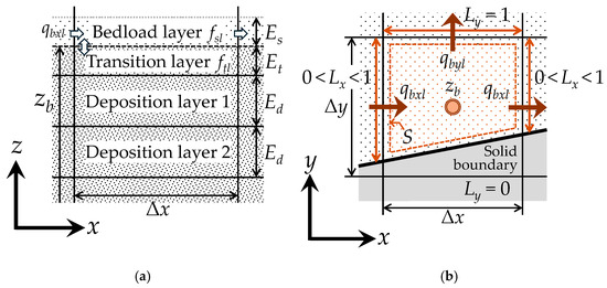
Figure 3.
Definition of variables related to the bed deformation model: (a) Each layer below the bed surface on the x–z vertical plane; (b) calculation points on the x–y horizontal plane.
The bedload layer thickness Es is given by Egashira and Ashida [52]:
where τ∗m is the dimensionless tractive force for mean grain dm; and φ is the angle of repose in water (=40° in this study).
The bedload transport rates for l-th grain in the x and y directions, qbxl and qbyl, were calculated using Ashida et al. [53]:
in which
where ζl is the angle between the direction of l-th grain movement and the x direction; ξ (=tan−1(vb/ub)) is the angle between the direction of the near-bed flow velocity and the x direction; ub and vb are the near-bed flow velocity components in the x and y directions, respectively; and θx and θy are the angle of the bed slope in the x and y directions, respectively.
The dimensionless critical tractive force on the flatbed for l-th grain τ∗cl was evaluated by the following modified Egiazaroff formula [49,54]:
where τ∗cm is the dimensionless critical tractive force on the flatbed for mean grain dm, and τ∗cm was estimated by the following Iwagaki’s formula [55]:
Various methods have been proposed to calculate near-bed flow velocities, ub and vb, within the framework of depth-integrated 2D models. For example, Yoshida and Ishikawa [56] proposed a linear approximation of the vertical velocity distribution using the depth-averaged flow velocity and its deviation. They derived new equations for the depth-averaged flow and its deviation by integrating in the depth direction using the weighted-residual method and calculated near-bed flow velocities by solving these equations. Uchida and Fukuoka [57] presented a method to calculate near-bed flow velocities by coupling the depth-averaged horizontal vorticity equation with a 2D model in which the vertical velocity distribution is assumed to be a cubic function.
However, the applicability of these methods to steep channels has not been examined. These methods increase the number of equations to be solved, potentially complicating the calculations. Therefore, to maintain the practicality—a key advantage of the 2D model—this study adopts the most common method of calculating near-bed velocities from the curvature of local streamlines (e.g., [58]). In this 2D model, near-bed flow velocities are evaluated using the following equations, based on Engelund [59]:
where αs is the angle between the primary flow direction and the x direction (=tan−1(V/U) ); and r is the radius of curvature of the depth-averaged flow. N∗ was set to 7.0 following Engelund [59].
In the 3D model, as shown in Figure 4, the flow velocities at the Δz/2 height from the bed surface in the centre of the horizontal calculation grid were defined as the near-bed flow velocities. This is because, when the bed surface crosses diagonally across an equally spaced grid, multiple computational cells containing the bed surface appear in the vertical direction, complicating the selection of the near-bed velocity, which should be defined at only one point on a horizontal calculation grid. In this study, the vertical grid size of the lowest calculation cell including the bed surface Δzb was defined as Δzb = (Azb/Vfb)Δz, and the flow velocities in the lowest cell was defined to be at a height of Δzb/2 from the bed surface (here, Azb and Vfb are the fractional area ratio in the z direction and the fractional volume ratio at the lowest cell, respectively). Then, the near-bed flow velocities at the Δz/2 height from the bed surface were obtained from the Lagrange interpolation polynomial [60] using several velocities in the upper from the bed. Referring to Figure 4, ub is calculated using the following equation:
where Δb = Δzb/Δz; u0 is the flow velocity in the x direction at the lowest calculation cell; and u+1, u+2, and u+3 are the flow velocities in the x direction in the upper cells from the lowest calculation cell.
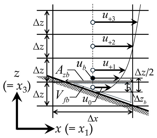
Figure 4.
Calculation points of near-bed flow velocity ub on the x–z vertical plane in the 3D model.
When the flow depth was small, and there were only three flow velocities above the bed surface, the following equation was used:
If the flow depth was small and the velocities in the upper cells from the lowest calculation cell were less than two points from the bed surface, the velocity in the lowest cell was used as the near-bed velocity. vb was also determined in a similar manner.
In addition, the friction velocity u∗ in the 3D model was calculated using the following equation, assuming that a logarithmic law holds between the bed surface and Δz/2 height point:
where u∗x and u∗y denote the shear velocities in the x and y directions, respectively.
The bed level zb was calculated using the Exner equation for total sediment transport by incorporating the FAVOR method as follows:
2.2. Boundary Conditions
In the hydraulic experiments targeted in this study, as described in Section 3.1, supercritical flow conditions were observed at both the upstream and downstream ends. Therefore, at the upstream boundary, the uniform flow depth and flow discharge per unit width observed in each experiment were imposed across the transverse direction in both hydrodynamic models. In the 3D model, the flow discharge per unit width was given as a logarithmic velocity distribution in the vertical direction. The turbulence values were given by the following equations, which were modified from the equations presented by Kuhnle et al. [61] to correspond to the SST k–ω model:
where z′ is the distance from the bed in the vertical upward direction.
The equilibrium bedload transport rate was provided at the upstream boundary to prevent bed deformation. At the downstream boundary, all physical quantities were set as free outflows in both hydrodynamic models. Both hydrodynamic models also assume a logarithmic friction resistance at the wall boundary. Furthermore, in the 3D model, the turbulence values near the wall were given by the following wall function:
At the water surface boundary in the 3D model, a free-slip condition was imposed on the flow velocities and the turbulent kinetic energy k. To avoid discontinuity of the specific turbulent dissipation rate ω at the water surface, ω was given by following equation, similar to the wall functions, based on the method of Sugiyama et al. [62]:
where ωw is the specific turbulent dissipation rate of the water surface cell; kw is the turbulent kinetic energy of the water surface cell; and Δw is the distance from the water surface to the calculation point of the water surface cell.
To consider the attenuation of vertical turbulence near the water surface, the eddy viscosity coefficient was multiplied by the attenuation function fsw given in the following equation [6,63]:
where B is the constant value of 10.
The flow depth h becomes very small immediately downstream of the structures placed in the supercritical flow fields, and in some cases, the calculation grids dry up. In n the fixed-bed experiment conducted by Michiue et al. [35], discussed in Section 3.1 and Section 4.1, drying up occurred behind a block. Therefore, the following dry-bed conditions were imposed on both flow models. In the 2D model, a minimum flow depth hmin was set, and when the flow depth of the target cell became smaller than hmin, the flow discharges per unit width (or the depth-averaged velocities) of that cell were calculated from the momentum Equations (2) and (3), excluding the advective and viscosity terms. The drying up and recovery of the flow depth were expressed by solving the continuity equation (Equation (1)). In the 3D model, the minimum flow depth hmin was set as that in the 2D model. When the flow depth of the target cell was less than hmin, both the flow depth and flow velocities of the cell were set to zero. When the water level in the surrounding cell was greater than 1.05 times hmin above the bed elevation of the dried-up cell, the flow depth of that cell was restored to hmin. Based on several calculations with various changes in calculation grid size and target conditions, hmin was determined automatically using
where min is a mathematical function to calculate the minimum value among the values within ( ); and Δx, Δy, and Δz are the calculation grid sizes in the x, y, and z directions, respectively; the grid sizes Δx, Δy, and Δz are not constant values.
In flow fields where advection dominates, such as in rivers, changes in the vertical velocity distribution are expected to be larger than those in the horizontal velocity distribution. To resolve the vertical velocity distribution, in the 3D model we set the vertical grid size Δz to approximately 1/5 to 1/3 of the horizontal grid size Δx (or Δy). In this case, the order of magnitude of hmin in the 3D model is equivalent to that of hmin in the 2D model.
2.3. Numerical Methods
The calculation flowchart for the flow and bed deformation using the 2D and 3D models is shown in Figure 5. The numerical methods used to solve the governing equations of each model are described below.
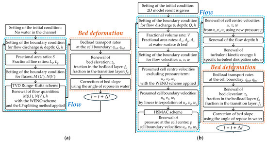
Figure 5.
Flowcharts of flow and bed deformation calculations using two hydrodynamic models: (a) 2D model; (b) 3D model (Δt is the calculation time step).
In the 2D model, a regular grid arrangement was adopted as the calculation grid, with all physical quantities defined at the cell centre, as shown in Figure 1. To discretise the advective terms in Equations (1)–(3), the fluxes defined at the cell centre were first separated using the modified Lax–Friedrich (LF) splitting method [64]. The fluxes at the cell boundaries were then computed using the fifth-order weighted essentially non-oscillatory (WENO) scheme [64,65]. The WENO scheme is a high-order, accurate shock-capturing scheme that can analyse discontinuities without requiring artificial viscosity terms. A third-order WENO scheme was applied near the wall boundaries. A sixth-order central difference method was used to discretise the pressure term, while lower-order central difference methods were applied near the walls. The viscosity term was discretised using a second-order central difference method. For time integration, the third-order total variation diminishing Runge–Kutta method [65,66] was used.
As shown in Figure 5a, the 2D model initially contained no water in the channel. The flow discharge was gradually increased from the upstream end. After increasing to a predetermined discharge, calculations were performed until a steady state was reached, that is, until the water level fluctuations almost disappeared. During this period, no bed deformation calculations were performed; the flow-only calculation was performed. After the flow reached a near-steady state, the bed deformation calculations were initiated. Subsequently, both flow and bed deformation calculations were repeated at intervals of Δt.
In the 3D model, a collocated grid arrangement was used for the calculation grid, with flow velocity components defined at both the cell centre and cell boundaries, as shown in Figure 2. As in the 2D model, the fifth-order WENO scheme was used to discretise the advective term in Equation (9). However, near the water surface and wall boundaries, the third-order WENO scheme and first-order upwind method were applied. The pressure and boundary velocities were solved using the highly simplified marker-and-cell method on a collocated grid arrangement proposed by Ushijima and Nezu [67] to satisfy the local continuity equation. A second-order central difference method was used to discretise the viscosity terms, and the vertical viscosity term was discretised implicitly. A sixth-order central difference method was applied to the pressure term, with lower-order methods used near the water surface and walls. The water surface was modelled as flat within the calculation cells, as shown in Figure 6, with its position determined using the simplified volume of fluid (VOF) method [68], which assumes only one water surface exists vertically. Additionally, the exponential method [69] was used to discretise the turbulence model in Equations (13) and (14).
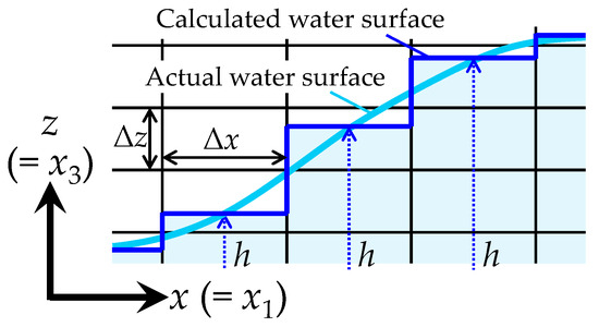
Figure 6.
Modelling of the water surface shape using the simplified VOF method in the 3D model.
The steady-state flow results obtained from the 2D model prior to bed deformation were used as the initial flow condition in the 3D model. As in the 2D model, the bed deformation calculations were not performed initially. After the flow reached a near-steady state, the bed deformation calculations were performed following the procedure outlined in Figure 5b.
In the bed deformation model, a staggered grid arrangement was used, with bed elevation defined at the cell centre and bedload in each direction defined at the cell boundaries, as shown in Figure 3b. The spatial differential terms in Equations (21) and (36) were discretised using the finite volume method, and the first-order Euler method was used for time integration. Furthermore, if the angle of the local bed slope exceeded the angle of repose in water as the bed deformation calculation progressed, the sediment instantly collapsed from the higher bed level to the lower bed level in the direction of the maximum bed slope to maintain the angle of repose in water, as shown in Figure 7 [36]. The bed levels after modification based on the angle of repose are expressed using the following equations:
where the superscripts L and H indicate the lower and higher bed level values, respectively; the superscript bars indicate before-modification values; and Δzb′ is the modification value of bed level.
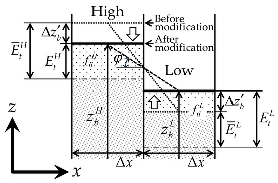
Figure 7.
Modification of local-bed slope using angle of repose in water.
During this modification process, the thickness Es, and grain-size fraction fsl of the bedload layer did not change; however, those of the transition layer at the lower bed level changed. The grain-size fraction ftl in the transition layer at the lower bed level after the sediment collapse was determined using
3. Experiments and Calculation Conditions
3.1. Overview of Experiments
In this study, numerical simulations were conducted for three hydraulic experiments performed in the same channel [35,36]. Schematics of the experimental channels are shown in Figure 8, and the experimental conditions are summarised in Table 1. A straight steel channel measuring 7.0 m in length, 0.4 m in width, and 0.4 m in depth was used. The experiments simulated conditions in which a steep channel slope and a non-overflow block on the left bank represented a constriction caused by large boulders in a mountainous river.
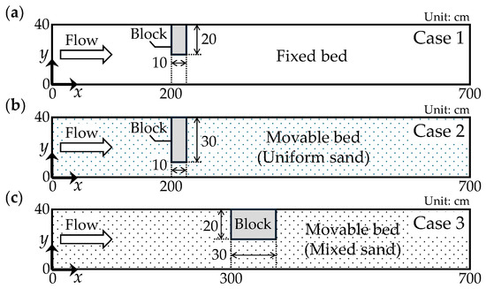
Figure 8.
Schematics of the experimental channels: (a) Fixed bed (Michiue et al. [35]); (b) movable bed with uniform sand (Nagase et al. [36]); (c) movable bed with mixed sand (Michiue et al. [35]).

Table 1.
Experimental conditions.
Case 1 (Michiue et al. [35]) was a fixed-bed experiment with a channel slope of 1/25. A block measuring 0.2 m wide, 0.1 m long, and 0.4 m high was placed on the left bank, 2.0 m from the upstream end (Figure 8a). A constant flow discharge of 0.00136 m3/s was introduced, and the flow velocity and water level were measured using an electromagnetic current meter and a servo-type water level meter, respectively. Flow velocity measurements were taken at a single point at mid-depth, excluding locations with very shallow flow.
Case 2 (Nagase et al. [36]) involved a movable bed experiment with uniform sand. A block measuring 0.3 m wide, 0.1 m long, and 0.4 m high was placed on the left bank, 2.0 m from the upstream end of a channel with a slope of 1/30 (Figure 8b). The constriction was narrow and short in the downstream direction. Uniform sand with a grain size of 7.46 mm was spread evenly, and a constant flow discharge of 0.00456 m3/s was applied. No sediment was supplied from upstream, and a downstream weir—at the same height as the initial bed—prevented bed degradation. Sediment transport ceased 10 min after discharge began, at which point velocity and water level were measured as in Case 1. The bed level was measured with a point gauge after the flow stopped.
Case 3 (Michiue et al. [35]) was another movable bed experiment, this time using mixed sand. A block measuring 0.2 m wide, 0.3 m long, and 0.4 m high was placed on the left bank, 3.0 m from the upstream end of a channel with a slope of 1/25 (Figure 8c). The constriction was relatively wide and long. Figure 9 shows the grain size distribution of the bed material used in this experiment. The mean grain size dm was calculated as the sum of the five characteristic grain sizes shown in Figure 9, each multiplied by its respective proportion. The mixed sand was laid flat, and a constant discharge of 0.00635 m3/s was applied. The upstream and downstream bed boundary conditions were identical to those in Case 2. A static equilibrium state with no observable sediment transport was reached 10 min after the start of the discharge. Flow velocity was not measured in Case 3; however, the water level, bed level, and mean grain size of the surface material were measured after flow cessation.
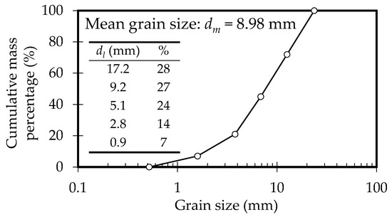
Figure 9.
Grain size distribution of bed material in experimental Case 3.
3.2. Calculation Conditions
The numerical models developed in this study introduced the FAVOR method into the governing equations so that flows and bed deformations could be smoothly analysed, even for boundary shapes that did not follow the coordinate system. To confirm the effectiveness of introducing the FAVOR method, this study conducted analyses on two channels: In Channel A, the calculation grids were aligned with the x-y coordinate system and the channel shape; and in Channel B, the grids were rotated clockwise by θ (tan θ = 1/3) from the x-y coordinate system, as shown in Figure 10. The calculation conditions are listed in Table 2. In a previous study using the presented 3D model, we conducted a sensitivity analysis on flow around a cylinder by varying the grid size [47]. The results showed that the 3D model could accurately reproduce the flow when the target structure was resolved with approximately 10 or more grids. Michiue et al. [35] and Nagase et al. [36] performed analyses using 2D models, employing grid sizes of Δx = Δy = 0.02 m. Therefore, in this study, the grid size was determined so as to resolve the blocks with approximately 10 grids, resulting in a smaller grid size than that used by Michiue et al. [35] and Nagase et al. [36]. The analyses were then performed using Channels A and B for experimental Cases 1 and 2, respectively.
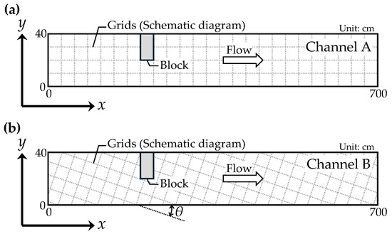
Figure 10.
Calculation channels: (a) In Channel A, the calculation grids follow the channel shape; (b) In Channel B, the calculation grids are rotated clockwise from the x-y coordinate system by an angle θ.
Table 2.
Calculation conditions.
The calculation domain was the same as that in the experiments, spanning 7 m. Manning’s roughness coefficient of the wall surface was set to 0.008 for the channel sidewalls, which were made of glass, and 0.010 for the block wall surface [70]. A detailed investigation of the effects of channel sidewall roughness on the calculation results will be considered in a future work. However, preliminary calculations using the 2D model with sidewall roughness coefficient varying between 0.008 m−1/3 s and 0.010 m−1/3 s confirmed that the result remained largely unchanged. As mentioned in Section 2.2, in the calculations for both hydrodynamic models, the sidewall Manning’s roughness coefficients were converted to equivalent roughness height using the Manning–Strickler formula, and the sidewall resistances were given using a logarithmic law at each calculation grid on the wall boundary.
As explained in Section 2.3, in the 2D model, the initial flow condition was set as no water in the channel. The flow discharge was increased from the upstream end over 10 s to a predetermined value, after which a constant discharge flowed through the channel. Because of the sufficient distance from the upstream end to the block, the influence of the inflow boundary on the calculation results can be considered negligible. The steady-state flow after 120 s from the flow-only calculation using the 2D model was used as the initial condition for the 3D model. That is, the depth-averaged flow velocity and eddy viscosity coefficient obtained from the 2D model results were uniformly distributed in the vertical direction. The repeated calculations of the bed deformation and flow were initiated after the flow-only calculation became approximately steady in both the 2D and 3D models. As in the experiment, the calculated results were output 600 s later, when the bed deformations had almost ceased.
4. Model Applications and Discussions
4.1. Case 1: Fixed-Bed Experiment
4.1.1. Comparisons of Experimental and Calculated Results
Figure 11 and Figure 12 compare the water surface profiles and depth-averaged flow velocities, respectively. While the 2D model showed an almost steady-state flow with no water surface fluctuations, the 3D model exhibited temporal fluctuations at the tip of the hydraulic jump. Therefore, the 2D model results represent instantaneous values, whereas the 3D model results represent time-averaged values over 60 s. Figure 12 presents the flow depth contours.
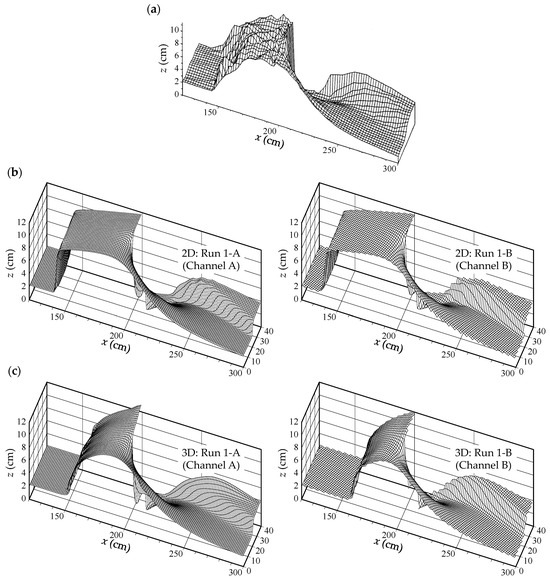
Figure 11.
Bird’s-eye view of water surfaces in Case 1: (a) Experiment (Michiue et al. [35]); (b) 2D model results (left: Channel A, right: Channel B); (c) 3D model results (left: Channel A, right: Channel B).
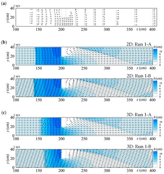
Figure 12.
Depth-averaged flow velocity vectors in Case 1: (a) Experiment (Michiue et al. [35]), (b) 2D model results (upper: Channel A, lower: Channel B); (c) 3D model results (upper: Channel A, lower: Channel B).
Figure 11a shows that, in the experiment, a hydraulic jump occurred near x = 150 cm, and the flow depth rapidly increased from 2 cm to approximately 10 cm. The flow depth decreased downstream of x = 200 cm, where the block was installed. At the left bank sidewall downstream of the block, the collision of backward flow caused the formation of shock waves and an increase in flow depth. The computational results in Figure 11b,c closely match the experimental observations. However, in the 2D model results (Figure 11b), although no numerical oscillation occurred, the hydraulic jump appeared at approximately x = 140 cm, earlier than in the experiment. Additionally, the water surface shape following the jump was flatter than in the experimental result. By contrast, the 3D model results (Figure 11c) closely reproduced the experimental outcomes. In particular, the 3D simulation for channel A (Figure 11c, left, 3D: Run 1-A) accurately replicated the hydraulic jump location and upstream water surface profile, as well as the flow pattern near the left-bank sidewall downstream of the block. Regarding differences between channel geometries, the 2D model (Figure 11b) showed that Run 1-B experienced a slightly earlier hydraulic jump than Run 1-A. Conversely, the 3D model (Figure 11c) showed that Run 1-B produced a later hydraulic jump, around x = 160 cm, and a shorter jump length than Run 1-A. These discrepancies may be attributed to the reduced accuracy of the finite difference method near the wall boundary. However, the differences are minor. Therefore, by introducing the FAVOR method, the presented numerical models achieved nearly identical water surface results, even when the channel geometry did not align with the coordinate system.
Regarding the flow velocities shown in Figure 12a, the velocity decreased after x = 150 cm, where the hydraulic jump occurred, and a vortex formed near the left-bank sidewall just upstream of the block. Additionally, certain regions immediately downstream of the block were excluded from measurement owing to extremely shallow flow depth. The simulation results (Figure 12b,c) show that no vortex formed on the left-bank sidewall upstream of the block. However, both models successfully reproduced key experimental trends, such as the velocity reduction due to the hydraulic jump, lateral flow spreading toward the left bank after the block, and shock wave generation. Although the hydraulic jump occurred earlier in the 2D model than in both the experimental and 3D models, the overall flow patterns were similar. In summary, for flow-only predictions involving supercritical flow in steep channels, the 2D model provides sufficient accuracy for practical use, as model differences remain small owing to the shallow flow depth. Furthermore, both models using channel B reproduced smooth flow patterns consistent with the boundary shape owing to the use of the FAVOR method and were nearly identical to those obtained for channel A. The introduction of the FAVOR method confirms that the presented numerical models can reproduce flow velocities consistently, regardless of coordinate system orientation.
4.1.2. Internal Flow by the 3D Hydrodynamic Model
Figure 13 shows the internal flow structure, including the hydraulic jump along the longitudinal direction of the channel, obtained from the 3D model results. These results are time-averaged over 60 s.
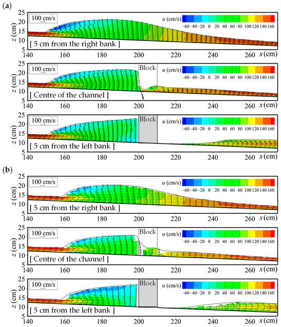
Figure 13.
Flow velocity vectors in longitudinal sections obtained using the 3D model in Case 1: (a) Run 1-A (Channel A); (b) Run 1-B (Channel B).
As presented in Table 1, the inflow Froude number in Case 1 was 3.37, which corresponds to the condition for an oscillating hydraulic jump in a flat channel [71]. In such a jump, a backflow roller forms on the water surface as the main flow plunges to the channel bed, followed by an oscillatory jet that resurfaces and recirculates. In the 3D simulation, temporal fluctuations in the water surface were observed at the onset of the hydraulic jump. Figure 13 illustrates the formation of a backflow roller at the water surface, confirming that the proposed 3D model can reproduce key experimental characteristics of oscillating hydraulic jumps.
The figure also shows a sharp drop in flow depth near the block located at the centre of the channel. Flow depth becomes extremely shallow, and the channel bed dries out immediately downstream of the block along the left bank. Although the experiment involved severe hydraulic conditions—high velocities and significant water surface fluctuations—the proposed 3D model achieved stable simulation results.
Regarding differences between computational channels A and B, the overall flow patterns were nearly identical, with only minor variations in the hydraulic jump location and the size of the backflow roller. In summary, the presented 3D model produces stable and consistent results for complex flow fields involving hydraulic jumps, even when the channel geometry is not aligned with the coordinate system. Although the computational load of 3D models is greater than that of 2D models, the presented 3D model can provide much more detailed information about internal flow structures in supercritical flow fields than the 2D model.
4.2. Case 2: Movable Bed with Uniform-Sand Experiment
4.2.1. Comparisons of Experimental and Calculated Results
Figure 14 shows a contour plot of bed deformation. The calculation results in Figure 14b,c also include near-bed flow velocity vectors.
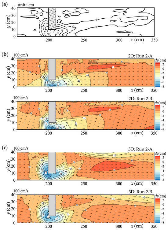
Figure 14.
Bed deformation contours in Case 2: (a) Experiment (Nagase et al. [36]); (b) 2D model results (upper: Channel A, lower: Channel B); (c) 3D model results (upper: Channel A, lower: Channel B).
The experimental result in Figure 14a indicates that a mortar-shaped local scour, approximately 10 cm deep, developed at the tip of the block at x = 205 cm, followed by a 2 cm-deep water path extending downstream. The calculation results from both models (Figure 14b,c) successfully reproduced the local scour at the block tip. However, the maximum scour depths were shallower than in the experiment: −8.3 cm for Channel A and −8.1 cm for Channel B in the 2D model, and −8.5 cm and −8.2 cm for Channels A and B in the 3D model, respectively. The locations of maximum scour differed: along the right-bank sidewall in the 2D model and upstream of the block tip in the 3D model, with the latter better reproducing the experimental observation. Additionally, the 2D model failed to reproduce the downstream water path, as erosion occurred primarily along the right-bank sidewall. By contrast, the 3D model captured erosion extending from the right- to the left-bank downstream of the block, although the resulting water path was less distinct than in the experiment.
Figure 15 compares experimental and calculated water surface profiles and bed levels in transverse sections between x = 190 and 240 cm, using Channel A results for both models.
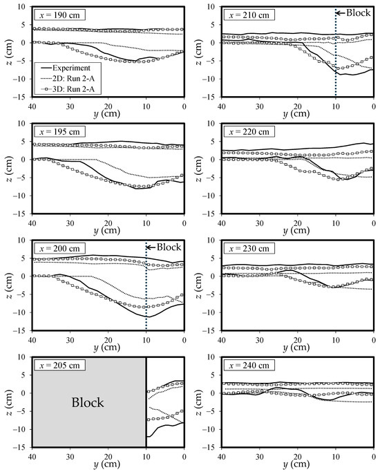
Figure 15.
Comparisons of measured and calculated water surfaces and bed levels at transverse sections in experimental Case 2.
Upstream of the block (from x = 190 to 200 cm), the 3D model closely matched the experimental water surface and bed levels, whereas the 2D model underestimated the scour depth. At x = 205 cm, neither model captured the full scour depth, but the 2D model produced a bed sloping to the right, while the 3D model showed a slope to the left—matching the experiment. Further downstream (from x = 210 to 240 cm), the 3D model reproduced the downstream migration of the scour zone toward the left bank. By contrast, the 2D model consistently localised scour on the right bank and significantly underestimated the water surface owing to excessive scour.
Thus, the 3D model clearly outperformed the 2D model in simulating bed deformation, even in shallow-water flow fields where subcritical and supercritical flows coexist. This is because the 2D model cannot adequately reproduce near-bed flows that govern sediment transport direction, even under shallow conditions. As shown in Figure 14c, near-bed flows in the 3D model radiated from the deepest point in the scour hole. By contrast, Figure 14b shows that the 2D model produced near-bed flows from upstream toward the deepest point, then deflected toward the left bank at the block tip. This direction was opposite to that of the 3D model, and no directional change occurred when N∗ = 0.0 in Equation (30). Furthermore, downstream of the block, the 2D model showed weak lateral spreading of flow toward the left bank. These discrepancies likely explain why the 2D model struggled to reproduce both the maximum scour location and the downstream water path. Nonetheless, the maximum scour depths predicted by both models were not significantly different. When channel constrictions are narrow and short in the downstream direction, a 2D model may still be adequate to predict the approximate scour shape and depth.
With respect to channel differences, almost no variation was observed between Channels A and B in the 2D model (Figure 14b). However, in the 3D model (Figure 14c), the scour hole at the block tip was slightly smaller in 3D: Run 2-B (Channel B) than in Run 2-A. This produced minor changes in downstream flow direction and topography. As in Case 1, these differences likely reflect the effects of reduced accuracy of the finite difference method near the wall boundary in the 3D model. Nevertheless, overall bed deformation was nearly identical between the two channels, and smooth deformation was achieved near boundaries such as sidewalls and block faces. These findings confirm the effectiveness of introducing the FAVOR method into the bed deformation model.
4.2.2. Internal Flow by the 3D Model
The flow patterns responsible for local scour were analysed using the 3D model results. Figure 16 shows the internal flow within the scour hole, calculated using Channel A.
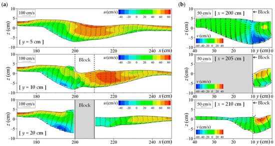
Figure 16.
Flow velocity vectors obtained by the 3D model result (Run 2-A) in Case 2: (a) Longitudinal sections; (b) transverse sections.
Across all panels in Figure 16, the 3D model produced smooth flows along the bed surface by incorporating the FAVOR method, even for geometries not aligned with Cartesian coordinate system. In terms of flow behaviour, Figure 16a reveals a horseshoe vortex forming in the scour hole upstream of the block. At x = 200 cm (just upstream of the block), Figure 16b shows the vortex deflecting toward the right bank and descending toward the bed. At x = 205 cm, a counterclockwise secondary flow developed, leading to the maximum scour depth at the block tip. Such complex flow structures are difficult to capture with a 2D model, which explains its limitations in reproducing the experimental results. Even in shallow flow conditions where subcritical and supercritical flows coexist, complex 3D flow structures form within the domain. This underscores the advantage of using a 3D model for accurately predicting bed deformation. The presented 3D model can represent such complex flows that cause local scour around structures.
4.3. Case 3: Movable Bed with Mixed-Sand Experiment
4.3.1. Comparisons of Experimental and Calculated Results
Figure 17 and Figure 18 show the bed deformation contours and mean grain size distributions of the bed surface, respectively. The calculations were performed using Channel A. Figure 17b,c also present the near-bed flow velocity vectors.
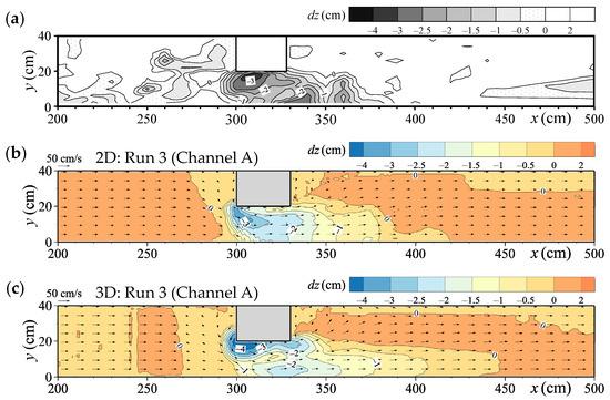
Figure 17.
Bed deformation contours in Case 3: (a) Experiment (Michiue et al. [35]); (b) 2D model results; (c) 3D model results.
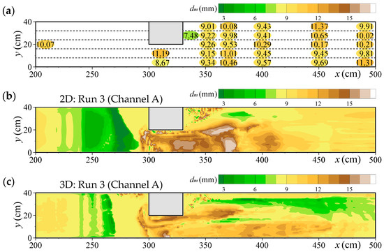
Figure 18.
Mean grain size distributions of the bed surface in Case 3: (a) Experiment (Michiue et al. [35]); (b) 2D model results; (c) 3D model results.
First, the amount of bed deformation is discussed. The experimental result in Figure 17a indicates that bed deformation was mainly concentrated within the constriction, where the block was installed. Local scouring occurred at two specific locations: on the block side at x = 310 cm, and along the right bank of the channel at x = 330–340 cm. The corresponding scour depths were approximately −4 cm at the block side and −3 cm along the right bank. In the 2D model (Figure 17b), local scour occurred only at one location—the upstream corner of the block—and the maximum scour depth was −3.3 cm, which was smaller than in the experimental results. By contrast, the 3D model (Figure 17c) reproduced local scouring at two locations: at the block side at x = 305 cm and at the right bank at x = 320–330 cm, which closely resembles the experimental observations. The scour depths estimated by the 3D model were −4.7 cm at the block side and −2.3 cm at the right bank, respectively. Although these values differ somewhat from the experimental depths, the trend of deeper scouring at the block side compared to that at the right bank was successfully reproduced.
Next, the mean grain size distribution of the bed surface is examined. The initial mean grain size before flow was 8.98 mm across the entire channel bed, including the surface. The experimental result in Figure 18a indicates that the mean grain size became coarser after flow exposure. Although generalisation is difficult owing to variations in the experimental data, coarsening occurred in the constricted scour zone because finer grains were transported downstream, whereas the mean grain size became finer immediately downstream of the block owing to deposition of fine grains. The numerical results of both models show a coarser mean grain size in the areas where scouring occurred, which is consistent with the trend observed in the experiment. However, the 2D model (Figure 18b) showed a stronger coarsening tendency than the 3D model, with a broader area exhibiting mean grain sizes of 15 mm or greater. By contrast, the 3D model (Figure 18c) predicted that only a limited region exceeded 15 mm, and the overall mean grain size was around 10 mm, which is closer to the experimental results.
Figure 19 presents a comparison of the experimental and calculated water surface profiles and bed levels in the longitudinal direction of the channel. In the longitudinal section at y = 5 cm (Figure 19a), both the 2D and 3D models showed a minor scour at the block location (around x = 330 cm) but failed to reproduce sediment deposition at x = 400 cm. As a result, the models could not replicate the water level rise caused by flow damming downstream of the block. Similarly, in the longitudinal section at y = 20 cm (Figure 19b), both models failed to simulate the sediment deposition between x = 400–430 cm, resulting in a poorly reproduced water surface profile downstream of the block. However, in the region from the upstream end of the channel to x = 350 cm, including the scour zone in front of the block, the 3D model produced a bed profile and water surface that closely matched the experimental observations. By contrast, the 2D model predicted shallower scour and displayed poor agreement with the experimental water surface.
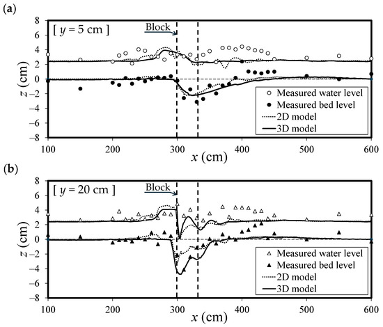
Figure 19.
Comparisons of measured and calculated water surfaces and bed levels in the longitudinal sections: (a) y = 5 cm; (b) y = 20 cm.
As described above, clear differences are observed between the hydrodynamic models when analysing an experiment involving a long block in the flow direction and a domain with coexisting subcritical and supercritical flow. In this case, the 3D model proved superior to the 2D model. Although the 2D model could approximately predict the general area where scour occurred in the constriction, it could not reproduce the presence of two separate scour zones or the accurate scour depths. By contrast, the 3D model successfully predicted the occurrence of local scour at two locations, along with reasonably accurate depths and grain size distributions on the bed surface.
4.3.2. Internal Flow in a Constricted Section
The mechanisms responsible for the occurrence of local scour at the two sites, at the block side and the right bank of the constriction, are investigated using the 3D model results. Figure 20 shows the transverse flows at the respective sections where local scours developed.
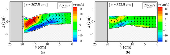
Figure 20.
Flow velocity vectors in the transverse sections obtained by the 3D model result: (a) x = 307.5 cm (scour hole on the block side); (b) x = 322.5 cm (scour hole on the right bank side).
In the transverse section where scour occurred on the block side (Figure 20a), a counterclockwise secondary flow developed in the scour hole. This secondary flow is similar in structure to that observed in Case 2 (see Figure 16b). The vortex formed by the secondary flow had a vertical scale comparable to the flow depth. Because the water surface width was wider than the flow depth and there was sufficient lateral space along the right bank, a near-bed flow toward the right bank was generated. In the transverse section where scour developed along the right bank (Figure 20b), a near-bed flow toward the left bank was observed in the direction opposite to the previous secondary flow. The combined effects of these transverse flows resulted in a meandering near-bed flow within the constriction (Figure 17c). Flow moved from the upstream corner of the block to the right bank, and then from the scour zone on the right bank toward the left bank. The development of these transverse and meandering near-bed flows indicates that the dual scour pattern arose because of complex secondary flow structures. Such flow behaviour is likely to occur when the channel width is larger than the flow depth in steep, constricted sections of a river channel. It is clear that the 2D model which deals with depth-averaged flows has difficulty predicting such complex 3D flows and therefore could not reproduce the local scour at two locations.
5. Conclusions
This study aimed to clarify the suitability and differences in the numerical simulation results between a 2D shallow-water hydrodynamic model and a 3D hydrodynamic model for simulating flow and local scour around a structure in a supercritical flow field on a steep channel. Flow and mixed-sand bed deformation models using the FAVOR method were developed and applied to hydraulic experiments under supercritical flow conditions in steep channels. In addition, analyses were conducted for channels aligned and non-aligned with the coordinate system to assess the effect of introducing the FAVOR method.
For flow analyses involving hydraulic jumps, the 3D model better reproduced the experimental results, such as hydraulic jump length and water surface shape. However, in purely supercritical flow fields with shallow depths, both models produced similar results, suggesting that the 2D model is sufficient for predicting flow in such cases.
In the analysis of uniform-sand bed deformation with short block lengths, the 3D model more accurately reproduced the scour shape and the location of the maximum scour depth. This suggests that the 3D model is more suitable for predicting bed deformation in steep, supercritical flow conditions. Still, for narrow and short constrictions, the 2D model may be sufficient for estimating flow and approximate local scour.
The FAVOR method enabled both models to simulate smooth flows and bed deformation patterns that conformed to complex channel and structure shapes, even when these did not align with the Cartesian coordinate system.
In the analysis of mixed-sand bed deformation with long block lengths, the 2D model failed to reproduce the twin scour features on both banks of the constriction. By contrast, the 3D model captured this phenomenon and yielded a mean grain size distribution closer to experimental observations. Thus, in wider and longer constrictions, the 2D model may lack the capacity to accurately predict local scouring and bed deformation.
The findings of this study demonstrate the advantages of the 3D model and the applicability of the 2D model. Specifically, the findings can assist in selecting models for predicting flow and bed deformation when aiming to create varied flows and pools suitable as habitats for organisms by installing structures such as groins or large boulders in supercritical flow fields in the middle and upper reaches of rivers. The 3D model developed in this study can be used for analysing the topographical changes caused by tsunami run-up in supercritical flow conditions.
This study was limited in its application and examination to the laboratory-scale flow fields. In previous studies [48,72], we examined the reproducibility of subcritical flow fields of actual rivers using both the 2D and 3D models; however, these studies did not examine supercritical flow fields. In this study, the effects of parameter changes in the bed deformation model were not sufficiently investigated. Therefore, future work will investigate flow and bed deformation in supercritical flow fields at the actual river scale, as well as clarify the effects of model parameter modifications on analysis results.
Funding
This study was supported in part by the Japan Society for the Promotion of Science (JSPS) KAKENHI Grant Number 24K07683.
Data Availability Statement
The original contributions presented in this study are included in the article. Further inquiries can be directed to the corresponding author.
Acknowledgments
The author express their gratitude to the anonymous reviewers.
Conflicts of Interest
The author declares no conflicts of interest.
Abbreviations
The following symbols are used in this manuscript:
| a1 | turbulence constant (-) |
| A(i) | fractional area ratio at the boundary of the calculation grid in the xi direction (-) |
| Azb | fractional area ratio in the z direction in the lowest calculation cell (-) |
| B | coefficient of the attenuation function for the eddy viscosity coefficient (-) |
| cs | sediment concentration in the bedload layer (-) |
| Cf | resistance coefficient (-) |
| dl | diameter for the l-th grain (m) |
| dm | mean grain size in the bed surface material (m) |
| Ed | deposition layer thickness (m) |
| Es | bedload layer thickness (m) |
| Et | transition layer thickness (m) |
| Fr | Froude number (-) |
| F2 | blending function (-) |
| fsl | fraction of l-th grain in the bedload layer (-) |
| ftl | fraction of l-th grain in the transition layer (-) |
| ftlL, ftlH | fraction of l-th grain in the transition layer in the lower and upper beds, respectively (-) |
| g | gravitational acceleration (m s−2) |
| h | flow depth (m) |
| hmin | minimum flow depth (m) |
| h0 | uniform flow depth (m) |
| i | subscripts; 1, 2, 3 (-) |
| j | dummy indices; 1, 2, 3 (-) |
| k | turbulent kinetic energy (m2 s−2) |
| kh | depth-averaged turbulent kinetic energy (m2 s−2) |
| kL | lift-drag ratio (-) |
| ks | equivalent sand roughness (m) |
| kw | turbulent kinetic energy at the water surface cell (m2 s−2) |
| Kcl | slope factor for the l-th grain (-) |
| l | number of grain sizes of mixed-sand (-) |
| Lx, Ly | fractional line ratios at the boundary of a horizontal calculation cell in the x and y directions, respectively (-) |
| M, N | flow discharges per unit width in the x and y directions, respectively (m2 s−1) |
| N | Manning’s roughness coefficient (m−1/3 s) |
| N∗ | coefficient for secondary flow strength (-) |
| P | pressure (Pa) |
| Q | discharge (m3 s−1) |
| qbl | bedload transport rate for the l-th grain in the primary flow direction (m2 s−1) |
| qbxl, qbyl | bedload transport rates for the l-th grain per unit width in the x and y directions, respectively (m2 s−1) |
| r | radius of curvature of the depth-averaged flow (m) |
| s | specific gravity of sediment in water (-) |
| S | fractional area ratio in a horizontal calculation cell (-) |
| Sij | mean strain-rate tensor (s−1) |
| St | absolute value of Sij (s−1) |
| t | time (s) |
| ub, vb | near-bed flow velocity components in the x and y directions, respectively (m s−1) |
| ui | flow velocity component in the xi direction (m s−1) |
| u0 | flow velocity in the x direction at the lowest calculation cell (m s−1) |
| u+1, u+2, u+3 | flow velocities in the x direction in the upper cells from the lowest calculation cell (m s−1) |
| u∗ | shear velocity (m s−1) |
| u∗x, u∗y | shear velocities in the x and y directions, respectively (m s−1) |
| U, V | depth-averaged flow velocity components in the x and y directions, respectively (m s−1) |
| Vf | fractional volume ratio in a calculation cell (-) |
| Vfb | fractional volume ratio at the lowest calculation cell (-) |
| x | longitudinal direction for a main flow (m) |
| x1, x2, x3 | x, y, z in Cartesian coordinates (m) |
| y | transverse direction for a main flow (m) |
| z | vertical direction for a main flow (m) |
| z′ | distance from the bed in the vertical upward direction (m) |
| zb | bed level (m) |
| higher bed levels before and after bed slope modification, respectively (m) | |
| lower bed levels before and after bed slope modification, respectively (m) | |
| αs | angle between the primary flow direction and the x direction (-) |
| α1, α2, β1, β2, β* | turbulence constants (-) |
| γl | angle between the direction of l-th grain movement and the direction of maximum bed lope (-) |
| δ | Kronecker’s delta (-) |
| Δ | distance from the solid wall boundary to the nearest calculation point (m) |
| Δw | distance from the water surface to the calculating point of the water surface cell (m) |
| Δt | calculation time step (s) |
| Δx, Δy, Δz | calculation grid sizes in x, y, and z directions, respectively (m) |
| Δzb | vertical grid size of the lowest calculation cell including the bed surface (m) |
| Δz′b | modification value of bed level related to angle of repose in water (m) |
| ζl | angle between the direction of l-th grain movement and the x direction (-) |
| θb | angle of the maximum local-bed slope (-) |
| θx, θy | angle of the bed slope in the x and y directions, respectively (-) |
| κ | von Karman constant (-) |
| λ | porosity of the bed material (-) |
| μs | static friction coefficient (-) |
| ν | kinematic viscosity coefficient (m2 s−1) |
| νh | depth-averaged eddy viscosity coefficient (m2 s−1) |
| νt | eddy viscosity coefficient (m2 s−1) |
| ξ | angle between the direction of the near-bed flow velocity and the x direction (-) |
| ρ | density of fluid (kg m−3) |
| σ | density of sediment (kg m−3) |
| σk1, σk2, σω1, σω2 | turbulence constants (-) |
| τbx, τby | bottom shear stress components in the x and y directions, respectively (Pa) |
| τ∗cl | dimensionless critical tractive force on the flatbed for grain dl (-) |
| τ∗cm | dimensionless critical tractive force on the flatbed for mean grain dm (-) |
| τ∗l | dimensionless tractive force for grain dl (-) |
| τ∗m | dimensionless tractive force for mean grain dm (-) |
| φ | angle of repose in water (-) |
| Ψl | angle between the direction of l-th grain movement and the direction of the near-bed flow velocity (-) |
| ω | specific turbulent dissipation rate (s−1) |
| ωw | specific turbulent dissipation rate at the water surface cell (s−1) |
References
- Locke, H.; Rockström, J.; Bakker, P.; Bapna, M.; Gough, M.; Hilty, J.; Lambertini, M.; Morris, J.; Rodriguez, C.M.; Samper, C.; et al. A Nature-Positive World: The Global Goal for Nature. Available online: https://www.nature.org/content/dam/tnc/nature/en/documents/NaturePositive_GlobalGoalCEO.pdf (accessed on 25 September 2025).
- Soda, R.; Yuhora, K. What was the aim of “Nature-Oriented River Work”? E-J. GEO 2012, 7, 147–157, (In Japanese with English abstract). [Google Scholar] [CrossRef][Green Version]
- Ministry of Land, Infrastructure, Transport and Tourism of Japan. Neicha-Pojithibu wo Jitsugensuru Kawazukuri wo Susumemasu [We Will Promote River Works That Realizes the Nature-Positive]. Available online: https://www.mlit.go.jp/report/press/mizukokudo04_hh_000236.html (accessed on 25 September 2025). (In Japanese)[Green Version]
- Olsen, N.R.B.; Melaaen, M.C. Three-dimensional calculation of scour around cylinders. J. Hydraul. Eng. 1993, 119, 1048–1054. [Google Scholar] [CrossRef]
- Olsen, N.R.B.; Kjellesvig, H.M. Three-dimensional numerical flow modeling for estimation of maximum local scour depth. J. Hydraul. Res. 1998, 36, 579–590. [Google Scholar] [CrossRef]
- Nagata, N.; Hosoda, T.; Nakato, T.; Muramoto, Y. Three-dimensional numerical model for flow and bed deformation around river hydraulic structures. J. Hydraul. Eng. 2005, 131, 1074–1087. [Google Scholar] [CrossRef]
- Roulund, A.; Sumer, B.M.; Fredsøe, J.; Michelsen, J. Numerical and experimental investigation of flow and scour around a circular pile. J. Fluid Mech. 2005, 534, 351–401. [Google Scholar] [CrossRef]
- Yu, P.; Xu, S.; Chen, J.; Zhu, L.; Zhou, J.; Yu, L.; Sun, Z. Three-dimensional numerical modeling of local scour around bridge foundations based on an improved wall shear stress model. J. Mar. Sci. Eng. 2024, 12, 2187. [Google Scholar] [CrossRef]
- Zhang, H.; Nakagawa, H.; Ishigaki, T.; Muto, Y.; Baba, Y. Three-dimensional mathematical modeling of local scour. J. Appl. Mech. 2005, 8, 803–812. [Google Scholar] [CrossRef][Green Version]
- Han, X.; Lin, P.; Parker, G. Numerical modelling of local scour around a spur dike with porous media method. J. Hydraul. Res. 2022, 60, 970–995. [Google Scholar] [CrossRef]
- Han, X.; Parker, G.; Lin, P. High-fidelity numerical study of the effect of wing dam fields on flood stage in rivers. Water Resour. Res. 2025, 61, e2024WR037852. [Google Scholar] [CrossRef]
- Zhao, M.; Cheng, L.; Zang, Z. Experimental and numerical investigation of local scour around a submerged vertical circular cylinder in steady currents. Coast. Eng. 2010, 57, 709–721. [Google Scholar] [CrossRef]
- Khosronejad, A.; Kang, S.; Sotiropoulos, F. Experimental and computational investigation of local scour around bridge piers. Adv. Water Resour. 2012, 37, 73–85. [Google Scholar] [CrossRef]
- Hurtado-Herrera, M.; Zapata, M.U.; Hammouti, A.; Van Bang, D.P.; Zhang, W.; Nguyen, K.D. Numerical investigation of the scour around a diamond-and square-shaped pile in a narrow channel. Ocean. Eng. 2024, 309, 118374. [Google Scholar] [CrossRef]
- Jia, Y.; Altinakar, M.; Guney, M.S. Three-dimensional numerical simulations of local scouring around bridge piers. J. Hydraul. Res. 2018, 56, 351–366. [Google Scholar] [CrossRef]
- Quezada, M.; Tamburrino, A.; Niño, Y. Numerical simulation of scour around circular piles due to unsteady currents and oscillatory flows. Eng. Appl. Comput. Fluid Mech. 2018, 12, 354–374. [Google Scholar] [CrossRef]
- Afzal, M.S.; Bihs, H.; Kamath, A.; Arntsen, Ø.A. Three-dimensional numerical modeling of pier scour under current and waves using level-set method. J. Offshore Mech. Arct. Eng. 2015, 137, 032001. [Google Scholar] [CrossRef]
- Gautam, S.; Dutta, D.; Bihs, H.; Afzal, M.S. Three-dimensional computational fluid dynamics modelling of scour around a single pile due to combined action of the waves and current using Level-Set method. Coast. Eng. 2021, 170, 104002. [Google Scholar] [CrossRef]
- Esmaeili, T.; Dehghani, A.A.; Zahiri, A.R.; Suzuki, K. 3D Numerical simulation of scouring around bridge piers (Case Study: Bridge 524 crosses the Tanana River). World Acad. Sci. Eng. Technol. Int. J. Civ. Environ. Eng. 2009, 3, 422–426. [Google Scholar]
- Sumer, B.M. Mathematical modelling of scour: A review. J. Hydraul. Res. 2007, 45, 723–735. [Google Scholar] [CrossRef]
- Lai, Y.G.; Liu, X.; Bombardelli, F.A.; Song, Y. Three-dimensional numerical modeling of local scour: A state-of-the-art review and perspective. J. Hydraul. Eng. 2022, 148, 03122002. [Google Scholar] [CrossRef]
- Choufu, L.; Abbasi, S.; Pourshahbaz, H.; Taghvaei, P.; Tfwala, S. Investigation of flow, erosion, and sedimentation pattern around varied groynes under different hydraulic and geometric conditions: A numerical study. Water 2019, 11, 235. [Google Scholar] [CrossRef]
- Gupta, L.K.; Pandey, M.; Raj, P.A. Numerical modeling of scour and erosion processes around spur dike. Clean–Soil Air Water 2025, 53, 2300135. [Google Scholar] [CrossRef]
- Yan, X.; Mohammadian, A.; Rennie, C.D. Numerical modeling of local scour due to submerged wall jets using a strict vertex-based, terrain conformal, moving-mesh technique in OpenFOAM. Int. J. Sediment Res. 2020, 35, 237–248. [Google Scholar] [CrossRef]
- Chippada, S.; Ramaswamy, B.; Wheeler, M.F. Numerical simulation of hydraulic jump. Int. J. Numer. Methods Eng. 1994, 37, 1381–1397. [Google Scholar] [CrossRef]
- Bayon, A.; Valero, D.; García-Bartual, R.; Vallés-Morán, F.J.; López-Jiménez, P.A. Performance assessment of OpenFOAM and FLOW-3D in the numerical modeling of a low Reynolds number hydraulic jump. Environ. Model. Softw. 2016, 80, 322–335. [Google Scholar] [CrossRef]
- Martínez, B.; Guerra, M.; Riviere, N.; Mignot, E.; Link, O. RANS simulation of supercritical open channel flows around obstacles. J. Hydraul. Res. 2025, 63, 1–14. [Google Scholar] [CrossRef]
- Link, O.; Mignot, E.; Roux, S.; Camenen, B.; Escauriaza, C.; Chauchat, J.; Brevis, W.; Manfreda, S. Scour at bridge foundations in supercritical flows: An analysis of knowledge gaps. Water 2019, 11, 1656. [Google Scholar] [CrossRef]
- Kusakabe, S.; Michiue, M.; Hinokidani, O.; Fujita, M. A numerical simulation of flow pattern and bed variation on widening steep slope channels. In Proceedings of the XXX IAHR Congress, Thessaloniki, Greece, 24–29 August 2003; Theme D. pp. 335–342. [Google Scholar]
- Wu, W. Depth-averaged two-dimensional numerical modeling of unsteady flow and nonuniform sediment transport in open channels. J. Hydraul. Eng. 2004, 130, 1013–1024. [Google Scholar] [CrossRef]
- Yoshitake, H.; Tsubaki, R.; Kawahara, Y. Accuracy of estimated flood discharge hydrograph in steep river by 2-D numerical simulation. J. Jpn. Soc. Civ. Eng. Ser. A2 (Appl. Mech.) 2011, 67, I_683–I_691, (In Japanese with English abstract). [Google Scholar] [CrossRef][Green Version]
- Juez, C.; Murillo, J.; García-Navarro, P. A 2D weakly-coupled and efficient numerical model for transient shallow flow and movable bed. Adv. Water Resour. 2014, 71, 93–109. [Google Scholar] [CrossRef]
- Chang, K.H.; Wu, Y.T.; Wang, C.H.; Chang, T.J. A new 2D ESPH bedload sediment transport model for rapidly varied flows over mobile beds. J. Hydrol. 2024, 634, 131002. [Google Scholar] [CrossRef]
- Kinose, K.; Taruya, H.; Ikeda, H. Analyses of water surface disturbance and bottom transformation due to pile-like construction on supercritical flow. Trans. Jpn. Soc. Irrig. Drain. Reclam. Eng. 1990, 1990, 123–131, (In Japanese with English abstract). [Google Scholar] [CrossRef]
- Michiue, M.; Hinokidani, O.; Fujii, T.; Matsumoto, K. Jyou–syaryu konzaika no kongousya kasyouhendou simyureisyon [Numerical simulation of bed variation with non-uniform sediment transport in subcritical and supercritical coexisting flow field]. In Proceedings of the 48th Research Presentation, Chugoku Regional Branch Office, Japan Society of Civil Engineers, National Institute of Technology, Tokuyama College, Yamaguchi, Japan, 25–26 May 1996; Volume 48, pp. 207–208. Available online: http://library.jsce.or.jp/jsce/open/00549/1996/48-0207.pdf (accessed on 25 September 2025). (In Japanese).
- Nagase, K.; Michiue, M.; Hinokidani, O. Simulation of bed evolution around contraction in mountainous river. Annu. J. Hydraul. Eng. Jpn. Soc. Civ. Eng. 1996, 40, 887–892, (In Japanese with English abstract). [Google Scholar] [CrossRef][Green Version]
- Pan, C.; Huang, W. Numerical modeling of tsunami wave run-up and effects on sediment scour around a cylindrical pier. J. Eng. Mech. 2012, 138, 1224–1235. [Google Scholar] [CrossRef]
- Wu, W.; Wang, S.S.Y. Prediction of local scour of non-cohesive sediment around bridge piers using FVM-based CCHE2D Model. In Proceedings of the 1st International Conference on Scour of Foundations, Texas A&M University, College Station, TX, USA, 17–20 November 2002; pp. 1176–1180. [Google Scholar]
- Martínez-Aranda, S.; Murillo, J.; García-Navarro, P. Comparison of new efficient 2D models for the simulation of bedload transport using the augmented roe approach. Adv. Water Resour. 2021, 153, 103931. [Google Scholar] [CrossRef]
- Lane, S.N.; Bradbrook, K.F.; Richards, K.S.; Biron, P.A.; Roy, A.G. The application of computational fluid dynamics to natural river channels: Three-dimensional versus two-dimensional approaches. Geomorphology 1999, 29, 1–20. [Google Scholar] [CrossRef]
- Abdo, K.; Riahi-Nezhad, C.K.; Imran, J. Steady supercritical flow in a straight-wall open-channel contraction. J. Hydraul. Res. 2019, 57, 647–661. [Google Scholar] [CrossRef]
- Hyogo Prefecture, Japan. Kouseido Sanjigen Chiri-Kukan Deita no Katsuyou [Utilization of High-Precision 3D Geospatial Data]. Available online: https://web.pref.hyogo.lg.jp/kk26/hyogo-geo.html (accessed on 25 September 2025). (In Japanese)
- Hirt, C.W.; Sicilian, J.M. A porosity technique for the definition obstacle in rectangular cell meshes. In Proceedings of the International Conference on Numerical Ship Hydrodynamics, 4th, National Academy of Science, Washington, DC, USA, 24–27 September 1985; pp. 1–19. [Google Scholar]
- Uchida, T.; Kawahara, Y.; Kinashi, Y.; Ito, Y. A high-resolution simulator for inundation flows in urban districts and its application to takehara city due to storm surge. Annu. J. Hydraul. Eng. Jpn. Soc. Civ. Eng. 2007, 51, 517–522, (In Japanese with English abstract). [Google Scholar] [CrossRef][Green Version]
- Nikuradse, J. Laws of flow in rough pipes (Translation of the 1933 paper). In Technical Memorandum, 1292; National Advisory Committee for Aeronautics: Washington, DC, USA, 1950; pp. 1–62. [Google Scholar][Green Version]
- Menter, F.R. Two-equation eddy-viscosity turbulence models for engineering applications. AIAA J. 1994, 32, 1598–1605. [Google Scholar] [CrossRef]
- Kajikawa, Y.; Moriyama, R.; Kuroiwa, M.; Takeda, M.; Balqis, A.N. Numerical simulation of flow and local scour around a cylinder using various turbulence models in RANS. J. Jpn. Soc. Civ. Eng. Ser. B3 (Ocean. Eng.) 2021, 77, I_295–I_300, (In Japanese with English abstract). [Google Scholar] [CrossRef]
- Yoshida, K.; Kajikawa, Y.; Nishiyama, S.; Islam, M.; Adachi, S.; Sakai, K. Three-dimensional numerical modelling of floods in river corridor with complex vegetation quantified using airborne LiDAR imagery. J. Hydraul. Res. 2023, 61, 88–108. [Google Scholar] [CrossRef]
- Ashida, K.; Michiue, M. Study on hydraulic resistance and bed-load transport rate in alluvial streams. Proc. Jpn. Soc. Civ. Eng. 1972, 1972, 59–69. (In Japanese) [Google Scholar] [CrossRef]
- Nakagawa, H.; Tsujimoto, T.; Murakami, S. Nonequilibrium bed load transport along side slope of an alluvial stream. In Proceedings of the 3rd International Symposium on River Sedimentation, University of Mississippi, Oxford, MS, USA, 31 March–4 April 1986; pp. 885–893. [Google Scholar]
- Luu, L.X.; Egashira, S.; Takebayashi, H. Investigation of Tan Chau reach in lower Mekong using field data and numerical simulation. Annu. J. Hydraul. Eng. Jpn. Soc. Civ. Eng. 2004, 48, 1057–1062. [Google Scholar] [CrossRef][Green Version]
- Egashira, S.; Ashida, K. Unified view of the mechanics of debris flow and bed-load. Stud. Appl. Mech. 1992, 31, 391–400. [Google Scholar] [CrossRef]
- Ashida, K.; Egashira, S.; Liu, B. Numerical method on sediment sorting and bed variation in meander channel. Annu. J. Hydraul. Eng. Jpn. Soc. Civ. Eng. 1991, 35, 383–390, (In Japanese with English abstract). [Google Scholar] [CrossRef][Green Version]
- Egiazaroff, I.V. Calculation of nonuniform sediment concentrations. J. Hydraul. Div. 1965, 91, 225–247. [Google Scholar] [CrossRef]
- Iwagaki, Y. Fundamental study on critical tractive force (I) Hydrodynamical study on critical tractive force. Trans. Jpn. Soc. Civ. Eng. 1956, 41, 1–21. (In Japanese) [Google Scholar] [CrossRef]
- Yoshida, K.; Ishikawa, T. Quasi-3D solver of meandering river flows by CIP–soroban scheme in cylindrical coordinates with boundary fitted coordinate method. Annu. J. Hydraul. Eng. Jpn. Soc. Civ. Eng. 2008, 52, 997–1002, (In Japanese with English abstract). [Google Scholar] [CrossRef][Green Version]
- Uchida, T.; Fukuoka, S. Numerical calculation for bed variation in compound-meandering channel using depth integrated model without assumption of shallow water flow. Adv. Water Resour. 2014, 72, 45–56. [Google Scholar] [CrossRef]
- Jang, C.L.; Shimizu, Y. Numerical simulation of relatively wide, shallow channels with erodible banks. J. Hydraul. Eng. 2005, 131, 565–575. [Google Scholar] [CrossRef]
- Engelund, F. Flow and bed topography in channel bends. J. Hydraul. Div. 1974, 100, 1631–1648. [Google Scholar] [CrossRef]
- Werner, W. Polynomial interpolation: Lagrange versus newton. Math. Comput. 1984, 43, 205–217. [Google Scholar] [CrossRef]
- Kuhnle, R.A.; Jia, Y.; Alonso, C.V. Measured and simulated flow near a submerged spur dike. J. Hydraul. Eng. 2008, 134, 916–924. [Google Scholar] [CrossRef]
- Sugiyama, H.; Akiyama, M.; Matsubara, T. Numerical simulation of compound open channel flow on turbulence with a Reynolds stress model. J. Jpn. Soc. Civ. Eng. 1995, 1995, 55–65, (In Japanese with English abstract). [Google Scholar] [CrossRef][Green Version]
- Iwasa, Y.; Hosoda, T. Hydraulic analysis of sediment including flows over smooth bed. In Proceedings of the International Conference on Physical Modeling of Transport and Dispersion, Massachusetts Institute of Technology, Boston, MA, USA, 7–10 August 1990; pp. 11B.13–11B.18. [Google Scholar][Green Version]
- Xing, Y.; Shu, C.W. High order finite difference WENO schemes with the exact conservation property for the shallow water equations. J. Comput. Phys. 2005, 208, 206–227. [Google Scholar] [CrossRef]
- Liu, X.D.; Osher, S.; Chan, T. Weighted essentially non-oscillatory schemes. J. Comput. Phys. 1994, 115, 200–212. [Google Scholar] [CrossRef]
- Shu, C.W.; Osher, S. Efficient implementation of essentially non-oscillatory shock-capturing schemes. J. Comput. Phys. 1988, 77, 439–471. [Google Scholar] [CrossRef]
- Ushijima, S.; Nezu, I. Computational method for free-surface flows on collocated grid with moving curvilinear coordinates. J. Jpn. Soc. Civ. Eng. 2002, 2002, 11–19. [Google Scholar] [CrossRef] [PubMed][Green Version]
- Hirt, C.W.; Nichols, B.D. Volume of fluid (VOF) method for the dynamics of free boundaries. J. Comput. Phys. 1981, 39, 201–225. [Google Scholar] [CrossRef]
- Spalding, D.B. A novel finite difference formulation for differential expressions involving both first and second derivatives. Int. J. Numer. Methods Eng. 1972, 4, 551–559. [Google Scholar] [CrossRef]
- Hydraulic Formulas Revision Committee, Committee of Hydraulic Engineering, JSCE. Suiri Koushiki Shu, Shouwa 60 nen ban [JSCE Hydraulic Formulas, 1985 Edition]; Japan Society of Civil Engineers: Tokyo, Japan, 1985; p. 13. (In Japanese) [Google Scholar]
- Chow, V.T. Open-Channel Hydraulics; McGraw–Hill: New York, NY, USA, 1959. [Google Scholar]
- Kajikawa, Y.; Kameda, Y.; Ibaraki, R.; Wada, T.; Kuroiwa, M.; Miwa, H. Effects of topographic resolution and flow models on flow and bed deformation analysis at river confluence. Adv. River Eng. 2023, 29, 191–196, (In Japanese with English abstract). [Google Scholar] [CrossRef]
Disclaimer/Publisher’s Note: The statements, opinions and data contained in all publications are solely those of the individual author(s) and contributor(s) and not of MDPI and/or the editor(s). MDPI and/or the editor(s) disclaim responsibility for any injury to people or property resulting from any ideas, methods, instructions or products referred to in the content. |
© 2025 by the author. Licensee MDPI, Basel, Switzerland. This article is an open access article distributed under the terms and conditions of the Creative Commons Attribution (CC BY) license (https://creativecommons.org/licenses/by/4.0/).