Article

Research on Optimizing Rainfall Interpolation Methods for Distributed Hydrological Models in Sparsely Networked Rainfall Stations of Watershed

1
School of Geography and Planning, Sun Yat-sen University, Guangzhou 510006, China
2
Meizhou Branch, Bureau of Hydrology of Guangdong Province, Meizhou 514021, China
3
Anhui & Huaihe River Institute of Hydraulic Research, Bengbu 233000, China
*
Author to whom correspondence should be addressed.
Water 2025, 17(22), 3237; https://doi.org/10.3390/w17223237
Submission received: 21 October 2025 / Revised: 8 November 2025 / Accepted: 11 November 2025 / Published: 13 November 2025
(This article belongs to the Special Issue Flood Risk Identification and Management, 2nd Edition)

Abstract

Rainfall stations in small and medium-sized river basins in China are sparsely distributed and unevenly spaced, resulting in insufficient spatial representativeness of precipitation data and posing challenges to the accuracy of flood forecasting. Spatial interpolation methods for rainfall data are a key tool for bridging the gap between discrete rainfall station data and continuous surface rainfall data; however, their applicability in flood forecasting for small and medium-sized river basins with sparse rainfall stations requires further investigation. Taking the Hezikou basin as the study area and focusing on the Liuxihe model, this study analyzes the distribution characteristics of the seven rainfall stations in the basin and the interpolation effectiveness of the original Thiessen Polygon Interpolation (THI) method in the model. It compares and discusses the applicability of the THI, the Inverse Distance Weighting (IDW) method, and the Trend Surface Interpolation (TSI) method in flood forecasting for this basin. Different rainfall station distribution scenarios (full coverage, upstream only, downstream only, single rainfall station) were set up to study the performance differences in each method under extremely sparse conditions. The results indicate that, under the sparse condition of only 0.0068 rainfall stations per square kilometer in the Hezikou basin, IDW interpolation yields the best flood forecasting results, with model Nash–Sutcliffe Efficiency (NSE) values all above 0.85, Kling–Gupta Efficiency (KGE) values exceeded 0.78, and the Peak Relative Error (PRE) was controlled within 0.09, significantly outperforming THI and TSI. Additionally, as rainfall station sparsity increased, IDW exhibited the smallest decline in performance, showing a weak negative correlation (p ≤ 0.05) between prediction performance and rainfall station sparsity, demonstrating stronger adaptability to sparse scenarios. When station information is extremely limited, IDW performs more stably than THI and TSI in terms of certainty coefficients (NSE, KGE) and flood peak error control. The Inverse Distance Weighting method (IDW) can provide reliable rainfall spatial interpolation results for flood forecasting in small and medium-sized basins with sparse rainfall stations.

1. Introduction

Against the backdrop of global climate warming, extreme rainfall events have become increasingly frequent, and both the frequency and intensity of floods have shown an upward trend. These phenomena pose a severe threat to people’s lives and property safety as well as the stable development of social economy. Accurate flood forecasting is a key link in flood control and disaster mitigation [1,2]. Distributed hydrological models, by virtue of their detailed characterization of the spatial heterogeneity of river basins, have become an important tool for improving the accuracy of flood forecasting [3,4,5,6,7]. Among them, the Liuxihe Model, as a typical physically based distributed model, is widely used in the flood forecasting of small and medium-sized river basins, though its simulation accuracy is subject to certain limitations [8,9,10,11,12]. With the development of computer technology and geographic information science, a physically based distributed hydrological model (PBDHM) has emerged [13], such as the System Hydrologue Européen model [14], the WetSpa model [15], and the Liuxihe Model [16]. Based on data such as the Geographic Information System (GIS) and the Digital Elevation Model (DEM), PBDHMs divide the river basin into multiple units, fully consider the spatial variability of the underlying surface conditions of the river basin, describe the hydrological processes within the river basin in more detail, and greatly improve the accuracy of flood forecasting. As a result, they have been widely applied in many river basins [17,18,19,20].
In the flood forecasting process of distributed hydrological models, rainfall serves as the key input driving hydrological processes, and its spatial distribution directly determines the simulation accuracy. However, small and medium-sized river basins generally face the problem of sparse and unevenly distributed rainfall stations, which poses great challenges to the acquisition of continuous spatial rainfall data. In such cases, the selection of rainfall spatial interpolation methods is particularly critical [21,22,23,24,25]. Existing studies have shown that, when the number of rainfall stations is extremely small, some interpolation methods have obvious limitations. For example, the Kriging interpolation method [26] relies on the spatial correlation of samples and is prone to distorted variance estimation in sparse scenarios. Although the tessellation of THI (Thiessen Polygon Interpolation) method has become the default interpolation method for the Liuxihe Model due to its simple principle and convenient operation, which can stably output results in any rainfall station distribution scenario, its discrete polygon division method based on “neighborhood assignment” makes it difficult to reflect the spatial distribution characteristics of rainfall when rainfall stations are sparse. This easily leads to distortion of model input data and a significant reduction in flood forecasting accuracy [27,28].
In current studies [29,30,31,32], there remain shortcomings in the optimization of interpolation methods for river basins with sparse rainfall stations. On the one hand, most studies do not focus on the inherent limitations of THI in specific models (e.g., the Liuxihe Model) and lack a systematic analysis of its accuracy defects in sparse scenarios. On the other hand, there is insufficient research on alternative interpolation methods to THI that can stably output reasonable results under sparse rainfall station conditions, as well as their adaptability to distributed hydrological models. Interpolation methods like IDW leverage a distance-weighting mechanism to integrate rainfall information from surrounding stations, generating continuous and smooth spatial rainfall gradients—this enables it to maintain stable performance even under sparse or uneven station layouts, with simple calculation logic that facilitates practical application in hydrological modeling. Therefore, this study takes the Liuxihe Model as the research carrier, focuses on the flood forecasting needs of river basins with sparse rainfall stations, systematically analyzes the interpolation limitations of THI in sparse scenarios, and introduces the IDW method and TSI method for comparative research. By verifying the interpolation stability of IDW under sparse rainfall station conditions and its effect on improving model forecasting accuracy, this study aims to clarify its applicability as an alternative to THI, thereby providing a better rainfall interpolation scheme for the Liuxihe Model in the flood forecasting of basins with sparse rainfall stations.

2. Materials and Methods

2.1. Technical Framework

Based on the Liuxihe Model, this study systematically evaluates the flood forecasting performance of three interpolation methods in the Hezikou Watershed. Specifically targeting the key constraint of sparse rainfall stations, it analyzes the limitations of the THI and the improvement effects of the introduced IDW method and TSI method. It further discusses the responses of different interpolation methods to extreme rainfall station distribution scenarios, providing a scientific basis for the selection of interpolation methods in similar basins. The methodological workflow of the study is shown in Figure 1: First, collect DEM, land use, soil type, and rainfall-flood data of the Hezikou Watershed; after preprocessing, set four rainfall station distribution scenarios (full coverage, upstream-only, downstream-only, single station). Second, perform rainfall spatial interpolation using THI, IDW, and TSI, input the results into the Liuxihe Model, and optimize parameters using the Particle Swarm Optimization (PSO) algorithm. Finally, evaluate model performance using indicators including KGE, NSE, PRE, and Absolute Peak Time Error (APTE), with a focus on comparing and analyzing the impact of different interpolation methods on model simulation results. The objective of this study is to reveal the universal applicability defects of THI in small and medium-sized basins with sparse rainfall stations worldwide, and to provide an optimized interpolation scheme for the Liuxihe Model and similar distributed hydrological models in the flood forecasting of such basins.

2.2. Study Area

The study watershed is the control area of the Hezikou Hydrological Station in the Wuhua River Watershed, hereinafter referred to as the Hezikou Watershed. It is a medium-sized watershed with an area of approximately 1033 km2, located in eastern Guangdong Province, between 114.99° E–115.94° E and 23.65° N–24.67° N. The terrain is dominated by mountains and hills, generally featuring higher elevation in the southwest and lower in the northeast, with an altitude range of 126–1284 m (Figure 2). The watershed has a subtropical monsoon climate in the mid-low latitudes, characterized by high temperatures and abundant rainfall in summer and autumn. The average annual rainfall ranges from 1400 to 1600 mm; May to August is the period of concentrated rainfall, as well as the period with the most severe and frequent rainstorms and floods.
There are seven rainfall stations in the Hezikou Watershed. Within the study area, the spatial average density of rainfall observation stations is approximately one station per 150 square kilometers (i.e., one station per 150 km2). Although the distribution of rainfall stations is relatively sparse, it generally achieves full-coverage monitoring of the watershed. The main land use types in the watershed are forests and shrub-grasslands, with a small amount of farmland; therefore, human activities have a relatively small impact on the rainfall-runoff process of the watershed.

2.3. Data

The required data include DEM data, land use type data, soil type data, and rainfall-flood process data. This study collected rainstorm and flood data of the Hezikou Watershed from 2005 to 2019, and finally identified data of five typical flood events. The flood event on 10 June 2005 was used for parameter optimization, as it is a single-peak flood with a relatively smooth hydrograph and low noise, making it more suitable for model parameter optimization than other flood events.
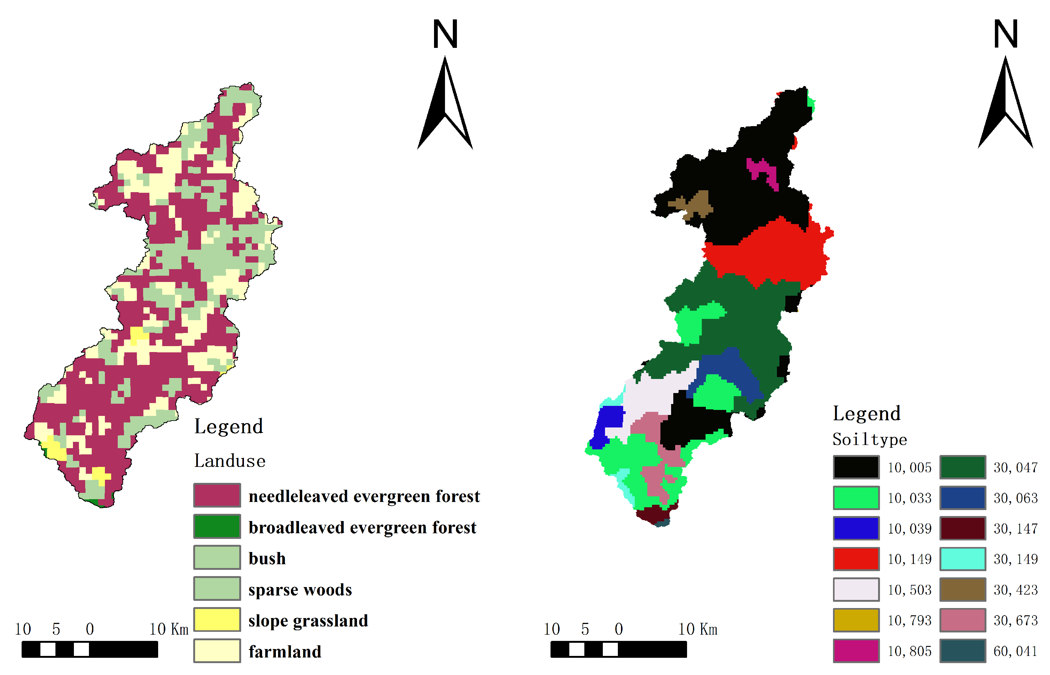
Modeling with the Liuxihe Model requires three types of basic watershed geographic feature data: DEM data, land use type data, and soil type data. The DEM data used in this study is Aster GDEM data, based on which model parameters such as slope and aspect can be calculated, and the watershed boundary can be extracted. The land use type data is derived from the China Land Use Data released by the Joint Research Centre of the European Commission. The soil type data is obtained from the SOTER (Soil and Terrain) China Soil Database; based on this, soil-related parameters in the Liuxihe Model (e.g., soil thickness, saturated soil water content, field capacity) can be calculated using the soil water characteristic calculator proposed by Arya et al. [33]. All three types of data can be downloaded for free from the Internet: DEM data can be downloaded from https://www.gscloud.cn/home (accessed on 6 August 2025). The DEM and hierarchical structure of the watershed rivers are shown in Figure 2.
Land use data can be downloaded from https://forobs.jrc.ec.europa.eu/glc2000 (accessed on 6 August 2025) and soil type data can be downloaded from https://www.fao.org/soils-portal/soil-survey/soil-classification/geology-unified-soil-classification/zh/ (accessed on 6 August 2025) (Figure 3).
Based on previous research results on the impact of the watershed area on the performance of distributed hydrological models, the spatial resolution of the model was set to 90 m; considering the requirements of regional flood control forecasting, the temporal resolution of the model was set to 1 h. In ArcMAP 10.7, the original data was resampled to 90 m, and then the temporal resolution of flood, rainfall, and other data, as well as the model calculation time step, were set to 1 h. Rainfall-flood data are shown in Table 1.

2.4. Overview of the Liuxihe Model

The Liuxihe Model is a physically based distributed hydrological model initially developed for flood forecasting in the Liuxihe Reservoir Watershed [16]. The integrated software system based on the Liuxihe Model (CYB.LMS) has obtained the registration of National Computer Software Copyright of China; on this basis, the Liuxihe Model Flood Forecasting System (CYB.LMS-R) was established for watershed flood forecasting. To date, the Liuxihe Model has been successfully applied in fields such as large-watershed flood forecasting [34], real-time inflow flood forecasting for reservoirs [35], urban waterlogging and flood forecasting [36], and small and medium-sized watershed flood forecasting [37].
As a physically based distributed hydrological model, the Liuxihe Model is structured by dividing the DEM into multiple grid units based on DEM data. Each grid unit has its own attributes, and model parameters represented by each unit can be derived through calculations. These units are classified into three types: reservoir units, slope units, and river channel units. The Liuxihe Model further divides the watershed vertically into canopy, soil layer, and groundwater layer; based on the three unit types (reservoir, slope, and river channel), it calculates evapotranspiration, runoff generation, and confluence to describe the response of flood processes to rainfall. Slope units and river channel units are divided by combining the Strahler method (for river classification) and the D8 flow direction method (for cumulative flow). The river channels in the Hezikou Watershed can be classified into three levels, as shown in Figure 2.
For distributed hydrological models, parameter optimization is required during modeling to improve simulation and forecasting accuracy [38]. Therefore, selecting an appropriate optimization method is also crucial for model establishment. The Liuxihe Model adopts the PSO algorithm [39] for parameter optimization. Since the parameters of the Liuxihe Model are derived from remote sensing data, which inevitably contain errors and uncertainties, the model sets parameters to vary within the range of 0.5–1.5 times their initial values to account for these deviations [34]. Each particle in the PSO algorithm represents a variation coefficient for each model parameter, which moves and changes continuously as the algorithm runs to achieve the optimal solution. Optimized parameters are obtained by multiplying the initial parameters by the scaling coefficient represented by the particles. The model uses Kling–Gupta Efficiency (KGE) [40], Nash–Sutcliffe Efficiency (NSE) [41], Peak Relative Error (PRE), and Absolute Peak Time Error (APTE) to evaluate model performance.

2.5. Rainfall Spatial Interpolation Methods

In the study of flood forecasting using distributed hydrological models, accurately obtaining the spatial distribution of rainfall is crucial, as rainfall is the key piece of input data driving hydrological processes. However, due to the discrete distribution and limited number of rainfall stations in the watershed, spatial interpolation methods are required to convert discrete rainfall station data into continuous areal rainfall data. In this study, the time resolution of rainfall and flood process data is 1 h, which requires interpolation methods to not only process high-frequency data quickly but also reflect the spatial distribution of rainfall relatively accurately within a limited time. Considering the complexity of method principles and applicability in different scenarios, this study selects three methods for rainfall spatial interpolation: THI, IDW, and TSI. Their principles are briefly introduced below.
The Thiessen Polygon Method [42] has a relatively simple principle. Based on the proximity principle, its core idea is to divide the entire study area into multiple polygons, each containing one rainfall station; the rainfall at any point within a polygon is represented by the measured value of the rainfall station in that polygon. For each rainfall station in the study area, its influence range is determined by constructing perpendicular bisectors; these perpendicular bisectors connect to form polygons, i.e., Thiessen polygons.
On the IDW method [43], the nearest several sampling points to the point to be interpolated contribute the most to it, and the contribution is inversely proportional to the distance. This relationship is described by weights in the method. Its formula is as follows:
Z = i = 1 n   Z i D i P i = 1 n   D i P
In the formula, Z   is the interpolation result, Z i is the measured value of the i-th rainfall station,   D is the distance, and P is the distance power, which significantly affects the interpolation result. The selection criterion for P is the minimum mean absolute error. Here, P is set to 2, i.e., the inverse distance squared weighting method.
The TSI method adopts a global polynomial regression approach. It can be used to describe long-distance gradual features: by fitting a smooth surface defined by a mathematical function to the output sampling points, a smooth surface reflecting the gradual trend of the study area’s surface is obtained. The more complex the polynomial used, the more complex the physical meaning it endows [44]. Its formula is as follows:
Y = F θ 1 φ + e
In the formula, Y is the measured rainfall value, F θ 1 φ is the interpolation result, θ is the longitude, φ is the latitude, and F is the trend value affected by macro factors (longitude and latitude); e is the difference between the measured value and the trend value, which can reflect the influence of local terrain and random errors. When ignoring the influence of small local terrain variations, the formula for the quadratic trend surface is as follows:
F λ 1 φ = b 0 + b 1 θ + b 2 φ + b 3 θ 2 + b 4 θ φ + b 5 φ 2
In the formula, b0b5 are undetermined coefficients.
To explore the response of simulation results to rainfall spatial distribution under different rainfall spatial interpolation methods, this study sets the seven uniformly distributed rainfall stations in the watershed into four scenarios based on their distribution: full coverage (All), upstream-only (Up), downstream-only (Down), and single station (One). These four scenarios represent, respectively, the normal scenario of full coverage of rainfall stations in a region, and scenarios of no rainfall station coverage in the downstream, no coverage in the upstream, and only one rainfall station coverage—all caused by complex natural conditions in the watershed.
In ArcMap 10.7, the watershed terrain, river system, and remote sensing images are overlaid to determine the specific locations of rainfall stations, thereby defining the division of upstream and downstream rainfall stations. This study classifies stations based on terrain and flow direction characteristics: stations located in high-elevation areas (e.g., mountains and hills, with high elevation in DEM images) and in the initial segment along the flow direction are classified as upstream rainfall stations; the opposite are downstream rainfall stations. For the single-station scenario, considering representativeness and applicability, the rainfall station with the highest correlation with the measured data of the other six stations is selected to describe the watershed’s rainfall characteristics. The correlation is quantified using the Pearson correlation coefficient [45]:
r = i = 1 n x i x ¯ y i y ¯ i = 1 n x i x ¯ 2 i = 1 n y i y ¯ 2
In the formula, r 0.8 indicates high correlation; 0.5 r 0.8 indicates moderate correlation; 0.3 r 0.5 indicates low correlation; and r < 0.3 indicates negligible correlation.
The final correlation coefficient calculations are shown in Table 2. As indicated in the table, the mean correlation coefficients between Xinqiao and other rainfall stations are the highest. Therefore, Xinqiao is selected as the representative site for describing the surface rainfall across the entire watershed.

3. Results

3.1. Simulation Results Based on Thiessen Polygon Interpolation

The PSO algorithm was used to optimize the initial model parameters, with the flood event on 10 June 2005 selected as the training sample. First, a model was constructed based on the existing rainfall station distribution scenario in the Hezikou Watershed using the Thiessen Polygon Interpolation method, and parameters were optimized. The optimization results are shown in Figure 4. Figure 4a compares results before and after parameter optimization for the 10 June 2005 flood event. Figure 4b illustrates the parameter optimization process, depicted by changes in the objective function value. After 50 iterations, convergence was achieved around the 20th iteration. Post-optimization improvements include reduced peak discharge error and peak occurrence time, with NSE reaching 0.91 and with peak discharge error reduced to within 20%. This demonstrates the effectiveness of parameter optimization, indicating that the optimized parameters can be used for further model predictions. Subsequently, the optimized parameters were applied to simulate other flood events for validation, yielding the results in Figure 5. Notably, the 4 October 2008 flood event exhibited near-zero flow for the first 20 h due to prolonged drought preceding the flood onset. Table 3 presents the calculated metrics for evaluating model performance. The data indicate that both the NSE and KGE for the model results fluctuate between 0.8 and 0.9, with peak flow errors consistently around 10%.

3.2. Impact of Interpolation Methods on Simulation Results

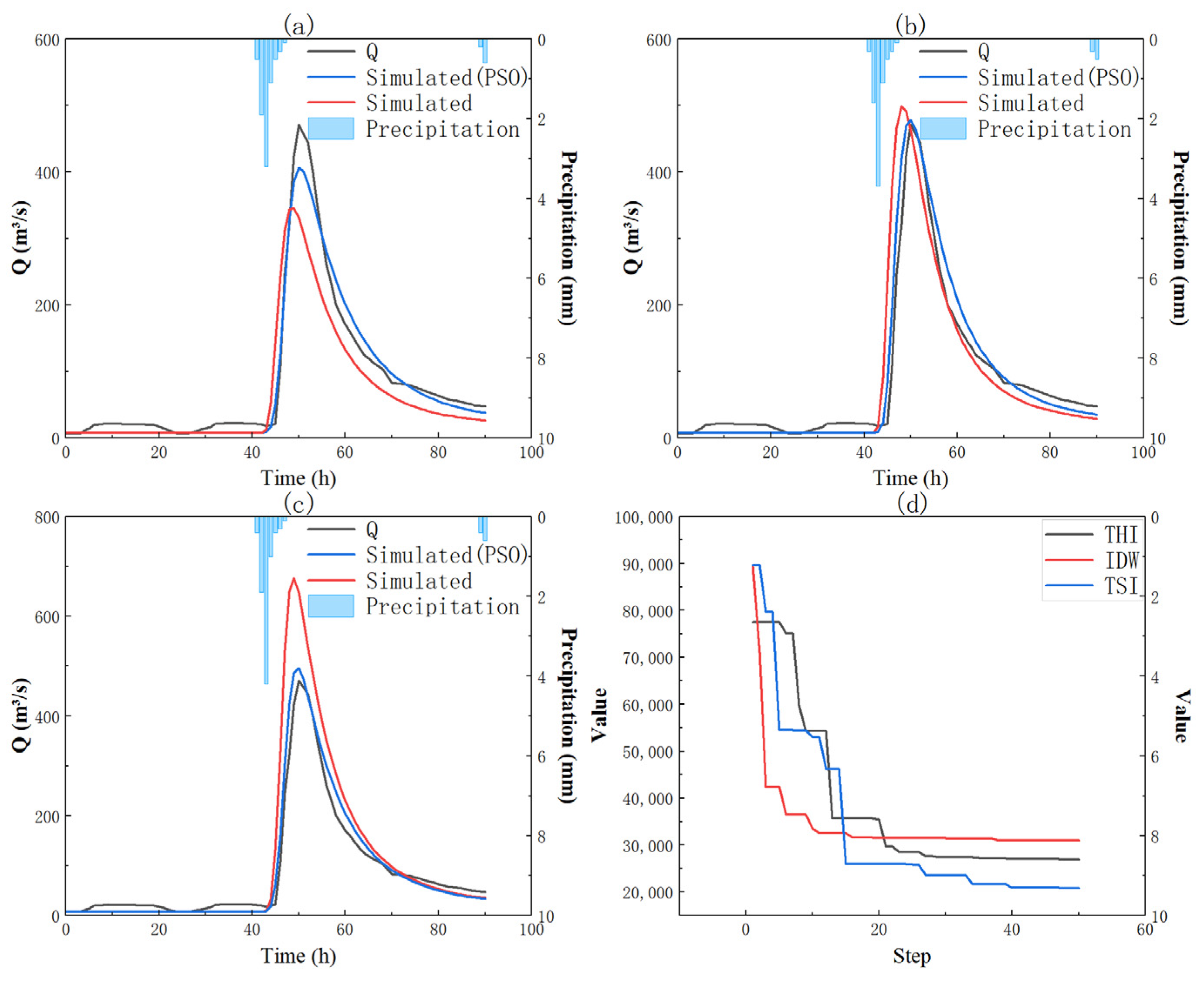
The IDW and TSI methods were introduced, with the 10 June 2005 flood event selected as training data to optimize model parameters in the existing rainfall station distribution scenario in the Hezikou River Basin. The optimization results are shown in Figure 6. Figure 6a–c depict the measured versus predicted flood process curves for the Thiessen polygon method, Inverse Distance Weighting method, and trend surface method, respectively. Figure 6d illustrates the parameter optimization iteration process of the PSO algorithm in the three scenarios, characterized by changes in the objective function value during 50 iterations. THI and IDW converged after approximately 20 iterations, while TSI converged after 40 iterations. Both methods showed improvements in peak flow error and peak occurrence time after optimization. Consequently, the prediction results were enhanced through parameter optimization, with peak flow errors consistently reduced to within 20%.
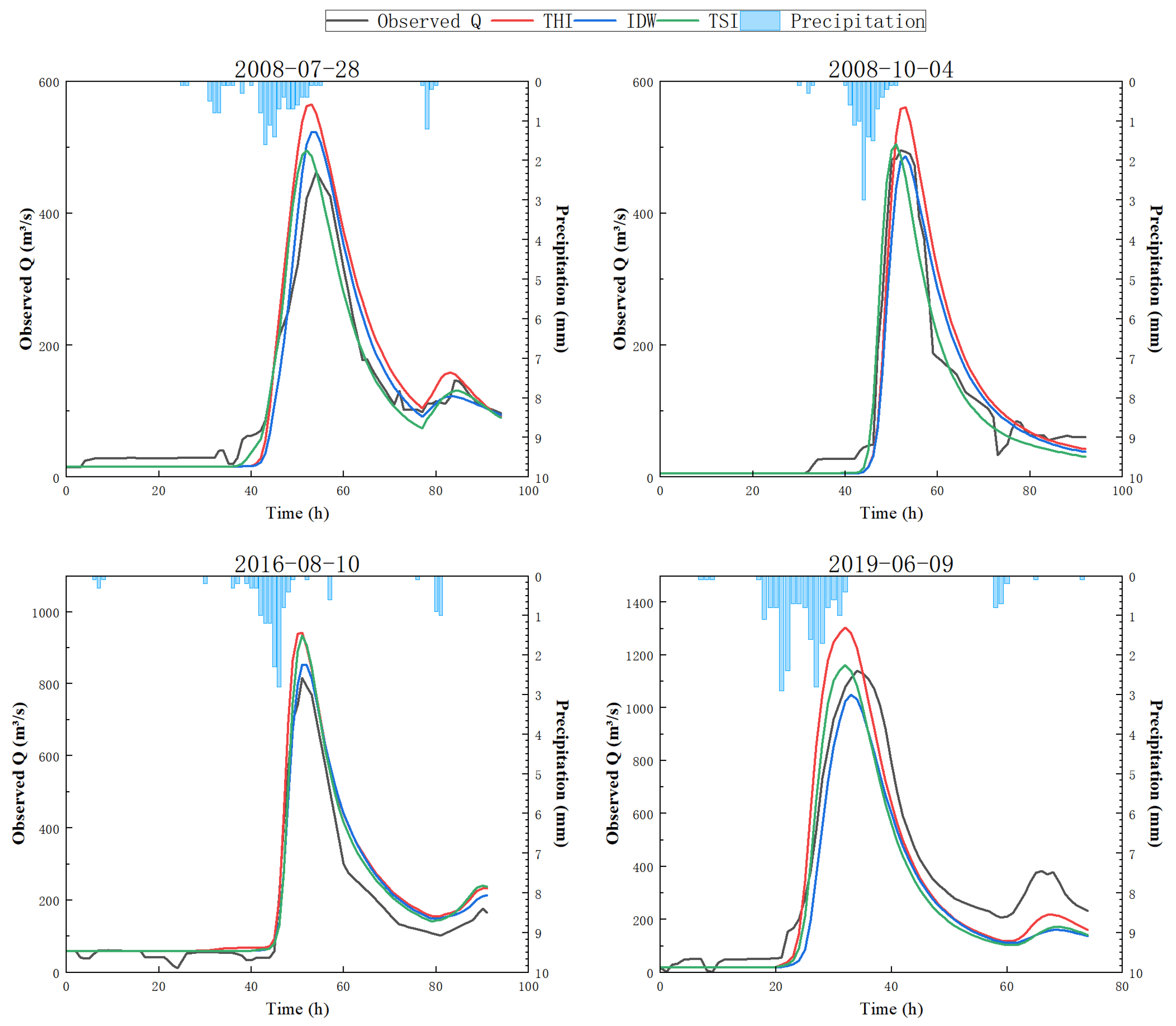
Figure 6 demonstrates that IDW yields significantly superior simulation results compared to the THI method both before and after parameter optimization. The optimized parameters were then applied to other flood events for validation. Figure 7 presents flood simulation curves for four test events using the three interpolation methods. The figures reveal that all three interpolation methods demonstrate certain forecasting capabilities. However, the THI method yields poorer prediction results compared to IDW and TSI, with overall peak discharge errors higher than the other two methods. IDW demonstrated the best overall performance. Table 4 presents the calculated metrics for model performance evaluation. The data indicates that IDW achieved an average NSE of 0.9304, representing a 6.9% improvement over THI’s 0.8706. The average KGE was 0.8846, a 7.3% increase compared to THI’s 0.8274. The average relative peak flow error was 5.28%, lower than the 10.8% for THI and 7.06% for TSI. Regarding peak occurrence timing, IDW showed a 1 h error in only one event, while the peak timing errors for the other events were all 0 h.

3.3. Model Performance in Extremely Sparse Rainfall Station Distribution Scenarios

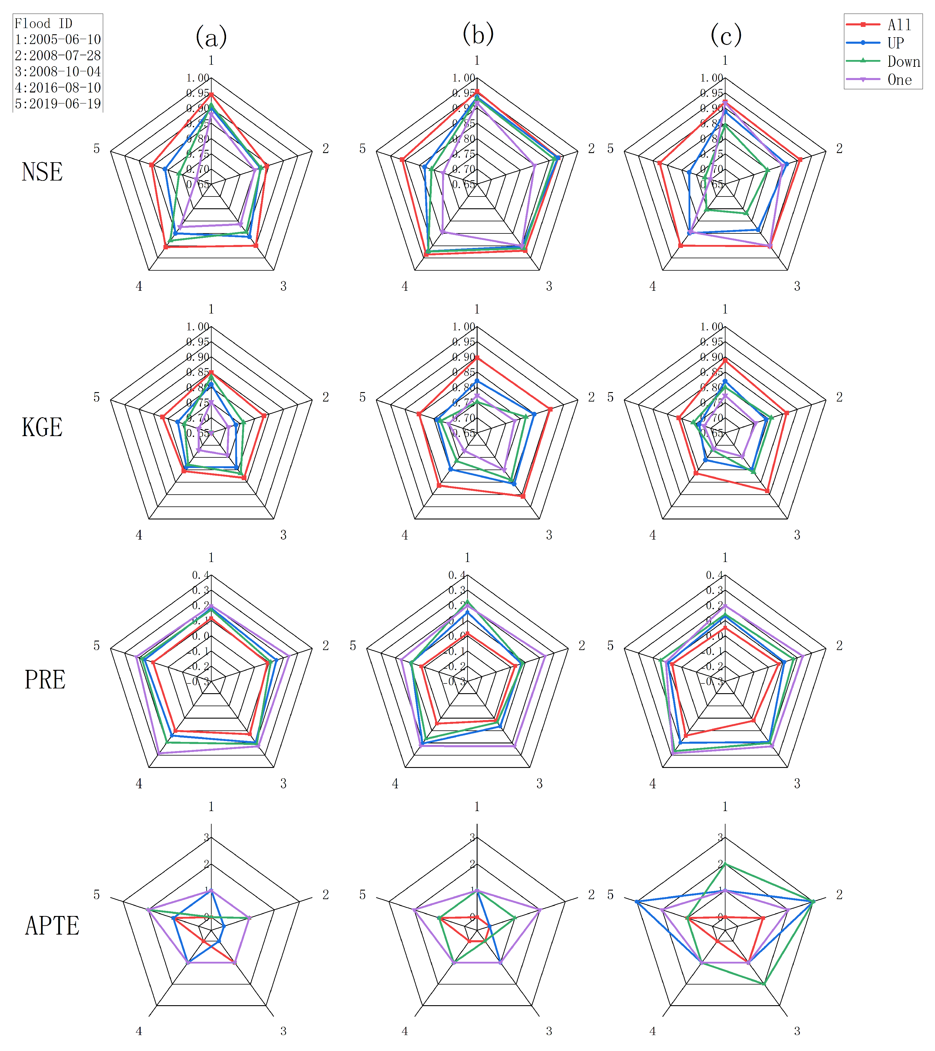
The rainfall stations within the watershed were configured into four scenarios: full coverage (All), upstream only (Up), downstream only (Down), and single rainfall station (One). Simulations were also conducted in the other three scenarios, and the results of the model performance evaluation metrics were calculated (Figure 8). This analysis examined how the simulation results of each interpolation method responded to changes in the spatial distribution of rainfall in scenarios with extremely sparse rainfall stations.
Figure 8 depicts the statistical distributions of the four evaluation metrics NSE, KGE, PRE, and APTE across four scenario simulations. Figure 8a–c represent the results of the THI, IDW, and TSI methods, respectively. The four scenarios—All, Up, Down, and One—are color-coded as red, blue, green, and purple, respectively. In the radar chart, axes 1, 2, 3, 4, and 5 correspond to the five flood events on 10 June 2005, 28 July 2008, 4 October 2008, 10 August 2016, and 9 June 2019, respectively. The number axes represent the metric values.
Figure 8 reveals that the THI method yields acceptable results for all evaluation indicators when rainfall stations are fully distributed. However, as station density decreases, NSE and KGE significantly contract while PRE and APTE expand. In single-station scenarios, indicators “collapse,” demonstrating extremely poor adaptability to sparse station distributions. The IDW method exhibits stable radar chart patterns across all scenarios. With full rain gauge coverage, its indicators outperform both the THI and TSI methods. In sparse scenarios, NSE and KGE show minimal contraction, while PRE and APTE remain controllable. Leveraging distance weighting, it better accommodates sparse rain gauge distributions, supporting stable model simulations. The TSI method performs similarly to IDW when stations are fully distributed. However, in sparse scenarios (especially single-station scenarios), its metrics rapidly deteriorate. Due to its reliance on fitting global trends, uneven distribution often leads to misjudged trends, reducing model performance.
In summary, THI exhibits poor adaptability to sparse rainfall station distributions, while TSI proves more effective only when stations are uniformly distributed. IDW delivers the most stable and optimal overall performance across all scenarios. This further validates the applicability of the IDW convective stream model for flood forecasting in the Hezikou River Basin.

4. Discussion

4.1. Differences in Spatial Characteristics of Interpolation Results

Figure 9 shows the interpolation results of the three methods in various scenarios (taking the 45th-hour rainfall process of the 10 June 2005 flood event as an example). From Figure 9, the differences in spatial characteristics of the three methods are as follows:
  • THI method: The interpolation results show a discrete polygon block distribution. In sparse rainfall station scenarios, the area of polygons expands, and the boundaries between high-value and low-value areas change abruptly, completely losing the gradual spatial characteristics of rainfall. For example, in the One scenario, the entire watershed is covered by a single rainfall value, which fails to reflect the redistribution effect of mountain and hill terrain on rainfall, leading to significant changes in prediction results.
  • IDW method: The interpolation results show a continuous and smooth spatial gradient. Through the distance-weighting mechanism, even in the One scenario, rainfall information can be reasonably diffused outward from the single rainfall station, resulting in a natural rainfall transition within the watershed. This is more consistent with the spatial distribution pattern of rainfall caused by the Hezikou Watershed’s terrain (higher in the southwest and lower in the northeast), ensuring the stability and prediction accuracy of the Liuxihe Model in this watershed.
  • TSI method: The interpolation results rely on global trend fitting. In the All scenario, the trend surface can well fit multi-station data; however, in the Up or Down scenarios, the trend surface is overly biased toward the area with concentrated stations. For example, in the Up scenario, rainfall in the upstream is overestimated and that which is in the downstream is underestimated, forming a “false gradient” unrelated to the actual terrain. This leads to deviations in the calculation of the model’s confluence process and significant changes in prediction results.

4.2. Response Law of Model Performance

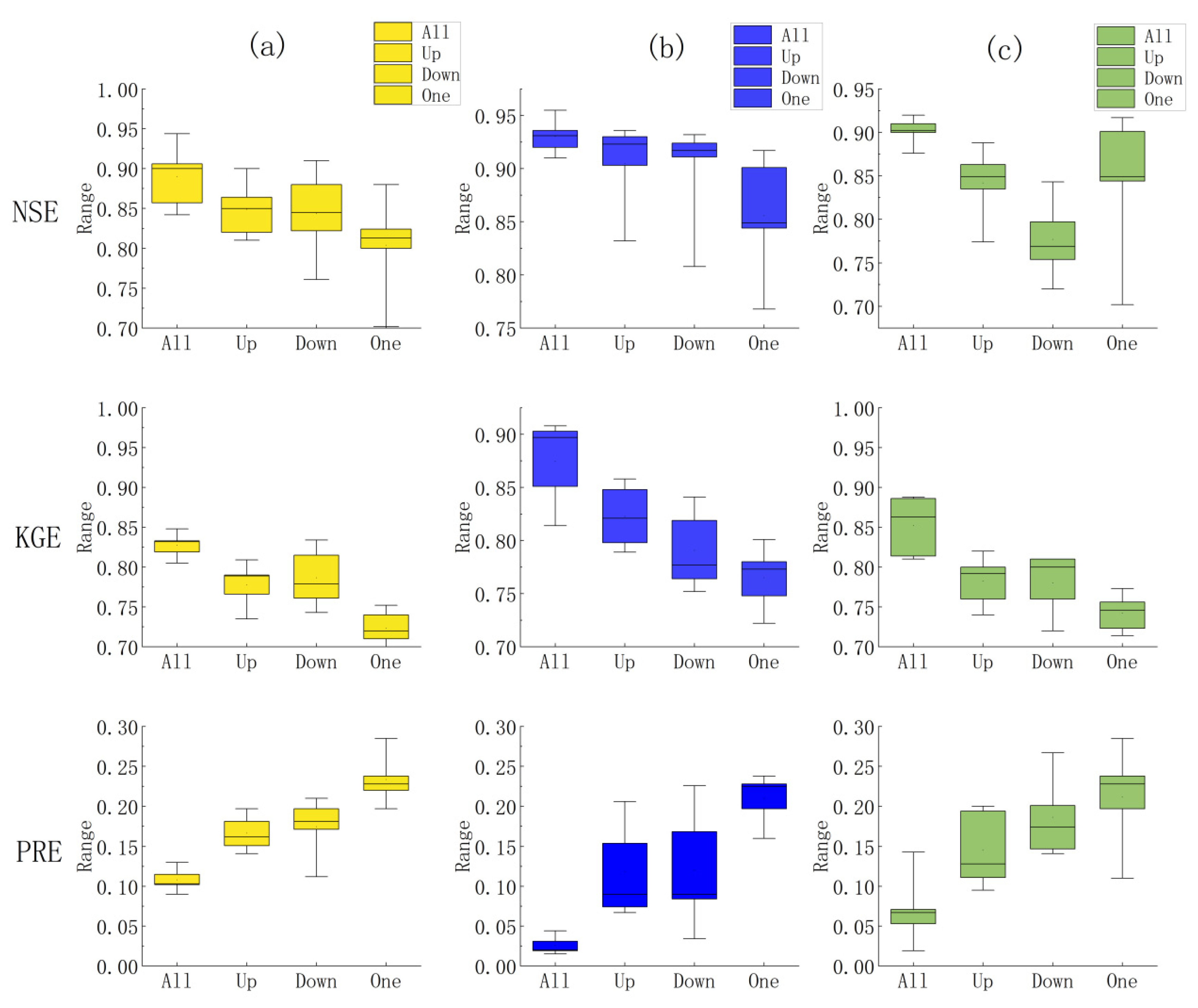
Figure 10 (boxplots) quantifies the performance differences in the three interpolation methods in different scenarios. From Figure 10, the response laws of the three methods are as follows:
  • THI method: As the number of rainfall stations decreases, the NSE and KGE boxes shift downward rapidly (the median NSE drops below 0.75 in the One scenario), and the PRE box shifts upward (the median > 0.15), with a significant increase in dispersion. Due to the loss of spatial heterogeneity of rainfall input caused by block interpolation, the model cannot distinguish the runoff generation capacity of different regions, and the flood peak simulation error increases significantly as the number of rainfall stations decreases.
  • IDW method: The NSE and KGE boxes are concentrated and stable in all scenarios (the median NSE remains > 0.85 in the One scenario), and the PRE box is always at a low level (the median < 0.08). The distance-weighting mechanism effectively balances local and global rainfall information; in the single-station scenario, a certain spatial gradient is retained through the distance decay law, making the simulation of the model’s runoff generation and confluence processes more stable and controlling the flood peak error within an acceptable range.
  • TSI method: Its performance is close to that of IDW in the All scenario; however, the boxes change drastically in sparse scenarios (the median KGE drops below 0.7 in the Up scenario). Especially in the One scenario, the extreme value of PRE exceeds 0.3. Single-station data cannot support global trend fitting, leading to significant deviations between the spatial distribution of rainfall and reality, and “trend misjudgment” in the model’s response to flood processes.
In conclusion, in extremely sparse rainfall station network scenarios, the IDW method still shows significant advantages in the Hezikou Watershed—especially in areas with gentle local terrain changes—effectively avoiding the “hole effect.” This further indicates that IDW can be used as the preferred interpolation method for flood simulation and forecasting with the Liuxihe Model in this watershed.
In addition, combining other data sources (e.g., satellite-based rainfall measurement data or meteorological radar data [46,47]) can improve the accuracy of rainfall interpolation in areas with sparse rainfall station networks, thereby enhancing the accuracy of flood forecasting. Finally, climate change may alter rainfall patterns; therefore, further research on the combined impact of interpolation methods and rainfall station networks on flood forecasting in climate change scenarios is also of great importance [48,49,50].
To further validate the reliability of our findings, we contextualize them with existing research on rainfall interpolation methods. Zimmerman et al. [32] conducted a comparative experiment on Kriging and IDW and found that IDW exhibits more stable performance in sparse data scenarios due to its independence from spatial correlation assumptions—this aligns with our conclusion that IDW outperforms THI and TSI under extremely sparse station conditions (e.g., single-station scenario, NSE > 0.85). Gilewski [29] emphasized that the adaptability of interpolation methods is closely tied to station distribution uniformity, and our study supplements this insight by quantifying performance differences across four typical scenarios (full coverage, upstream-only, downstream-only, single-station): we found that IDW’s performance decline (NSE reduction of only 3%) is far smaller than THI (18%) and TSI (12%), which further confirms IDW’s robustness in unevenly distributed stations. Additionally, Helmi et al. [22] noted that IDW’s distance-weighting mechanism can generate continuous rainfall gradients consistent with terrain, and our results specifically verify this in the Hezikou Watershed—IDW’s interpolation results match the basin’s “southwest high–northeast low” terrain-driven rainfall pattern, while THI’s discrete polygons and TSI’s false gradients fail to do so. These consistencies with prior studies confirm the generalizability of our findings, while our scenario-based analysis enriches the understanding of interpolation methods in small and medium-sized sparsely gauged basins.
While our results provide valuable insights for flood forecasting, this study also has several limitations that should be acknowledged to guide future research. First, the IDW method’s performance in this study depends on the distance power parameter P (set to 2 based on minimum mean absolute error), but different P values may affect interpolation accuracy in basins with more complex terrain (e.g., high-altitude mountainous basins with dramatic elevation changes)—this parameter sensitivity requires further exploration. Second, TSI’s poor performance in sparse scenarios could potentially be improved by integrating terrain factors (e.g., elevation, slope) into the global trend fitting (rather than only using longitude and latitude), which was not tested in our current design. Third, our study focuses on the humid/semi-humid Hezikou Watershed, and the applicability of IDW in arid/semi-arid regions—where rainfall is more spatially variable and extreme—remains unvalidated. Addressing these limitations will help expand the practical value of the proposed interpolation scheme.

5. Conclusions

Taking the Hezikou Watershed as the study area, this study focuses on the applicability of rainfall interpolation methods for the Liuxihe Model in flood forecasting of this watershed. It introduces the Inverse Distance Weighting (IDW) method and Trend Surface Interpolation (TSI) method, and conducts flood forecasting research using the Liuxihe Model in combination with the model’s original Thiessen Polygon Method (THI). It further analyzes the response of simulation results of different interpolation methods to changes in rainfall spatial distribution in extremely sparse rainfall station scenarios. The main conclusions are as follows:
  • The original Thiessen Polygon Method (THI) of the Liuxihe Model has limitations in watersheds with sparse rainfall stations. Based on the proximity principle, THI divides the watershed into discrete polygons. In the Hezikou Watershed with sparse rainfall stations (only seven stations, i.e., one station per 150 km2), the model prediction results are poor. Moreover, as the number of rainfall stations decreases and their distribution becomes uneven, the interpolation results lose a large amount of spatial heterogeneity information about rainfall; the abrupt rainfall changes at polygon boundaries are inconsistent with the actual gradual rainfall characteristics. In the upstream-only, downstream-only, and especially single-station scenarios, model performance deteriorates sharply: NSE and KGE values decrease significantly, while PRE and APTE increase significantly, failing to meet the accuracy requirements for flood forecasting.
  • Comparing the Inverse Distance Weighting (IDW) method and Trend Surface Interpolation (TSI) method, IDW shows the best adaptability and stability in the Hezikou Watershed. Through the distance-weighting mechanism, IDW integrates the influence of surrounding rainfall stations, and its interpolation results show a continuous and smooth spatial gradient—more consistent with the rainfall distribution pattern caused by the watershed’s terrain. In different rainfall station distribution scenarios, model performance remains stable; even in the single-station scenario, NSE can still be maintained above 0.85, KGE around 0.78, and PRE only 0.09—reducing the error by more than 50% compared with THI. This can effectively support the Liuxihe Model in accurate flood forecasting, especially suitable for scenarios with sparse rainfall stations.
In summary, in regions with humid to semi-humid climates and sparse rainfall stations, such as the Hezikou River basin, the Inverse Distance Weighting (IDW) method demonstrates greater effectiveness than the Thiessen polygon (THI) and Trend Surface Interpolation (TSI) methods in enhancing the flood forecasting accuracy of the Liu Xi River model. This finding provides scientific reference for selecting flood forecasting interpolation methods in similar basins.

Author Contributions

Conceptualization, Y.C. and D.F.; methodology, D.F.; validation, D.F. and P.J.; formal analysis, D.F.; investigation, D.F.; resources, D.F. and P.J.; data curation, D.F. and J.N.; writing—original draft preparation, D.F.; writing—review and editing, Y.C.; visualization, D.F.; supervision, Y.C.; project administration, Y.C.; funding acquisition, Y.C. All authors have read and agreed to the published version of the manuscript.

Funding

This research was funded by the Open Research Fund of Anhui Provincial Key Laboratory of Water Conservancy and Water Resources (Grant No. 2023SKJ04) and the Natural Science Foundation of China (Grant No. U2243227).

Data Availability Statement

Hydrological data are unavailable due to privacy. Remote sensing data can be downloaded online.

Conflicts of Interest

The authors declare no conflicts of interest. The funders had no role in the design of the study; in the collection, analyses, or interpretation of data; in the writing of the manuscript; or in the decision to publish the results.

Abbreviations

The following abbreviations are used in this manuscript:
THIThiessen Polygon Interpolation
TSITrend Surface Interpolation
IDWInverse Distance Weighting
NSENash–Sutcliffe Efficiency
KGEKling–Gupta Efficiency
PREPeak Relative Error
PBDHMPhysically Based Distributed Hydrological Model
GISGeographic Information System
DEMDigital Elevation Model
PSOParticle Swarm Optimization
APTEAbsolute Peak Time Error
SOTERSoil and Terrain

References

  1. Liu, Z.; Guo, S.; Zhang, H.; Liu, D.; Yang, G. Comparative Study of Three Updating Procedures for Real-Time Flood Forecasting. Water Resour. Manag. 2016, 30, 2111–2126. [Google Scholar] [CrossRef]
  2. Xie, A.; Liu, P.; Guo, S.; Zhang, X.; Jiang, H.; Yang, G. Optimal Design of Seasonal Flood Limited Water Levels by Jointing Operation of the Reservoir and Floodplains. Water Resour. Manag. 2018, 32, 179–193. [Google Scholar] [CrossRef]
  3. Thiboult, A.; Anctil, F. On the difficulty to optimally implement the Ensemble Kalman filter: An experiment based on many hydrological models and catchments. J. Hydrol. 2015, 529, 1147–1160. [Google Scholar] [CrossRef]
  4. Jie, M.-X.; Chen, H.; Xu, C.-Y.; Zeng, Q.; Tao, X.-E. A comparative study of different objective functions to improve the flood forecasting accuracy. Hydrol. Res. 2015, 47, 718–735. [Google Scholar] [CrossRef]
  5. Su, B.; Huang, H.; Zhu, W. An urban pluvial flood simulation model based on diffusive wave approximation of shallow water equations. Hydrol. Res. 2017, 50, 138–154. [Google Scholar] [CrossRef]
  6. Huang, S.; Hattermann, F.F. Coupling a global hydrodynamic algorithm and a regional hydrological model for large-scale flood inundation simulations. Hydrol. Res. 2017, 49, 438–449. [Google Scholar] [CrossRef]
  7. Todini, E. The ARNO rainfall—Runoff model. J. Hydrol. 1996, 175, 339–382. [Google Scholar] [CrossRef]
  8. Duan, W.; Guo, S.; Wang, J.; Liu, D. Impact of Cascaded Reservoirs Group on Flow Regime in the Middle and Lower Reaches of the Yangtze River. Water 2016, 8, 218. [Google Scholar] [CrossRef]
  9. Lin, K.; Zhang, Q.; Chen, X. An evaluation of impacts of DEM resolution and parameter correlation on TOPMODEL modeling uncertainty. J. Hydrol. 2010, 394, 370–383. [Google Scholar] [CrossRef]
  10. Graf, W.L. Downstream hydrologic and geomorphic effects of large dams on American rivers. Geomorphology 2006, 79, 336–360. [Google Scholar] [CrossRef]
  11. Kapangaziwiri, E.; Hughes, D.A.; Wagener, T. Incorporating uncertainty in hydrological predictions for gauged and ungauged basins in southern Africa. Hydrol. Sci. J. 2012, 57, 1000–1019. [Google Scholar] [CrossRef]
  12. Worqlul, A.W.; Yen, H.; Collick, A.S.; Tilahun, S.A.; Langan, S.; Steenhuis, T.S. Evaluation of CFSR, TMPA 3B42 and ground-based rainfall data as input for hydrological models, in data-scarce regions: The upper Blue Nile Basin, Ethiopia. CATENA 2017, 152, 242–251. [Google Scholar] [CrossRef]
  13. Freeze, R.A.; Harlan, R.L. Blueprint for a physically-based, digitally-simulated hydrologic response model. J. Hydrol. 1969, 9, 237–258. [Google Scholar] [CrossRef]
  14. Abbott, M.B.; Bathurst, J.C.; Cunge, J.A.; O’Connell, P.E.; Rasmussen, J. An introduction to the European Hydrological System—Systeme Hydrologique Europeen, “SHE”, 1: History and philosophy of a physically-based, distributed modelling system. J. Hydrol. 1986, 87, 45–59. [Google Scholar] [CrossRef]
  15. Wang, Z.-M.; Batelaan, O.; De Smedt, F. A distributed model for water and energy transfer between soil, plants and atmosphere (WetSpa). Phys. Chem. Earth 1996, 21, 189–193. [Google Scholar] [CrossRef]
  16. Chen, Y.; Ren, Q.; Huang, F.; Xu, H.; Cluckie, I. Liuxihe Model and Its Modeling to River Basin Flood. J. Hydrol. Eng. 2011, 16, 33–50. [Google Scholar] [CrossRef]
  17. Julien, P.Y.; Saghafian, B.; Ogden, F.L. Raster-Based Hydrologic Modeling of Spatially-Varied Surface Runoff. J. Am. Water Resour. Assoc. 1995, 31, 523–536. [Google Scholar] [CrossRef]
  18. Liang, X.; Lettenmaier, D.P.; Wood, E.F.; Burges, S.J. A simple hydrologically based model of land surface water and energy fluxes for general circulation models. J. Geophys. Res. Atmos. 1994, 99, 14415–14428. [Google Scholar] [CrossRef]
  19. Ma, L.; He, C.; Bian, H.; Sheng, L. MIKE SHE modeling of ecohydrological processes: Merits, applications, and challenges. Ecol. Eng. 2016, 96, 137–149. [Google Scholar] [CrossRef]
  20. Di Curzio, D.; Di Giovanni, A.; Lidori, R.; Montopoli, M.; Rusi, S. Comparing Rain Gauge and Weather RaDAR Data in the Estimation of the Pluviometric Inflow from the Apennine Ridge to the Adriatic Coast (Abruzzo Region, Central Italy). Hydrology 2022, 9, 225. [Google Scholar] [CrossRef]
  21. Erxleben, J.; Elder, K.; Davis, R. Comparison of spatial interpolation methods for estimating snow distribution in the Colorado Rocky Mountains. Hydrol. Process. 2002, 16, 3627–3649. [Google Scholar] [CrossRef]
  22. Helmi, A.M.; Elgamal, M.; Farouk, M.I.; Abdelhamed, M.S.; Essawy, B.T. Evaluation of Geospatial Interpolation Techniques for Enhancing Spatiotemporal Rainfall Distribution and Filling Data Gaps in Asir Region, Saudi Arabia. Sustainability 2023, 15, 14028. [Google Scholar] [CrossRef]
  23. Maier, R.; Krebs, G.; Pichler, M.; Muschalla, D.; Gruber, G. Spatial Rainfall Variability in Urban Environments—High-Density Precipitation Measurements on a City-Scale. Water 2020, 12, 1157. [Google Scholar] [CrossRef]
  24. Saavedra, O.; Ureña, J.; Perales, M. Implementation of HydroBID Model with Satellite-Based Precipitation Products in Guadalquivir Basin, Bolivia. Water 2023, 15, 3250. [Google Scholar] [CrossRef]
  25. Zare, M.; Schumann, G.J.-P.; Teferle, F.N.; Mansorian, R. Generating Flood Hazard Maps Based on an Innovative Spatial Interpolation Methodology for Precipitation. Atmosphere 2021, 12, 1336. [Google Scholar] [CrossRef]
  26. De Vera, A.; Alfaro, P.; Terra, R. Operational Implementation of Satellite-Rain Gauge Data Merging for Hydrological Modeling. Water 2021, 13, 533. [Google Scholar] [CrossRef]
  27. Fiedler, F.R. Simple, practical method for determining station weights using Thiessen polygons and isohyetal maps. J. Hydrol. Eng. 2003, 8, 219–221. [Google Scholar] [CrossRef]
  28. Pakoksung, K. Impact of Spatial Rainfall Scenarios on River Basin Runoff Simulation a Nan River Basin Study Using the Rainfall-Runoff-Inundation Model. Eng 2024, 5, 51–69. [Google Scholar] [CrossRef]
  29. Gilewski, P. Impact of the Grid Resolution and Deterministic Interpolation of Precipitation on Rainfall-Runoff Modeling in a Sparsely Gauged Mountainous Catchment. Water 2021, 13, 230. [Google Scholar] [CrossRef]
  30. Helmi, A.M.; Farouk, M.I.; Hassan, R.; Mumtaz, M.A.; Chaouachi, L.; Elgamal, M.H. Comparing Remote Sensing and Geostatistical Techniques in Filling Gaps in Rain Gauge Records and Generating Multi-Return Period Isohyetal Maps in Arid Regions—Case Study: Kingdom of Saudi Arabia. Water 2024, 16, 925. [Google Scholar] [CrossRef]
  31. Sucozhañay, A.; Célleri, R. Impact of Rain Gauges Distribution on the Runoff Simulation of a Small Mountain Catchment in Southern Ecuador. Water 2018, 10, 1169. [Google Scholar] [CrossRef]
  32. Zimmerman, D.; Pavlik, C.; Ruggles, A.; Armstrong, M.P. An Experimental Comparison of Ordinary and Universal Kriging and Inverse Distance Weighting. Math. Geol. 1999, 31, 375–390. [Google Scholar] [CrossRef]
  33. Arya, L.M.; Paris, J.F. A Physicoempirical Model to Predict the Soil Moisture Characteristic from Particle-Size Distribution and Bulk Density Data. Soil Sci. Soc. Am. J. 1981, 45, 1023–1030. [Google Scholar] [CrossRef]
  34. Chen, Y.; Li, J.; Wang, H.; Qin, J.; Dong, L. Large-watershed flood forecasting with high-resolution distributed hydrological model. Hydrol. Earth Syst. Sci. 2017, 21, 735–749. [Google Scholar] [CrossRef]
  35. Xing, L.; Chen, Y.; Feng, Y.; Huang, X.; Huang, Z. Research on Flood Forecasting Model for Xinfengjiang Reservoir Based on Liuxihe Model. J. China Hydrol. 2022, 42, 47–53. [Google Scholar] [CrossRef]
  36. Gu, Y.; Chen, Y.; Sun, H.; Liu, J. Remote Sensing-Supported Flood Forecasting of Urbanized Watersheds—A Case Study in Southern China. Remote Sens. 2022, 14, 6129. [Google Scholar] [CrossRef]
  37. Li, J.; Chen, Y.; Zhu, Y.; Liu, J. Study of Flood Simulation in Small and Medium-Sized Basins Based on the Liuxihe Model. Sustainability 2023, 15, 11225. [Google Scholar] [CrossRef]
  38. Chen, Y.; Li, J.; Xu, H. Improving flood forecasting capability of physically based distributed hydrological models by parameter optimization. Hydrol. Earth Syst. Sci. 2016, 20, 375–392. [Google Scholar] [CrossRef]
  39. Kennedy, J.; Eberhart, R. Particle swarm optimization. In Proceedings of the International Conference on Neural Networks (ICNN’95), Perth, WA, Australia, 27 November–1 December 1995; Volume 1944, pp. 1942–1948. [Google Scholar]
  40. Vrugt, J.A.; de Oliveira, D.Y. Confidence intervals of the Kling-Gupta efficiency. J. Hydrol. 2022, 612, 127968. [Google Scholar] [CrossRef]
  41. Nash, J.E.; Sutcliffe, J.V. River flow forecasting through conceptual models part I—A discussion of principles. J. Hydrol. 1970, 10, 282–290. [Google Scholar] [CrossRef]
  42. Tabios, G.Q., III; Salas, J.D. A Comparative Analysis of Techniques for Spatial Interpolation of Precipitation. J. Am. Water Resour. Assoc. 1985, 21, 365–380. [Google Scholar] [CrossRef]
  43. Lu, G.Y.; Wong, D.W. An adaptive inverse-distance weighting spatial interpolation technique. Comput. Geosci. 2008, 34, 1044–1055. [Google Scholar] [CrossRef]
  44. Agterberg, F.P. Trend Surface Analysis. In Spatial Statistics and Models; Gaile, G.L., Willmott, C.J., Eds.; Springer: Dordrecht, The Netherlands, 1984; pp. 147–171. [Google Scholar]
  45. Jian, Y.; Pu, S.; Zhu, J.; Zhang, J.; Xing, W. Estimation of Sow Backfat Thickness Based on Machine Vision. Animals 2024, 14, 3520. [Google Scholar] [CrossRef] [PubMed]
  46. Li, J.; Chen, Y.; Wang, H.; Qin, J.; Li, J.; Chiao, S. Extending flood forecasting lead time in a large watershed by coupling WRF QPF with a distributed hydrological model. Hydrol. Earth Syst. Sci. 2017, 21, 1279–1294. [Google Scholar] [CrossRef]
  47. Yoon, S.-S.; Lee, B. Effects of Using High-Density Rain Gauge Networks and Weather Radar Data on Urban Hydrological Analyses. Water 2017, 9, 931. [Google Scholar] [CrossRef]
  48. AlZaatiti, F.; Halwani, J.; Soliman, M.R. Climate change impacts on flood risks in the Abou Ali River Basin, Lebanon: A hydrological modeling approach. Results Eng. 2025, 25, 104186. [Google Scholar] [CrossRef]
  49. Nurbatsina, A.; Salavatova, Z.; Tursunova, A.; Didovets, I.; Huthoff, F.; Rodrigo-Clavero, M.-E.; Rodrigo-Ilarri, J. Flood Modelling of the Zhabay River Basin Under Climate Change Conditions. Hydrology 2025, 12, 35. [Google Scholar] [CrossRef]
  50. Yang, R.; Xing, B. A Comparison of the Performance of Different Interpolation Methods in Replicating Rainfall Magnitudes under Different Climatic Conditions in Chongqing Province (China). Atmosphere 2021, 12, 1318. [Google Scholar] [CrossRef]
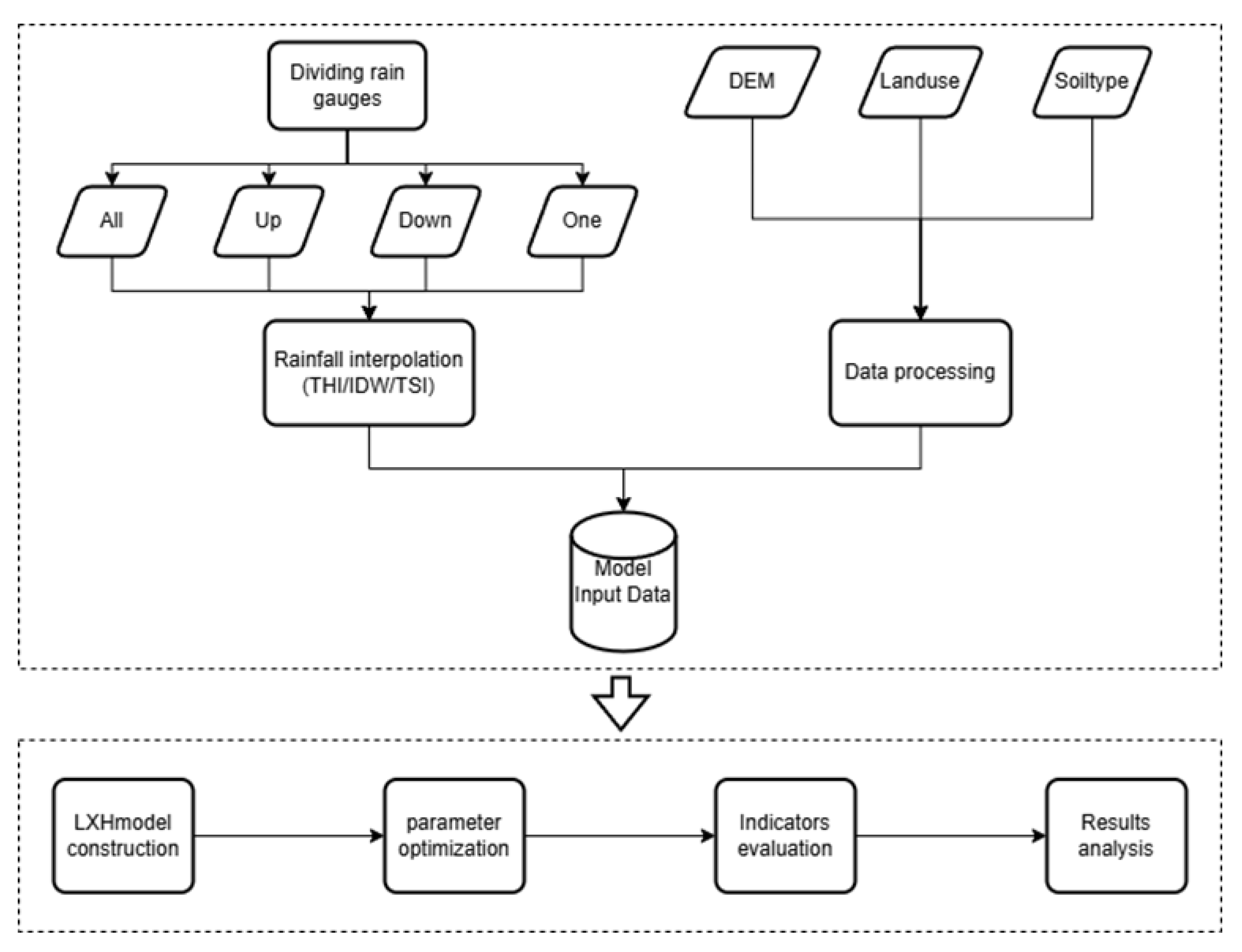
Figure 1. Technical flowchart.
Water 17 03237 g001
Figure 2. Digital elevation map of the Hezikou Watershed and geographic distribution of rainfall stations and channel nodes. The illustration on the left shows the geographical location of the watershed in China and Guangdong Province.
Water 17 03237 g002
Figure 3. Land use data (left) and soil type data (right).
Water 17 03237 g003
Figure 4. Results of model parameter optimization based on THI. (a) Comparison of results before and after parameter optimization; (b) evolution of the parameter optimization objective function.
Water 17 03237 g004
Figure 5. Results of the other four flood simulations (THI method).
Water 17 03237 g005
Figure 6. The curves of flow prediction results and the variation processes of the objective function for three rainfall interpolation methods (10 June 2005 event). (a) THI result curve; (b) IDW result curve; (c) TSI result curve; (d) objective function variation curves for each method.
Water 17 03237 g006
Figure 7. Curves of flow prediction results for each method in the other four flood events.
Water 17 03237 g007
Figure 8. Statistical graph of model prediction evaluation indicators in different rain gauge distribution scenarios. (a) THI result; (b) IDW result; (c) TSI result.
Water 17 03237 g008
Figure 9. Interpolation result of three methods. (a) THI result; (b) IDW result; (c) TSI result.
Water 17 03237 g009
Figure 10. Boxplots of model evaluation indicators for three interpolation methods. (a) THI Result; (b) IDW Result; (c) TSI Result.
Water 17 03237 g010
Table 1. Flood events overview.
Event IdentifierBegin TimeDuration (h)Peak (m3/s)
10 June 200508:00:0091471
28 July 200808:00:0095463
4 October 200810:00:0093496
10 August 201608:00:0092817
9 June 201906:00:00751140
Table 2. Average correlation coefficients for rainfall stations.
Flood IdentifierJionglongLongmuGuqianHuangwupingHeshiWuhuaXinqiao
10 June 20050.441 0.484 0.617 0.373 0.590 0.622 0.771
28 July 20080.472 0.459 0.523 0.373 0.489 0.507 0.779
4 October 20080.824 0.780 0.795 0.671 0.651 0.861 0.868
10 August 20160.411 0.642 0.690 0.448 0.648 0.664 0.733
9 June 20190.546 0.549 0.662 0.551 0.688 0.630 0.818
Table 3. Statistical indicators of simulation results based on THI.
Flood IdentifierNSEKGERPREAPTE (h)
10 June 20050.910.8480.9890.1150
28 July 20080.8420.8320.9820.091
4 October 20080.870.8330.9830.131
10 August 20160.890.8050.9810.1020
9 June 20190.8410.8190.9770.1031
Table 4. Statistical table of evaluation indicators for model prediction results.
Interpolation MethodFlood IdentifierNSEKGERPREAPTE (h)
THI10 June 20050.910.8480.9890.1150
28 July 20080.8420.8320.9820.091
4 October 20080.870.8330.9830.131
10 August 20160.890.8050.9810.1020
9 June 20190.8410.8190.9770.1031
IDW10 June 20050.9550.8970.9880.0350
28 July 20080.9310.9030.9870.0510
4 October 20080.920.9080.960.0540
10 August 20160.9360.8640.9820.0740
9 June 20190.910.8510.9770.051
TSI10 June 20050.920.8880.9910.0530
28 July 20080.910.8630.9750.0711
4 October 20080.9020.8860.9810.0811
10 August 20160.90.8140.9870.1430
9 June 20190.8760.810.9540.0671
Disclaimer/Publisher’s Note: The statements, opinions and data contained in all publications are solely those of the individual author(s) and contributor(s) and not of MDPI and/or the editor(s). MDPI and/or the editor(s) disclaim responsibility for any injury to people or property resulting from any ideas, methods, instructions or products referred to in the content.