Assessing the Applicability of the LTSF Algorithm for Streamflow Time Series Prediction: Case Studies of Dam Basins in South Korea

Abstract

Reliable inflow forecasting represents a challenging and representative problem in long-horizon time series forecasting. Although long-term time series forecasting (LTSF) algorithms have shown strong performance in other domains, their applicability to hydrological inflow prediction has not yet been systematically assessed. Therefore, this study examined two LTSF linear models for inflow forecasting: NLinear and DLinear. LTSF models were trained with a 24 h input window and evaluated for 24 h lead times at eight major dams in South Korea. Long Short-Term Memory (LSTM) network and eXtreme Gradient Boosting (XGBoost) were employed as a conventional AI model. LSTM consistently achieved the highest coefficient of determination (R²) and the lowest normalized root mean square error, DLinear minimized normalized mean square error, and NLinear delivered superior hydrological consistency as measured by Kling–Gupta efficiency. XGBoost showed comparatively larger variability across sites. Spatial heterogeneity was evident; sites were grouped into high-performing, transition, and vulnerable groups. Peak-flow analysis revealed amplitude attenuation and phase lag at longer horizons.

1. Introduction

Climate change has intensified the frequency and severity of floods and droughts, increasing the temporal and spatial variability of dam inflows [1]. Effective reservoir operation—including stable water-level regulation and proactive flood control—therefore requires accurate inflow predictions [2,3]. The reliability of these predictions directly influences the safety margins of release and storage decisions [4,5]. Consequently, developing hourly resolution inflow forecasting systems and rigorously verifying their operational applicability remains a fundamental prerequisite for water resource management [6].

Inflow forecasting has been applied to a wide spectrum of methods over the past several decades. Early studies relied on statistical time-series models such as the autoregressive integrated moving average (ARIMA) and related stochastic approaches [7,8,9,10], which provided a foundation for streamflow prediction but often struggled with non-stationarity and nonlinear catchment behavior [11,12]. With the rise in machine learning, algorithms such as support vector regression (SVR), random forest (RF), and gradient boosting (GB) have been introduced [13,14,15,16,17,18]. In parallel, systematic studies have reviewed the development of neural-network methods for water resource prediction and outlined best practices and future directions [19], as well as synthesized flood-focused ML applications [20]. These methods improve nonlinear mapping and feature selection but often require extensive calibration and data preprocessing, which limits scalability and operational adoption [12,20]. Kim et al. [21] investigated the uncertainty in artificial neural networks (ANNs) from training, model structure, and feature selection. They found that the feature selection is the largest source of uncertainty in ANN modeling.

Deep learning has recently become central to hydrological forecasting. The long short-term memory (LSTM) network [22] has been widely adopted for rainfall–runoff and dam inflow prediction because it can capture long-term dependencies [22,23,24,25,26,27]. Numerous studies have shown that LSTM achieves competitive—and often superior—performance compared with process-based hydrological models across diverse basins [22,23,24,25,26,27]. Nonetheless, several limitations remain, including accuracy degradation at longer lead times, high computational costs, and interpretability challenges, all of which constrain operational deployment [28,29,30].

In parallel, classical statistical forecasting approaches and hybrid data–physics modeling frameworks continue to play an important role in hydrological prediction. For instance, Giorgio et al. [31] demonstrated that the SARIMAX and Holt–Winters models can effectively predict hydrological variables in reclaimed water irrigation systems, emphasizing the practical value of interpretable and computationally lightweight statistical time-series models. Likewise, Gegenleithner et al. [32] showed that integrating LSTM networks with process-based hydrologic models can enhance real-time flood forecasting capability, illustrating the growing interest in hybrid modeling strategies that combine physical process understanding with data-driven learning. These studies indicate that both statistical and hybrid modeling frameworks remain relevant benchmarks for evaluating newer machine learning approaches.

Research on long-term time series forecasting (LTSF) has highlighted the potential of lightweight linear models. Recent studies demonstrated that simple linear mappings on benchmark datasets can match or even outperform transformer-based architectures [33,34]. Two representative variants are NLinear, which applies differencing to stabilize trends before linear regression, and DLinear, which decomposes inputs into trend and residual components prior to modeling [33]. These architectures are computationally efficient, less prone to overfitting, and highly interpretable, making them attractive for operational hydrology where frequent retraining and updates are required [35]. Despite these advantages, LTSF-Linear models are rarely used for dam-inflow forecasting [35]. This gap motivates the present study, which systematically compares LTSF-Linear models (NLinear, DLinear) with LSTM for hourly dam inflow forecasting at eight major reservoirs in South Korea. The objectives are fourfold: (i) quantify each model’s relative strengths using normalized root mean square error (nRMSE), normalized mean absolute error (nMAE), coefficient of determination (R²), mean bias (mBias), and Kling–Gupta efficiency (KGE); (ii) determine maximum reliable lead times for operational use based on threshold criteria; (iii) evaluate site-specific heterogeneity and peak-flow reproduction across lead times; and (iv) identify the best-performing models by lead time and metric. To achieve these goals, we implemented all models within a unified experimental framework, trained them with hourly inflow data from eight representative Korean dams, and evaluated both aggregated and site-specific performance across 24 h prediction horizons.

This study makes three main contributions. First, LTSF-linear models (NLinear, DLinear) are introduced and evaluated for dam inflow forecasting, providing a lightweight alternative to conventional deep-learning architectures. Second, it identifies the maximum reliable forecast horizons and clarifies metric-dependent model strengths, offering operational insights for reservoir management. Third, a multi-metric, site-specific evaluation framework that emphasizes the complementary strengths of linear and nonlinear approaches is established, contributing to more robust hydrological forecasting practice.

2. Materials and Methods

2.1. Study Area and Data

South Korea has a monsoon climate characterized by pronounced seasonal and regional contrasts. The mean annual rainfall is 1252 mm, of which 55.4% (693.9 mm) occurs during the summer monsoon season [36]. Mountainous terrain covers approximately 63% of the land, creating small watersheds and short river lengths that result in rapid runoff and fast discharge to the sea.

These hydrological conditions increase both the variability and seasonality of inflows, complicating prediction and water resource management under high uncertainty. To address these challenges, this study evaluated the applicability of LTSF algorithms for streamflow time series forecasting in South Korea. To avoid the impact of human activity on the streamflow, dam inflow data was used for the streamflow data in the current study. The dams that do not have hydraulic structures in upper basins were considered for the experiment basins.

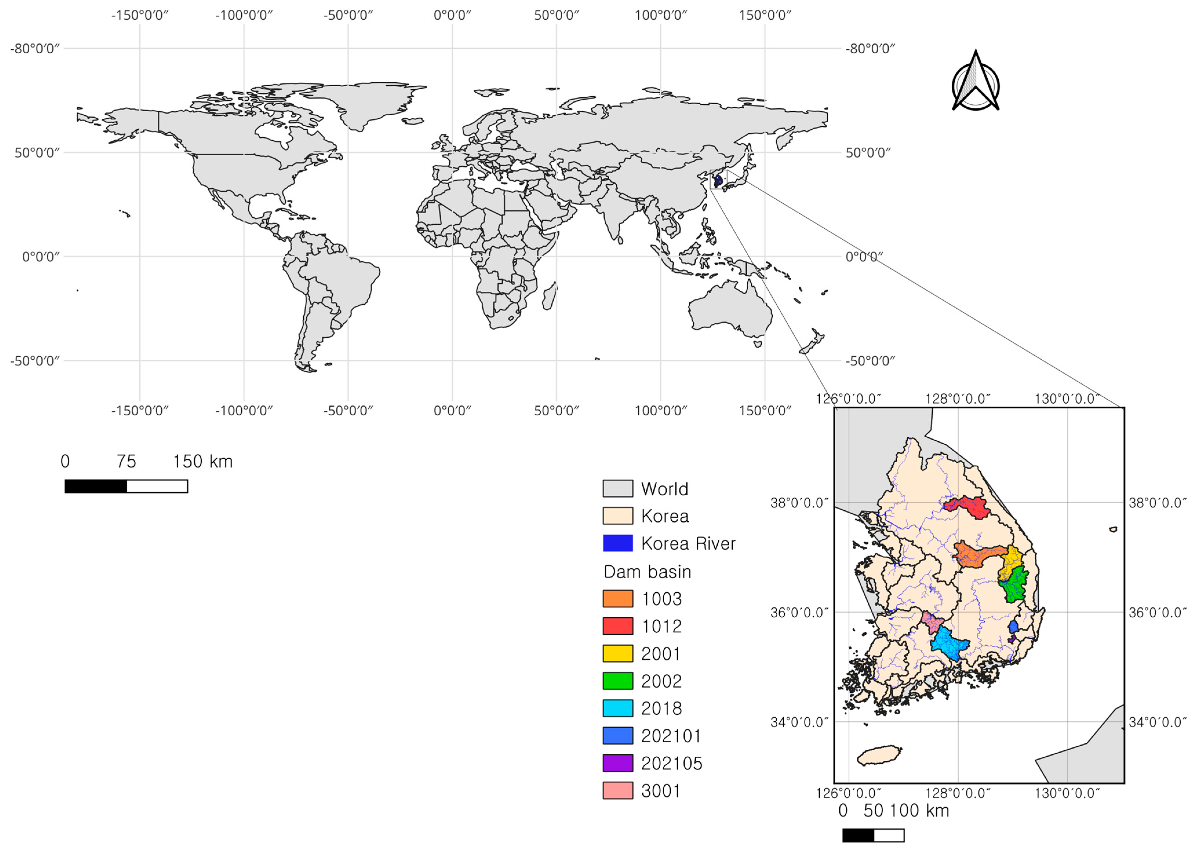
The eight selected dams are located in catchments without upstream dams, ensuring relatively natural hydrological conditions. Their geomorphological and hydrological characteristics—including watershed area, slope, river length, and channel density—along with hourly inflow observations, were obtained from the Water Resources Management Information System (WAMIS) [37]. The diversity of these attributes ensures spatial heterogeneity and hydrological representativeness for model evaluation. Table 1 summarizes key catchment attributes and observation periods for each site, while Figure 1 shows their spatial distribution across South Korea.

Table 1. Catchment characteristics and hydrological properties of the eight dams in this study.

Name	Code	Area (km2)	MeanCatchment Slope (%)	MainStreamLength (km)	Total Stream Length (km)	Drainage Density (km/km2)	Observation Period (YYYYMMDD)	Number of Samples
Andong	2001	1628.7	50.7	170.1	5381.3	3.3	20190212–20241231	51,607
Chungju	1003	2483.8	50.1	115.3	4347.3	1.8	20190208–20241231	51,649
Imha	2002	1975.8	48.7	112.8	5740.9	2.9	20190212–20241231	51,623
Milyang	202105	103.5	54.3	28.1	191.0	1.8	20190212–20241231	51,571
Namgang	2018	2281.7	41.8	110.8	6841.3	3.0	20190212–20241231	51,568
Soyang	1012	1852.0	56.5	156.5	2840.9	1.5	20190208–20241231	51,457
Unmun	202101	302.0	49.4	37.9	674.8	2.2	20190212–20241231	51,600
Yongdam	3001	930.4	42.8	62.6	2130.5	2.3	20190216–20241231	51,457

Figure 1. Geographic distribution of the eight dam catchments in South Korea.

Hourly dam inflow data were obtained from the WAMIS [37], operated by the Ministry of Land, Infrastructure, and Transport, Republic of Korea. The dataset is also available through the United Nations Educational, Scientific and Cultural Organization–International Hydrological Programme repository, “South Korea Hydrometeorological Data from WAMIS” [38], which provides long-term records of precipitation, river stage, and related hydrological variables. All inflow observations used in this study were recorded at a 1 h temporal resolution. Accordingly, a forecasting lead time of up to 24 h corresponds to predicting up to 24 hourly time steps ahead.

2.2. Time Series Forecasting Algorithms

2.2.1. Long-Term Series Forecasting Linear Algorithms

For long-term time series forecasting, the temporal order of data was of critical importance, as the characteristics of the data varied over time, and capturing these dynamics was the key element in model construction. Li et al. [33] demonstrated that, for long-term time series data, the LTSF-Linear model outperformed transformer-based deep learning models. LTSF-Linear can preserve the sequential information of time and extract trend and periodicity features more effectively. The effectiveness of LTSF-Linear stems from its ability to capture temporal dependencies in sequential data. The model emphasizes the relationships and patterns that emerge over time rather than focusing solely on individual data points, making the preservation of temporal order essential for accurate long-term forecasting [33,34]. The overall architecture is illustrated in Figure 2.

Figure 2. Architecture of the LTSF linear algorithms (NLinear and DLinear).

NLinear is a baseline linear forecasting approach that applies differencing to the input sequence before regression is performed. To remove the trend component, the last observed value of the input sequence is subtracted from each element, and the model is trained on this differenced series. The forecast is restored after prediction by adding back the last observed value to the predicted difference. This procedure helps stabilize long-term forecasts by mitigating nonstationarity effects. The corresponding formulation is as follows:

$$∆X=X-X_{t_{last}}$$

(1)

where $∆X$ denotes the differenced series obtained by subtracting the last time index of the input series, $X_{t_{last}}$, from the input series $X$.

$$∆\widehat{Y}=W_N·∆X+b$$

(2)

where $W_N$ is the weight matrix, $b$ was the bias term and $∆\widehat{Y}$ is the value predicted by linear regression. The forecast $\widehat{Y}$ was then reconstructed as

$$\widehat{Y}=∆\widehat{Y}+X_{t_{last}}$$

(3)

DLinear performs forecasting by decomposing the input into trend and residual components and then applying linear regression to each component. DLinear improves model performance by preprocessing inputs with a moving average to obtain the trend from data with a clear tendency. The corresponding formulation was as follows:

$$X_t=X_T^t+X_S^t$$

(4)

where $X_t$ is the original input, $X_T^t$ is the trend component at time t, and $X_S^t$ is the residual component at time t.

$$X_T^t={\displaystyle \frac{1}{k}}{\sum }_{i=t-k+1}^t{X}_i$$

(5)

where $X_T^t$ is the moving average of $X_i$ over a window size of $k$ (kernel size). Subtracting $X_T^t$ from $X_t$ yielded $X_S^t$. Linear regression was then performed on each term as

$${\widehat{Y}}_s=W_s·X_S^t+b_s, {\widehat{Y}}_{Tr}=W_T·X_T^t+b_T$$

(6)

where $W_s$ is the weight matrix for the seasonal component, $W_T$ is the weight matrix for the trend component, $b_s$ is the bias for the seasonal component, and $b_T$ is the bias for the trend component. ${\widehat{Y}}_s$ is the predicted value for the residual component, and ${\widehat{Y}}_{Tr}$ is the predicted value for the trend component. These two terms were summed to obtain the final forecast ${\widehat{Y}}_t$.

In both DLinear and NLinear, the weight matrices are not fixed coefficients but were updated through optimization with gradient descent and backpropagation [33,34]. In the LTSF algorithm, NLinear complemented non-stationarity through differencing, while DLinear addressed trends through decomposition before applying linear modeling. Unlike conventional models with fixed parameters, both methods performed forecasting by updating parameters through deep learning–based optimization. As a result, they demonstrated strong predictive performance in the water resources domain, where time series data often exhibited distinct trends and seasonality.

2.2.2. Long Short-Term Memory

In this study, LSTM was selected as the baseline model for comparison with the predictive performance of LTSF. The LSTM, originally proposed by Hochreiter and Schmidhuber [22], was designed to overcome the long-term dependency problem inherent in recurrent neural networks (RNNs). To maintain both long-term and short-term memory, the LSTM architecture consisted of three types of gates: the forget gate, which determined how much of the previous cell state should be retained; the input gate, which regulated how much new information should be incorporated; and the output gate, which selected the information to be passed on to the next time step. The corresponding equations were as follows:

$$\mathrm{Forget} \mathrm{gate}: f_t=\sigma (W_f·\left[h_{t-1},x_t\right]+b_f)$$

(7)

where $f_t$ denotes the forget gate value at time step t, $W_f$ is the weight matrix of the forget gate, $h_{t-1},x_t$ represents the concatenation of the previous hidden state and the current input, $b_f$ is the bias vector, and $\sigma$ is the sigmoid activation function.

$$\mathrm{Input} \mathrm{gate}: i_t=\sigma (W_i·\left[h_{t-1},x_t\right]+b_i)$$

(8)

where $i_t$ is the output of the input gate, $W_i$ is the weight matrix, and $b_i$ is the bias term.

$$\mathrm{Cell} \mathrm{state} \mathrm{update}: C_t=f_t·C_{t-1}+i_t\widetilde{C_t}$$

(9)

where $C_t$ represents the updated cell state at time step t, $C_{t-1}$ is the previous cell state, $f_t·C_{t-1}$ is the retained information, and $i_t\widetilde{C_t}$ denotes the newly incorporated information.

$$\mathrm{Output} \mathrm{gate}: o_t=\sigma (W_o·\left[h_{t-1},x_t\right]+b_o)$$

(10)

where $o_t$ is the activation of the output gate, $W_o$ is the weight matrix, and $b_o$ is the bias.

$$\mathrm{Hidden} \mathrm{state} \mathrm{update}: h_t=o_t·tanh{(C}_t)$$

(11)

where $h_t$ denotes the hidden state at time step t, $o_t$ is the output gate value, and $C_t$ is the cell state.

The LSTM updates its hidden and cell states by combining inputs with past information through the gating mechanisms described above, which made it advantageous for long-term learning and enabled it to effectively capture nonlinear relationships [22,23,24,25]. Therefore, it can be considered a suitable model for forecasting time series data [24,27].

2.2.3. Extreme Gradient Boosting

The Extreme Gradient Boosting (XGBoost) model [39] was selected as the baseline machine learning approach to evaluate and compare the predictive performance of the proposed LTSF models. XGBoost constructs an ensemble of regression trees in an additive manner, where each tree is trained to correct the residual errors of the previous trees. The predictive output of XGBoost is expressed as the sum of $K$ regression trees:

$$\widehat{y_i}=\sum _{k=1}^K{f}_k\left(x_i\right)$$

(12)

where $x_i$ is the input feature vector and $f_k$ represents the $k$-th regression tree in the ensemble. XGBoost incorporates regularization to control tree complexity, which improves generalization performance and reduces overfitting. This characteristic is particularly useful for reservoir inflow forecasting, where the data often exhibits nonlinear and non-stationary behavior.

2.3. Experimental Design

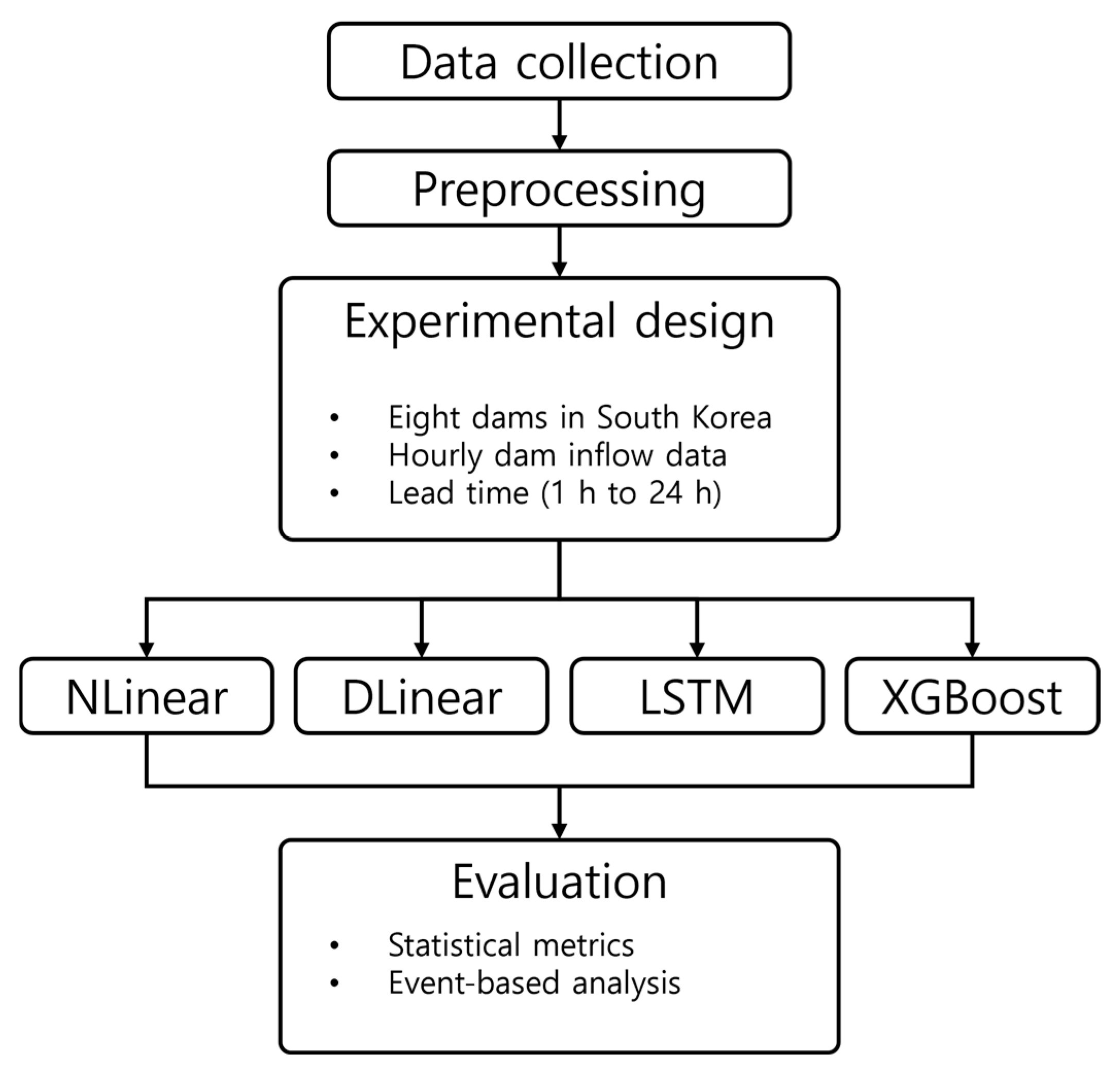
The experimental framework (Figure 3) comprises four main stages: data collection and preprocessing, model training, performance evaluation, and spatial analysis. WAMIS and UNESCO IHP data were preprocessed to handle missing values, normalize features, and generate input sequences. Four forecasting models—NLinear, DLinear, LSTM, and XGBoost—were trained and evaluated using both statistical metrics (nRMSE, nMAE, R², mBias, and KGE) and event-based analyses. Spatial grouping and reliable lead time classification were then applied to provide operational reservoir management insights.

Figure 3. Schematic workflow of the experimental framework.

2.3.1. Input Window Size and Data Partitioning

The input window length was set to 24 h for all models. A sensitivity analysis was conducted to examine the effect of window length on forecasting performance before determining this value. Window sizes ranging from 24 to 720 h were evaluated using the DLinear model as a representative baseline. Although the optimal window size varied slightly among basins, the 24 h window generally provided the most stable and favorable performance in most basins.

This study aims to systematically compare multiple prediction models under consistent and fair experimental conditions, despite the input window for each basin and model. Thus, adopting a uniform window length prevents the effects of model- and basin-specific tuning and ensures methodological comparability.

All datasets were divided sequentially into training (70%), validation (15%), and testing (15%) subsets to preserve temporal structure. The validation and test periods were selected from non-overlapping, chronologically subsequent intervals to avoid information leakage. Differences in total sample size occurred in some basins due to missing observations.

2.3.2. LTSF-Linear Models

The NLinear and DLinear models were implemented following the standard LTSF-Linear framework. For DLinear, the moving-average window was set to 6 h to extract short-term trends. Both models were trained using the Adam optimizer (learning rate = 0.001) with the mean squared error (MSE) as the loss function. Training continued until the validation loss stabilized rather than applying explicit early stopping. The final parameters were selected based on the minimum validation loss.

2.3.3. LSTM Model

For comparison, an LSTM model was constructed under the same experimental configuration (24 h input, 24 h forecast) and data split scheme. The network consisted of a single hidden layer with 10 units and no dropout. The Adam optimizer (learning rate = 0.001) and MSE loss were employed. Before training, the input data were normalized to the range [0, 1], and all evaluation metrics were computed after inverse normalization to restore physical units. The model was trained until the validation loss stabilized, and the best-performing model was selected based on the minimum validation loss.

2.3.4. XGBoost

The XGBoost model [39] was used as the baseline machine learning approach for comparison with the deep learning models. Under the same input–output configuration (24 h input and 24 h forecast) and data split scheme described in Section 3.1, the input time series was converted into supervised learning samples using a sliding-window method.

A direct multi-step forecasting strategy was adopted, in which a separate XGBoost regression model was trained independently for each forecast horizon (1 to 24 h ahead). Each model was trained using 1000 boosting trees, a learning rate of 0.03, a maximum tree depth of 5, and subsampling rates of 0.8 for both samples and features. The hist algorithm was used for efficient tree construction. Validation performance was monitored during training. Although all basins shared identical observation periods, the presence of missing values in some inflow records led to minor differences in the total number of available samples across basins.

2.4. Performance Metrics

Multiple statistical and hydrological indicators were employed to evaluate the performance of the model. These metrics assess different predictive accuracy, bias, and hydrological consistency aspects. While RMSE, MAE, and R² are widely used, KGE has gained prominence because it integrates correlation (ρ), variability ratio (α), and bias ratio (β) into a single index [40,41]. Conventional benchmarks such as R² ≈ 0.5 or NSE > 0.5 are often treated as “satisfactory” guidelines [42,43]; however, metric choice can alter model rankings, underscoring the need for a multi-metric evaluation framework [40,44].

2.4.1. Normalized Root Mean Square Error (nRMSE)

The nRMSE was defined as the RMSE normalized by the mean of the observed values, representing the relative magnitude of prediction errors. Because its unit was standardized, it allowed performance comparison across different catchments or periods [45]. Since nRMSE was derived from RMSE, it exhibited similar characteristics. RMSE was calculated by squaring the errors, averaging them, and then taking the square root; thus, it was more sensitive to large errors (outliers) [45]. When the differences between certain observed and predicted values were large, the RMSE tended to be greater than the average error magnitude. This made RMSE particularly useful in model performance evaluation when extreme errors were the emphasis.

$$nRMSE={\displaystyle \frac{\sqrt{\frac{1}{N}{\sum }_{i=1}^N{(y_i-\widehat{y_i})}^2}}{\overline{y_i}}}$$

(13)

2.4.2. Normalized Mean Absolute Error (nMAE)

The MAE was defined as the mean of the absolute errors between observed and predicted values, providing an intuitive measure of error magnitude. Because the MAE assigned equal weights to all errors, it was less affected by extreme values and represented the typical error magnitude in a more stable manner [46]. In cases where the error distribution was skewed or outliers existed, the MAE provided a representative value closer in nature to the median than the mean [45]. Therefore, the MAE was suitable for intuitively assessing the average predictive accuracy.

$$MAE={\displaystyle \frac{1}{N}}{\sum }_{i=1}^N\left|y_i-\widehat{y_i}\right|, nMAE={\displaystyle \frac{\frac{1}{N}{\sum }_{i=1}^N\left|y_i-\widehat{y_i}\right|}{\overline{y_i}}}$$

(14)

2.4.3. Coefficient of Determination (R²)

The coefficient of determination ($R^2$) represents the proportion of the variance in the observed values explained by the predictions. An $R^2$ value close to 1 indicated that the predictive model explained the variability of the observations well [47].

$$R^2=1-{\displaystyle \frac{\frac{1}{N}{\sum }_{i=1}^N{(y_i-\widehat{y_i})}^2}{\frac{1}{N}{\sum }_{i=1}^N{(y_i-\overline{y_i})}^2}}$$

(15)

2.4.4. Mean Bias (mBias)

The mBias expressed the mean difference between predicted and observed values as a ratio, thereby identifying the tendency of predictions to be over-or underestimated. A positive mBias indicated an overestimation, while a negative mBias indicated an underestimation [42].

$$mBias(\mathrm{\%})={\displaystyle \frac{{\sum }_{i=1}^N(y_i-\widehat{y_i})}{{\sum }_{i=1}^N{y}_i}}\times 100$$

(16)

2.4.5. Kling–Gupta Efficiency (KGE)

The KGE, introduced by Gupta et al. [40], evaluated model skill by integrating correlation, variability, and bias into a single index; values nearer 1 signified better agreement. It was widely applied in hydrology and water resources forecasting [40].

$$KGE=1-\sqrt{{(r-1)}^2+{(\beta -1)}^2+{(\gamma -1)}^2}$$

(17)

where $r$ is the correlation coefficient between observed and simulated values. $\beta ={\displaystyle \frac{{\mu }_s}{{\mu }_0}}$ is the bias ratio, where ${\mu }_s$ is the mean of simulated values and ${\mu }_0$ is the mean of observed values. $\gamma ={\displaystyle \frac{C{V}_s}{C{V}_0}}={\displaystyle \frac{{{\sigma }_s/\mu }_s}{{\sigma }_0/{\mu }_0}}$ is the variability ratio, where $C{V}_s$ and $C{V}_0$ are the coefficients of variation in simulated and observed values, respectively.

3. Results

Hourly inflow data from eight dams were used to evaluate four forecasting models—NLinear, DLinear, LSTM, and XGBoost—under a 24 h prediction horizon. Model performance was assessed using nRMSE, nMAE, R², mBias, and KGE. In particular, R and mBias were used to interpret the correlation and bias components contributing to KGE, while nRMSE and nMAE reflected variability representation. The overall performance evaluation results of the models are summarized in Table 2.

Table 2. Average evaluation metrics across all sites and the full evaluation period (lead times 1–24 h). Underline indicates the best performance among four models based on each evaluation metric.

Metric	Nlinear	Dlinear	LSTM	XGBoost
RMSE	79.2	74.9	73.5	82.1
nRMSE	2.0	1.9	1.8	2.3
MAE	35.3	34.3	35.8	36.4
nMAE	0.75	0.75	0.79	0.86
mBias	−0.07	0.8	−5.53	−6.01
R2	0.3	0.4	0.43	0.04
R	0.60	0.62	0.66	0.66
KGE	0.57	0.39	0.51	0.42

Across all sites and lead times, LSTM achieved the best performance in terms of RMSE, nRMSE, and R², whereas DLinear produced the lowest nMAE. NLinear outperformed the other models in mBias and KGE, reflecting its strength in balancing correlation, bias, and variability. The higher KGE of NLinear can be explained by its balanced performance across these components, as indicated by its moderate error levels (nRMSE), low mean bias, and stable temporal coherence (R²). XGBoost showed comparatively lower performance across most metrics, serving as a baseline reference for evaluating the improvements achieved by the sequence-based forecasting models. These results highlight that model strengths are metric-dependent: LSTM performed best in correlation and overall error reduction (R², nRMSE), DLinear minimized absolute errors (MAE, nMAE), and NLinear achieved superior balance through higher KGE and lower mBias.

3.1. Lead Time Dependence and Reliability

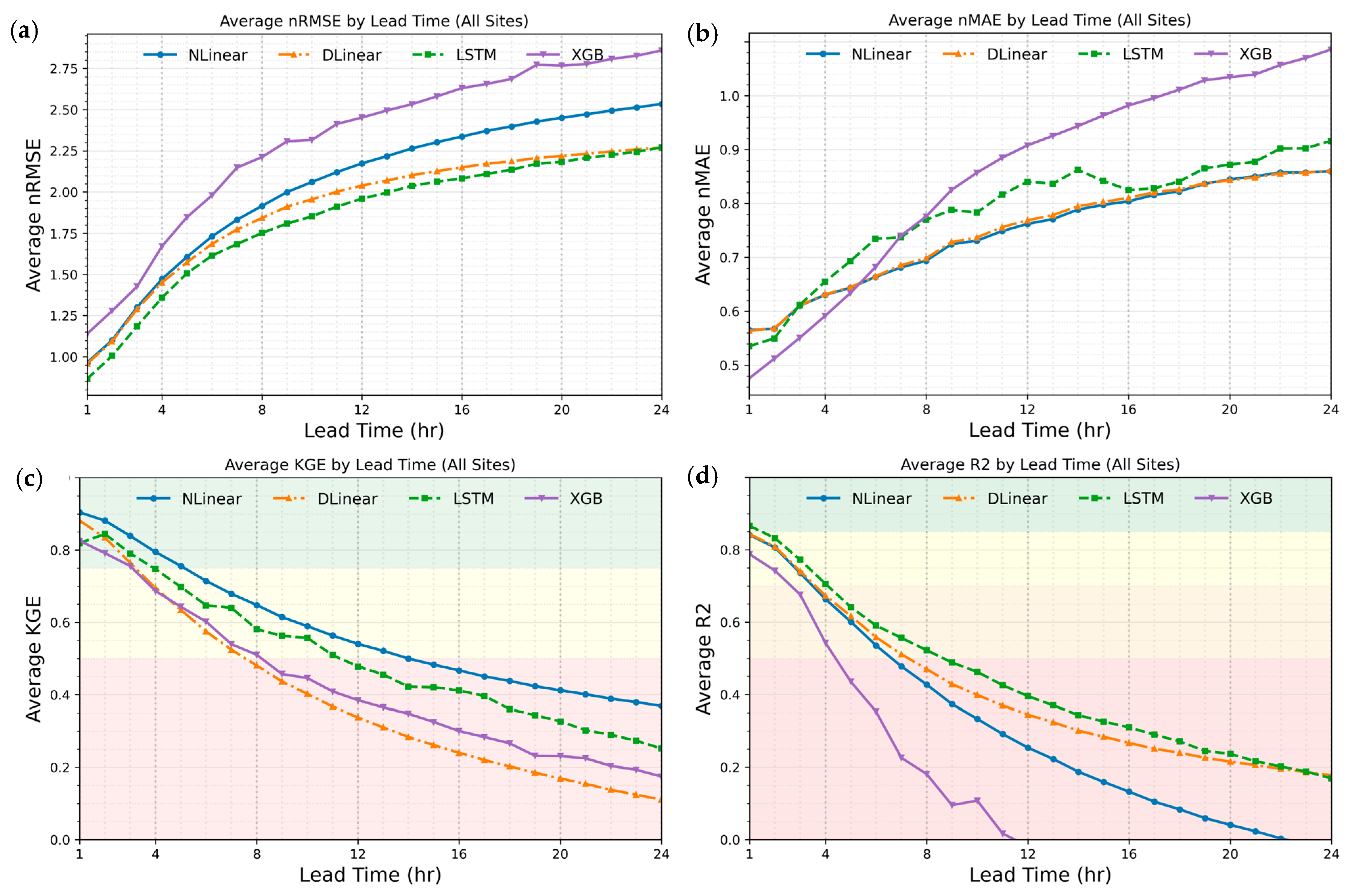
Figure 4 presents the average prediction performance for different models and lead times. The predictive performance varied with the lead time. LSTM maintained the lowest nRMSE across most horizons, although its performance converged with DLinear after approximately 22 h. DLinear yielded the lowest nMAE beyond 2 h, while LSTM performed best for very short horizons (1–2 h). In terms of KGE, NLinear consistently achieved the highest values, whereas LSTM degraded more rapidly as the lead time increased. R² results confirmed the overall superiority of LSTM, particularly beyond 18 h. XGBoost showed the lowest performance across all lead times, with larger increases in nRMSE and nMAE and a more rapid decline in R² and KGE as the forecast horizon increased.

Figure 4. Average prediction performance for different models and lead times (1–24 h) for (a) nRMSE, (b) nMAE, (c) KGE, and (d) R².

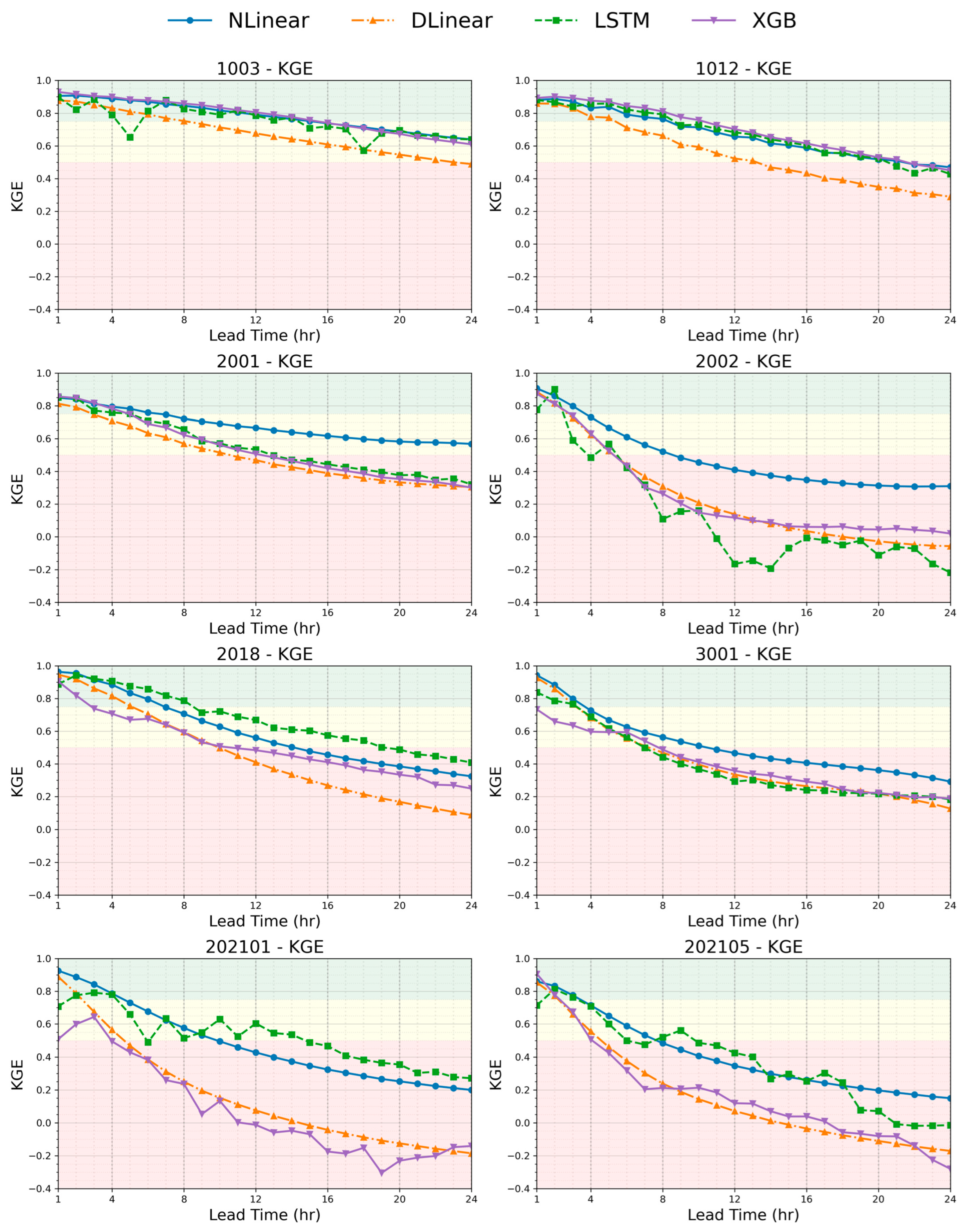
Figure 5 and Figure 6 illustrated the $R^2$ and KGE values across lead times for each study site. In this study, threshold values were established for performance evaluation: $R^2$ ≥ 0.5 followed the recommended guideline for hydrological model evaluation [43], while KGE ≥ 0.5 was adopted as the widely used boundary for “satisfactory/acceptable” performance in previous studies [48,49]. Although XGBoost was included as a baseline reference model, its R² values declined sharply with increasing lead time—particularly at sites 2002, 202101, and 202105—falling well below the acceptable threshold. Therefore, the threshold-based reliability analysis focused on the four sequence-based models (NLinear, DLinear, LSTM, and XGBoost), for which performance remained within the interpretable range across lead times.

Figure 5. Lead time curves of R² (1–24 h) for each study site.

Figure 6. Lead time curves of KGE (1–24 h) for each study site.

For the 24 model–site combinations (8 sites × 3 models), the proportion of cases exceeding the thresholds varied with lead time. Based on the $R^2$ criterion, 54.2% met the threshold at 6 h, but the proportion sharply declined to 12.5% at 12 h, 8.3% at 18 h, and 0% at 24 h. In contrast, according to the KGE criterion, 75% satisfied the threshold at 6 h, 46% at 12 h, 29.2% at 18 h, and 12% at 24 h, indicating that although performance decreased markedly beyond 12 h, several combinations still maintained acceptable levels at 24 h.

When comparing the median maximum reliable lead time by model, the $R^2$-based criterion showed LSTM (9.0 h) > DLinear (6.5 h) > NLinear (6.0 h), indicating that the LSTM maintained reliable predictive skill over a longer horizon. Under the KGE criterion, however, NLinear (11.0 h) ≈ LSTM (11.0 h) > DLinear (8.5 h), suggesting that NLinear and LSTM were more advantageous when correlation, bias, and variability were comprehensively considered.

At the site level, the longest maximum reliable lead time by the $R^2$ criterion was observed at site 1003 (20 h), with model-specific values of 17/20/22 h (NLinear/DLinear/LSTM). In contrast, the shortest lead times were recorded at sites 2002, 202105, and 3001, all with 4 h; the model-specific values were 4/4/5 h, 4/4/4 h, and 4/4/6 h, respectively. Under the KGE criterion, site 1003 again exhibited the longest maximum reliable lead time (24 h), with values of 24/23/24 h (NLinear/DLinear/LSTM), while site 2002 had the shortest value (5 h), with model-specific values of 8/5/5 h (NLinear/DLinear/LSTM).

Overall, the maximum reliable lead time was concentrated around 6 h when using the $R^2$ criterion and around 10–12 h when using the KGE criterion. Beyond 18 h, the variability across sites and models increased substantially.

3.2. Per-Site Boxplots of Model Performance Across Lead Times (1–24 h), Site Grouping, and Peak Reproduction

Figure 7 presents site-wise boxplots of model performance across lead times (1–24 h). For nRMSE, the LSTM generally exhibited lower median values and a narrower interquartile range (IQR), indicating more stable performance. DLinear showed comparatively lower nMAE values at several sites. In contrast, XGBoost displayed wider IQRs and lower median values across many sites, reflecting greater variability and reduced overall accuracy.

Figure 7. Site-specific distributions of nRMSE, nMAE, KGE, and R² across lead times (1–24 h). Boxes indicate the IQR with the median; whiskers show variability across lead times.

For R² and KGE, clear site-to-site differences were observed. At sites where the IQR crossed the threshold value of 0.5, performance reliability varied depending on the lead time. Conversely, sites with IQRs entirely above or below the threshold showed consistently high or low performance, respectively. These distributional characteristics provide information on performance level (median), stability (IQR), and range of variation (whiskers), which cannot be captured by single mean-based metrics, and thus support the determination of site-specific reliable lead times. Based on the distribution patterns of R² and KGE relative to the threshold value of 0.5, the study sites were grouped into three categories.

The high-performing category included Site 1003, where both the median and IQR of R² and KGE remained consistently above 0.5, indicating stable forecasting performance across all lead times. The transitional category comprised Sites 1012 and 2001, where the medians approached the threshold and the IQRs crossed 0.5, reflecting lead-time-dependent performance variability. The vulnerable category consisted of Sites 2018, 202101, 2002, 3001, and 202105, where both the median and IQR were predominantly below 0.5, indicating limited predictive capability across most lead times.

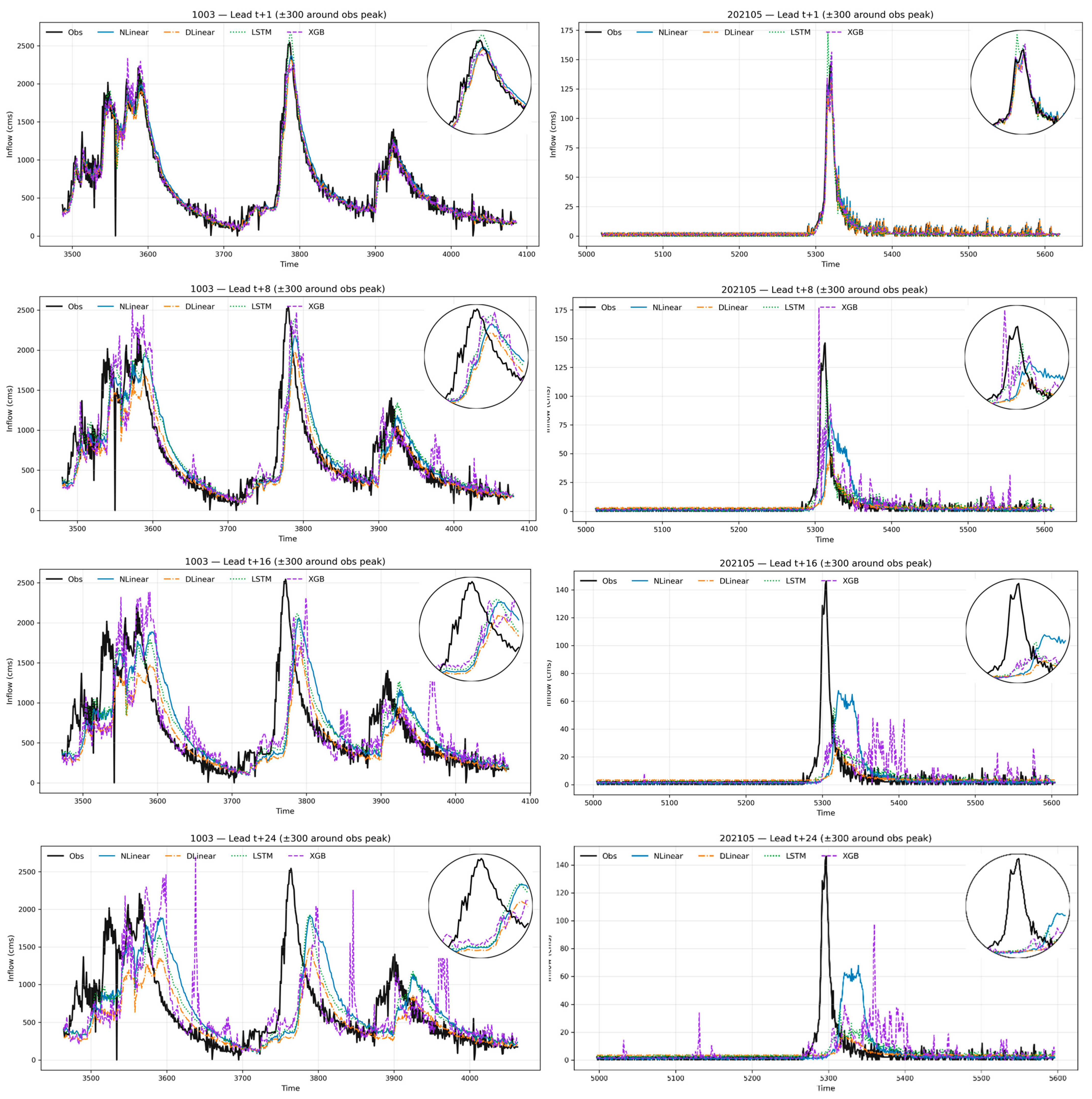
Figure 8 compares peak inflow reproducibility at sites 1003 and 202105 across lead times (1, 8, 16, and 24 h). At t + 1, the models show distinct peak behaviors: LSTM tends to produce slightly higher peak magnitudes than observation, while NLinear and DLinear yield smoother and lower peak estimates. XGBoost exhibits local amplitude fluctuations around the peak. As lead time increases, all models show reduced peak sharpness and increasing temporal lag, with the degree of peak smoothing most pronounced in DLinear and the variability most evident in XGBoost. These differences are more severe at site 202105 than at 1003, consistent with the site-level performance patterns identified earlier.

Figure 8. Peak inflow reproduction at short and long forecast horizons (t + 1, t + 8, t + 16, t + 24) for Miryang (202105) and Chungju (1003) sites. Black lines represent observations; blue, orange, and green lines show forecasts from NLinear, DLinear, and LSTM, XGBoost models, respectively. Insets provide detailed views of peak timing and magnitude accuracy.

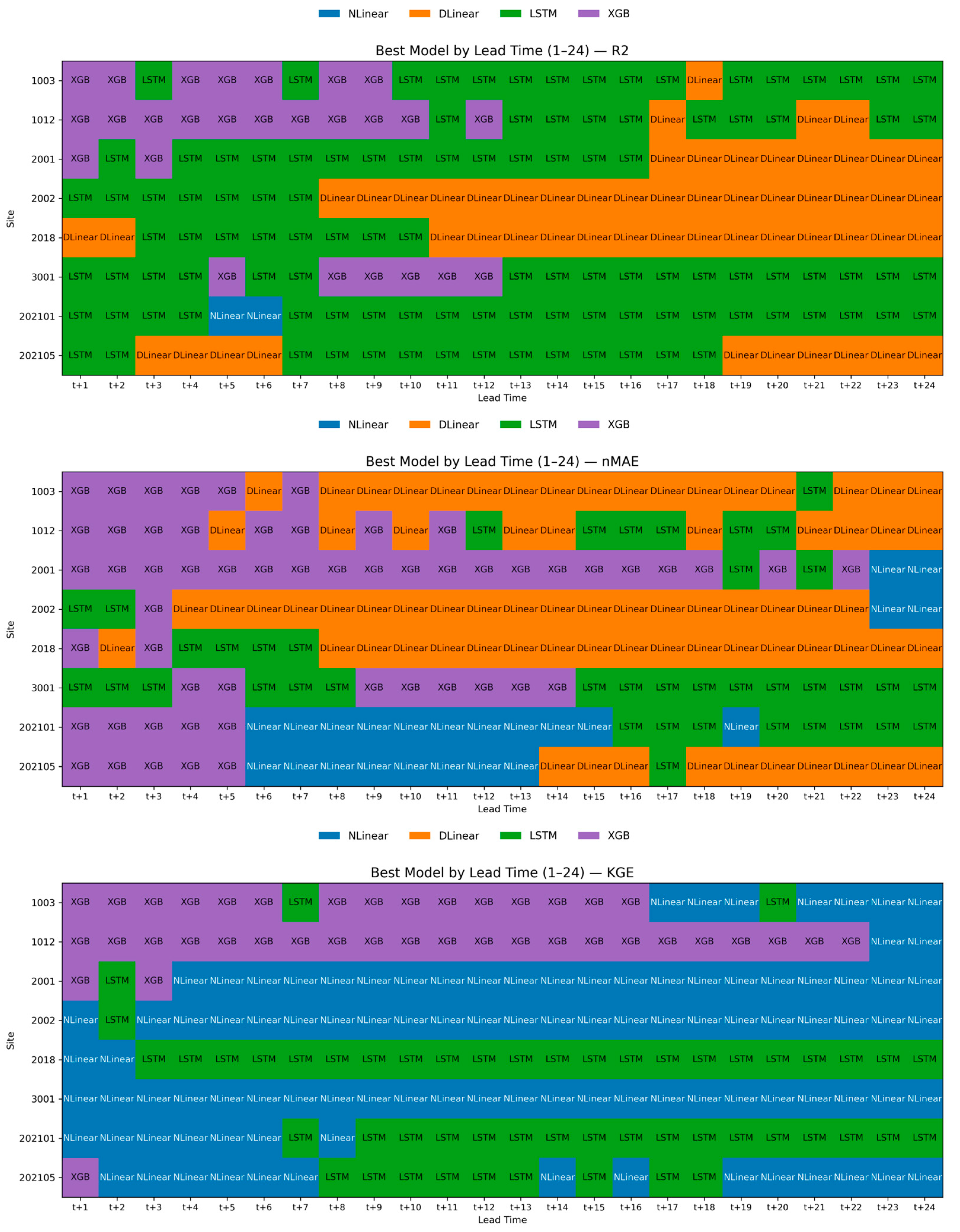
Figure 9 summarizes the proportion of lead times where each model performed best according to different indicators. For R², LSTM showed the highest proportion at 56.8%, with DLinear (28.6%) and XGB (13.5%) following. Under nMAE, DLinear was most frequent at 38.5%, followed by XGB (28.6%), LSTM (20.8%), and NLinear (12.0%). Under the KGE metric, NLinear accounted for 52.1 of the lead times, followed by LSTM (27.1%) and XGB (20.8%). These results indicate that model superiority varied depending on the evaluation metric: LSTM was more effective in reproducing correlation, DLinear tended to reduce absolute errors, and NLinear excelled in balancing correlation, bias, and variability. This demonstrates that no single model consistently outperformed the others across all criteria, and that the choice of evaluation metric directly influenced which model appeared most suitable.

Figure 9. Best-performing model by metric and lead time (t + 1–t + 24) across all sites. Panels: (top) R², (middle) nMAE, (bottom) KGE. Color key: NLinear (blue), DLinear (orange), LSTM (green), XGB (purple).

4. Discussion

4.1. Main Findings and Implications

Our evaluation showed that no single model consistently dominated across metrics. LSTM achieved the best R² and nRMSE, DLinear minimized MAE and nMAE, and NLinear performed best in KGE while maintaining balanced bias. These differences underline the metric-dependence of model ranking and stress the importance of multi-metric evaluation with explicit selection principles for robust hydrological forecasting.

To further quantify computational efficiency, we benchmarked the three models on an NVIDIA GeForce RTX 4070 Ti SUPER GPU using an identical batch size and data configuration. The average training time per epoch was 0.0013 s for NLinear, 0.0014 s for DLinessar, and 0.0023 s for LSTM, consistent with their analytical MACs (576, 1152, and 10,800, respectively). Inference latency per sample was 0.00038 ms (NLinear), 0.00062 ms (DLinear), and 0.00090 ms (LSTM). Accordingly, the linear models achieved approximately 1.6–1.8× faster training and 1.5–2.4× faster inference compared to LSTM. Regarding forecast horizons, performance was generally reliable within 6–12 h based on the widely used R²/KGE threshold of 0.5 [43]. Beyond 18–24 h, predictive skill degraded sharply due to weakened correlation and growing bias and variance. This suggests that forecasts shorter than 12 h can be directly applicable, while longer horizons may require post-processing or additional predictors such as rainfall forecasts.

Per-site revealed pronounced spatial heterogeneity despite the use of identical dam inflow inputs. Beyond mean values, the IQRs and whiskers highlighted horizon-dependent shifts in reliability and enabled classification into High-performing (1003), Transitional (1012, 2001), and Vulnerable (2018, 202101, 2002, 3001, 202105) site groups. The High-performing site maintained reliable predictive skill over extended lead times (≥12 h), whereas the Transitional sites exhibited moderate reliability within approximately 6–12 h depending on lead time. In contrast, the Vulnerable sites showed limited predictive performance, with reliability generally restricted to ≤6 h. These findings indicate limited transferability of model performance across locations and underscore the need for site-specific calibration and explicit communication of uncertainty through distribution-based metrics (IQR and whiskers), rather than relying solely on mean-based indicators.

This spatial variability in model performance can be attributed to distinct regional hydrometeorological characteristics across South Korea. High-performing sites, such as Chungju (1003) and transitional sites, such as Soyang (1012), are located in northern mountainous basins, where short-term flow fluctuations are moderated by delayed hydrographs and large storage capacities. In contrast, vulnerable southern basins, including Namgang (2018) and Miryang (202105), are strongly influenced by short-duration, high-intensity monsoon rainfall, leading to steep runoff responses and rapid changes in inflow. These regional contrasts align with recent climatological studies reporting intensified extreme rainfall and increased hydroclimatic instability in southern Korea during the summer monsoon [50,51]. This correspondence between model skill patterns and climatic conditions suggests that the observed spatial heterogeneity reflects genuine hydrometeorological differences, rather than data-driven artifacts, reinforcing the need for region-specific calibration in operational forecasting.

Beyond spatial patterns, performance rankings also varied depending on the evaluation metric used. The apparent superiority of each model shifted with the chosen criterion: LSTM achieved the highest proportion of top results under R² (56.8%), DLinear under nMAE (38.5%), and NLinear under KGE (52.1%). These metric-dependent rankings indicate that each model captures different aspects of hydrological behavior. This observation aligns with that of Cinkus et al. [52], who emphasized that interpretation should account for which dimensions of model behavior a given metric prioritizes.

Additionally, the reproducibility of peak inflow events declined as the lead time forecast increased. This pattern was consistently observed across sites in our experiments and has also been reported in previous hydrological deep learning studies, where data-driven models tended to capture the overall hydrograph while showing weaker skill in peak magnitude and timing at longer horizons [27,53] This suggests that the reduced peak fidelity observed here reflects a broader characteristic of sequence-based hydrological forecasting models rather than a limitation specific to the present approach.

In summary, model performance varies with the interaction of architecture, metric, and site. The findings highlight three key implications: (i) metric choice critically shapes conclusions, (ii) linear models offer substantial efficiency advantages, and (iii) spatial heterogeneity constrains direct model transfer. Addressing these aspects will be essential for advancing robust and operational hydrological forecasting.

4.2. Limitations

This study has three key limitations. First, it relied solely on a single predictor (dam inflow), without incorporating additional hydrometeorological or operational variables. Second, the analysis was limited to eight dam basins in South Korea, representing relatively narrow ranges of basin size, climate, and hydrological characteristics. Third, a fixed input window (24 h) and forecast horizon (24 h) were used for all experiments, without tuning to basin-specific response patterns.

As a result, the findings should be interpreted primarily as a controlled comparison across models under common conditions, rather than as a fully generalized assessment across diverse hydrological settings. Ensuring wider applicability will require the inclusion of multivariate predictors, larger and more diverse basin samples, and adaptive model configurations.

5. Conclusions

This study compared two LTSF-Linear models (NLinear, DLinear) with an LSTM and XGBoost for hourly dam inflow forecasting in South Korea, evaluated over 24 h horizons using multiple performance metrics. The results showed that model superiority was metric-dependent: LSTM achieved the best R² and nRMSE, DLinear minimized nMAE, and NLinear performed best in KGE.

Threshold-based evaluation (R², KGE ≥ 0.5) indicated that forecasts were generally reliable within short lead times (approximately 1–6 h), while performance gradually decreased in the 6–12 h range and degraded more noticeably beyond 12–24 h. Site-specific boxplots highlighted substantial spatial heterogeneity, leading to the classification of dams into high-performing, transitional, and vulnerable groups. These patterns demonstrate the limited transferability of models and the need for site-specific calibration.

Overall, the study concludes that (i) the LTSF-Linear models have a potential to be an alternative method for hydrological variable modeling, (ii) model–metric matching is critical for fair evaluation, (iii) operationally reliable forecasts are typically restricted to the short-term range (≤6 h), and (iv) longer horizons (>12 h) require post-processing, hybrid, or horizon-dependent correction strategies.

Future research should investigate the performance of LTSF models in representing a broader range of hydrological variables and phenomena. Incorporating multivariate predictors (e.g., rainfall, reservoir operations, and water levels), developing peak-aware loss functions, and adopting transfer learning approaches would contribute to advancing our understanding of AI-based modeling of hydrological processes.

References

- IPCC. Climate Change 2021: The Physical Science Basis; Cambridge University Press: Cambridge, UK, 2021. [Google Scholar] [CrossRef]
- Zarei, M.; Bozorg-Haddad, O.; Baghban, S.; Delpasand, M.; Goharian, E.; Loáiciga, H.A. Machine-Learning Algorithms for Forecast-Informed Reservoir Operation (FIRO) to Reduce Flood Damages. Sci. Rep. 2022, 12, 346. [Google Scholar] [CrossRef] [PubMed]
- Delaney, C.J.; Hartman, R.K.; Mendoza, J.; Dettinger, M.; Delle Monache, L.; Jasperse, J.; Ralph, F.M.; Talbot, C.; Brown, J.; Reynolds, D.; et al. Forecast-Informed Reservoir Operations Using Ensemble Streamflow Predictions for a Multipurpose Reservoir in Northern California. Water Resour. Res. 2020, 56, e2019WR026604. [Google Scholar] [CrossRef]
- Anghileri, D.; Voisin, N.; Castelletti, A.; Nijssen, B.; Lettenmaier, D.P. Value of Long-Term Streamflow Forecasts to Reservoir Operations. Water Resour. Res. 2016, 52, 4209–4225. [Google Scholar] [CrossRef]
- Wang, Q.J.; Bennett, J.C.; Robertson, D.E.; Shrestha, D.L.; Hapuarachchi, H.A.P. Improving Real-Time Reservoir Operation During Floods Using Inflow Forecasts. J. Hydrol. 2021, 598, 126017. [Google Scholar] [CrossRef]
- Ficchì, A.; Perrin, C.; Andréassian, V. Impact of Temporal Resolution of Inputs on Hydrological Model Performance: An Analysis Based on 2400 Flood Events. J. Hydrol. 2016, 538, 454–470. [Google Scholar] [CrossRef]
- Box, G.E.P.; Jenkins, G.M.; Reinsel, G.C.; Ljung, G.M. Time Series Analysis: Forecasting and Control; John Wiley & Sons: Hoboken, NJ, USA, 2015. [Google Scholar]
- Salas, J.D. Analysis and Modeling of Hydrologic Time Series. In Handbook of Hydrology; Maidment, D.R., Ed.; McGraw-Hill: New York, NY, USA, 1993; pp. 19.1–19.72. [Google Scholar]
- Hipel, K.W.; McLeod, A.I. Time Series Modelling of Water Resources and Environmental Systems; Elsevier: Amsterdam, The Netherlands, 1994. [Google Scholar]
- Zhang, G.P. Time Series Forecasting Using a Hybrid ARIMA and Neural Network Model. Neurocomputing 2003, 50, 159–175. [Google Scholar] [CrossRef]
- Montanari, A.; Brath, A. A Stochastic Approach for Assessing the Uncertainty of Rainfall–Runoff Simulations. Water Resour. Res. 2004, 40, W01106. [Google Scholar] [CrossRef]
- Abrahart, R.J.; See, L. Comparing Neural Network and Autoregressive Moving Average Techniques for the Provision of Continuous River Flow Forecasts in Two Contrasting Catchments. Hydrol. Process. 2000, 14, 2157–2172. [Google Scholar] [CrossRef]
- Yoon, H.; Jun, S.C.; Hyun, Y.; Bae, G.O.; Lee, K.K. A Comparative Study of Artificial Neural Networks and Support Vector Machines for Predicting Groundwater Levels in a Coastal Aquifer. J. Hydrol. 2011, 396, 128–138. [Google Scholar] [CrossRef]
- Granata, F.; Gargano, R.; De Marinis, G. Support Vector Regression for Rainfall–Runoff Modeling in Urban Drainage: A Comparison with the EPA’s Storm Water Management Model. Water 2016, 8, 69. [Google Scholar] [CrossRef]
- Cutler, D.R.; Edwards, T.C.; Beard, K.H.; Cutler, A.; Hess, K.T.; Gibson, J.; Lawler, J.J. Random Forests for Classification in Ecology. Ecology 2007, 88, 2783–2792. [Google Scholar] [CrossRef]
- Friedman, J.H. Greedy Function Approximation: A Gradient Boosting Machine. Ann. Stat. 2001, 29, 1189–1232. [Google Scholar] [CrossRef]
- Kim, T.; Shin, J.-Y.; Kim, H.; Kim, S.; Heo, J.-H. The use of Large-Scale Climate Indices in Monthly Reservoir Inflow Forecasting and Its Application on Time Series and Artificial Intelligence Models. Water 2019, 11, 374. [Google Scholar] [CrossRef]
- Natekin, A.; Knoll, A. Gradient Boosting Machines, a Tutorial. Front. Neurorobot. 2013, 7, 21. [Google Scholar] [CrossRef] [PubMed]
- Maier, H.R.; Jain, A.; Dandy, G.C.; Sudheer, K.P. Methods Used for the Development of Neural Networks for the Prediction of Water Resource Variables in River Systems: Current Status and Future Directions. Environ. Model. Softw. 2010, 25, 891–909. [Google Scholar] [CrossRef]
- Mosavi, A.; Ozturk, P.; Chau, K.W. Flood Prediction Using Machine Learning Models: Literature Review. Water 2018, 10, 1536. [Google Scholar] [CrossRef]
- Kim, T.; Shin, J.-Y.; Kim, H.; Heo, J.-H. Ensemble-based neural network modeling for hydrologic forecasts uncertainty in the model structure and input variable selection. Water Res. Res. 2020, 56, e2019WR026262. [Google Scholar] [CrossRef]
- Hochreiter, S.; Schmidhuber, J. Long Short-Term Memory. Neural Comput. 1997, 9, 1735–1780. [Google Scholar] [CrossRef]
- Kratzert, F.; Klotz, D.; Brenner, C.; Schulz, K.; Herrnegger, M. Rainfall–Runoff Modelling Using Long Short-Term Memory (LSTM) Networks. Hydrol. Earth Syst. Sci. 2018, 22, 6005–6022. [Google Scholar] [CrossRef]
- Mok, J.Y.; Choi, J.H.; Moon, Y.I. Prediction of Multipurpose Dam Inflow Using Deep Learning. J. Korea Water Resour. Assoc. 2020, 53, 881–892. [Google Scholar] [CrossRef]
- Le, X.H.; Ho, H.V.; Lee, G.; Jung, S. Application of Long Short-Term Memory (LSTM) Neural Network for Flood Forecasting. Water 2019, 11, 1387. [Google Scholar] [CrossRef]
- Lee, T.; Shin, J.-Y.; Kim, J.-S.; Singh, V.P. Stochastic Simulation on Reproducing Long-term Memory of Hydroclimatological Variables using Deep Learning Model. J. Hydrol. 2020, 582, 124540. [Google Scholar] [CrossRef]
- Xiang, Z.; Yan, J.; Demir, I. A Rainfall–Runoff Model with LSTM-Based Sequence-to-Sequence Learning. Water Resour. Res. 2020, 56, e2019WR025326. [Google Scholar] [CrossRef]
- Kratzert, F.; Herrnegger, M.; Klotz, D.; Hochreiter, S.; Klambauer, G. NeuralHydrology—Interpreting LSTMs in Hydrology. In Explainable AI: Interpreting, Explaining and Visualizing Deep Learning; Samek, W., Montavon, G., Vedaldi, A., Hansen, L., Muller, K.R., Eds.; Lecture Notes in Computer Science; Springer: Cham, Switzerland, 2019; Volume 11700. [Google Scholar] [CrossRef]
- Shen, C.; Laloy, E.; Elshorbagy, A.; Albert, A.; Bales, J.; Chang, F.J.; Ganguly, S.; Hsu, K.; Kifer, D.; Fang, K.; et al. HESS Opinions: Incubating Deep-Learning-Powered Hydrologic Science Advances as a Community. Hydrol. Earth Syst. Sci. 2018, 22, 5639–5656. [Google Scholar] [CrossRef]
- Reichstein, M.; Camps-Valls, G.; Stevens, B.; Jung, M.; Denzler, J.; Carvalhais, N.; Prabhat, F. Deep Learning and Process Understanding for Data-Driven Earth System Science. Nature 2019, 566, 195–204. [Google Scholar] [CrossRef]
- Giorgio, A.; Del Buono, N.; Berardi, M.; Vurro, M.; Vivaldi, G.A. Soil Moisture Sensor Information Enhanced by Statistical Methods in a Reclaimed Water Irrigation Framework. Sensors 2022, 22, 8062. [Google Scholar] [CrossRef]
- Gegenleithner, S.; Pirker, M.; Dorfmann, C.; Kern, R.; Schneider, J. Long Short-Term Memory Networks for Enhancing Real-Time Flood Forecasts: A Case Study for an Underperforming Hydrologic Model. Hydrol. Earth Syst. Sci. 2025, 29, 1939–1962. [Google Scholar] [CrossRef]
- Li, Z.; Qi, S.; Li, Y.; Xu, Z. Revisiting Long-Term Time Series Forecasting: An Investigation on Linear Mapping. arXiv 2023, arXiv:2305.10721. [Google Scholar] [CrossRef]
- Zeng, A.; Chen, M.; Zhang, L.; Xu, Q.; Sun, Q. Are Transformers Effective for Time Series Forecasting? In Proceedings of the AAAI Conference on Artificial Intelligence, Washington, DC, USA, 7–14 February 2023; Volume 37, pp. 11121–11128. [Google Scholar] [CrossRef]
- Lim, B.; Zohren, S. Time Series Forecasting with Deep Learning: A Survey. Philos. Trans. R. Soc. A 2021, 379, 20200209. [Google Scholar] [CrossRef] [PubMed]
- Ministry of Environment, Republic of Korea. Master Plan for National Water Management; Ministry of Environment: Sejong, Republic of Korea, 2021. Available online: https://water.go.kr/eng/515 (accessed on 15 September 2025).
- Water Resources Management Information System (WAMIS). Available online: http://www.wamis.go.kr (accessed on 15 September 2025).
- UNESCO IHP. South Korea Hydrometeorological Data from WAMIS. 2025. Available online: https://ihp-wins.unesco.org/en/dataset/south-korea-hydrometeorological-data-from-wamis (accessed on 16 September 2025).
- Chen, T.; Guestrin, C. XGBoost: A Scalable Tree Boosting System. In Proceedings of the 22nd ACM SIGKDD International Conference on Knowledge Discovery and Data Mining, San Francisco, CA, USA, 13 August 2016; pp. 785–794. [Google Scholar] [CrossRef]
- Gupta, H.V.; Kling, H.; Yilmaz, K.K.; Martinez, G.F. Decomposition of the Mean Squared Error and NSE/KGE Implications. J. Hydrol. 2009, 377, 80–91. [Google Scholar] [CrossRef]
- Vrugt, J.A.; de Oliveira, D.Y. Confidence Intervals of the Kling–Gupta Efficiency. J. Hydrol. 2022, 612, 127968. [Google Scholar] [CrossRef]
- Moriasi, D.N.; Arnold, J.G.; Van Liew, M.W.; Bingner, R.L.; Harmel, R.D.; Veith, T.L. Model Evaluation Guidelines for Systematic Quantification of Accuracy in Watershed Simulations. Trans. ASABE 2007, 50, 885–900. [Google Scholar] [CrossRef]
- Moriasi, D.N.; Gitau, M.W.; Pai, N.; Daggupati, P. Hydrologic and Water Quality Models: Performance Measures and Evaluation Criteria. Trans. ASABE 2015, 58, 1763–1785. [Google Scholar] [CrossRef]
- Knoben, W.J.M.; Freer, J.E.; Woods, R.A. Technical Note: Inherent Benchmark or Not? Comparing Nash–Sutcliffe and Kling–Gupta Efficiency Scores. Hydrol. Earth Syst. Sci. 2019, 23, 4323–4331. [Google Scholar] [CrossRef]
- Chai, T.; Draxler, R.R. Root Mean Square Error (RMSE) or Mean Absolute Error (MAE)?—Arguments against Avoiding RMSE in the Literature. Geosci. Model Dev. 2014, 7, 1247–1250. [Google Scholar] [CrossRef]
- Willmott, C.J.; Matsuura, K. Advantages of the Mean Absolute Error (MAE) over the Root Mean Square Error (RMSE) in Assessing Average Model Performance. Clim. Res. 2005, 30, 79–82. [Google Scholar] [CrossRef]
- Nash, J.E.; Sutcliffe, J.V. River Flow Forecasting through Conceptual Models Part I—A Discussion of Principles. J. Hydrol. 1970, 10, 282–290. [Google Scholar] [CrossRef]
- Laiti, L.; Mallucci, S.; Piccolroaz, S.; Bellin, A.; Zardi, D.; Fiori, A.; Nikulin, G.; Majone, B. Testing the Hydrological Coherence of High-Resolution Simulations: On KGE Use and Thresholds. Water Resour. Res. 2018, 54, 1618–1637. [Google Scholar] [CrossRef]
- Abdalla, E.M.H.; Alfredsen, K.; Muthanna, T.M. Towards Improving the Calibration Practice of Conceptual Hydrological Models of Extensive Green Roofs. J. Hydrol. 2022, 607, 127548. [Google Scholar] [CrossRef]
- Kim, H.R.; Moon, M.; Yun, J.; Ha, K.J. Trends and Spatio-Temporal Variability of Summer Mean and Extreme Precipitation across South Korea for 1973–2022. Asia-Pac. J. Atmos. Sci. 2023, 59, 385–398. [Google Scholar] [CrossRef]
- Seo, G.Y.; Min, S.K.; Lee, D.; Son, S.W.; Park, C.; Cha, D.H. Hourly Extreme Rainfall Projections over South Korea Using Convection Permitting Climate Simulations. npj Clim. Atmos. Sci. 2025, 8, 209. [Google Scholar] [CrossRef]
- Cinkus, G.; Mazzilli, N.; Jourde, H.; Wunsch, A.; Liesch, T.; Ravbar, N.; Chen, Z.; Goldscheider, N. When Best Is the Enemy of Good—Critical Evaluation of Performance Criteria in Hydrological Models. Hydrol. Earth Syst. Sci. 2023, 27, 2397–2411. [Google Scholar] [CrossRef]
- Kratzert, F.; Klotz, D.; Herrnegger, M.; Sampson, A.K.; Hochreiter, S.; Nearing, G.S. Toward Improved Predictions in Ungauged Basins: Exploiting the Power of Machine Learning. Water Resour. Res. 2019, 55, e2019WR026065. [Google Scholar] [CrossRef]
Disclaimer/Publisher’s Note: The statements, opinions and data contained in all publications are solely those of the individual author(s) and contributor(s) and not of MDPI and/or the editor(s). MDPI and/or the editor(s) disclaim responsibility for any injury to people or property resulting from any ideas, methods, instructions or products referred to in the content. |
© 2025 by the authors. Licensee MDPI, Basel, Switzerland. This article is an open access article distributed under the terms and conditions of the Creative Commons Attribution (CC BY) license (https://creativecommons.org/licenses/by/4.0/).