Article

Uncovering the Drivers of Urban Flood Reports: An Environmental and Socioeconomic Analysis Using 311 Data

by
Natalie R. Lerma
*,
Jonathan L. Goodall
* and
Julianne D. Quinn
Department of Civil and Environmental Engineering, University of Virginia, 151 Engineers Way, Box 400747, Charlottesville, VA 22904-4747, USA
*
Authors to whom correspondence should be addressed.
Water 2025, 17(21), 3178; https://doi.org/10.3390/w17213178
Submission received: 22 September 2025 / Revised: 27 October 2025 / Accepted: 30 October 2025 / Published: 6 November 2025
(This article belongs to the Special Issue Climate Risk Management, Sea Level Rise and Coastal Impacts)

Abstract

Cities use 311 platforms for residents to report flooding, offering insight into flood-prone areas. The combined role of environmental and socioeconomic factors shaping these reports remains unexplored. This study analyzes five years of 311 flood reports in Norfolk, VA, using a logistic regression model to identify salient predictors and assess their influence on flood reporting. The model includes environmental variables (precipitation, tide level, and topographic wetness index) and socioeconomic indicators (race, income, and education). The model performed well with an area under the receiver operator characteristic (ROC) curve (AUC) of 0.8. Permutation-based feature importance revealed precipitation as the most important predictor (AUC contribution: 0.27), followed by the percentage of Black residents (0.02); tide only contributed ~0.01. The influence of the percentage of Hispanics was also ~0.01. Increases in the percentage of Black residents were associated with increased reporting, while the converse was true for a higher percentage of Hispanic residents. Higher reporting in Norfolk from locations with more Black residents is distinct from findings in other cities, suggesting Norfolk may have more effective communication with these residents about 311 reporting. However, lower reporting in locations with more Hispanic residents suggests Norfolk could improve outreach to non-native speakers, for example, by adding Spanish language options to their 311 platform.

1. Introduction

The frequency and intensity of extreme weather events in the United States (US) have increased significantly since the 1980s, with the number of billion-dollar disasters rising over time [1]. Increases in extreme flood events have been observed due to the intensification of key hydrometeorological and oceanic drivers from climate change, including precipitation, storm surge, and sea level rise (SLR) [2,3].
In low-relief urban coastal environments, these flood drivers frequently interact, creating compounding flood hazards [3,4] that exacerbate flood impacts [5]. In particular, the combination of SLR and land subsidence (i.e., relative sea level rise (RSLR)) has led to increased frequency of nuisance flooding [6]. While not as immediately destructive as extreme events, recurrent nuisance flooding disrupts traffic networks [7,8], devalues property [9], and accelerates infrastructure degradation [10]. These chronic flood events result in cumulative economic and social costs that can rival or exceed those of less frequent, high-magnitude flood disasters [11].
Mapping the extent of flood events relies on earth observation (EO) data, such as land use, streamflow, and topographic datasets, and computational models to simulate flood dynamics. Traditional flood modeling approaches (e.g., one-dimensional (1D) hydrodynamic models) provide computationally efficient simulations of riverine systems but may be insufficient for representing complex flow interactions in low-gradient coastal landscapes [12,13,14,15,16,17]. Two-dimensional (2D) models offer improved spatial representation of overland flow [17,18], but their computational demands often limit real-time applications [19].
Despite efforts to enhance model efficiency and predictive capabilities [20,21,22], physical models remain constrained by data availability, as in situ environmental monitoring is geospatially sparse [23]. While the U.S. Geological Survey (USGS) and local agencies operate over 8000 stream gauges nationwide, nearly 400,000 streams and urban drainage systems lack real-time, consistent hydrologic observations [24]. Federal and local agencies lack the resources to fill this gap [25]. The National Water Model (NWM) extends hydrologic predictions to 2.7 million reaches [26], yet its resolution remains coarse for urban flood forecasting.
Remote sensing has improved the monitoring of Earth’s systems [27,28], with particular advancements in the field of hydrology. For instance, satellite-derived optical images are used to create data products that delineate flood extent; however, these optical images are impacted by spectral resolution and cloud cover, which can interfere with image collection and cast shadows during storm events [29,30,31,32]. To address this concern, researchers are investigating the use of synthetic aperture radar (SAR) to capture flood extent and flood depths [30,32,33,34,35]. However, SAR is inherently noisy and susceptible to surface conditions (e.g., wind-generated capillary waves, floating debris, and vegetation) [33]. While satellite-derived flood products are expanding global availability of EO, they rely on ground truthing via in situ sensors, which may not be available or not at the desired spatial resolution necessary for characterizing street flooding in urban environments.
Given the challenges of hydrologic data sparsity, crowd-sourced datasets have emerged as valuable supplements to traditional monitoring networks. User-reported transportation disruptions from Waze and social media platforms (e.g., X, BlueSky) have been integrated into flood modeling workflows to enhance situational awareness for dispatching relief resources and validating hydrodynamic simulations [36,37,38,39,40]. Personal weather stations (PWS) maintained by citizen scientists have also been used to improve the spatial resolution of precipitation data for stormwater modeling [41], though deployment costs and participation requirements pose challenges to the scalability [42].
Municipal 311 service requests are another underutilized crowdsourced resource for measuring urban flood extent and understanding infrastructure performance. Agonafir et al. studied the effects of precipitation and infrastructure on 311 floods but omitted other environmental variables (e.g., tide and TWI) and the role of socioeconomic factors [43]. Kontokosta et al. evaluated the role of socio-spatial patterns on propensity to complain, and while their study incorporated socioeconomic and infrastructure factors, they did not evaluate the influence of environmental datasets [44]. Other studies have focused on spatial patterns of service requests [45,46] and the use of meteorological conditions to predict stormwater-related complaints [46,47]. A comprehensive assessment of the combined influence of socioeconomic and environmental factors on flood-related 311 service requests has yet to be studied.
This study analyzes five years of 311 service requests for flooding stoppages (i.e., flood reports) in Norfolk, Virginia, to investigate the environmental and social drivers of urban flooding. It addresses the following research questions:
  • What are the most influential predictors in determining the likelihood of a flood report within the study area, as identified through permutation-based feature importance?
  • To what extent do racial demographic variables demonstrate influence on the prediction of flood reports, as assessed by permutation-based feature importance?
  • What is the direction of the relationship between specific racial demographic variables and the log-odds of a flood report, as indicated by the coefficients of the logistic regression model?
To answer these questions, this study evaluates the influence of socioeconomic, meteorological-oceanic, and topographic physical factors on flood-related service request occurrence. A logistic regression model is employed to determine the likelihood of a flood report, while permutation-based feature importance rankings are applied to rank predictor relevance. This study offers a novel application of 311 crowd-sourced data to identify flood-prone areas, analyze drivers of flood reporting, and examine environmental justice dimensions of urban flooding. Section 2 details the study area, data sources, and methods, followed by the results in Section 3. Section 4 discusses key findings, and Section 5 concludes with implications for urban flood monitoring and management.

2. Materials and Methods

2.1. Study Area

This study analyzes five years of 311 flood reports in Norfolk, Virginia, from October 2019 through December 2024. The City of Norfolk, VA, is a highly urbanized, low-relief coastal city and home to the world’s largest naval base. According to a report from the National Oceanic and Atmospheric Administration (NOAA), Norfolk has experienced a 325% increase in nuisance flood events since 1960, driven by climate-related SLR, land subsidence, and loss of natural barriers [48]. The study area is depicted in Figure 1, along with the tide gauge location used in this study. The spatial distribution of flood reports is also mapped in Figure 1.

2.2. Data and Preprocessing

Data from the newer 311 platform, MyNorfolk Portal, was downloaded in comma separated values (CSV) format from the City of Norfolk’s data management site [49]. Data preprocessing was conducted in Python Version 3.10 to extract the relevant service request category, “Stormwater.” Duplicate service requests were removed using unique address and timestamp information associated with the requests. Each request was geocoded using the University of Virginia’s (UVA’s) ArcGIS Online geocoding tool and assigned a census tract for integration with socioeconomic data.
Racial information for each service request location was obtained at the census tract level from the U.S. Census Bureau’s American Community Survey (ACS) 2017–2021 5-year estimates Table(s) B03002. To normalize population-dependent variables, racial demographic variables were converted to percentages of the total census tract population (White_alon_Pct, Black_or_A_Pct, Hispanic_o_Pct, Asian_Alone_Pct, Two_or_More_Pct, Some_Other_Pct). This transformation ensured comparability across tracts by preventing population size from influencing the model interpretation. Additionally, some racial groups were excluded from the study due to low representation across census tracts to reduce model dimensionality; Native American and American Indian residents were removed from the population count for each census tract. Education level for adults 25+ was obtained from the U.S. Census Bureau’s American Community Survey (ACS) 2015–2019 5-year estimates (Table(s) B15002). The original education classification included (1) Less than High School, (2) High School Graduate (includes equivalency), (3) Some College, No Degree, (4) Associate’s Degree, and (5) Bachelor’s Degree or Higher. Multicollinearity was observed among several adjacent categories, particularly between “Less than High School” and “High School Graduate,” as well as among the higher education groups (e.g., “Some College” and “Associate’s Degree”). To address this, classes were consolidated into two broader categories: (1) high school diploma (or equivalent) or less (HS_or_Less), and (2) some college or more (College_Plus). This grouping method is a recommended strategy for mitigating multicollinearity in regression modeling [50]. Median household income (Income) from the U.S. Census Bureau’s ACS 2019–2023 5-year estimates Table(s) B19013, B19049, and B19053 were used as a socioeconomic predictor in this study.
Precipitation data were collected from the National Center for Environmental Prediction’s (NCEP) EMC 4KM Gridded Data (GRIB) Stage IV rainfall dataset, accessed from the University Corporation for Atmospheric Research (UCAR)-National Center for Atmospheric Research (NCAR) Earth Observing Laboratory (EOL) [51]. Rainfall values (Precip) for each service request location were estimated using inverse distance weighting (IDW) interpolation, based on radar grid points within the bounding box: 76.36° W–76.12° W, 36.8° N—36.97° N. IDW assigns weights to observations inversely proportional to their distance raised to a power, here 1, prioritizing nearer points while maintaining spatial variation in precipitation at a resolution finer than the 4 km radar grid.
To simplify tidal assignments across 1701 unique service request coordinates, water level data from the Sewell’s Point station (Station ID: 8638610) were used uniformly across all locations. This will therefore capture temporal variability in the influence of tidal fluctuations on flood reports across flood events, but not spatial variability. While changes in sea level, such as those caused by astronomical tides, storm surges, and waves, can influence the spatial distribution of coastal urban flooding, the extent of tidally (i.e., water level)-driven flooding depends on built and natural features of the urban environment. As tides propagate through inlets, they are influenced by amplification (i.e., shoaling) due to shoreline and bathymetric features, energy losses (i.e., dissipation) from bottom friction with the bay, and partial reflection from the head of the bay [52]. If water levels rise sufficiently, they can block stormwater pipes from draining or push through the pipe network [6,53,54,55]. Analysis of these complex processes was beyond the scope of this paper, but could be explored in future work.
The topographic wetness index (TWI) was computed citywide at a 1 m resolution using a digital elevation model (DEM). TWI quantifies water accumulation potential based on terrain characteristics of elevation, slope, and upstream contribution. The workflow for computing the TWI is as follows: (1) fill DEM sinks, (2) calculate flow direction, (3) derive flow accumulation, (4) compute slope and convert to radians, and (5) compute the topographic wetness index using the Beven and Kirkby [56] equation:
T W I = l n a tan β
where a is the upslope contributing area per unit contour length (i.e., flow accumulation) and tan β is the tangent of the local slope. TWI values were extracted for each service request coordinate.
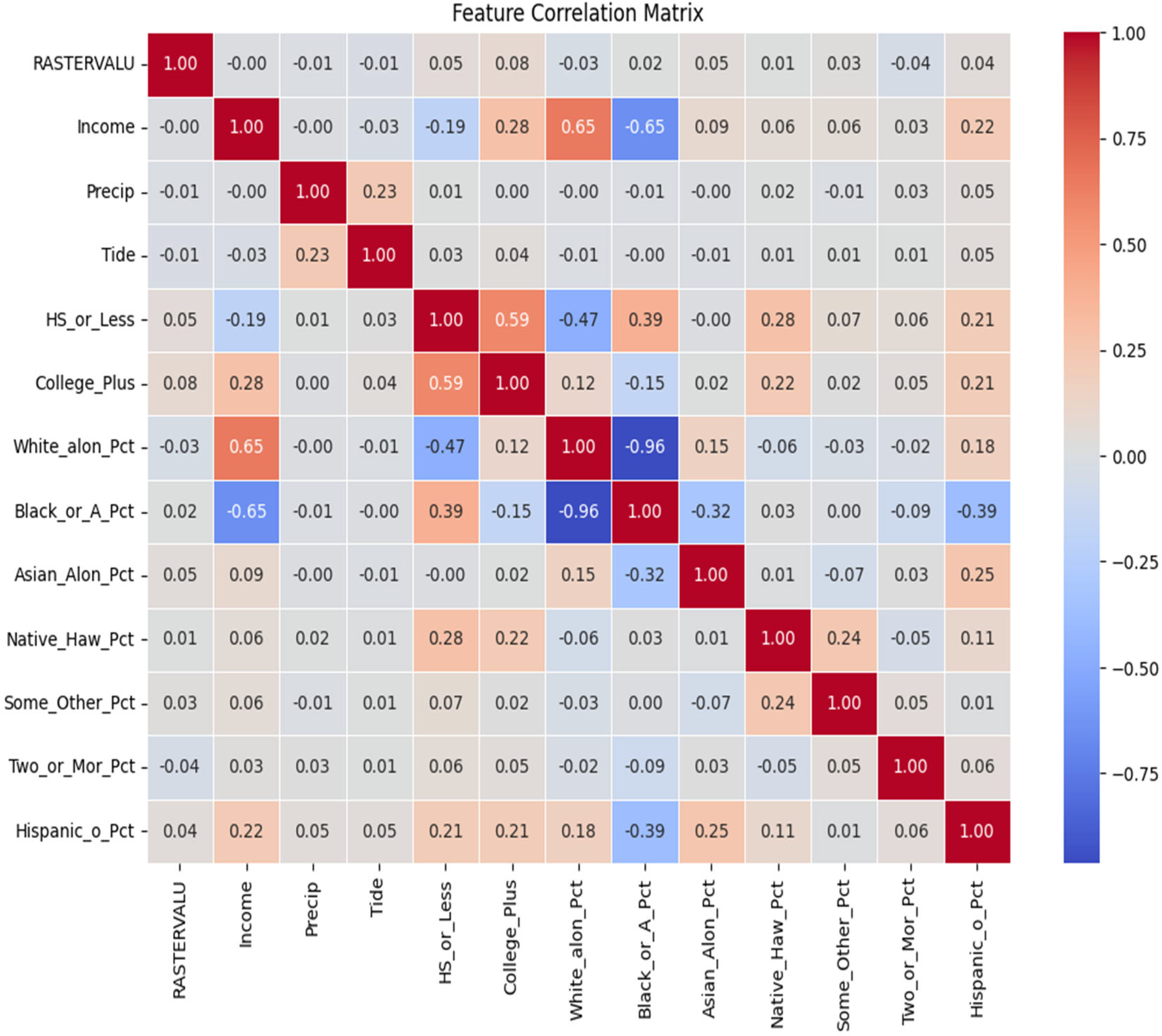
In multivariable regression analyses, some explanatory variables may be highly intercorrelated, termed multicollinearity. Multicollinearity can lead to unreliable coefficient estimates and other incorrect regression analysis results [50]. A correlation matrix (shown in Figure 2) and Variance Inflation Factor (VIF) analysis were conducted to assess multicollinearity in the explanatory variables used in this study (see Table 1). Before performing the correlation analysis, features were scaled using the standardization method, adjusting feature values by subtracting the mean and dividing by the standard deviation. Multicollinearity is determined by a VIF value of 5 to 10. Strong correlations were observed between socioeconomic variables but were strongest between the percentage of Black (Black_or_A_Pct) and the percentage of White (White_alon_Pct) variables (correlation = −0.96). Kim [50] recommends the exclusion of multicollinear variables for the development of a reliable regression model; for this reason, the percentage of White residents was removed from the model to mitigate impacts to model reliability from multicollinearity.

2.3. Building the Logistic Regression Classification Model

A logistic regression model was developed to predict the occurrence of 311 flood reports. The explanatory variables used for predicting flood stoppage service requests were socioeconomic, meteorological-oceanic, and physical environmental factors.
The explanatory variables (X) and the response variable (y) were separated and then split into test-train sets using Scikit-learn’s train_test_split function. This split randomly selected 80% of the rows (i.e., observations) as a training set and 20% as a test set (test_size = 0.2). Since the explanatory variables vary in magnitude, feature scaling was applied using standardization to ensure fair coefficient selection and reduce bias in feature importance. As shown in Equation (2) below, each feature was transformed by subtracting its mean ( μ ) and dividing by its standard deviation ( σ ). Feature scaling was performed post-splitting to prevent information leakage, which could compromise model results.
X = X μ σ
Since the dataset contained only reported occurrences, synthetic “No Report” observations were generated by randomly assigning 2–5 coordinates to “No Report” dates. Pseudo-absence generation techniques for generating presence-absence data have been utilized in environmental and ecological studies and have demonstrated improved model performance [57]. This resulted in slightly balanced classes where reports comprised 42.10% flood reporting. To account for the remaining class imbalance during model training, class weights were applied using Scikit-learn’s compute_class_weight function with the “balanced” setting. This method automatically adjusts weights inversely proportional to class frequencies, assigning more importance to underrepresented classes (i.e., the “Report” class) to reduce bias. Specifically, each class weight is computed as the total number of samples divided by the product of the number of classes and the number of samples in that class. This approach helps ensure that the model does not favor the majority class during classification.
The logistic regression model was built using Scikit-learn. Scikit-learn’s logistic regression function implements a ridge ( l 2 ) regularization, which shrinks coefficients toward zero by adding a penalty term to the loss function (see the objective function in Equation (3) below). The penalty is defined as the regularization strength, λ, multiplied by the square of the Euclidean norm of the coefficients (Equation (5)) [58,59,60]. Moreover, it can mitigate the impacts of multicollinearity on regression analysis. While measures were taken to exclude or aggregate highly correlated explanatory variables, some multicollinearity may persist [50]:
J X , y , β = y X β 2 2 + λ β 2 2
L X , y , β = y X β 2 2
P e n a l t y   t e r m = λ β 2 2
where 2 is the l 2 Euclidean norm, X is the matrix of feature variables, y is the response variable, β is the vector of coefficients associated with the features, J is the objective function, and L is the loss function.
The ridge regularization method attempts to reduce variance in regression coefficients, with large regularization strengths resulting in highly biased estimators that tend toward zero [58,60]. Consequently, coefficient estimates move away from where their unbiased ordinary least squares (OLS) estimates would be, thus making the standard error and p-values not particularly meaningful [61,62]. In other words, ridge regularization improves model numerical stability at the expense of interpretability (see SciKit Learn documentation on linear models). Consequently, 95% confidence intervals were estimated using bootstrapping as an inference of estimator significance.
Model performance was evaluated using K-fold cross-validation (k = 5 folds on the training set) and the following classification performance metrics: accuracy, precision, recall, F1-score, and receiver operating characteristic (ROC) area under the curve (AUC); Youden’s index J, a performance metric that helps define the optimal decision threshold to maximize specificity and sensitivity, was utilized to select a decision threshold that would optimize ROC AUC score [63]. The importance of explanatory variables was examined through permutation feature importance. Introduced by Breiman [64] for tree-based models, this approach for identifying critical features extends to a broad range of applications. The method works by randomly permuting each explanatory variable in order to break its natural relationship with the target variable and rerunning the model. This is repeated M times as designated by the modeler. The model classification for each run is compared with the true class label, and the output of permutation-based feature importance is the percent increase in the misclassification rate. Breiman warned that redundant variables (i.e., highly correlated variables) may not produce any decrease in the error rate because their information may be encoded in other variables. Consequently, feature importances may be under- or overestimated. To address this problem, VIFs and correlation coefficients were analyzed as part of data preprocessing, as described earlier. Additionally, variables were aggregated or excluded to reduce such impacts on the regression analysis and model inference.

3. Results

3.1. Logistic Regression Model Coefficients and Statistical Significance

The model coefficients of the logistic regression model for flood reports are shown in Table 2 below, along with their respective 95% confidence intervals computed using bootstrapping. The average k-fold cross-validation score (k = 5, ROC AUC scoring) was 0.8, indicating a well-performing, stable model. Precipitation (βPrecip = 11.592099) has the coefficient with the largest magnitude, followed by tide (βTide = 0.110156) and topographic wetness index (βRASTERVALU = −0.075085), the three statistically significant predictors (α = 0.05). However, because regularization is performed when fitting the logistic regression, coefficient magnitudes and significance must be evaluated alongside other metrics to understand their importance in the model predictions.

3.2. Model Performance Metrics

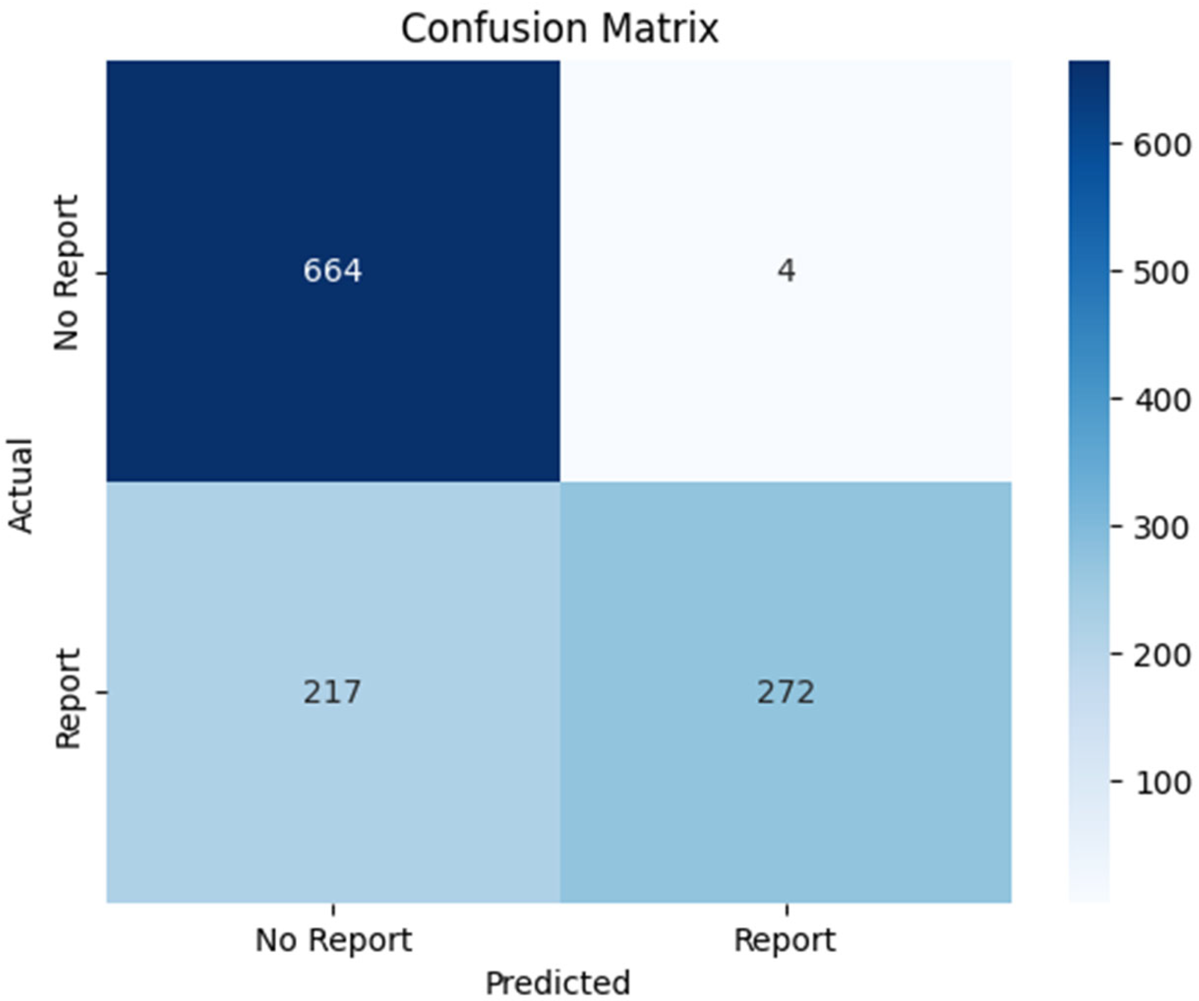
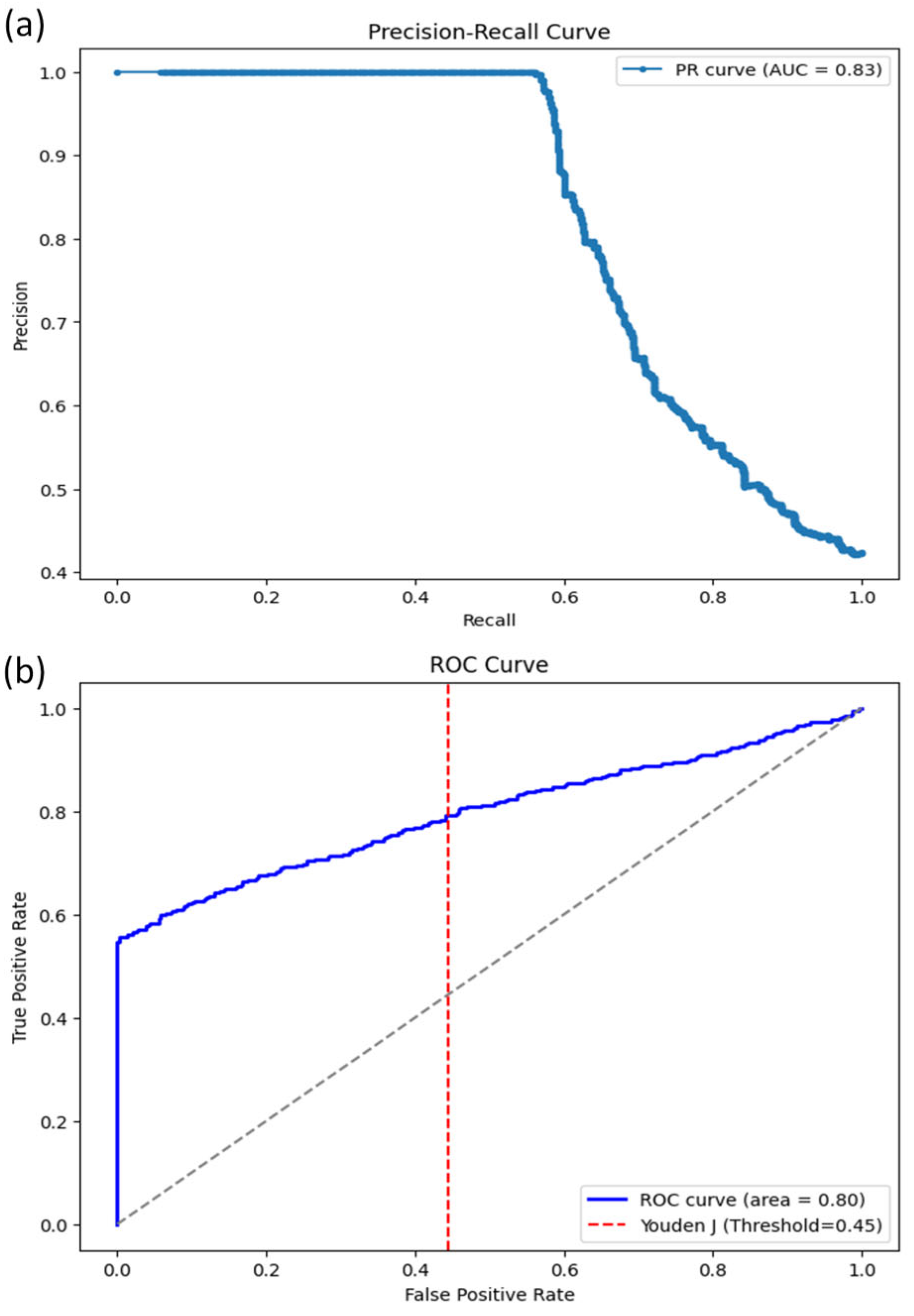
The confusion matrix in Figure 3 below compares the logistic regression model’s predicted No Report (Class 0) and Report (Class 1) classes against the actual class values. Using the decision threshold of 0.445 determined by Youden’s index, J, the model is very good at correctly predicting Class 0 observations. However, the bottom row reveals that the model is biased toward Class 0, predicting this class 217 times when the actual value was Class 1. The precision value of 0.75 for Class 0 (see Table 3) indicates that the model is falsely predicting no reports for observations where flood reports were made. However, the recall of nearly 1.0 for Class 0 indicates that the model is predicting almost all of the no-reports observations correctly. For Class 1, the model has few false positives (precision = 0.99) but often misses predicting reporting observations (recall = 0.56). Because the F1-scores, which capture the balance between precision and recall, for both classes, are above 0.7 and the model’s accuracy is 0.81, the model is considered well-performing. The model appeared to perform well in other performance metrics, with precision-recall and ROC AUC scores of 0.83 and 0.80, respectively (Figure 4a,b).

3.3. Permutation-Based Feature Importance: Identifying Salient Predictors

To inspect the relationship between predictors and the target variable, as well as the contribution of features to the model’s predictive performance, permutation-based feature importance was performed. Permutation works by shuffling a feature’s values—reconstructing its natural relationship to the response variable—and then measures how these changes impact the model’s score. This shuffling technique is repeated a specified number of times for each feature (see Scikit-Learn’s documentation on permutation-based feature importance for more information); in this study, the number of shuffles (i.e., repeats) was set to 20. As shown in Figure 5 below, shuffling precipitation resulted in the largest decrease in the ROC-AUC performance metric in the training and test sets, with an approximate median decrease in performance of 0.27. In other words, removal of the natural relationship precipitation has with flood reports results in an ROC-AUC = 0.53; without precipitation, the model would barely outperform a random guess (AUC = 0.5).
While this finding is consistent with precipitation having the largest coefficient, other socioeconomic features are found to be as or more important than tide and TWI across both sets, including percentage of Black residents, and percentage of Hispanic residents, even though their coefficients are not statistically significant. Shuffling the percentage of Black residents reduces the AUC by nearly 0.02, while shuffling the tide and percentage of Hispanic residents decreases the AUC by ~0.01. The topographic wetness index appears minimally important in the training set (shuffling decreases the AUC by less than 0.01), and its influence is further diminished when the model is predicting on unseen data (i.e., the test set). Our findings, therefore, suggest that while the direct linear relationship of demographic variables to the log-odds of a flood report is not statistically robust, the model relies on these variables to achieve its predictive performance.

4. Discussion

4.1. Environmental Predictors of Flood Reporting

Precipitation was influential in predicting flood reports, which is consistent with expectations. Precipitation ranked highest in both coefficient magnitude and permutation-based feature importance, underscoring its explanatory power for predicting the occurrence of urban flood reports. However, the tide level was not as influential in model predictions. Accounting for about 0.01 of the AUC, the importance of tide in the model’s predictive abilities was much smaller than anticipated for a low-relief, coastal, urban environment such as Norfolk, VA.
The muted role of the topographic wetness index (TWI) in the test set suggests that environmental, terrain-based variables alone are insufficient in predicting flood reports in low-relief, urban environments. This may be the result of the prevalence of impervious cover and drainage networks in shaping flood dynamics in urban coastal landscapes like Norfolk.

4.2. Demographic Influences on Reporting Behavior

In the literature, it has been observed that locations with higher incomes and a higher proportion of non-Hispanic White and Asian residents with higher educational attainment tend to be more likely to report to 311 systems, while locations with higher minority populations are less likely to report to them [44]. Contrary to these findings, this study found that an increase in the percentage of Black residents within a census tract increased the probability of a 311 report, even while controlling for other meteorological and environmental factors. This suggests Norfolk may have better educational dissemination of 311 reporting systems to Black residents than other locations. However, for locations with larger Hispanic populations, results from this study are consistent with the literature. Kontokosta et al. [44] found English language proficiency to be influential in propensity to utilize 311 reporting systems. Reporting patterns observed in this study for predominantly Hispanic populations may reflect language barriers. The MyNorfolk Portal is not currently available in Spanish, potentially contributing to underreporting.
Examination of the raw data at the census tract level reveals that tracts with higher percentages of Black residents reported flooding at comparable, or even higher, rates than those with higher percentages of White residents. As shown in Table 4, when the total population and area of the census tracts defined by these racial groups are considered, it can be seen that census tracts with predominantly Black residents tend to have higher numbers of reports per capita and higher numbers of reports per square mile. However, because the regression model controls for environmental flood risk factors such as precipitation, tide, and topographic wetness, this pattern suggests that Black residents may be more likely to report flooding rather than simply being more likely to experience it.

4.3. Education and Income Reporting Disparities

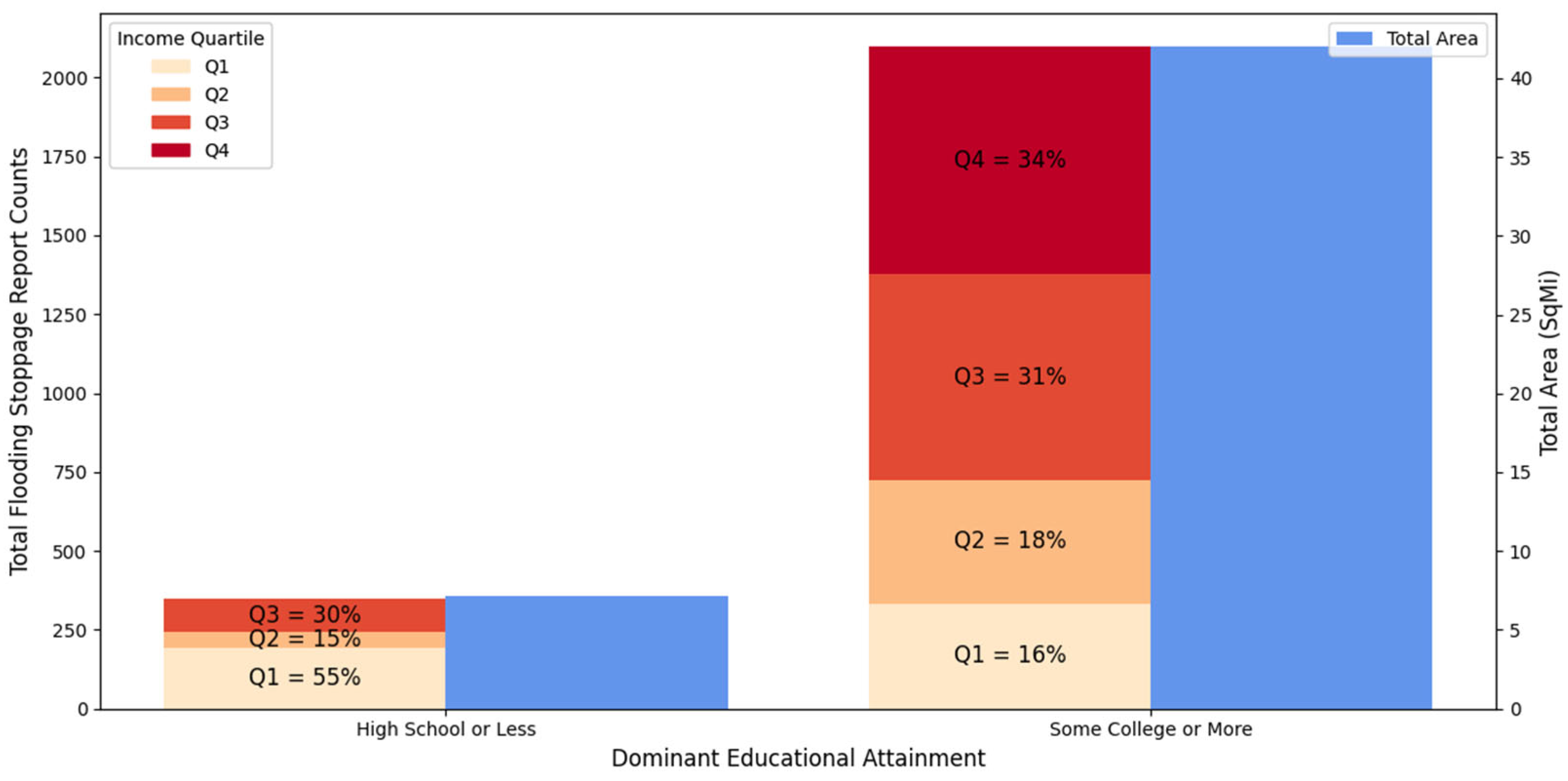
Census tracts defined by higher levels of educational attainment (some college or more) tended to have more flood reporting. It is important to note that Figure 6 and Figure 7 are descriptive figures that do not control for differences in environmental flood exposure, which may contribute to these patterns. However, the regression model in this study adjusts for environmental variables (e.g., precipitation, tide, and TWI), allowing a more accurate estimation of reporting behavior. Although the values shown in Table 4 appear to contradict previous studies that minorities underreport, the regression results affirm that Black residents are more likely to submit 311 flood reports by controlling for exposure.

5. Conclusions

This study examined the influence of climatic, physical environmental, and socioeconomic factors on the occurrence of 311 flood reports in Norfolk, Virginia. Specifically, a logistic regression model was created to predict if flooding was reported by users at a given location based on the following:
  • The 24 h cumulative precipitation on the day the flood stoppage was reported.
  • The maximum verified water level at Sewell’s Point tide station on the day the flood stoppage was reported.
  • The TWI at the location where the flood stoppage was reported.
  • The percentage of Black residents in the US Census Tract in which the flood stoppage was reported.
  • The percentage of Hispanic residents in the US Census Tract in which the flood stoppage was reported.
  • The percentage of Asian residents in the US Census Tract in which the flood stoppage was reported.
  • The percentage of residents of two or more races in the US Census Tract in which the flood stoppage was reported.
  • The Median household income for the US Census Tract in which the flood stoppage was reported.
  • The proportion of residents within the study’s defined level of educational attainment categories in the US Census Tract in which the flood stoppage was reported.
The resulting model had an accuracy of 0.81 in predicting the occurrence of a flood report with an ROC-AUC score of 0.80.
Based on a permutation feature importance model inspection of the logistic regression, precipitation was found to be the most important feature in the model, resulting in a decreased AUC of 0.27 with its influence removed. Tidal influence on model predictions was lower than anticipated for a low-relief, urban coastal environment, impacting the AUC by less than 0.01.
The crowdsourced 311 service request data provides a scalable alternative to traditional flood monitoring systems. However, reporting behaviors across demographic factors may impact the geospatial availability of this data source. This study found that the percentage of Black residents influenced the AUC by close to 0.02, with increases in the percentage of Black residents resulting in a higher likelihood of reporting. To a lesser extent, the percentage of Hispanic residents influenced the model (changing AUC by nearly 0.01), with increases in the percentage of Hispanic residents resulting in reduced reporting.
Effective stormwater management requires inclusive engagement [65]. While traditional in-person engagement strategies have improved with newer virtual formats and hybrid options [65], they can still struggle to reach civically disengaged residents, such as those with conflicting work schedules, language barriers, or distrust in institutions. The inclusion of community input through 311 data offers a valuable supplement to classical EO data sources—capturing experiential knowledge historically obtained at community engagement events. They are also immediately digitized, allowing for easy access and exploration of spatial and temporal trends for informed infrastructure investment and hazard communication.
By quantifying the influence that precipitation, tide, terrain, and socioeconomic factors have on predicting the occurrence of reports, this research adds robustness and context to crowdsourced data for identifying urban flood patterns and stormwater management needs. Future work should explore how crowdsourced data can be leveraged for real-time hydrodynamic validation (e.g., what are the lag times between event occurrence and time of reporting? And how can this be captured for hydrodynamic model validation?). Additionally, infrastructure data, demographic information on individual requests, and qualitative community feedback should be examined to understand infrastructure performance or needs and flood characteristics, such as depth. Crowdsourced observations and environmental data can enhance urban flood management strategies’ responsiveness, accuracy, and fairness.

Author Contributions

Conceptualization, N.R.L. and J.L.G.; methodology, N.R.L.; software, N.R.L.; validation, N.R.L.; formal analysis, N.R.L.; investigation, N.R.L.; resources, N.R.L.; data curation, N.R.L.; writing—original draft preparation, N.R.L.; writing—review and editing, N.R.L., J.L.G., and J.D.Q.; visualization, N.R.L.; supervision, J.L.G. and J.D.Q.; project administration, N.R.L.; funding acquisition, J.L.G. All authors have read and agreed to the published version of the manuscript.

Funding

This research was funded by the National Science Foundation (NSF), grant number 2209139.

Data Availability Statement

Data used in this study are publicly available. Flood service request data were obtained from the City of Norfolk’s MyNorfolk Portal via the city’s open data site (https://data.norfolk.gov/Government/MyNorfolk/nbyu-xjez/about_data, accessed on 2 February 2025). Socioeconomic and demographic data were retrieved from the U.S. Census Bureau’s American Community Survey (ACS) 5-year estimates: Racial demographics: 2017–2021, Table B03002, Educational attainment: 2015–2019, Table B15002, Household income: 2019–2023, Tables B19013, B19049, and B19053. Access to these tables is available via https://data.census.gov, accessed on 5 February 2025. Precipitation data were sourced from the National Center for Environmental Prediction (NCEP) Stage IV radar-based gridded precipitation product, available from the UCAR/NCAR Earth Observing Laboratory (EOL): https://data.eol.ucar.edu/dataset/21.093, accessed on 23 October 2024. Tide level data were accessed from NOAA’s Tides and Currents database for Sewell’s Point station (Station ID: 8638610): https://tidesandcurrents.noaa.gov. Topographic wetness index (TWI) was derived from a 1 m digital elevation model (DEM) of Norfolk, Virginia. The DEM was obtained from the U.S. Geological Survey (USGS) 3D Elevation Program, accessible via the National Map: https://www.usgs.gov/NationalMap, accessed on 20 October 2024. All data preprocessing and analysis steps were conducted using Python and R. Processed datasets and custom code can be made available upon reasonable request to the corresponding author.

Acknowledgments

During the preparation of this study, the author(s) used the services of the University of Virginia’s StatLab for consultation on statistical planning, preprocessing data, implementing and interpreting a statistical analysis, and data visualization. The authors have reviewed and edited the output and take full responsibility for the content of this publication.

Conflicts of Interest

The authors declare no conflicts of interest.

Abbreviations

The following abbreviations are used in this manuscript:
TWITopographic Wetness Index
SLRSea Level Rise
RSLRRelative Sea Level Rise
ROCReceiver Operator Characteristic
AUCArea Under the Curve

References

  1. NOAA National Centers for Environmental Information (NCEI). U.S. Billion-Dollar Weather and Climate Disasters; NOAA National Centers for Environmental Information (NCEI): Asheville, NC, USA, 2025. [Google Scholar] [CrossRef]
  2. Lin, N.; Kopp, R.E.; Horton, B.P.; Donnelly, J.P. Hurricane Sandy’s Flood Frequency Increasing from Year 1800 to 2100. Proc. Natl. Acad. Sci. USA 2016, 113, 12071–12075. [Google Scholar] [CrossRef]
  3. Van Oldenborgh, G.J.; Van Der Wiel, K.; Sebastian, A.; Singh, R.; Arrighi, J.; Otto, F.; Haustein, K.; Li, S.; Vecchi, G.; Cullen, H. Attribution of Extreme Rainfall from Hurricane Harvey, August 2017. Environ. Res. Lett. 2017, 12, 124009. [Google Scholar] [CrossRef]
  4. Wahl, T.; Jain, S.; Bender, J.; Meyers, S.D.; Luther, M.E. Increasing Risk of Compound Flooding from Storm Surge and Rainfall for Major US Cities. Nat. Clim. Change 2015, 5, 1093–1097. [Google Scholar] [CrossRef]
  5. Shen, Y.; Morsy, M.M.; Huxley, C.; Tahvildari, N.; Goodall, J.L. Flood Risk Assessment and Increased Resilience for Coastal Urban Watersheds under the Combined Impact of Storm Tide and Heavy Rainfall. J. Hydrol. 2019, 579, 124159. [Google Scholar] [CrossRef]
  6. Moftakhari, H.R.; AghaKouchak, A.; Sanders, B.F.; Feldman, D.L.; Sweet, W.; Matthew, R.A.; Luke, A. Increased Nuisance Flooding along the Coasts of the United States Due to Sea Level Rise: Past and Future. Geophys. Res. Lett. 2015, 42, 9846–9852. [Google Scholar] [CrossRef]
  7. Suarez, P.; Anderson, W.; Mahal, V.; Lakshmanan, T.R. Impacts of Flooding and Climate Change on Urban Transportation: A Systemwide Performance Assessment of the Boston Metro Area. Transp. Res. Part D Transp. Environ. 2005, 10, 231–244. [Google Scholar] [CrossRef]
  8. Jacobs, J.M.; Cattaneo, L.R.; Sweet, W.; Mansfield, T. Recent and Future Outlooks for Nuisance Flooding Impacts on Roadways on the U.S. East Coast. Transp. Res. Rec. J. Transp. Res. Board 2018, 2672, 1–10. [Google Scholar] [CrossRef]
  9. Nabangchang, O.; Allaire, M.; Leangcharoen, P.; Jarungrattanapong, R.; Whittington, D. Economic Costs Incurred by Households in the 2011 Greater Bangkok Flood. Water Resour. Res. 2015, 51, 58–77. [Google Scholar] [CrossRef]
  10. Cherqui, F.; Belmeziti, A.; Granger, D.; Sourdril, A.; Le Gauffre, P. Assessing Urban Potential Flooding Risk and Identifying Effective Risk-Reduction Measures. Sci. Total Environ. 2015, 514, 418–425. [Google Scholar] [CrossRef]
  11. Moftakhari, H.R.; AghaKouchak, A.; Sanders, B.F.; Matthew, R.A. Cumulative Hazard: The Case of Nuisance Flooding. Earth’s Future 2017, 5, 214–223. [Google Scholar] [CrossRef]
  12. Bedient, P.B.; Huber, W.C.; Vieux, B.E. Hydrology and Floodplain Analysis, 4th ed.; Prentice Hall: Upper Saddle River, NJ, USA, 2008; ISBN 978-0-13-174589-6. [Google Scholar]
  13. Kalyanapu, A.J.; Shankar, S.; Pardyjak, E.R.; Judi, D.R.; Burian, S.J. Assessment of GPU Computational Enhancement to a 2D Flood Model. Environ. Model. Softw. 2011, 26, 1009–1016. [Google Scholar] [CrossRef]
  14. Bates, P.D.; Anderson, M.G.; Baird, L.; Walling, D.E.; Simm, D. Modelling Floodplain Flows Using a Two-dimensional Finite Element Model. Earth Surf. Process. Landf. 1992, 17, 575–588. [Google Scholar] [CrossRef]
  15. Knebl, M.R.; Yang, Z.L.; Hutchison, K.; Maidment, D.R. Regional Scale Flood Modeling Using NEXRAD Rainfall, GIS, and HEC-HMS/ RAS: A Case Study for the San Antonio River Basin Summer 2002 Storm Event. J. Environ. Manag. 2005, 75, 325–336. [Google Scholar] [CrossRef] [PubMed]
  16. Leandro, J.; Chen, A.S.; Djordjević, S.; Savić, D.A. Comparison of 1D/1D and 1D/2D Coupled (Sewer/Surface) Hydraulic Models for Urban Flood Simulation. J. Hydraul. Eng. 2009, 135, 495–504. [Google Scholar] [CrossRef]
  17. Timbadiya, P.V.; Patel, P.L.; Porey, P.D. A 1D–2D Coupled Hydrodynamic Model for River Flood Prediction in a Coastal Urban Floodplain. J. Hydrol. Eng. 2015, 20, 05014017. [Google Scholar] [CrossRef]
  18. National Research Council. Mapping the Zone: Improving Flood Map Accuracy; National Academies Press: Washington, DC, USA, 2009; ISBN 0309130573. [Google Scholar]
  19. Lamb, R.; Crossley, M.; Waller, S. A Fast Two-Dimensional Floodplain Inundation Model. Proc. Inst. Civ. Eng.-Water Manag. 2009, 162, 363–370. [Google Scholar] [CrossRef]
  20. Yu, D. Parallelization of a Two-Dimensional Flood Inundation Model Based on Domain Decomposition. Environ. Model. Softw. 2010, 25, 935–945. [Google Scholar] [CrossRef]
  21. Morsy, M.M.; Goodall, J.L.; O’Neil, G.L.; Sadler, J.M.; Voce, D.; Hassan, G.; Huxley, C. A Cloud-Based Flood Warning System for Forecasting Impacts to Transportation Infrastructure Systems. Environ. Model. Softw. 2018, 107, 231–244. [Google Scholar] [CrossRef]
  22. Morsy, M.M.; Lerma, N.R.; Shen, Y.; Goodall, J.L.; Huxley, C.; Sadler, J.M.; Voce, D.; O’Neil, G.L.; Maghami, I.; Zahura, F.T. Impact of Geospatial Data Enhancements for Regional-Scale 2D Hydrodynamic Flood Modeling: Case Study for the Coastal Plain of Virginia. J. Hydrol. Eng. 2021, 26, 05021002. [Google Scholar] [CrossRef]
  23. National Academies of Sciences, Engineering, and Medicine; Division on Earth and Life Studies; Water Science and Technology Board; Policy and Global Affairs; Program on Risk, Resilience and Extreme Events; Committee on Urban Flooding in the United States. Framing the Challenge of Urban Flooding in the United States; National Academies Press: Washington, DC, USA, 2019; ISBN 978-0-309-48961-4. [Google Scholar]
  24. Water Resources Mission Area USGS Streamgaging Network. Available online: https://www.usgs.gov/mission-areas/water-resources/science/usgs-streamgaging-network?qt-science_center_objects=0#overview (accessed on 28 March 2024).
  25. Helmrich, A.M.; Ruddell, B.L.; Bessem, K.; Chester, M.V.; Chohan, N.; Doerry, E.; Eppinger, J.; Garcia, M.; Goodall, J.L.; Lowry, C.; et al. Opportunities for Crowdsourcing in Urban Flood Monitoring. Environ. Model. Softw. 2021, 143, 105124. [Google Scholar] [CrossRef]
  26. NOAA National Water Prediction Service The National Water Model. Available online: https://water.noaa.gov/about/nwm (accessed on 4 January 2025).
  27. Gehring, J.; Duvvuri, B.; Beighley, E. Deriving River Discharge Using Remotely Sensed Water Surface Characteristics and Satellite Altimetry in the Mississippi River Basin. Remote Sens. 2022, 14, 3541. [Google Scholar] [CrossRef]
  28. Bjerklie, D.M.; Birkett, C.M.; Jones, J.W.; Carabajal, C.; Rover, J.A.; Fulton, J.W.; Garambois, P.-A. Satellite Remote Sensing Estimation of River Discharge: Application to the Yukon River Alaska. J. Hydrol. 2018, 561, 1000–1018. [Google Scholar] [CrossRef]
  29. Ayad, M.; Li, J.; Holt, B.; Lee, C. Analysis and Classification of Stormwater and Wastewater Runoff From the Tijuana River Using Remote Sensing Imagery. Front. Environ. Sci. 2020, 8, 599030. [Google Scholar] [CrossRef]
  30. Tarpanelli, A.; Mondini, A.C.; Camici, S. Effectiveness of Sentinel-1 and Sentinel-2 for Flood Detection Assessment in Europe. In Proceedings of the EGU Natural Hazards and Earth System Sciences Discussions, Vienna, Austria, 23–27 May 2022; EGU: Vienna, Austria, 2022. [Google Scholar]
  31. Kordelas, G.; Manakos, I.; Aragonés, D.; Díaz-Delgado, R.; Bustamante, J. Fast and Automatic Data-Driven Thresholding for Inundation Mapping with Sentinel-2 Data. Remote Sens. 2018, 10, 910. [Google Scholar] [CrossRef]
  32. Vanderhoof, M.K.; Alexander, L.; Christensen, J.; Solvik, K.; Nieuwlandt, P.; Sagehorn, M. High-Frequency Time Series Comparison of Sentinel-1 and Sentinel-2 Satellites for Mapping Open and Vegetated Water across the United States (2017–2021). Remote Sens. Environ. 2023, 288, 113498. [Google Scholar] [CrossRef]
  33. Shen, X.; Anagnostou, E.N.; Allen, G.H.; Robert Brakenridge, G.; Kettner, A.J. Near-Real-Time Non-Obstructed Flood Inundation Mapping Using Synthetic Aperture Radar. Remote Sens. Environ. 2019, 221, 302–315. [Google Scholar] [CrossRef]
  34. Chini, M.; Pelich, R.; Pulvirenti, L.; Pierdicca, N.; Hostache, R.; Matgen, P. Sentinel-1 InSAR Coherence to Detect Floodwater in Urban Areas: Houston and Hurricane Harvey as A Test Case. Remote Sens. 2019, 11, 107. [Google Scholar] [CrossRef]
  35. Mason, D.C.; Trigg, M.; Garcia-Pintado, J.; Cloke, H.L.; Neal, J.C.; Bates, P.D. Improving the TanDEM-X Digital Elevation Model for Flood Modelling Using Flood Extents from Synthetic Aperture Radar Images. Remote Sens. Environ. 2016, 173, 15–28. [Google Scholar] [CrossRef]
  36. Li, Z.; Wang, C.; Emrich, C.T.; Guo, D. A Novel Approach to Leveraging Social Media for Rapid Flood Mapping: A Case Study of the 2015 South Carolina Floods. Cartogr. Geogr. Inf. Sci. 2017, 45, 97–110. [Google Scholar] [CrossRef]
  37. Wang, R.Q.; Mao, H.; Wang, Y.; Rae, C.; Shaw, W. Hyper-Resolution Monitoring of Urban Flooding with Social Media and Crowdsourcing Data. Comput. Geosci. 2018, 111, 139–147. [Google Scholar] [CrossRef]
  38. Ashktorab, Z.; Brown, C.; Nandi, M.; Culotta, A. Tweedr: Mining Twitter to Inform Disaster Response. In ISCRAM 2014 Conference, Proceedings of the 11th International Conference on Information Systems for Crisis Response and Management, University Park, PA, USA, 1 May 2014; Hiltz, S.R., Pfaff, M.S., Plotnick, L., Robinson, A.C., Eds.; ISCRAM: Brussels, Belgium, 2014; pp. 354–358. [Google Scholar]
  39. Praharaj, S.; Zahura, F.T.; Chen, T.D.; Shen, Y.; Zeng, L.; Goodall, J.L. Assessing Trustworthiness of Crowdsourced Flood Incident Reports Using Waze Data: A Norfolk, Virginia Case Study. Transp. Res. Rec. 2021, 2675, 650–662. [Google Scholar] [CrossRef]
  40. Safaei-Moghadam, A.; Tarboton, D.; Minsker, B. Estimating the Likelihood of Roadway Pluvial Flood Based on Crowdsourced Traffic Data and Depression-Based DEM Analysis. Nat. Hazards Earth Syst. Sci. 2023, 23, 1–19. [Google Scholar] [CrossRef]
  41. Chen, A.B.; Behl, M.; Goodall, J.L. Trust Me, My Neighbors Say It’s Raining Outside. In Proceedings of the 5th Conference on Systems for Built Environments, Shenzhen China, 7–8 November 2018; ACM: New York, NY, USA, 2018; pp. 25–28. [Google Scholar]
  42. Chen, A.B.; Goodall, J.L.; Chen, T.D.; Zhang, Z. Flood Resilience through Crowdsourced Rainfall Data Collection: Growing Engagement Faces Non-Uniform Spatial Adoption. J. Hydrol. 2022, 609, 127724. [Google Scholar] [CrossRef]
  43. Agonafir, C.; Pabon, A.R.; Lakhankar, T.; Khanbilvardi, R.; Devineni, N. Understanding New York City Street Flooding through 311 Complaints. J. Hydrol. 2022, 605, 127300. [Google Scholar] [CrossRef]
  44. Kontokosta, C.; Hong, B.; Korsberg, K. Equity in 311 Reporting: Understanding Socio-Spatial Differentials in the Propensity to Complain. arXiv 2017, arXiv:1710.02452. [Google Scholar] [CrossRef]
  45. Wang, L.; Qian, C.; Kats, P.; Kontokosta, C.; Sobolevsky, S. Structure of 311 Service Requests as a Signature of Urban Location. PLoS ONE 2017, 12, e0186314. [Google Scholar] [CrossRef]
  46. Sadler, J.M.; Goodall, J.L.; Morsy, M.M.; Spencer, K. Modeling Urban Coastal Flood Severity from Crowd-Sourced Flood Reports Using Poisson Regression and Random Forest. J. Hydrol. 2018, 559, 43–55. [Google Scholar] [CrossRef]
  47. Ponn, J.; Fox, M.S. Correlation Analysis Between Weather and 311 Service Request Volume; University of Toronto: Toronto, ON, Canada, 2017. [Google Scholar]
  48. Sweet, W.; Park, J.; Marra, J.; Zervas, C.; Gill, S. Sea Level Rise and Nuisance Flood Frequency Changes around the United States. In NOAA Technical Report NOS CO-OPS; National Oceanic and Atmospheric Administration (NOAA): Silver Spring, MD, USA, 2014. [Google Scholar]
  49. City of Norfolk MyNorfolk Data. Available online: https://data.norfolk.gov/Government/MyNorfolk/nbyu-xjez/about_data (accessed on 2 February 2025).
  50. Kim, J.H. Multicollinearity and Misleading Statistical Results. Korean J. Anesthesiol. 2019, 72, 558–569. [Google Scholar] [CrossRef]
  51. Du, J. NCEP/EMC 4KM Gridded Data (GRIB) Stage IV Data; Earth Observing Laboratory: Boulder, CO, USA, 2011. [Google Scholar]
  52. Blaney, L.; Perlinger, J.A.; Bartelt-Hunt, S.L.; Kandiah, R.; Ducoste, J.J. Another Grand Challenge: Diversity in Environmental Engineering. Environ. Eng. Sci. 2018, 35, 568–572. [Google Scholar] [CrossRef]
  53. Gold, A.C.; Brown, C.M.; Thompson, S.P.; Piehler, M.F. Inundation of Stormwater Infrastructure Is Common and Increases Risk of Flooding in Coastal Urban Areas Along the US Atlantic Coast. Earth’s Future 2022, 10, e2021EF002139. [Google Scholar] [CrossRef]
  54. Burgos, A.G.; Hamlington, B.D.; Thompson, P.R.; Ray, R.D. Future Nuisance Flooding in Norfolk, VA, From Astronomical Tides and Annual to Decadal Internal Climate Variability. Geophys. Res. Lett. 2018, 45, 12432–12439. [Google Scholar] [CrossRef]
  55. Ray, R.D.; Foster, G. Future Nuisance Flooding at Boston Caused by Astronomical Tides Alone. Earth’s Future 2016, 4, 578–587. [Google Scholar] [CrossRef]
  56. Beven, K.J.; Kirkby, M.J. A Physically Based, Variable Contributing Area Model of Basin Hydrology/Un Modèle à Base Physique de Zone d’appel Variable de l’hydrologie Du Bassin Versant. Hydrol. Sci. Bull. 1979, 24, 43–69. [Google Scholar] [CrossRef]
  57. Gastón, A.; García-Viñas, J.I. Modelling Species Distributions with Penalised Logistic Regressions: A Comparison with Maximum Entropy Models. Ecol. Modell. 2011, 222, 2037–2041. [Google Scholar] [CrossRef]
  58. Hastie, T. Ridge Regularization: An Essential Concept in Data Science. Technometrics 2020, 62, 426–433. [Google Scholar] [CrossRef]
  59. Šinkovec, H.; Heinze, G.; Blagus, R.; Geroldinger, A. To Tune or Not to Tune, a Case Study of Ridge Logistic Regression in Small or Sparse Datasets. BMC Med. Res. Methodol. 2021, 21, 199. [Google Scholar] [CrossRef]
  60. Sirimongkolkasem, T.; Drikvandi, R. On Regularisation Methods for Analysis of High Dimensional Data. Ann. Data Sci. 2019, 6, 737–763. [Google Scholar] [CrossRef]
  61. Revan Özkale, M.; Altuner, H. Bootstrap Confidence Interval of Ridge Regression in Linear Regression Model: A Comparative Study via a Simulation Study. Commun. Stat.-Theory Methods 2023, 52, 7405–7441. [Google Scholar] [CrossRef]
  62. Obenchain, R.L. Classical F-Tests and Confidence Regions for Ridge Regression. Technometrics 1977, 19, 429. [Google Scholar] [CrossRef]
  63. Berrar, D. Performance Measures for Binary Classification. In Encyclopedia of Bioinformatics and Computational Biology; Elsevier: Amsterdam, The Netherlands, 2019; pp. 546–560. [Google Scholar]
  64. Breiman, L. Random Forests. Mach. Learn. 2001, 45, 5–32. [Google Scholar] [CrossRef]
  65. Lerma, N.R.; Barnett, M.J.; Goodall, J.L.; Heydarian, A. Improving Online Community Engagement Practices for Infrastructure Decision-Making: Experiences from Stormwater Infrastructure Management in Houston, Texas, during the COVID-19 Pandemic. J. Infrastruct. Syst. 2024, 30, 05024002. [Google Scholar] [CrossRef]
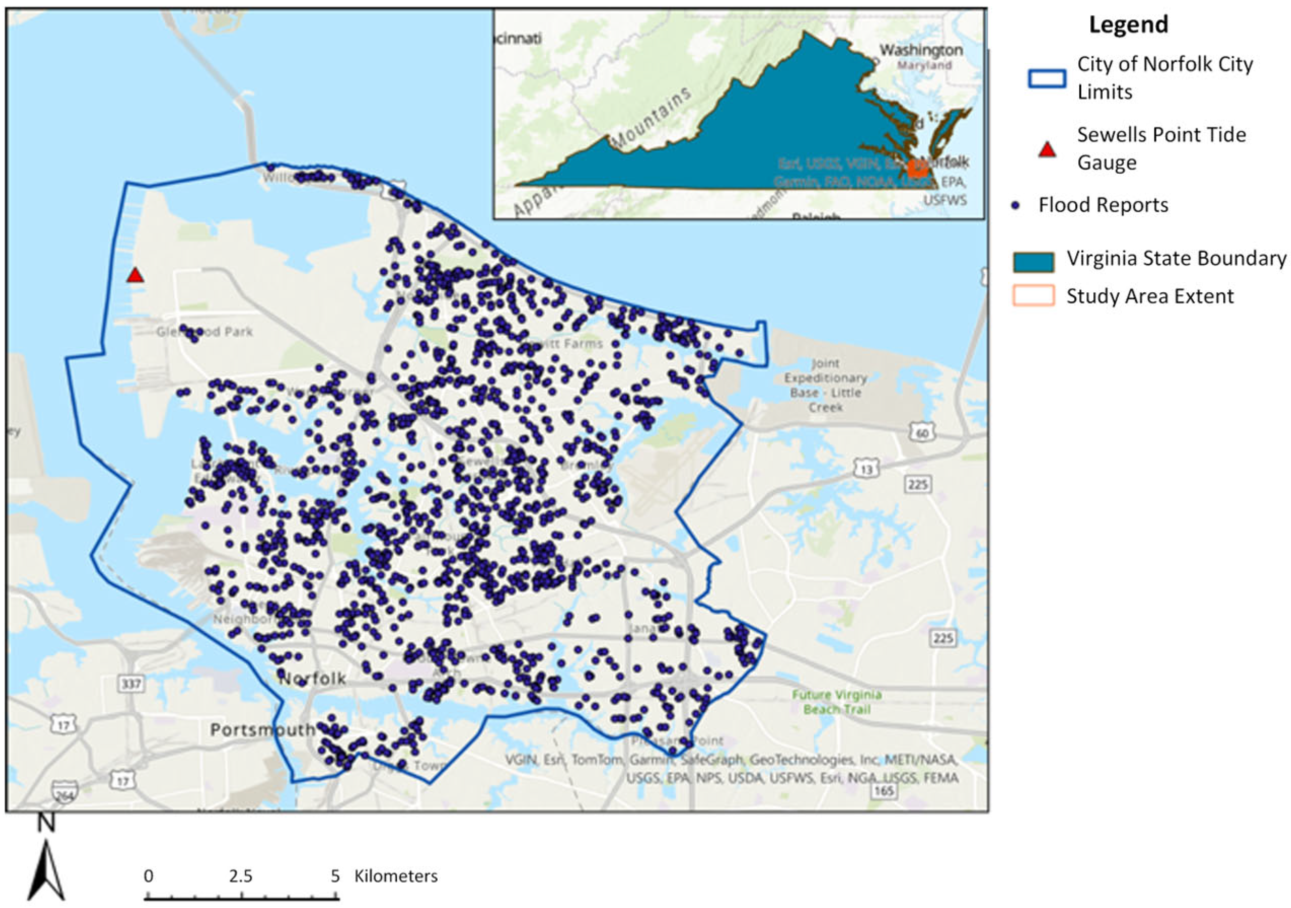
Figure 1. Map of study area—Norfolk, VA. Sewell’s Point tide gauge and locations of flood reports.
Water 17 03178 g001
Figure 2. Correlation matrix of all explanatory variables. There is a high, negative correlation between the percentage of White residents (White_alon_Pct) and the percentage of Black residents (Black_or_A_Pct), so only one variable was included to reduce multicollinearity.
Water 17 03178 g002
Figure 3. Confusion matrix of the flood reports logistic regression model (decision threshold = 0.445).
Water 17 03178 g003
Figure 4. (a) Precision-recall curve with the area under the curve at 0.83, indicating the model is performing well at identifying flood reports; (b) ROC with the area under the curve at 0.80, indicating the model is performing well at identifying flood reports. The grey dashed line in (b) denotes the reference line for a random classification performance, with an ROC AUC of 0.5.
Water 17 03178 g004
Figure 5. Permutation feature importance for (a) the training set, and (b) the test set, where the green bar represents the median, the box horizontal boundaries represent the lower and upper quartiles, and the whiskers represent the range of decreases in model performance for each explanatory variable. In both sets, precipitation is very important. To a lesser extent, the percentage of Black residents, tide level, and percentage of Hispanic residents are important for model performance.
Water 17 03178 g005
Figure 6. Flood reporting counts by predominant educational attainment compared with the total area of census tracts whose dominant educational attainment is defined by the value on the x-axis, with reports per square mile over the area bar.
Water 17 03178 g006
Figure 7. Total flooding stoppages request counts (Total Frequency) by median household income quartile (Income Quartile Ranges). The predominant racial group defining the census tracts that fall within each income quartile is visually represented, where orange represents those census tracts with predominantly White populations and blue represents census tracts with predominantly Black populations. The percentage by which each of these racially categorized census tracts makes up each quartile is shown.
Water 17 03178 g007
Table 1. Variance Inflation Factor (VIF) computed for (1) all explanatory variables, (2) the exclusion of the percentage of White residents, and (3) the exclusion of the percentage of Black residents. The variable associated with White residents (White_alon_Pct) was excluded to address multicollinearity concerns.
FeatureVariance Inflation Factor (VIF)—All VariablesVariance Inflation Factor (VIF)—Without % WhiteVariance Inflation Factor (VIF)—Without % Black
Black_or_A_Pct3123.3127053.245579
White_alon_Pct2618.2434972.720738
Hispanic_o_Pct111.1974241.5182561.256894
Asian_Alon_Pct50.2234051.2060941.098323
Two_or_Mor_Pct30.6015361.0387191.020641
HS_or_Less3.2195563.2006963.190488
Some_Other_Pct3.1635701.0847181.085332
College_Plus2.3736482.3708322.368568
Income2.0215691.9268861.939461
Native_Haw_Pct1.3258881.1772381.176874
Tide1.0627971.0627801.062781
Precip1.0584781.0582811.058283
TWI1.0165561.0165311.016545
Table 2. Feature coefficients of the logistic regression model for flood reports and bootstrapped 95% confidence intervals. * indicates the coefficient is statistically significantly different from 0 (α = 0.05).
FeatureCoefficient95% Confidence Interval
TWI−0.075085 *−0.145513, −0.005754
Income0.001985−0.101194, 0.097670
Precip11.592099 *11.119204, 12.101953
Tide0.110156 *0.031820, 0.189432
HS_or_Less−0.064699−0.187938, 0.049418
College_Plus0.020737−0.079371, 0.119930
Black_or_A_Pct0.043673−0.077009, 0.168680
Asian_Alon_Pct0.019211−0.055997, 0.092781
Two_or_Mor_Pct−0.043964−0.116751, 0.033887
Hispanic_o_Pct−0.049651−0.131265, 0.036893
Table 3. Precision, recall, F1-score, and accuracy of the logistic regression classification model for flood reporting.
ClassPrecisionRecallF1-ScoreTrue Count
00.751.000.86668
10.990.560.71489
Accuracy 0.811157
Table 4. Reports per capita and per square mile (Sq. Mi) in census tracts categorized by dominant racial group.
Reports Per CapitaReports Per Sq. Mi.
Black0.010956.2526
White0.009945.5067
Disclaimer/Publisher’s Note: The statements, opinions and data contained in all publications are solely those of the individual author(s) and contributor(s) and not of MDPI and/or the editor(s). MDPI and/or the editor(s) disclaim responsibility for any injury to people or property resulting from any ideas, methods, instructions or products referred to in the content.