Article

Combination of UAV Imagery and Deep Learning to Estimate Vegetation Height over Fluvial Sandbars

1
Institute of Geophysics Polish Academy of Sciences, 01-461 Warsaw, Poland
2
Department of Civil and Environmental Engineering, Nagoya University, Nagoya 4648603, Japan
3
Zhejiang Institute of Hydraulics and Estuary, Hangzhou 310058, China
4
Changjiang River Scientific Research Institute, Changjiang Water Resource Commission, Wuhan 430010, China
*
Authors to whom correspondence should be addressed.
Water 2025, 17(21), 3160; https://doi.org/10.3390/w17213160
Submission received: 18 September 2025 / Revised: 27 October 2025 / Accepted: 30 October 2025 / Published: 4 November 2025
(This article belongs to the Special Issue Machine Learning Applications in the Water Domain)

Abstract

Vegetation colonizing fluvial sandbars provides many noteworthy functions in river and floodplain systems, but it also influences hydrodynamic processes, mainly during flooding events. Numerical modelling is generally used to evaluate the impact of floods, but its reliability is very much connected with the accuracy of the bed and bank roughness, which is eventually altered by the presence of vegetation and its height. However, for the sake of simplicity, most models tend to ignore how the sandbar roughness varies over space and time, as a function of the local vegetation dynamics (spatial distribution and height). To determine the long-term dynamic vegetation condition using remote sensing multispectral indexes, this study leverages a deep-learning method to establish a relationship between vegetation height (h), a critical parameter for vegetation roughness estimation, and vegetation indexes (VIs) collected by an uncrewed aerial vehicle (UAV). A field campaign was performed in October 2024 covering the Baishazhou sandbar, located along a straight section of the Wuhan reach of the Changjiang River Basin, China. The results show that the R2 and RMSE between the real and predicted vegetation height by the trained Fully Connected Neural Network (FCNN) are 0.85, 1.10 m, and the relative error reaches a maximum of 17.2%, meaning that the trained FCNN model performs rather well. Despite being tested on a single case study, the workflow presented here demonstrates the opportunity to use UAVs for depicting vegetation characteristics such as height over large areas, eventually using them to inform numerical models that consider sandbar roughness.

1. Introduction

Sandbars are key geomorphic features in fluvial systems, crucial for bedload transport and sediment storage [1,2]. Formed by hydrodynamic-sedimentary interactions, they evolve dynamically with flow and sediment changes [3]. Sandbar morphology and vegetation cover serve as vital indicators of riverine dynamics and channel morphology [4,5,6], revealing spatiotemporal feedbacks between primary and secondary channels and adjacent floodplains. Highly vegetated sandbars can function similarly to riverbanks during low flow [7]. The establishment of vegetation increases surface roughness and flow resistance, which reduces floodplain conveyance capacity and elevates local water levels, thereby increasing flood risk [8]. Vegetation conditions such as height, density, and species composition further govern these hydrodynamic and sediment transport processes during floods [9]. The vegetation-induced increased resistance can distort the stage-discharge relationship, leading to higher water levels and greater flooding hazard, particularly in conveyance-sensitive, low-gradient systems [10].
In hydrodynamic models, a fundamental tool for flood prediction, risk assessment, and water resource management, surface roughness is critical to obtain accurate simulations [11,12]. However, roughness of fluvial surfaces (e.g., riverbeds, banks) is not static [12], but dynamically responds to vegetation changes. Indeed, extreme floods can rapidly alter vegetation structure and distribution [13], causing significant shifts in hydraulic characteristics and compromising predictions of water levels and inundation extents.
Predictive models that incorporate temporally variable vegetation characteristics are vital for accurately estimating changes in flow resistance over time [14]. To support such modelling efforts, robust and continuous monitoring of vegetation dynamics is indispensable. This includes tracking changes in vegetation height, density, spatial coverage, and species composition across different temporal scales, from seasonal growth cycles to rapid post-flood recovery periods. Accurate spatial and temporal data on vegetation are critical not only for capturing the interactions between flow, morphology, and ecology (i.e., hydro-morpho-biodynamic processes), but also for informing adaptive management strategies aimed at flood mitigation, habitat enhancement, and sustainable river management [15].
Previous studies have investigated the relationship between roughness and riparian vegetation via experimental methods [16,17,18,19]. All those studies concluded that vegetation characteristics significantly influence the flow structure by means of changes in roughness. Traditional field measurements of vegetation using handheld instruments [20] are increasingly supplemented by remote sensing, which offers superior spatial coverage, resolution, and efficiency [21]. Consequently, remote sensing is often preferred for characterizing vegetation before roughness calculations in practical applications. Multispectral Vegetation Indices (VIs), particularly the widely used Normalized Difference Vegetation Index (NDVI), have been established to monitor vegetation dynamics [22,23,24], differentiate vegetated areas [25], and quantify biomass [26]. Recent studies pointed out that its variant, the Green Normalized Difference Vegetation Index (GNDVI), is more effective for assessing health in dense canopies [27].
Given easier access, as well as advantages such as cost- and time-effectiveness, VIs calculated from satellite images to estimate vegetation parameters are more widely used to derive potential relationships between VIs and vegetation parameters such as vegetation height or density [28,29]. Additionally, with the advantage of having higher spatial resolution when compared with satellite images, multispectral uncrewed aerial vehicles (UAVs) have been used to obtain vegetation conditions recently [30], especially in the estimation of vegetation height [22,31,32]. Although previous studies successfully applied drones to monitor the vegetation height, most of them focused on a single plant species, while research on regions with various plants is limited. At the same time, UAVs can not only measure the vegetation height and density directly but also capture multispectral images for calculating VIs. The combination of UAVs and satellite images makes vegetation monitoring on long-time scales much easier to achieve. Specifically, after understanding how vegetation parameters can be explained by VIs determined from UAV collections, long-term vegetation parameters can be estimated from VIs derived from satellite images.
However, establishing relationships between VIs and vegetation parameters remains challenging, especially in the case of vegetation height, which is an important parameter for estimating vegetation roughness [21,33]. Fortunately, deep-learning (DL) models, with their elevated performance and ability to handle complex input-output relationships, might help address this limitation thanks to their higher prediction accuracy compared to traditional fitting methods [34]. The main applications of DL in remote sensing include image-based object detection and multimodal data fusion [35]. While classical machine learning (ML) methods like Random Forest have shown effectiveness in vegetation identification and height estimation [36,37,38], their supervised learning nature demands substantial manual annotation. To address this limitation, researchers have started exploring self-supervised and semi-supervised learning approaches [39,40,41]. For example, Du et al. [42] utilized a CNN Transformer hybrid model called NeCT Net to extract spatial features and employed a semi-supervised teacher-student framework to automatically generate pseudo labels for expanding training data. This method effectively reduces dependence on manual annotation while improving the accuracy of large-scale building height estimation. Although supervised learning approaches have demonstrated significant success in vegetation height estimation, their applications have predominantly focused on forest canopies or single crop types, with limited exploration in multi-class study areas comprising complex vegetation communities. Concurrently, while advanced DL architectures such as CNN-Transformer hybrids have achieved breakthroughs in building height estimation by integrating semi-supervised strategies, these models often entail complex structures and high computational costs. In response, this study adopts a streamlined FCNN as its core architecture to substantially simplify the training process and computational requirements while maintaining high accuracy.
Aiming to establish a relationship between vegetation height (h) and VIs (NDVI, GNDVI, Normalized Difference Red Edge Index (NDRE), Leaf Chlorophyll Index (LCI), and Optimized Soil Adjusted Vegetation Index (OSAVI), to lay the foundation for the calculation of vegetation roughness, this research analysed vegetation conditions and multispectral images of the Baishazhou middle sandbar, in the middle reaches of the Yangtze River (China), using a UAV (DJI Mavic 3 Multispectral) and employed the FCNN model for analysis. Using a reduced number of data points, the h-VIs relationship was established, eventually allowing us to extract it over time to monitor long-term variations in vegetation conditions from satellite images, therefore reducing the need for prolonged and cumbersome UAV field campaigns. By means of a specific case study, the current work proposes a workflow to determine the relationship between vegetation indexes and vegetation height, which can be applied to both UAV and satellite imagery, eventually assisting in extracting dynamic roughness to be used as a reliable input for hydrodynamic flood modelling.

2. Materials and Methods

2.1. Study Area

Located in the straight section of the Wuhan reach of the Changjiang River Basin (Figure 1), the Baishazhou (BSZ) sandbar is oriented in a northeast-southwest direction. The left branch of the sandbar serves as the main channel, and the right branch is the tributary. Formed by the sediment carried by the river water, the BSZ sandbar takes the shape of a bamboo leaf, which is typical of those whose upstream and downstream ends are pointed, while the middle section is wider, with a measured length of 2.2 km and a maximum width of 0.3 km during the dry season.
The BSZ sandbar is located in a region characterized by a subtropical monsoon climate, with average yearly temperature and precipitation around 17.7 °C and 1204.50 mm, respectively [43]. The annual average runoff and sediment from 1990 to 2020 recorded by the Hankou Hydrological station, which is 20 km downstream of the BSZ sandbar, are 7012.73 × 108 m3 and 1.94 × 10⁸ t, respectively [44].
Since the Baishazhou Bridge spans the middle of the sandbar (Figure 1B), the area above the middle part of the sandbar is designated as a no-fly zone. Therefore, for this research, two small areas on either side of the bridge were selected as study areas to obtain the images (Figure 1A).

2.2. UAV Data Collecting and Processing

2.2.1. UAV Information and Data Collection

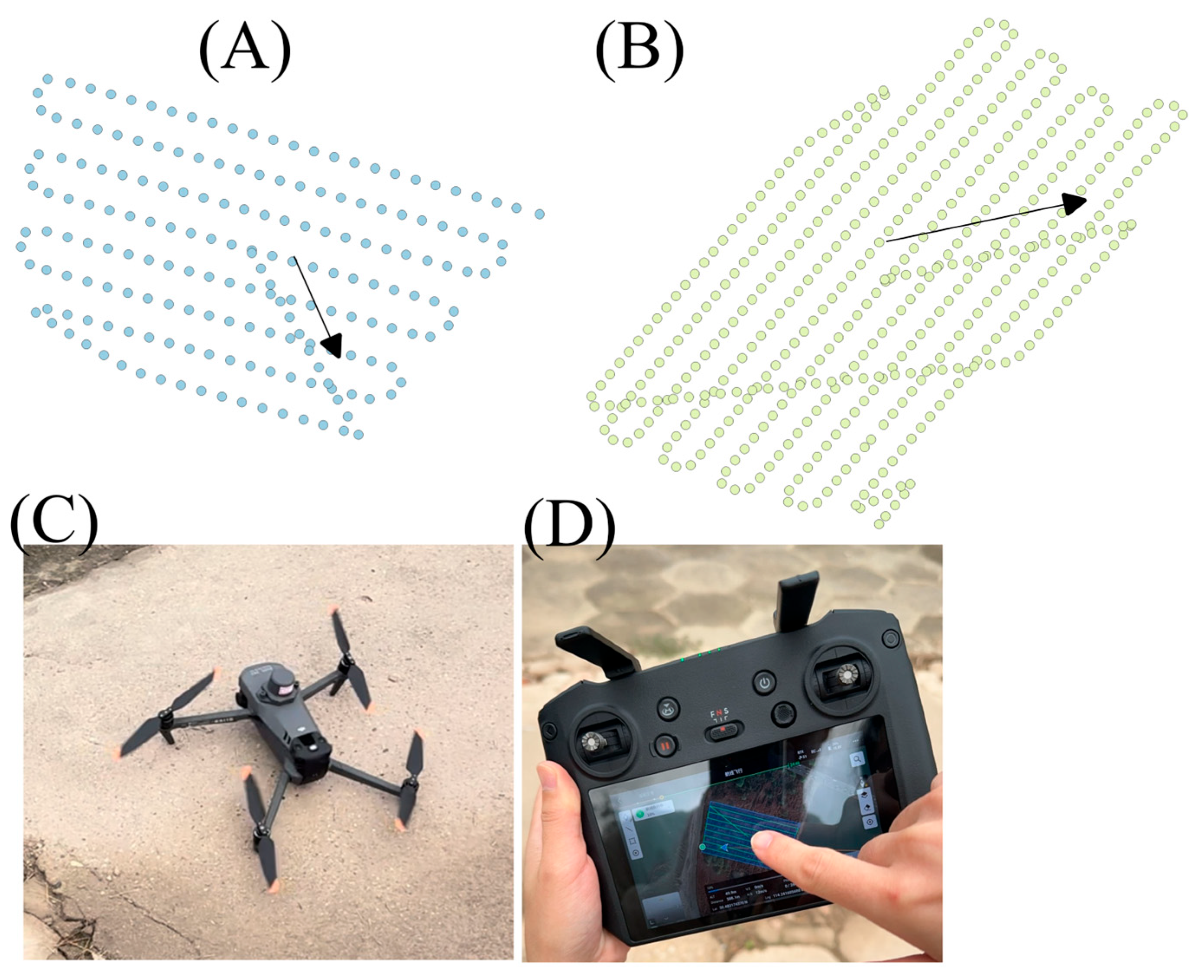
A DJI Mavic 3 Multispectral (M3M) (SZ DJI Technology Co., Ltd., Shenzhen, China) equipped with a natural colour camera and a four-band multispectral sensor (Figure 2C,D) was used to obtain spectral information of the sandbar (green band: 560 nm; red band: 650 nm; red edge: 730 nm; near-infrared: 860 nm) [45]. The flight path (Figure 2A,B) was pre-programmed using the DJI Pilot software v10.00.06.02 with a flying height of approx. 60 m. The drone flight took place during the Autumn season, on 12 October 2024, a sunny day.

2.2.2. Calculation of Vegetation Indexes (VIs) and Estimation of Vegetation Height

VIs calculated by differences between several spectral bands are designed to highlight vegetation properties (such as canopy biomass, absorbed radiation, and chlorophyll content) and vegetation’s vigour [46]. Five VIs (NDVI, GNDVI, NDRE, LCI, and OSAVI), derived using the reflectance of vegetation in the visible, red edge, and near-infrared bands, are selected under consideration of the spectral bands available in multispectral UAV and Sentinel-2 imagery.
Among all the VIs, NDVI is the most commonly used index for quantitatively measuring vegetation conditions [47,48]. As shown in Equation (1), NDVI is calculated as the ratio of the difference and the sum of reflectance values in the near-infrared (NIR) and red bands (R). Therefore, NDVI values vary between −1 and 1, with higher values for more densely vegetated and healthy areas.
N D V I = N I R R N I R + R
Compared with NDVI, which reflects vegetation health through the levels of chlorophyll detected in the leaves, the green normalized difference vegetation index (GNDVI), introduced by Gitelson et al. [49] and defined in Equation (2), is more suitable for monitoring crop yield in the late growing season because the green band (G) can cover a broader range of chlorophyll than the red band adopted in NDVI [50,51].
G N D V I = N I R G N I R + G
NDRE, defined as Equation (3), is similar to NDVI but is more sensitive to chlorophyll content in denser vegetation [52]. It calculates based on reflectance in the near-infrared (NIR) and red edge (RE) bands. When the NDVI is no longer sufficiently sensitive to changes in the plant biomass in the later stages of plant growth, NDRE plays an important role.
N D R E = N I R R E N I R + R E
The LCI, which uses the near-infrared (NIR), red edge (RE), and green (G) bands (Equation (4)), provides more accurate chlorophyll content information than the NDRE index [53].
L C I = N I R R E N I R + G
OSAVI considers the substrate type during vegetation condition analysis, reducing the influence of bare soil and enabling image correction where soil is visible between vegetation [54]. The OSAVI is defined following Equation (5), where C is a calibration constant that minimizes the influence of soil and takes the value of 0.16 [55].
O S A V I = N I R R N I R + R + C
The NDVI, GNDVI, LCI, NDRE, and OSAVI layers are overlapped in QGIS 3.40.11. The value of each grid is treated as a group of data for training the FCNN model, with a total of 78,520,680 data points.
The Digital Surface Model (DSM) and the Digital Elevation Model (DEM) are constructed by means of the DJI Terra software, and their difference is used to estimate vegetation heights. The DSM contains the height information of all objects on the Earth’s surface, while the DEM represents the elevation of the bare ground surface. The difference between the two eliminates the influence of the underlying ground elevation, retaining only the height characteristics of surface objects such as vegetation [56]. Therefore, the vegetation height is estimated by the difference between the plant surface (DSM) and the terrain (DEM). Both DSM and DEM are processed based on the drone imagery by the DJI Terra software, and the DEM is also pre-processed to filter out all the vegetation [57], ensuring an accurate estimation of the vegetation height.
To ensure the measurement accuracy of the DJI M3M (SZ DJI Technology Co., Ltd., Shenzhen, China) with real-time kinematic (RTK) equipment, it has been verified prior to the drone’s release. The results show that the output images can meet the requirements of 1:500 large-scale mapping accuracy, and the absolute/relative positioning error did not surpass 0.05 m/0.15 m in the horizontal and vertical directions, respectively [58]. Previous studies also found that the errors of DEM and DSM created from the imagery collected by DJI M3M are very low, generally around 1.5 cm [59,60,61]. The DEM and DSM collected from the drone imagery are, therefore, considered reliable for the scope of the current investigation.

2.3. Model Architecture of FCNN

The flowchart for data processing and constructing the FCNN model is shown in Figure 3, and comprises five main parts, described below in detail.
  • Step 1
The first step is organizing the original data. The h, NDVI, and GNDVI values of every pixel are listed in three columns in Excel as the original dataset.
  • Step 2
Secondly, the dataset is split into two subsets: 70% of the data is used for training the model, and the rest (30%) is for validation, to ensure that the evaluation of the model’s performance on unseen data is reliable. This splitting was selected based on literature evidence that investigated the predictive capability of machine learning models, proving that the 70/30 one presented the best performance among all tested models [62].
The training set is randomly selected from the original data, while the rest of the data is used to validate the model, and thereafter is defined as the test set. It is worth reminding here that the present application focused on developing a workflow, so no independent datasets were used for testing.
  • Step 3
Structuring and training the FCNN model is the third step.
The structure of the model layers is as follows:
1. Input data layer. The input layers include a dataset consisting of vegetation height values, NDVI values, and GNDVI. The h, NDVI, and GNDVI of each grid are regarded as a group of data. The dataset is composed of data groups from each grid.
2. Hidden layers. The hidden layers are able to capture the underlying features and patterns in the data and learn hidden variables to enhance prediction capabilities [63]. Two fully connected layers (with every layer having 10 neurons) expand the feature space and enable the network to learn complex representations. Aiming to introduce non-linearity and allow the network to learn non-linear patterns efficiently [64], the rectified linear unit has been introduced.
In this study, ReLU (Equation (6)), one of the most widely used activation functions [65,66], serves as the activation function for each fully connected layer.
R e L U x = max 0 , x
where x indicates the input to the neuron [67].
3. Output layers. A single neuron is used to output a continuous value. The activation function of the output layer is a linear function, allowing the output to be directly mapped from the learned features.
  • Step 4
Fourthly, the test set is imposed as the input for the trained model.
  • Step 5
Finally, the performance of the estimations is evaluated by calculating the coefficient of determination (R2) [68] and root mean squared error (RMSE) [36] between the calculated and the measured data. As a significant index for evaluating the model’s performance, R2 is able to quantify the model’s ability to explain the variance in the data [68], with a higher R2 indicating better model performance.

3. Results

3.1. Monitoring of Vegetation Height

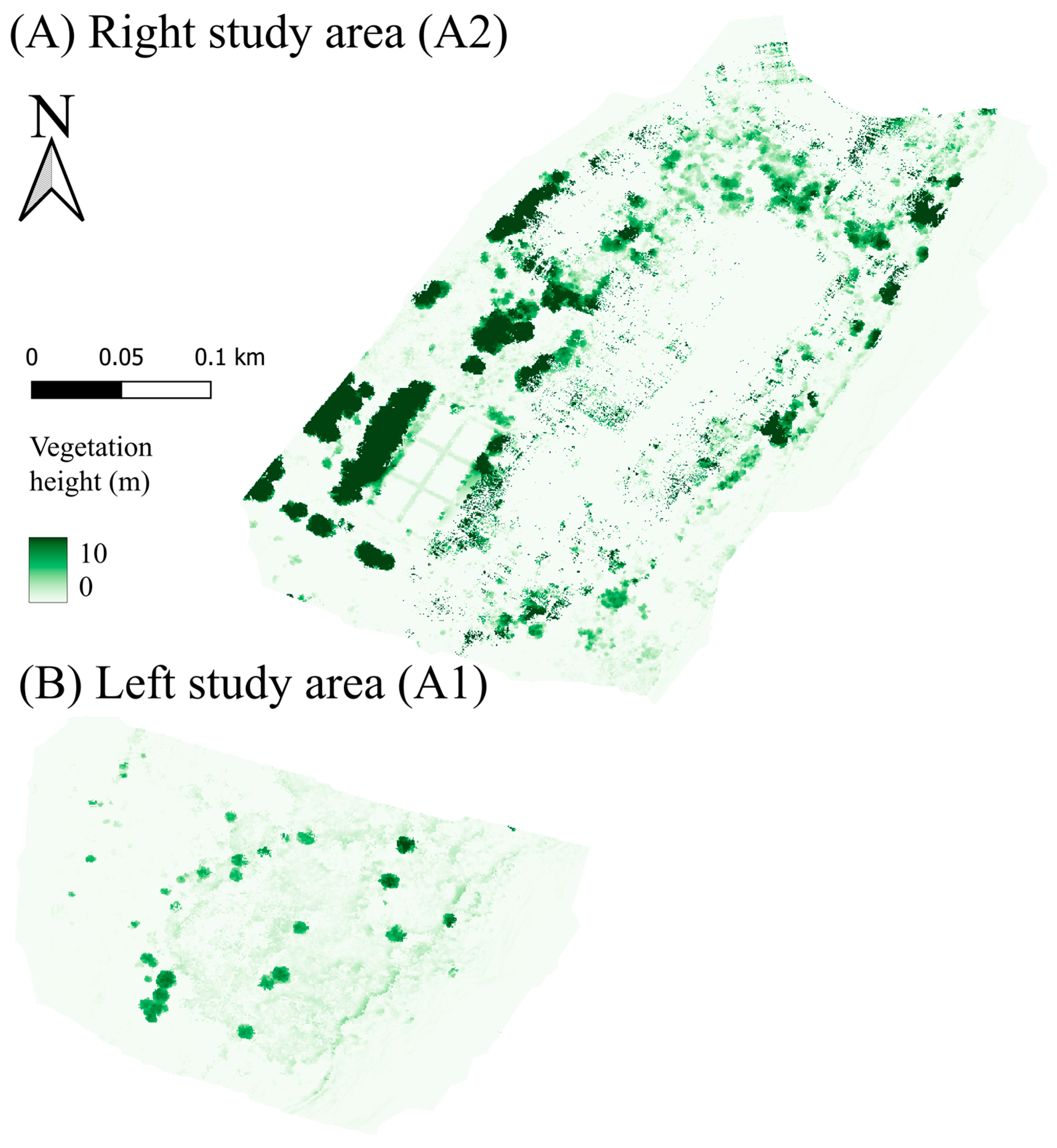
The distribution of the vegetation height of the two study areas estimated by DSM minus the vegetation-filtered DEM is illustrated in Figure 4. It can be noticed that the vegetation height of both A1 and A2 ranges from 0 to 10 m, with an average height of 0.81 m in A1 and 3.38 m in A2. The average vegetation height of the two areas is 2.10 m.
High plants in A1 are mainly isolated points without any obvious distribution pattern, while those in A2 are patchily distributed throughout the region, showing no clear distribution pattern. Vegetation along the boundary of A1 is generally characterized by low values. Regarding the boundary of A2, the condition is quite different, as there is a large area of high vegetation along the left boundary of A2 and lower vegetation along the right boundary.
Table 1 reports the statistics of the monitored vegetation height. As visible, most of the plants are smaller than 2 m, covering around 95.35%, 81.98%, and 85.36% of areas A1, A2, and the whole area, respectively. For A1, height is inversely proportional to quantity, that is, the higher the plants are, the lower the proportion of vegetation. In area A2, vegetation heights greater than 8 m rank second in frequency with a value of 8.02%, and there is a decreasing trend in vegetation height within the 2–8 m range. For the whole area, the trend is similar to that of A2, since A2 is bigger than A1: 85.36% of vegetation is less than 2 m, while 6.08% of vegetation is bigger than 8 m.

3.2. Spatial Distribution of NDVI and GNDVI

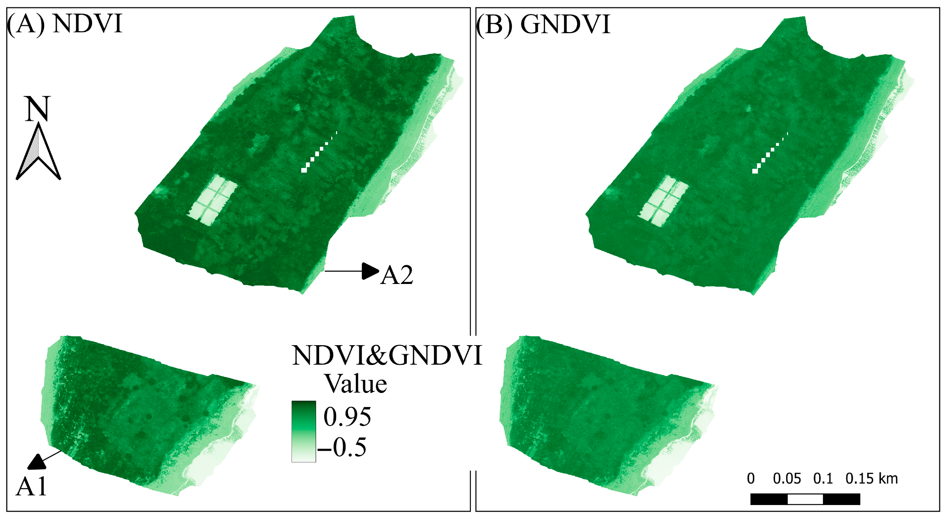
The distributions of the NDVI and GNDVI estimated by the aerial images from the UAV are illustrated in Figure 5. It is found that the GNDVI value is slightly lower overall with respect to NDVI. The average NDVI and GNDVI of A1 are 0.62 and 0.59, respectively, and those of A2 are 0.71 and 0.64, respectively, meaning that the vegetation of A2 seems healthier than that of A1.
Moreover, the variability in the spatial distribution of NDVI values for A1 is greater than that of its GNDVI. The NDVI in A1 has a trend, with higher values at the border and lower in the middle, while the trend of GNDVI is not obvious. When it comes to the variability in the spatial distribution of NDVI and GNDVI values for area A2, they are more similar.

3.3. Linear and Polynomial Regression Based Vegetation Height Prediction

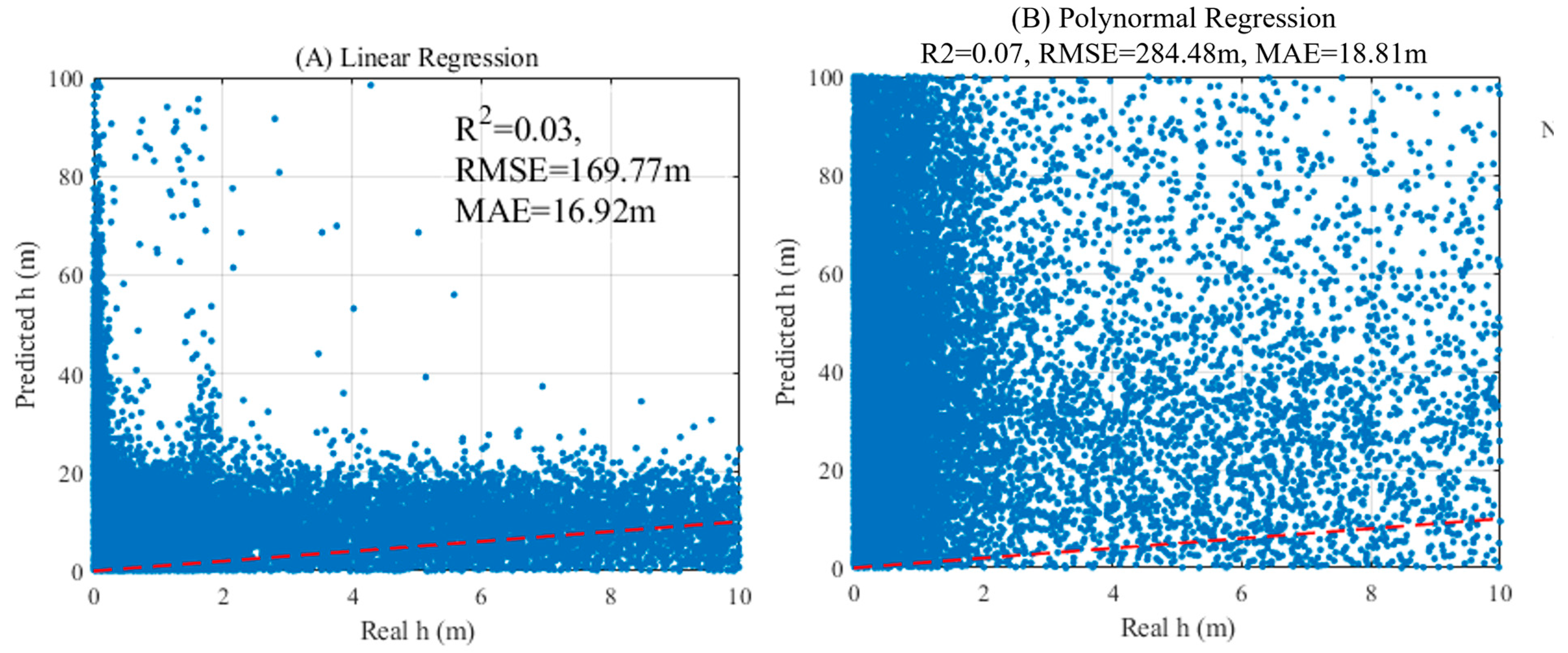
The vegetation height estimated by the linear regression model is shown in Figure 6A, the results revealed a weak relationship between the predictor variables (NDVI, GNDVI, LCI, NDRE, and OSAVI) and vegetation height, with a training R2 of 0.03, root mean square error (RMSE) of 169.77 m, and a mean absolute error (MAE) of 16.92 m. The linear regression equation derived in the present case study is h = 3.9879 + (−25.2569 × NDVI) + (−22.5722 × GNDVI) + (200.4915 × LCI) + (−155.0283 × NDRE) + (−1.1886 × OSAVI). It is possible to note that the large coefficient values suggest potential overfitting and numerical instability. In summary, the linear regression model demonstrated limited performance in estimating vegetation height from multispectral indices.
The polynomial regression model showed modest improvement over linear regression but still exhibited inadequate performance (Figure 6B), with training results displaying an R2 of 0.07, RMSE of 284.48 m, and MAE of 18.01 m. Although the polynomial model incorporated interaction terms and quadratic features, expanding the feature space from 5 to 20 dimensions, the minimal improvement in R2 and the increase in MAE suggest that increasing model complexity alone cannot adequately address the underlying estimation challenges.

3.4. Deep Learning-Based Vegetation Height Prediction

The above reported limitations in using linear and polynomial regression models ask for more complex approaches, such as the use of deep learning.
70% of the vegetation height h, NDVI, and GNDVI values estimated from the UAV images are used to train the FCNN model, where h is the dependent variable and NDVI and GNDVI are the independent variables. The other 30% of the NDVI and GNDVI values are imported into the trained model to predict h. The predictions are then compared to the original vegetation height to verify the performance of the trained model.
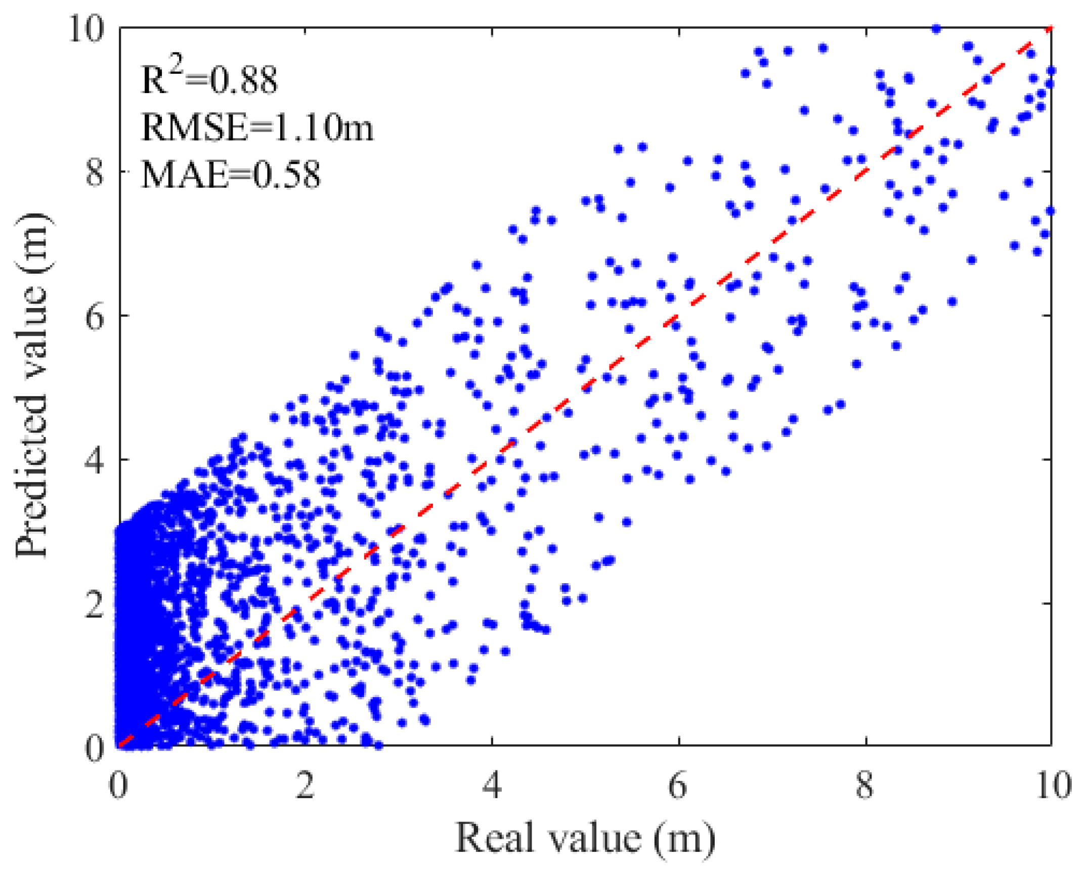
The calibration results (Figure 7) demonstrate exceptionally strong model performance, with a coefficient of determination (R2) of 0.88, indicating that the model explains 88% of the variance in vegetation height. This represents a remarkable improvement over previous modeling attempts and confirms the effectiveness of the current approach. The model’s error metrics, with an RMSE of 1.10 m and a MAE of 0.58 m, fall within an acceptable range for vegetation height estimation applications. The fact that MAE is substantially lower than RMSE suggests a generally well-behaved error distribution without excessive outliers.

4. Discussion

In recent years, the frequency and intensity of flood events have increased significantly, largely driven by the ongoing impacts of climate change [69]. These heightened flood hazards are causing considerable disruptions to both human settlements and natural ecosystems, necessitating urgent and innovative approaches to flood management [70]. The growing unpredictability and severity of extreme weather events, such as intense rainfall and prolonged storms, underscore the importance of developing not only more effective flood mitigation strategies but also robust resilience frameworks capable of adapting to future climate scenarios. This includes integrating dynamic environmental variables, such as the behaviour of aquatic and riparian vegetation, which have been shown to exert a profound influence on hydrodynamic processes during flood events. In fact, the role of vegetation in shaping the flow dynamics of rivers and floodplains is becoming increasingly recognised as a critical factor in flood risk assessments [71]. Research on dynamic vegetation during high-flow conditions is gaining particular attention in the academic and practical realms of hydrology and geomorphology. As vegetation can grow and change rapidly in response to seasonal variations, extreme weather events, and restoration efforts, its influence on flood dynamics is not static, but rather highly variable and context-dependent. Vegetation can serve as a natural barrier to floodwaters, slowing their advance and reducing the overall volume of water that may inundate surrounding areas. However, this same vegetation can also impede drainage and exacerbate localised flooding if it is too dense or improperly distributed. Therefore, understanding how vegetation interacts with both the riverine environment and the flow dynamics during different flood stages is crucial to accurately modelling flood events and their impacts [72], as well as to develop sustainable flood management practices that are resilient to the growing challenges posed by climate change [73].
Past investigations have shown that accurately describing the involved processes and quantifying the influence of in-channel and riparian vegetation on bed roughness is very challenging. Generally, the vegetation roughness is calculated by formulas such as the Baptist approach, based on a Chézy formulation [74], and the Järvelä approach, which expands the previous method by accounting for submerged or emergent, flexible, and woody vegetation [75]. Moving from these approaches, Box et al. [76] proposed additional formulas accounting for the presence of leaves in both submerged and emergent conditions, showing how they can be implemented in numerical modelling. However, for all existing methods, how to estimate each vegetation parameter in real conditions is still a challenge, in particular in estimating the effective vegetation height influencing the flow field in rivers and streams, as well as their dynamics over time and space.
An answer to this knowledge gap could come from the combination of UAV imagery, orbital remote sensing, vegetation indices, and ML techniques [77]. To establish the relationship between vegetation height and VIs, this study conducted field measurements at the BSZ sandbar, a middle sandbar in the Middle Changjiang River, by using a UAV. Given the limited effectiveness of the initially tried linear and quadratic regression models, which yielded R2 values around 0.3, a basic deep learning model, namely the FCNN model, was subsequently employed. After splitting the data into training and testing sets (70/30), we used NDVI, GNDVI, LCI, NDRE, and OSAVI (calculated from Sentinel-2 satellite imagery) as features in the trained model to estimate vegetation height. The model’s performance metrics were R2 = 0.27, RMSE = 0.97 m, and MAE = 0.31 m. Despite the mediocre but acceptable metrics of the FCNN model, it is worth noting that the results presented here are influenced by the season, as field measurements were carried out in October (Autumn), which is not the best season for vegetation conditions. Though the vegetation height may not change a lot, the vegetation is not as green as in the Summer, causing the NDVI value to be rather low. This is likely the reason why the GNDVI value is lower than the NDVI. Although the results are suboptimal, they are not irrelevant for height estimation. Since this study utilizes only a single vegetation image for model training, it cannot fully capture the vegetation growth cycle. Furthermore, the sampling date was in autumn, which is not the ideal season for data collection. The achieved R2 of 0.27 suggests that incorporating multi-temporal data in the future could enable the model to better simulate vegetation height.
It should be highlighted that the outcomes presented here are based on a reduced dataset, and therefore, more field measurements should be conducted in the future in different seasons to improve the trained model, to effectively describe the vegetation seasonality [47]. The presented relationship between vegetation indexes and vegetation height should be further tested, as the current results might be influenced by vegetation characteristics such as photosynthetic activity and density of the visible leaves. At the same time, it is worth reminding that the overall workflow proposed here is disconnected from the vegetation seasonality and characteristics, and could therefore be replicated under different vegetation conditions, aiming to cover a wider range of vegetative stages and species.
Furthermore, the estimation of the vegetation height obtained from UAV data is also affected by uncertainties. Although the drone used in this study is equipped with an Real-Time Kinematic (RTK) module, whose measurement error has been proved can be controlled within 1–2 cm [78], and the DSM-DEM approach used to calculate the vegetation height has been tested by many researchers and defined as reliable [79,80,81,82], errors still exist since the DEM and DSM has potential uncertainties connected to the spatial resolution. Thus, some small vegetation may be missed from the removal procedure when filtering the vegetation cover on the DEM, leading to a slight overestimation of the vegetation height. To address this point, in future measurement campaigns, it is planned to employ a UAV with light detection and ranging (LiDAR) to extract the vegetation height directly to minimize errors [83]. At the same time, advanced methodologies and reference tests to reduce uncertainties [84] will also be considered.
Meanwhile, more VIs will be introduced to train the deep-learning model to consider more vegetation conditions and types. For example, in this case, the dominant vegetation type is (high) grass, with shrubs and trees sparsely distributed in the central sandbar. Therefore, the models are trained only by NDVI and GNDVI and without classifying vegetation types. The Enhanced Vegetation Index (EVI) will be introduced in future studies to account for more complicated vegetation conditions. In fact, this index was developed as a standard satellite vegetation product for the Terra and Aqua Moderate Resolution Imaging Spectroradiometers (MODIS), and provides improved sensitivity in high biomass regions while minimizing soil and atmosphere influences through a decoupling of the canopy background signal [85].
It is also worth remembering that traditional regression methods, such as linear regression, perform poorly in fitting the relationship between vegetation height and VIs (namely, NDVI and GNDVI). To address this limitation, more advanced approaches such as DL models (convolutional neural network (CNN), recurrent neural network (RNN), and long short-term memory network (LSTM)) should be used. Though the FCNN model performs rather well in this application, a wider range of DL models will also be tested in the future to corroborate the presented outcomes and eventually improve them, aiming to provide a more robust estimation of vegetation height from VIs that could be extrapolated to other areas.
The influence of the spatial resolution of multispectral images on estimating vegetation height from VIs is another focus for future research. Sensitivity analyses of spatial resolution to the DL model trained by using UAV-acquired vegetation height data and VIs are also planned, considering images of varying spatial resolution (e.g., 0.5 m, 1 m, 5 m, 10 m, etc.) that will be captured by UAVs to investigate how spatial resolution affects building the relationship between vegetation heights and VIs.
Despite current limitations, the present study highlighted the opportunity to use UAVs for estimating vegetation height and consequent roughness. This demonstrates that VIs calculated from remote sensing (UAVs currently and their combination with satellite imagery in the future) could be used to estimate vegetation characteristics, assuming an adequate spatial resolution.

5. Conclusions

The vegetation parameters, especially the vegetation height, are essential for estimating dynamic vegetation roughness. Though the VIs can be obtained from both satellite and UAV images, the vegetation height is hard to extract from satellite images, given the relatively low spatial resolution and the infrequent revisit time. Focusing on a sandbar in the Middle Changjiang River (China), a relationship between vegetation height and VIs collected by the UAV field measurement is built here, taking advantage of an FCNN model. The results find that there is a very strong positive correlation between the predictions and the real values, and around 85% of the variation in the vegetation height can be explained by the trained model, showing that the vegetation height estimated by the trained FCNN model is reliable. Therefore, in the next stage, the VIs derived from satellite images can be used as inputs to the trained FCNN model to estimate vegetation height, eventually enlarging the study area and extending the observation period.
The results presented here contribute to the development of repeatable, cost-effective, and fine-scale vegetation monitoring strategies based on UAV flights, supported by photogrammetry.

Author Contributions

Conceptualization, Y.G.; methodology, Y.G.; field measurement: Y.G., Y.Z. and R.Z.; software, Y.G.; validation, Y.G. and M.N.; formal analysis, Y.G.; investigation, Y.G.; data curation, Y.G.; writing—original draft preparation, Y.G. and M.N.; writing—review and editing, Y.G., M.N., Y.Z., R.Z. and W.D.; visualization, Y.G.; supervision, M.N.; project administration, M.N.; funding acquisition, M.N. All authors have read and agreed to the published version of the manuscript.

Funding

This research was funded by the National Natural Science Foundation of Joint Fund for Changjiang River Water Science Research, Project number U2340215 and by the National Science Centre Poland–call PRELUDIUM BIS-3, Grant Number 2021/43/O/ST10/00539. The work of Y.G. and M.N. is partially supported by a subsidy from the Polish Ministry of Education and Science for the Institute of Geophysics Polish Academy of Sciences.

Data Availability Statement

The data used in the study are available at https://zenodo.org/records/15834789 (accessed on 1 May 2025).

Conflicts of Interest

The authors declare no conflicts of interest.

References

  1. Sweeney, M.R.; Fischer, B.; Wermers, K.; Cowman, T. Eolian and Fluvial Modification of Missouri River Sandbars Deposited by the 2011 Flood, USA. Geomorphology 2019, 327, 111–125. [Google Scholar] [CrossRef]
  2. Stucker, J.H.; Buhl, D.A.; Sherfy, M.H. Emergent Sandbar Construction for Least Terns on the Missouri River: Effects on Forage Fishes in Shallow-Water Habitats. River Res. Appl. 2012, 28, 1254–1265. [Google Scholar] [CrossRef]
  3. Seki, S.; Moteki, D.; Yasuda, H. Novel Hypothesis on the Occurrence of Sandbars. Phys. Fluids 2023, 35, 106611. [Google Scholar] [CrossRef]
  4. Hu, Y.; Zhou, J.; Deng, J.; Li, Y.; Yang, C.; Li, D. River Bars and Vegetation Dynamics in Response to Upstream Damming: A Case Study of the Middle Yangtze River. Remote Sens. 2023, 15, 2324. [Google Scholar] [CrossRef]
  5. Heidari, N.; Yagci, O.; Aksel, M. Midchannel Islands in Lowland River Corridors and Their Impacts on Flow Structure and Morphology: A Numerical Based Conceptual Analysis. Ecol. Eng. 2021, 173, 106419. [Google Scholar] [CrossRef]
  6. Rood, S.B.; Goater, L.A.; Gill, K.M.; Braatne, J.H. Sand and Sandbar Willow: A Feedback Loop Amplifies Environmental Sensitivity at the Riparian Interface. Oecologia 2011, 165, 31–40. [Google Scholar] [CrossRef]
  7. Nagata, T.; Watanabe, Y.; Yasuda, H.; Ito, A. Development of a Meandering Channel Caused by the Planform Shape of the River Bank. Earth Surf. Dyn. 2014, 2, 255–270. [Google Scholar] [CrossRef]
  8. van Iersel, W.; Straatsma, M.; Addink, E.; Middelkoop, H. Monitoring Height and Greenness of Non-Woody Floodplain Vegetation with UAV Time Series. ISPRS J. Photogramm. Remote Sens. 2018, 141, 112–123. [Google Scholar] [CrossRef]
  9. Nones, M.; Di Silvio, G. Modeling of River Width Variations Based on Hydrological, Morphological, and Biological Dynamics. J. Hydraul. Eng. 2016, 142, 04016012. [Google Scholar] [CrossRef]
  10. Kiss, T.; Nagy, J.; Fehérváry, I.; Vaszkó, C. (Mis) Management of Floodplain Vegetation: The Effect of Invasive Species on Vegetation Roughness and Flood Levels. Sci. Total Environ. 2019, 686, 931–945. [Google Scholar] [CrossRef]
  11. De Doncker, L.; Troch, P.; Verhoeven, R.; Bal, K.; Meire, P.; Quintelier, J. Determination of the Manning Roughness Coefficient Influenced by Vegetation in the River Aa and Biebrza River. Environ. Fluid Mech. 2009, 9, 549–567. [Google Scholar] [CrossRef]
  12. Chen, Y.; Cao, F.; Cheng, W.; Liu, B.; Yu, P. Real-Time Correction of Channel-Bed Roughness and Water Level in River Network Hydrodynamic Modeling for Accurate Forecasting. Sci. Rep. 2023, 13, 20660. [Google Scholar] [CrossRef] [PubMed]
  13. Ferreira, D.M.; Fernandes, C.V.S.; Kaviski, E.; Bleninger, T. Calibration of River Hydrodynamic Models: Analysis from the Dynamic Component in Roughness Coefficients. J. Hydrol. 2021, 598, 126136. [Google Scholar] [CrossRef]
  14. Augustijn, D.C.M.; Huthoff, F.; Van Velzen, E.H. Comparison of Vegetation Roughness Descriptions. In Proceedings of the River Flow 2008: 4th International Conference on Fluvial Hydraulics, Izmir, Turkey, 3–5 September 2008; pp. 343–350. [Google Scholar]
  15. Latella, M.; Notti, D.; Baldo, M.; Giordan, D.; Camporeale, C. Short-Term Biogeomorphology of a Gravel-Bed River: Integrating Remote Sensing with Hydraulic Modelling and Field Analysis. Earth Surf. Process. Landforms 2024, 49, 1156–1178. [Google Scholar] [CrossRef]
  16. Kiss, T.; Fehérváry, I. Increased Riparian Vegetation Density and Its Effect on Flow Conditions. Sustainability 2023, 15, 12615. [Google Scholar] [CrossRef]
  17. Signorile, A.; Saracino, R.; Dani, A.; Rillo Migliorini Giovannini, M.; Preti, F. Riparian Vegetation Surveys for Roughness Estimation. Ecol. Eng. 2024, 209, 107414. [Google Scholar] [CrossRef]
  18. Wang, J.; Zhang, Z. Evaluating Riparian Vegetation Roughness Computation Methods Integrated within HEC-RAS. J. Hydraul. Eng. 2019, 145, 04019020. [Google Scholar] [CrossRef]
  19. Rillo Migliorini Giovannini, M.; Dani, A.; Saracino, R.; Signorile, A.; Preti, F. Hydraulic Roughness Estimation Induced by Riparian Vegetation in Tuscany Rivers for Management Purposes. Lect. Notes Civ. Eng. 2023, 337, 169–179. [Google Scholar] [CrossRef]
  20. Chen, S.; McDermid, G.J.; Castilla, G.; Linke, J. Measuring Vegetation Height in Linear Disturbances in the Boreal Forest with UAV Photogrammetry. Remote Sens. 2017, 9, 1257. [Google Scholar] [CrossRef]
  21. Chaulagain, S.; Stone, M.C.; Dombroski, D.; Gillihan, T.; Chen, L.; Zhang, S. An Investigation into Remote Sensing Techniques and Field Observations to Model Hydraulic Roughness from Riparian Vegetation. River Res. Appl. 2022, 38, 1730–1745. [Google Scholar] [CrossRef]
  22. Lu, J.; Cheng, D.; Geng, C.; Zhang, Z.; Xiang, Y.; Hu, T. Combining Plant Height, Canopy Coverage and Vegetation Index from UAV-Based RGB Images to Estimate Leaf Nitrogen Concentration of Summer Maize. Biosyst. Eng. 2021, 202, 42–54. [Google Scholar] [CrossRef]
  23. Gao, L.; Wang, X.; Johnson, B.A.; Tian, Q.; Wang, Y.; Verrelst, J.; Mu, X.; Gu, X. Remote Sensing Algorithms for Estimation of Fractional Vegetation Cover Using Pure Vegetation Index Values: A Review. ISPRS J. Photogramm. Remote Sens. 2020, 159, 364–377. [Google Scholar] [CrossRef] [PubMed]
  24. Zhang, J.; Qiu, X.; Wu, Y.; Zhu, Y.; Cao, Q.; Liu, X.; Cao, W. Combining Texture, Color, and Vegetation Indices from Fixed-Wing UAS Imagery to Estimate Wheat Growth Parameters Using Multivariate Regression Methods. Comput. Electron. Agric. 2021, 185, 106138. [Google Scholar] [CrossRef]
  25. Leroux, L.; Baron, C.; Zoungrana, B.; Traore, S.B.; Lo Seen, D.; Begue, A. Crop Monitoring Using Vegetation and Thermal Indices for Yield Estimates: Case Study of a Rainfed Cereal in Semi-Arid West Africa. IEEE J. Sel. Top. Appl. Earth Obs. Remote Sens. 2016, 9, 347–362. [Google Scholar] [CrossRef]
  26. Amani, S.; Shafizadeh-Moghadam, H. A Review of Machine Learning Models and Influential Factors for Estimating Evapotranspiration Using Remote Sensing and Ground-Based Data. Agric. Water Manag. 2023, 284, 108324. [Google Scholar] [CrossRef]
  27. Berzéki, M.; Kozma-Bognár, V.; Berke, J. Examination of Vegetation Indices Based on Multitemporal Drone Images; Gradus: Düsseldorf, Germany, 2023; Volume 10. [Google Scholar] [CrossRef]
  28. Sun, H.; Wang, X.; Fan, D.; Sun, O.J. Contrasting Vegetation Response to Climate Change between Two Monsoon Regions in Southwest China: The Roles of Climate Condition and Vegetation Height. Sci. Total Environ. 2022, 802, 149643. [Google Scholar] [CrossRef]
  29. Payero, J.O.; Neale, C.M.U.; Wright, J.L. Comparison of Eleven Vegetation Indices for Estimating Plant Height of Alfalfa and Grass. Appl. Eng. Agric. 2004, 20, 385–393. [Google Scholar] [CrossRef]
  30. Kalinowska, M.B.; Västilä, K.; Nones, M.; Kiczko, A.; Karamuz, E.; Brandyk, A.; Kozioł, A.; Krukowski, M. Influence of Vegetation Maintenance on Flow and Mixing: Case Study Comparing Fully Cut with High-Coverage Conditions. Hydrol. Earth Syst. Sci. 2023, 27, 953–968. [Google Scholar] [CrossRef]
  31. Boucher, P.B.; Hockridge, E.G.; Singh, J.; Davies, A.B. Flying High: Sampling Savanna Vegetation with UAV-Lidar. Methods Ecol. Evol. 2023, 14, 1668–1686. [Google Scholar] [CrossRef]
  32. Luo, S.; Liu, W.; Zhang, Y.; Wang, C.; Xi, X.; Nie, S.; Ma, D.; Lin, Y.; Zhou, G. Maize and Soybean Heights Estimation from Unmanned Aerial Vehicle (UAV) LiDAR Data. Comput. Electron. Agric. 2021, 182, 106005. [Google Scholar] [CrossRef]
  33. Prior, E.M.; Aquilina, C.A.; Czuba, J.A.; Pingel, T.J.; Hession, W.C. Estimating Floodplain Vegetative Roughness Using Drone-Based Laser Scanning and Structure from Motion Photogrammetry. Remote Sens. 2021, 13, 2616. [Google Scholar] [CrossRef]
  34. Nguyen, H.D.; Van, C.P.; Do, A.D. Application of Hybrid Model-Based Deep Learning and Swarm-based Optimizers for Flood Susceptibility Prediction in Binh Dinh Province, Vietnam. Earth Sci. Inform. 2023, 16, 1173–1193. [Google Scholar] [CrossRef]
  35. Gui, S.; Song, S.; Qin, R. Remote Sensing Object Detection in the Deep Learning Era—A Review. Remote Sens. 2024, 16, 327. [Google Scholar] [CrossRef]
  36. Wang, W.; Tang, J.; Zhang, N.; Xu, X.; Zhang, A.; Wang, Y.; Li, K.; Wang, Y. Vegetation Height Estimation Based on Machine Learning Model Driven by Multi-Source Data in Eurasian Temperate Grassland. Ecol. Indic. 2025, 170, 113013. [Google Scholar] [CrossRef]
  37. Luo, H.; Ou, G.; Yue, C.; Zhu, B.; Wu, Y.; Zhang, X.; Lu, C.; Tang, J. A Framework for Montane Forest Canopy Height Estimation via Integrating Deep Learning and Multi-Source Remote Sensing Data. Int. J. Appl. Earth Obs. Geoinf. 2025, 138, 104474. [Google Scholar] [CrossRef]
  38. Bhandari, K.; Srinet, R.; Nandy, S. Forest Height and Aboveground Biomass Mapping by Synergistic Use of GEDI and Sentinel Data Using Random Forest Algorithm in the Indian Himalayan Region. J. Indian Soc. Remote Sens. 2024, 52, 857–869. [Google Scholar] [CrossRef]
  39. Dersch, S.; Schöttl, A.; Krzystek, P.; Heurich, M. Semi-Supervised Multi-Class Tree Crown Delineation Using Aerial Multispectral Imagery and Lidar Data. ISPRS J. Photogramm. Remote Sens. 2024, 216, 154–167. [Google Scholar] [CrossRef]
  40. Yang, R.; Chen, M.; Lu, X.; He, Y.; Li, Y.; Xu, M.; Li, M.; Huang, W.; Liu, F. Integrating UAV Remote Sensing and Semi-Supervised Learning for Early-Stage Maize Seedling Monitoring and Geolocation. Plant Phenomics 2025, 7, 100011. [Google Scholar] [CrossRef]
  41. Nyamekye, C.; Appiah, L.B.; Arthur, R.; Osei, G.; Ofosu, S.A.; Kwofie, S.; Ghansah, B.; Bryniok, D. Comparing Supervised and Semi-Supervised Machine Learning Methods for Mapping Aquatic Weeds, as Biomass Resource from High-Resolution UAV Images. Remote Sens. Earth Syst. Sci. 2024, 7, 206–217. [Google Scholar] [CrossRef]
  42. Du, S.; Liu, H.; Xing, J.; Zhang, X.; Zhang, J.; Guan, X.; Du, S. Estimating Individual Building Heights by Integrating Spaceborne LiDAR and Multisource Remote Sensing Data: A CNN–Transformer Model and a Semi-Supervised Sample Augmentation Approach. IEEE Trans. Geosci. Remote Sens. 2025, 63, 5406719. [Google Scholar] [CrossRef]
  43. Jiang, Y.; Chen, X.F.; Yang, X.J. A Study on Changes of Aquatic Plants in East Lake of Wuhan Using 1990–2020 Landsat Images. Chin. J. Plant Ecol. 2022, 46, 1551–1561. [Google Scholar] [CrossRef]
  44. Wang, X.; Li, Z.; Ma, J.; Bai, K. Differential Scour of Two Mid-Channel Bars in Wuhan Reach of the Middle Yangtze River. J. Chang. River Sci. Res. Inst. 2024, 41, 18–27. [Google Scholar] [CrossRef]
  45. Fraser, B.T.; Robinov, L.; Davidson, W.; O’Connor, S.; Congalton, R.G. A Comparison of Unpiloted Aerial System Hardware and Software for Surveying Fine-Scale Oak Health in Oak–Pine Forests. Forests 2024, 15, 706. [Google Scholar] [CrossRef]
  46. Gutierrez-Rodriguez, M.; Escalante-Estrada, J.A.; Rodriguez-Gonzalez, M.T. Canopy Reflectance, Stomatal Conductance, and Yield of Phaseolus vulgaris L. and Phaseolus coccinues L. Under Saline Field Conditions. Int. J. Agric. Biol. 2005, 7, 491–494. [Google Scholar]
  47. Boothroyd, R.J.; Nones, M.; Guerrero, M. Deriving Planform Morphology and Vegetation Coverage from Remote Sensing to Support River Management Applications. Front. Environ. Sci. 2021, 9, 657354. [Google Scholar] [CrossRef]
  48. Rouse, J.W., Jr.; Haas, R.H.; Schell, J.A.; Deering, D.W. Monitoring Vegetation Systems in the Great Plains with ERTS. In Proceedings of the NASA Goddard Space Flight Center 3d ERTS-1 Symposium, Washington, DC, USA, 1 January 1974; Volume 1. Section A. [Google Scholar]
  49. Gitelson, A.A.; Kaufman, Y.J.; Merzlyak, M.N. Use of a Green Channel in Remote Sensing of Global Vegetation from EOS-MODIS. Remote Sens. Environ. 1996, 58, 289–298. [Google Scholar] [CrossRef]
  50. Barati, S.; Rayegani, B.; Saati, M.; Sharifi, A.; Nasri, M. Comparison the Accuracies of Different Spectral Indices for Estimation of Vegetation Cover Fraction in Sparse Vegetated Areas. Egypt. J. Remote Sens. Sp. Sci. 2011, 14, 49–56. [Google Scholar] [CrossRef]
  51. Allawai, M.F.; Ahmed, B.A. Using Remote Sensing and GIS in Measuring Vegetation Cover Change from Satellite Imagery in Mosul City, North of Iraq. IOP Conf. Ser. Mater. Sci. Eng. 2020, 757, 012062. [Google Scholar] [CrossRef]
  52. Karpiński, P.; Kocira, S.; Karpiński, P.; Kocira, S. Possibilities of Using a Multispectral Camera to Assess the Effects of Biostimulant Application in Soybean Cultivation. Sensors 2025, 25, 3464. [Google Scholar] [CrossRef]
  53. Bak, H.-J.; Kim, E.-J.; Lee, J.-H.; Chang, S.; Kwon, D.; Im, W.-J.; Kim, D.-H.; Lee, I.-H.; Lee, M.-J.; Hwang, W.-H.; et al. Canopy-Level Rice Yield and Yield Component Estimation Using NIR-Based Vegetation Indices. Agriculture 2025, 15, 594. [Google Scholar] [CrossRef]
  54. Steven, M.D. The Sensitivity of the OSAVI Vegetation Index to Observational Parameters. Remote Sens. Environ. 1998, 63, 49–60. [Google Scholar] [CrossRef]
  55. Rondeaux, G.; Steven, M.; Baret, F. Optimization of Soil-Adjusted Vegetation Indices. Remote Sens. Environ. 1996, 55, 95–107. [Google Scholar] [CrossRef]
  56. Popescu, S.C.; Zhao, K. A Voxel-Based Lidar Method for Estimating Crown Base Height for Deciduous and Pine Trees. Remote Sens. Environ. 2008, 112, 767–781. [Google Scholar] [CrossRef]
  57. DJI. DJI Terra-User Manual; v4.3; DJI: Shenzhen, China, 2024. [Google Scholar]
  58. Tan, C.; Chen, Z.; Liao, A.; Chen, Z.; Zeng, X. Accuracy Assessment of Mavic 3 Industrial UAV Based on DJI Terra and Pix4Dmapper. In Proceedings of the Fifth International Conference on Geology, Mapping, and Remote Sensing, Wuhan, China, 10 July 2024; SPIE: Bellingham, WA, USA; Volume 13223, pp. 498–504. [Google Scholar] [CrossRef]
  59. Carp, A. Measuring Accuracy of the DJI Mavic 3 Enterprise RTK Using DroneDeploy Photogrammetry; DroneDeploy: San Francisco, CA, USA, 2023. [Google Scholar]
  60. Wang, M.; Li, H.; Liu, Y.; Li, H. Multi-Source DEM Vertical Accuracy Evaluation of Taklimakan Desert Hinterland Based on ICESat-2 ATL08 and UAV Data. Remote Sens. 2025, 17, 1807. [Google Scholar] [CrossRef]
  61. Liu, J.; Wang, W.; Li, J.; Mustafa, G.; Su, X.; Nian, Y.; Ma, Q.; Zhen, F.; Wang, W.; Li, X. UAV Remote Sensing Technology for Wheat Growth Monitoring in Precision Agriculture: Comparison of Data Quality and Growth Parameter Inversion. Agronomy 2025, 15, 159. [Google Scholar] [CrossRef]
  62. Nguyen, Q.H.; Ly, H.B.; Ho, L.S.; Al-Ansari, N.; Van Le, H.; Tran, V.Q.; Prakash, I.; Pham, B.T. Influence of Data Splitting on Performance of Machine Learning Models in Prediction of Shear Strength of Soil. Math. Probl. Eng. 2021, 2021, 4832864. [Google Scholar] [CrossRef]
  63. Deng, T. Effect of the Number of Hidden Layer Neurons on the Accuracy of the Back Propagation Neural Network. Highlights Sci. Eng. Technol. 2023, 74, 462–468. [Google Scholar] [CrossRef]
  64. Hammad, M.M. Deep Learning Activation Functions: Fixed-Shape, Parametric, Adaptive, Stochastic, Miscellaneous, Non-Standard, Ensemble. arXiv 2024. [Google Scholar] [CrossRef]
  65. Eckle, K.; Schmidt-Hieber, J. A Comparison of Deep Networks with ReLU Activation Function and Linear Spline-Type Methods. Neural Netw. 2019, 110, 232–242. [Google Scholar] [CrossRef]
  66. Lecun, Y.; Bengio, Y.; Hinton, G. Deep Learning. Nature 2015, 521, 436–444. [Google Scholar] [CrossRef]
  67. Goodfellow, I.; Begio, Y.; Courville, A. Deep Learning; MIT Press: Cambridge, MA, USA, 2015; Volume 521, ISBN 3463353563306. [Google Scholar]
  68. Guo, Y.; Ding, W.; Xu, W.; Zhu, X.; Wang, X.; Tang, W. Assessment of an Alternative Climate Product for Hydrological Modeling: A Case Study of the Danjiang River Basin, China. Water 2022, 14, 1105. [Google Scholar] [CrossRef]
  69. Hirabayashi, Y.; Mahendran, R.; Koirala, S.; Konoshima, L.; Yamazaki, D.; Watanabe, S.; Kim, H.; Kanae, S. Global Flood Risk under Climate Change. Nat. Clim. Chang. 2013, 3, 816–821. [Google Scholar] [CrossRef]
  70. Arnell, N.W.; Gosling, S.N. The Impacts of Climate Change on River Flood Risk at the Global Scale. Clim. Chang. 2016, 134, 387–401. [Google Scholar] [CrossRef]
  71. Chen, J.; Shao, Z.; Huang, X.; Cai, B.; Zheng, X. Assessing the Impact of Floods on Vegetation Worldwide from a Spatiotemporal Perspective. J. Hydrol. 2023, 622, 129715. [Google Scholar] [CrossRef]
  72. Surian, N.; Barban, M.; Ziliani, L.; Monegato, G.; Bertoldi, W.; Comiti, F. Vegetation Turnover in a Braided River: Frequency and Effectiveness of Floods of Different Magnitude. Earth Surf. Process. Landforms 2015, 40, 542–558. [Google Scholar] [CrossRef]
  73. Rowiński, P.M.; Okruszko, T.; Radecki-Pawlik, A. Environmental Hydraulics Research for River Health: Recent Advances and Challenges. Ecohydrol. Hydrobiol. 2022, 22, 213–225. [Google Scholar] [CrossRef]
  74. Baptist, M.J.; Babovic, V.; Uthurburu, J.R.; Keijzer, M.; Uittenbogaard, R.E.; Mynett, A.; Verwey, A. On Inducing Equations for Vegetation Resistance. J. Hydraul. Res. 2007, 45, 435–450. [Google Scholar] [CrossRef]
  75. Järvelä, J. Determination of Flow Resistance Caused by Non-submerged Woody Vegetation. Int. J. River Basin Manag. 2004, 2, 61–70. [Google Scholar] [CrossRef]
  76. Box, W.; Järvelä, J.; Västilä, K. New Formulas Addressing Flow Resistance of Floodplain Vegetation from Emergent to Submerged Conditions. Int. J. River Basin Manag. 2024, 22, 333–349. [Google Scholar] [CrossRef]
  77. Ferraz, M.A.J.; Barboza, T.O.C.; de Arantes, P.S.; Von Pinho, R.G.; dos Santos, A.F. Integrating Satellite and UAV Technologies for Maize Plant Height Estimation Using Advanced Machine Learning. AgriEngineering 2024, 6, 20–33. [Google Scholar] [CrossRef]
  78. DJI Enterprise. What Is Real-Time Kinematics and What It Means for Your Drone. Available online: https://enterprise-insights.dji.com/blog/rtk-real-time-kinematics?utm_source=chatgpt.com (accessed on 7 July 2025).
  79. Radke, D.; Radke, D.; Radke, J. Beyond Measurement: Extracting Vegetation Height from High Resolution Imagery with Deep Learning. Remote Sens. 2020, 12, 3797. [Google Scholar] [CrossRef]
  80. Tang, X.; Li, S.; Li, T.; Gao, Y.; Zhang, S.; Chen, Q.; Zhang, X. Review on Global Digital Elevation Products. Natl. Remote Sens. Bull. 2021, 25, 167–181. [Google Scholar] [CrossRef]
  81. Zhang, Y.; Zhang, W.; Ji, Y.; Zhao, H. Forest Height Estimation and Inversion of Satellite-Based X-Band InSAR Data. Geomat. Inf. Sci. Wuhan Univ. 2024, 49, 2279–2289. [Google Scholar] [CrossRef]
  82. Zhao, L.; Liu, Y.; Luo, Y. The Efficiency of Parameters Derived from the Digital Surface Model (DSM) in Indicating the Forest Gap Features. Remote Sens. Technol. Appl. 2021, 36, 420–430. [Google Scholar]
  83. Latella, M.; Raimondo, T.; Belcore, E.; Salerno, L.; Camporeale, C. On the Integration of LiDAR and Field Data for Riparian Biomass Estimation. J. Environ. Manag. 2022, 322, 116046. [Google Scholar] [CrossRef]
  84. Leem, J.; Kim, J.; Kang, I.S.; Choi, J.; Song, J.J.; Mehrishal, S.; Shao, Y. Practical Error Prediction in UAV Imagery-Based 3D Reconstruction: Assessing the Impact of Image Quality Factors. Int. J. Remote Sens. 2025, 46, 1000–1030. [Google Scholar] [CrossRef]
  85. Jiang, Z.; Huete, A.R.; Didan, K.; Miura, T. Development of a Two-Band Enhanced Vegetation Index without a Blue Band. Remote Sens. Environ. 2008, 112, 3833–3845. [Google Scholar] [CrossRef]
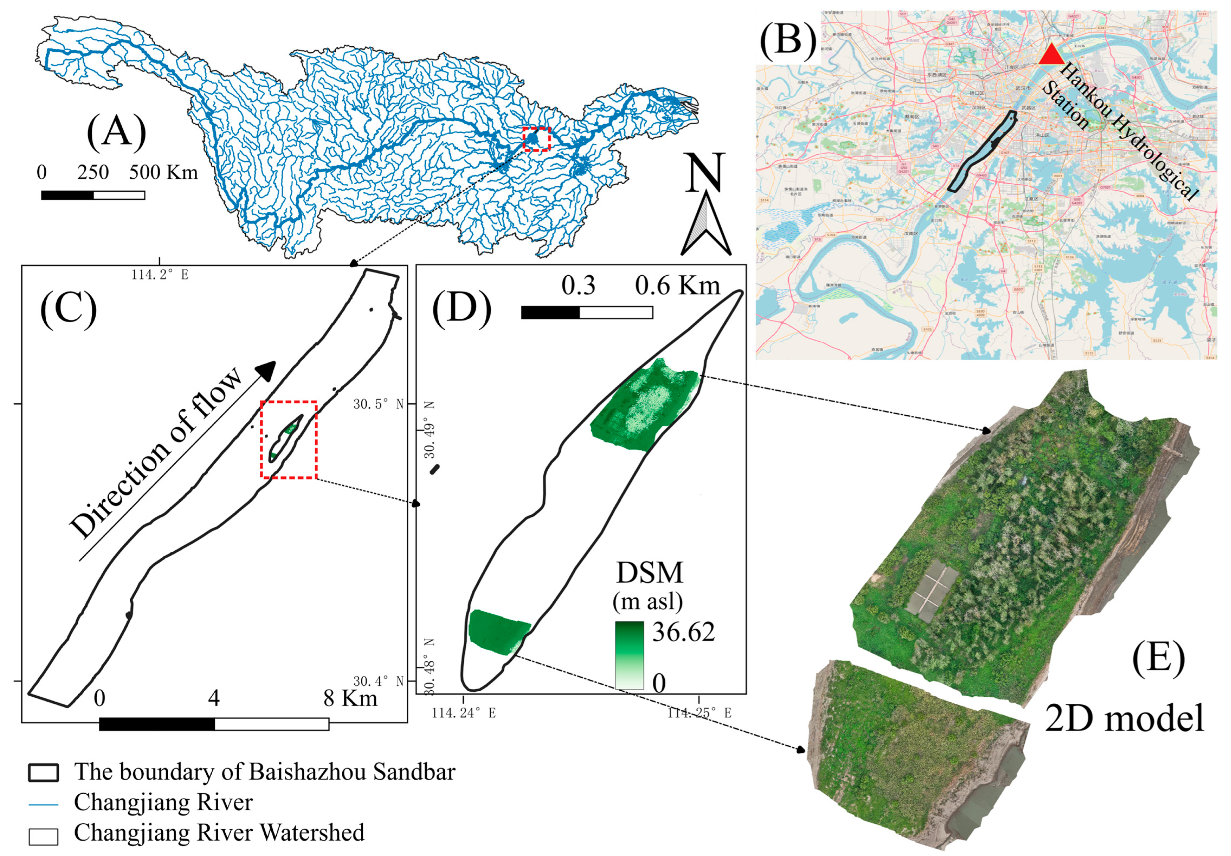
Figure 1. Location of the study area, (A,B) are the locations of the BSZ sandbar at the Changjiang River Basin and Wuhan city, respectively, (C) is the part of the river channel where the BSZ sandbar is located, (D) is the boundary of the BSZ sandbar and the Digital Surface Model (DSM) of the two mapped areas, (E) is the 2D model of the sampling areas.
Water 17 03160 g001
Figure 2. (A,B) are the flying paths of the left (A1) and right (A2) study areas, respectively. (C,D) are the aerial vehicle and the controller, respectively. Notably, the arrows in (A,B) indicate flight direction.
Water 17 03160 g002
Figure 3. Flow chart of the data processing, lately used to feed the FCNN model. Notably, solid blue arrows are used to connect the major steps in the framework, whereas hollow arrows are used to link the sub-steps within each major step.
Water 17 03160 g003
Figure 4. Distribution of the estimated vegetation height. (A) is the vegetation height of A2 and (B) is the vegetation height of A1.
Water 17 03160 g004
Figure 5. Distribution of (A) NDVI and (B) GNDVI in the flying areas.
Water 17 03160 g005
Figure 6. Comparison of linear and polynomial (degree = 2) regression models for vegetation height estimation. (A) Linear regression results and (B) polynomial regression training results. Notably, the red dashed line is the y = x line.
Water 17 03160 g006
Figure 7. Comparison of the vegetation height predicted by the trained FCNN model (y-axis) and real vegetation height (x-axis). Notably, the red dashed line is the y = x line.
Water 17 03160 g007
Table 1. Vegetation coverage of the two study areas.
Height (m)Coverage Area 1 (%)Coverage Area 2 (%)Whole Area A1 + A2 (%)
<295.3581.9885.36
2–42.134.443.86
4–61.123.112.61
6–81.032.452.09
>80.378.026.08
Disclaimer/Publisher’s Note: The statements, opinions and data contained in all publications are solely those of the individual author(s) and contributor(s) and not of MDPI and/or the editor(s). MDPI and/or the editor(s) disclaim responsibility for any injury to people or property resulting from any ideas, methods, instructions or products referred to in the content.