Article

GRU-Based Reservoir Operation with Data Integration for Real-Time Flood Control

1
Center for Built Environment (CBE), Sungkyunkwan University, Suwon 16419, Republic of Korea
2
Graduate School of Water Resources, Sungkyunkwan University, Suwon 16419, Republic of Korea
*
Author to whom correspondence should be addressed.
Water 2025, 17(21), 3039; https://doi.org/10.3390/w17213039
Submission received: 6 September 2025 / Revised: 9 October 2025 / Accepted: 20 October 2025 / Published: 22 October 2025
(This article belongs to the Special Issue Machine Learning Applications in the Water Domain)

Abstract

Reservoir operation serves as a critical non-structural measure for real-time flood management, aimed to minimize downstream flood damage while ensuring dam safety. This study develops and evaluates a Gated Recurrent Unit (GRU)-based reservoir operation model with data integration (DI) to enhance flood management capabilities. Optimal reservoir outflows are first determined for historical flood events using the Interior Point Optimizer (IPOPT), a deterministic optimization model designed to minimize peak outflows. The optimized hydrographs are compared with observed outflows to assess the benefits of improved operational strategies. GRU models are then trained and validated using inflow hydrographs and resulting optimal reservoir storage and release data. Various input configurations are tested, incorporating DI of lagged observations and forecasted values to evaluate their influence on model accuracy. The study also examines multiple hyperparameter settings to identify the optimal configuration. The methodology is applied to the Namgang Dam in South Korea, simulating hourly operations during flood events. Results indicate that historical reservoir inflow and storage are the most influential inputs, while adding precipitation (historical or forecasted) and/or forecasted inflows does not improve model performance. The GRU model with DI successfully replicates optimized reservoir operations, demonstrating its reliability and efficiency in flood management. This framework supports timely and informed decision-making and offers a promising approach for enhancing flood risk mitigation through improved reservoir operations.

1. Introduction

In South Korea, approximately 70% of annual precipitation occurs during the monsoon season from June to September [1]. As a key hydraulic infrastructure for water resources management, reservoirs have played a vital role in balancing water availability with growing socioeconomic demands [2]. To date, 22 multipurpose dams have been constructed across the country [3], serving the combined purposes of water supply, flood control, and hydropower generation [1]. These reservoirs are especially crucial in the context of increasing extreme weather events and flood risks.
Reservoir operation refers to the controlled release of water through dam spillway gates to manage storage levels and downstream flows [4]. During flood events, timely and appropriate reservoir operations can significantly mitigate disaster impacts [5,6]. Real-time reservoir operation rules define how much water to store or release at each time step, based on dynamic hydrological and meteorological conditions [7]. The dual goals of flood-oriented reservoir operation are to ensure dam safety and minimize flood risks upstream and downstream. However, this is a highly complex task, involving numerous constraints, uncertainties, and urgent decision-making requirements [8,9]. Operators must act quickly—often within hours—while facing limited data and poor predictability of evolving flood conditions.
Traditional reservoir operation models are generally categorized into two types. The first type is optimization-based models. These models aim to maximize benefits or minimize risks, such as flood damage, by identifying optimal operation strategies under defined objective functions [9,10]. Optimization often involves nonlinear objective functions with multiple constraints, making conventional methods such as Linear Programming (LP) or Dynamic Programming (DP) less effective or computationally burdensome [11]. While these models are well-suited for evaluating historical or idealized scenarios, they are less practical for real-time operation due to their high computational demands and difficulty in adapting to rapidly changing flood conditions [12]. The second type is simulation-based models. These include conceptual or physically based models that replicate reservoir behavior with lower computational requirements, making them more feasible for real-time application [13,14]. Advanced models such as WEAP [15] and HEC-ResSim [16] have been widely adopted, supported by advances in river dynamics modeling and computational capacity. These models combine empirical rule curves with mathematical formulations to simulate reservoir outflows and storage dynamics [17]. Their transparency and interpretability make them accessible to reservoir operators and facilitate informed water management [18]. However, physical-based models depend heavily on predefined rule curves and static operation policies, which may be inadequate under unexpected or extreme conditions, such as flash floods [19]. These models also do not incorporate the intuition and experience of operators—often essential during emergencies—and require detailed physical, hydrologic, and hydraulic parameters, which may not be available or accurate in real time. As such, their applicability to real-time reservoir operation is limited [17].
Machine learning (ML) has emerged as a powerful tool for simulating reservoir operations, offering the ability to efficiently learn complex operational rules from historical hydrological and reservoir datasets [20,21]. Unlike traditional models that rely on explicit mathematical formulations, ML models derive data-driven relationships between input variables (e.g., reservoir storage and inflow) and output variables (e.g., reservoir outflows), enabling flexible modeling without requiring full knowledge of physical processes [22]. Although ML methods are often considered “black boxes” due to limited interpretability, they excel at capturing nonlinear, high-dimensional, and dynamic relationships in water system [23], making them particularly suitable for real-time reservoir operation and outflow simulation.
Over the past decade, a variety of ML algorithms have been successfully applied to reservoir operation tasks, including Support Vector Machines (SVMs) [24], K-Nearest Neighbors (KNN) [25], Classification Regression Trees (CARTs) [26], Random Forests (RFs) [27], Multi-Layer Perceptrons (MLPs) [28], and Recurrent Neural Networks (RNNs) [2]. Among these, RNN-based models—including Long Short-Term Memory (LSTM) and Gated Recurrent Unit (GRU)—are particularly well-suited to sequential decision-making problems due to their ability to preserve both short- and long-term dependencies in time series data [2]. Wannasin et al. [29] compared RNN, LSTM, and GRU for reservoir simulation and concluded that GRU provided the most robust and accurate results, suggesting it as a promising option for practical applications in real-time water management.
In the context of deep learning-based forecasting, two main approaches are commonly used to incorporate recent observations: (1) data integration (DI), where lagged observations are explicitly included as input variables [30], and (2) variational data assimilation, where model states are adjusted in real-time to minimize errors between observations and simulations [31]. While data assimilation can be computationally intensive and complex to implement [31], DI offers a simpler and often more effective alternative [32]. In contrast to most LSTM/GRU models that rely solely on input sequences defined by time windows, where past data is processed implicitly, DI enables the model to explicitly learn short-term hydrologic patterns, improving accuracy and responsiveness [30].
Recent studies have demonstrated the effectivity of DI in enhancing deep learning models. Feng et al. [30] showed that incorporating lagged streamflow observations in LSTM inputs significantly improved hydrological forecasts. Song et al. [32] applied DI to improve snow water equivalent prediction using LSTM, showing its value for water resources management. However, to the best of our knowledge, DI has not yet been applied in deep learning-based reservoir operation models. This study addresses that gap by testing whether a GRU model with DI—explicitly accepting lagged observations as input—can outperform a standard GRU without DI in reservoir operation simulation.
To achieve this, we combine an optimization model with a machine learning model employing data integration, with three main objectives: (1) develop an optimization model to minimize peak reservoir outflows; (2) develop a machine learning model for real-time operation, trained on optimal hourly releases derived from the optimization model; and (3) assess the impact of different input variable sets, with and without DI, on the accuracy of the reservoir operation simulation.
This methodology is applied to the Namgang Dam in South Korea, which is particularly vulnerable to flooding due to its small storage capacity relative to its catchment area. According to the Korea Meteorological Administration, the southern region—including the Namgang watershed—is experiencing increasing rainfall intensity, elevating flood risks. Despite this, the Namgang Dam remains the only multipurpose dam in the country without completed response measure for extreme floods [33]. In this study, an optimization model is first used to derive optimal reservoir operating rules for flood control at Namgamg Dam. The optimized outflow hydrographs are then compared to historical operations to evaluate the improvement. Next, a GRU model is trained on reservoir inflow, and storage and release data generated by the optimization process. The study also explores various scenarios to evaluate the effects of input variable selection, the inclusion of lagged observation via DI, and the impact of forecasted inputs on model performance.

2. Site and Materials

The Namgang Dam is located on the Nam River (35°15′ N, 128°23′ E), a tributary of the Nakdong River, and serves multiple purposes including flood control and water supply [34]. The dam creates the Jinyang Reservoir, which has a catchment area of 2285 km2 and a total storage capacity of 309.2 million m3. The reservoir covers a surface area of 28.2 km2 [3]. The primary inflows originate from the Kyeongho and Duckcheon Rivers (Figure 1), with the Kyeongho River contributing runoff from a 1773.2 km2 watershed—approximately five times the size of the Duckcheon River basin, which drains an area of 354.6 km2 [34]. The design flood level of the Namgang Dam is 46 EL.m, while both the normal high-water level and the flood season restricted water level are set at 41 EL.m. The minimum operating level is 32 EL.m [3].
This study employs hourly data on reservoir inflow, storage, release, and precipitation obtained from the My Water platform (www.water.or.kr, accessed on 21 February 2025), spanning a 25-year period from 2000 to 2024. The analysis focuses on reservoir operations during flood events. A total of 42 significant flood events—each with peak reservoir inflows exceeding 3000 m3/s—were identified and are summarized in Table 1. The historical maximum peak inflow recorded at the reservoir is 14,818.0 m3/s. All peak flow events occurred between June and September, aligning with the region’s primary rainy season influenced by the East Asian monsoon, tropical cyclones, and convective storms [35]. This storm-based approach offers practical insights into the planning and design of flood management infrastructure to better protect downstream communities and ecosystems [36,37].

3. Methodology

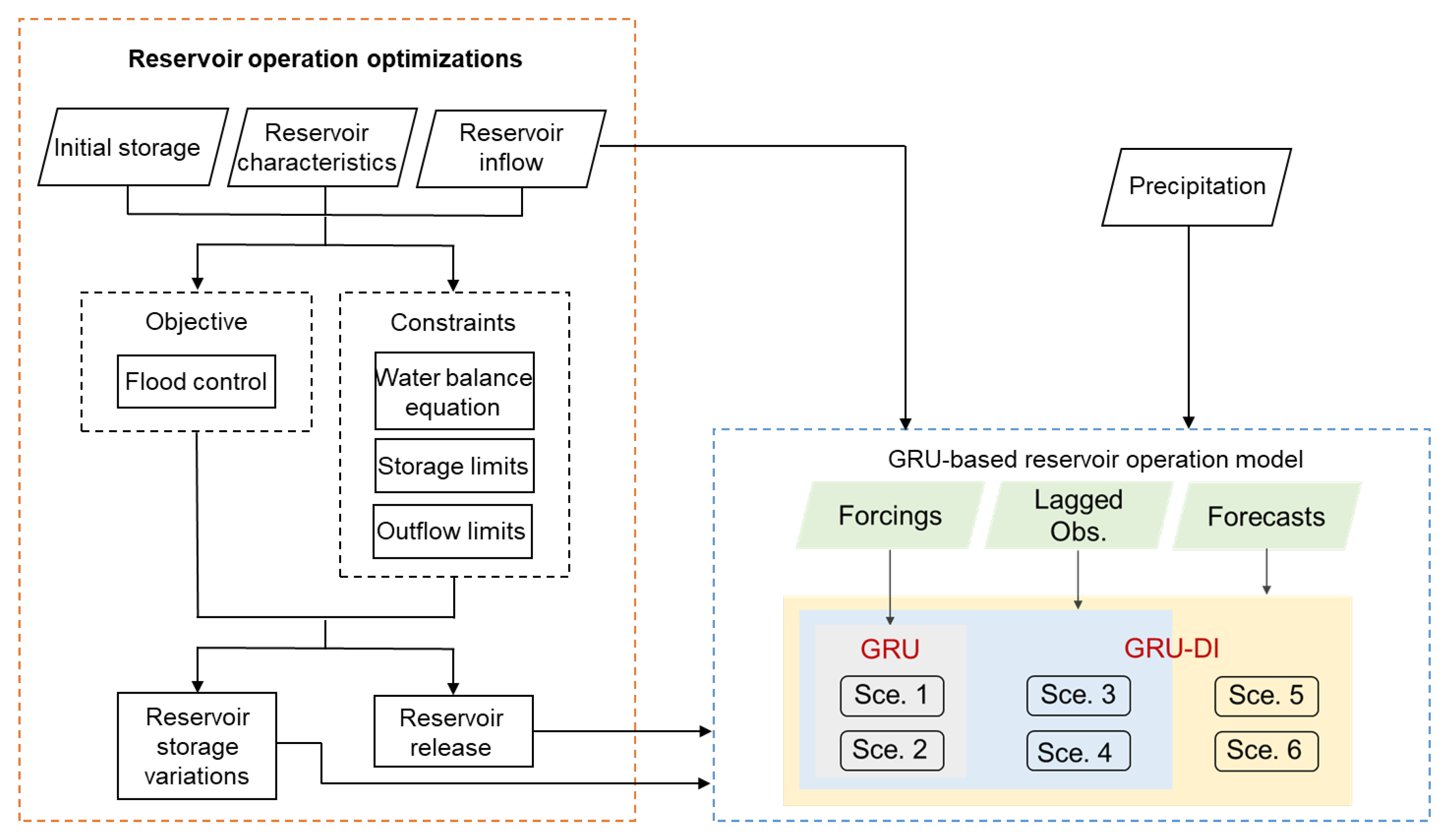
This study proposes an integrated methodology that combines a reservoir operation optimization model with a data-driven machine learning model to improve flood control performance. Figure 2 illustrates the workflow of the proposed approach, which aims to minimize downstream flood damage while ensuring dam safety. The optimization model is first used to derive optimal reservoir release rules for a range of historical flood events. The resulting optimal release and storage data, along with the corresponding inflow hydrographs, are then used to train, validate, and test a machine learning-based real-time reservoir operation model.

3.1. Reservoir Operation Optimization Model

The objective of the reservoir operation optimization is to minimize the downstream flood damage by reducing the peak flow of reservoir release hydrographs. The optimization model determines reservoir outflow hydrographs based on given inflow patterns and initial storage conditions. The objective function Z is defined as follows:
Minimize Z = maxt=1,…,T Rt
in which Rt is the reservoir outflow at time t, and T is the flood duration.
Constraints of the model are as follows:
S t = S t t + I t t t R t t t           t = 1 ,   ,   T
0 S t S m a x
0 R t R t m a x ( S t )           t = 1 ,   ,   T
in which S t is the reservoir storage at time t, I t t is the inflow to the reservoir at time t t , and t is taken as 1 h in this study. S m a x is the maximum reservoir storage, and R t m a x ( S t ) is the maximum outflow capacity of the reservoir based on the reservoir volume and volume–outflow curve.
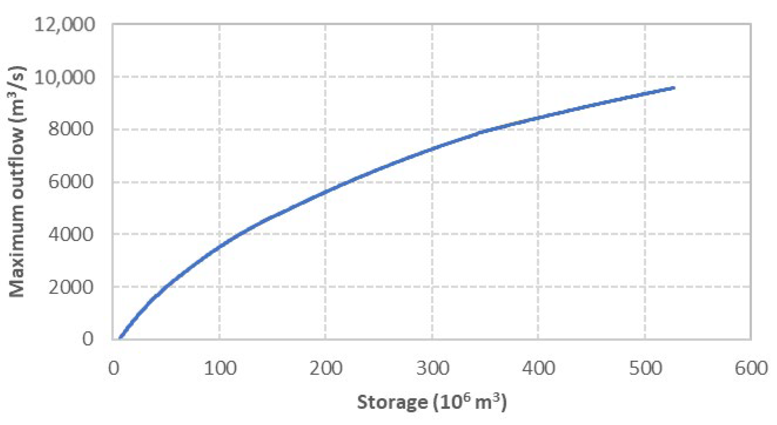
To constrain reservoir outflows, a volume–outflow relationship is established based on the water level-storage relationships for different sections of reservoir, coupled with the combined discharge capacities of all outlet structures (Figure 3). This relationship defines the maximum allowable outflow corresponding to the reservoir’s storage volume. It is incorporated into the optimization model as a constraint (Equation (4)). During the optimization process, reservoir storage is updated at each time, and the corresponding maximum outflow is applied to ensure feasible and physically realistic solutions.
This study employs the Interior Point Optimizer (IPOPT) to solve the reservoir flood operation optimization problem. Reservoir flood control represents a large-scale, nonlinear, and constrained optimization challenge. IPOPT is an open-source solver [38] specifically developed to address such problems efficiently. It uses a primal-dual interior-point algorithm combined with a filter line-search strategy [39]. Inequality constraints are handled through the use of logarithmic barrier functions, introducing a barrier parameter that transforms the original problem into a sequence of equality-constrained sub-problems. As the barrier parameter is progressively reduced, these sub-problems are solved iteratively [40]. For each iteration, IPOPT applies a Newton-type algorithm with a line search that involves solving large, sparse, symmetric, and potentially indefinite linear systems. This approach ensures robust convergence and high computational performance, particularly in large-scale dynamic optimization tasks [41]. In this study, the optimization framework is implemented in Pyomo 6.7.3 [42], a Python-based algebraic modeling language that facilitates clear and intuitive representation of mathematical models. Pyomo serves as the interface for defining the optimization problem and transferring it to IPOPT for solution.

3.2. GRU-Based Reservoir Operation Model

The Gated Recurrent Unit (GRU), introduced by Cho et al. [43], is an advanced variant of the traditional Recurrent Neural Network (RNN). GRUs share structural similarities with Long Short-Term Memory (LSTM) networks, particularly in their use of gating mechanisms to regulate the flow of information. However, GRUs offer a more streamlined architecture by reducing the number of gates, thereby simplifying computations while maintaining comparable performance [44]. Several studies have shown that GRUs can deliver performance on par with LSTMs, but with improved training efficiency and faster execution [45]. For instance, Gao et al. [45] developed both LSTM- and GRU-based models for short-term runoff forecasting and found GRUs to be preferable due to their reduced training time and comparable predictive accuracy.
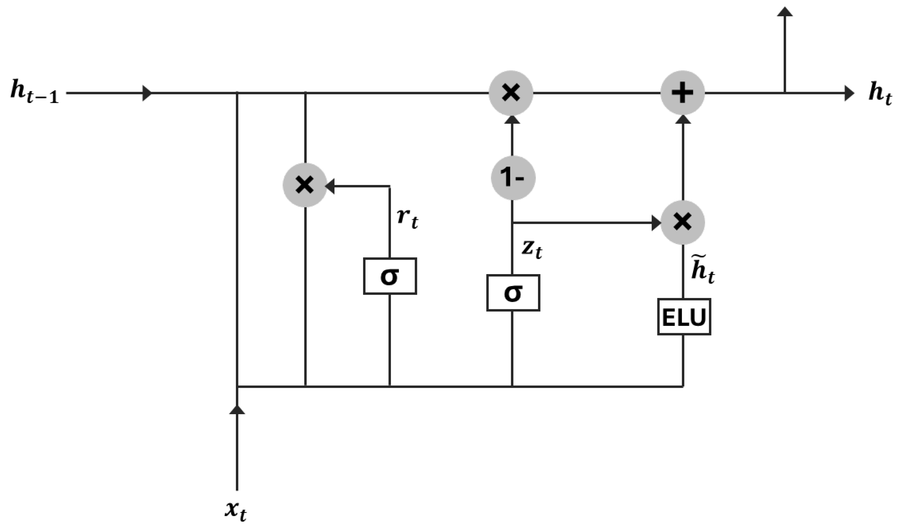
As illustrated in Figure 4, the GRU architecture enhances the memory capacity of standard RNNs while improving training stability and efficiency [44]. By employing gating mechanisms and hidden units, GRUs mitigate the vanishing gradient problem often encountered in traditional RNNs. Each GRU unit adaptively captures temporal dependencies across different time scales, making it well-suitable for sequential data modeling.
At each time step, the GRU processes two inputs: the current input x t and the previous hidden state h t 1 , which encapsulates information from prior time steps. The resulting output y t is derived from the hidden node, while the updated hidden state h t is forwarded to the next time step [46].
Unlike LSTM, which uses three gates (input, forget, and output), the GRU simplifies the architecture by using only two gates. One is the update gate (zt) that determines the extent to which past information should be retained in the current state. A higher value indicates greater retention. The other is the reset gate ( r t ) that controls the degree to which past information is forgotten. A lower value results in greater forgetting of previous state.
These gates enable GRUs to capture long-term dependencies while reducing model complexity and computational cost. The mathematical formation of the GRU is provided in Equations (5)–(9) [47,48]:
r t = σ w r · h t 1 , x t + b r
z t = σ w z · h t 1 , x t + b z
h ~ t = E L U w h ~ · r t h t 1 , x t
h t = 1 z t h t 1 + z t h ~ t
  y t = σ w o · h t
where σ denotes the sigmoid activation function, which bounds the output between 0 and 1. Additionally, the Exponential Linear Unit (ELU) activation function is employed to introduce nonlinearity, allowing for negative values and enhancing convergence speed by increasing neuron diversity and smoothing activation dynamics.
In this study, the GRU model is employed to simulate reservoir operations under flood conditions. The model is trained to estimate reservoir outflows using input features such as inflow hydrographs, precipitation data, and optimized reservoir storage and release values derived from a reservoir operation optimization model. The modeling is conducted at an hourly resolution during selected flood events.
To train the model, the dataset is divided into predictor variables (inputs) and a target variable (output). The primary predictor is reservoir inflow, which captures the upstream hydrological response. Precipitation is also included, as it directly influences inflow and storage dynamics. Another key input variable is the reservoir’s storage volume, a commonly used determinant of release decisions. Storage-based operational rules typically aim to satisfy multiple objectives, including water supply, flood control, irrigation, and hydropower generation [18]. The target variable is the hourly reservoir outflow at the current time step. With this structured input-output setup, the GRU-based reservoir operation model is developed to enhance real-time decision-making during flood events.

3.3. Scenarios

To evaluate the impact of different input combinations and application of DI, six scenarios are tested, as summarized in Table 2. The selection of input variables and their time lags is known to significantly influence the performance of machine/deep learning models [49,50]. Scenario 1 uses reservoir inflow and storage at time step t−1 as input variables. Scenario 2 adds precipitation at t−1 to examine its influence on GRU-based reservoir operation modeling. Scenarios 3 and 4 extend Scenarios 1 and 2, respectively, by integrating lagged observations over the past three hours into the GRU input, thereby incorporating DI. Scenarios 5 and 6 additionally include short-term forecasts (up to two days ahead) of inflow and precipitation, considering the importance of forecasting in operational decision-making [51,52]. Forecasts are assumed to be perfectly accurate and are generated from observed data.

4. Results and Discussion

Optimal reservoir storage and release trajectories for 42 historical flood events are generated using IPOPT, based on inflow hydrographs and initial storage conditions. These optimal values serve as training targets for GRU model development. The dataset is split into training (52%), validation (25%), and testing (23%) sets (Table 3).
In this study, hyperparameter tuning focuses on three key parameters: window size, number of hidden nodes, and batch size. Fixed hyperparameters include dropout rate (0.2), learning rate (0.001), number of hidden layers (1), loss function (MSE), optimizer (RMSprop), and activation function (ELU). The number of hidden nodes is tuned within the range of 1–100. Early stopping with a maximum of 10,000 epochs is applied, and the number of epochs is not considered as a tuning parameter. Hyperparameter configurations are summarized in Table 4.
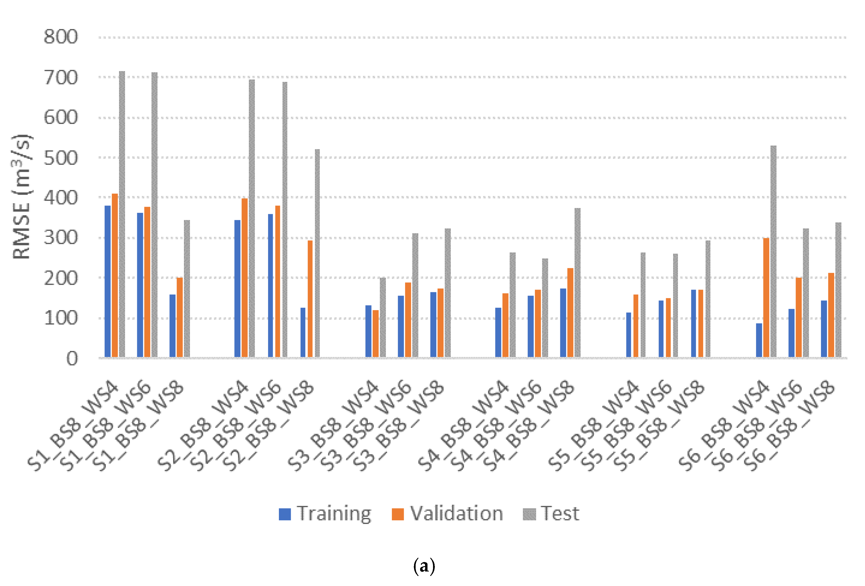
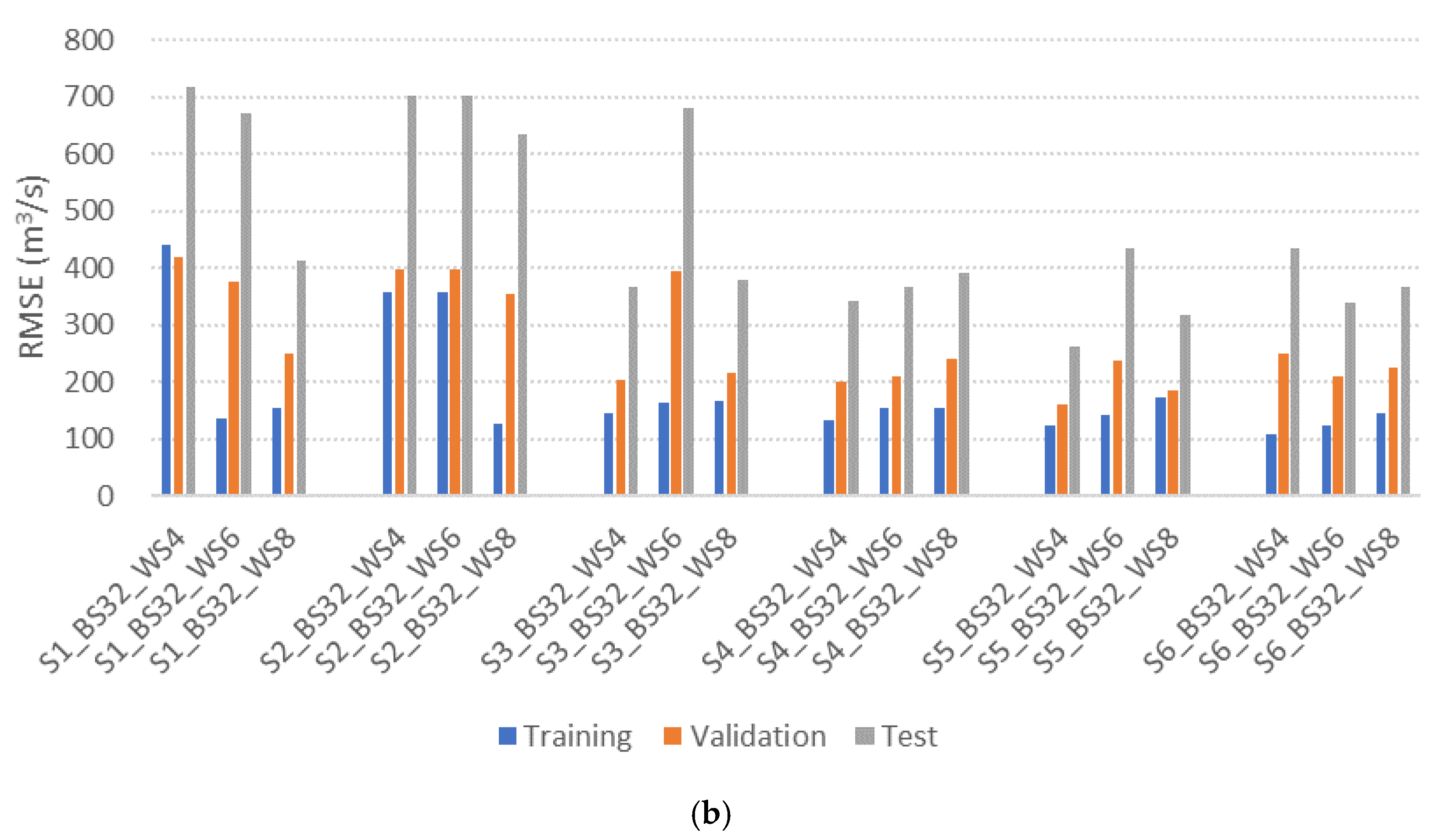
GRU model performance under different input scenarios and hyperparameter settings is presented in Table 5. To assess the impact of batch size and window size, Root Mean Squared Error (RMSE) and Nash-Sutcliffe Efficiency (NSE) values calculated using Equation (10) and Equation (11), respectively, are compared across multiple configurations. The number of hidden nodes is optimized in each setting using the RMSprop optimizer. Figure 5 shows the RMSE values using bar charts (e.g., S1_BS8_WS4 refers to Scenario 1 with batch size 8 and window size 4).
R M S E = 1 n i = 1 n Q o p t ,   i Q s i m ,   i 2
N S E = 1 i = 1 n Q o p t , i Q s i m ,   i 2 i = 1 n Q o p t , i Q ¯ o p t ,   i 2
where Q o p t ,   i is the ith optimized reservoir outflow, Q s i m , i is the ith GRU-simulated outflow, and n is the number of data points.
Models with DI (Scenarios 3 and 4) trained with a batch size of 8 consistently outperform those with a batch size of 32. This indicates that smaller batch sizes may offer improved learning stability and responsiveness in DI-based model, likely due to their ability to better capture high-frequency variability in short hydrological sequences. In scenarios without DI (scenarios 1 and 2), a window size of 8 yields the best performance. In contrast, DI-based models (Scenarios 3 and 4) achieve optimal performance with window sizes of 4 and 6, respectively. For DI-based models incorporating forecasted variables (Scenarios 5 and 6), a window size of 6 provides the highest accuracy. These results indicate that GRU models with DI can achieve superior performance using shorter window sizes compared to those without DI. This finding is consistent with previous work by [30], which showed that DI enables models to capture short-term hydrologic dynamics more effectively by explicitly providing lagged observations as input features.
The best model performance is observed in S3_BS8_WS4, with a minimum RMSE of 202.2, an NSE of 0.93, and a coefficient of determination (R2) of 0.89, followed by S4_BS8_WS6, which records a RMSE of 250.19, NSE of 0.90, and R2 of 0.90. GRU models incorporating DI (scenarios 3 and 4) consistently outperform those without DI (scenarios 1 and 2), emphasizing the importance of explicitly incorporating recent observations in model training. This feature is especially critical for real-time flood operation, where quick decision-making is essential. Interestingly, S3_BS8_WS4, which relies solely on past inflow and storage observations, outperforms S4_BS8_SW6, which includes past precipitation as an input. This suggests that adding past precipitation does not enhance model accuracy, potentially due to data redundancy, as inflow and storage already encapsulate much of the system’s hydrological behavior.
The inclusion of forecasted values in Scenarios 5 and 6 leads to improved accuracy in certain model configurations. However, the highest performance is achieved by the DI model utilizing only historical inflow and storage. These outcomes suggest that while forecasted data can provide additional information, its utility is limited and does not significantly enhance model accuracy. This may be due to the short lead times of forecasted inputs, which can compromise their reliability. Consequently, models based on recent historical data offer more robust and interpretable solutions, which are critical for real-time applications like reservoir operation.
Despite the satisfactory performance of the models, further improvements are possible. In this study, several hyperparameters were manually tuned or selected, and no systematic hyperparameter optimization was performed. Future studies could benefit from more systematic hyperparameter optimization methods to further improve model performance. Nevertheless, the objective of this study is not solely to minimize RMSE or maximize NSE, but rather to identify key input variables for reservoir outflow prediction and evaluate the impact of DI and forecasted forcing on GRU model performance. Thus, the findings provide insights into effective model design for reservoir outflow prediction under real-time constraints.
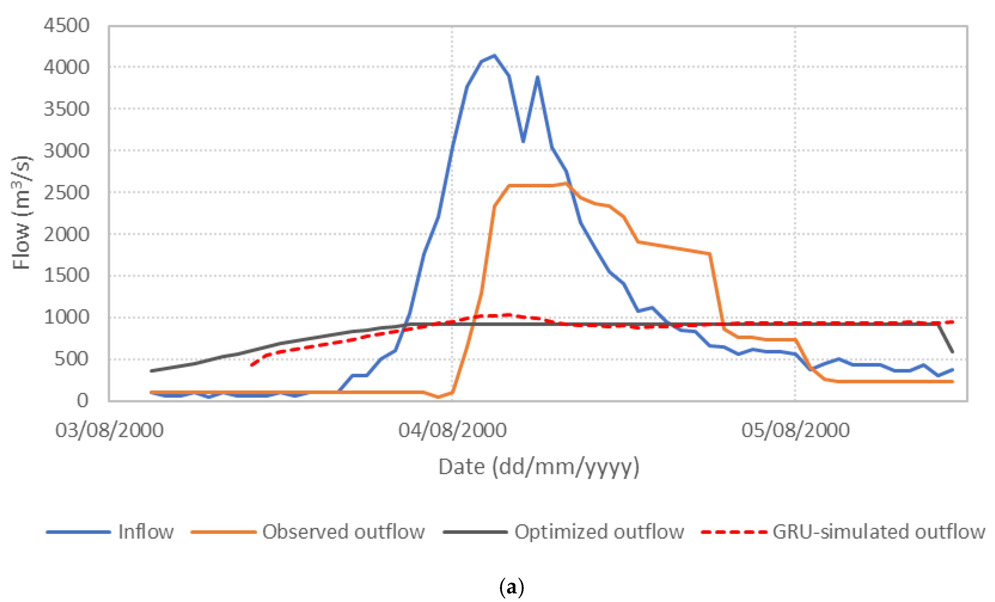
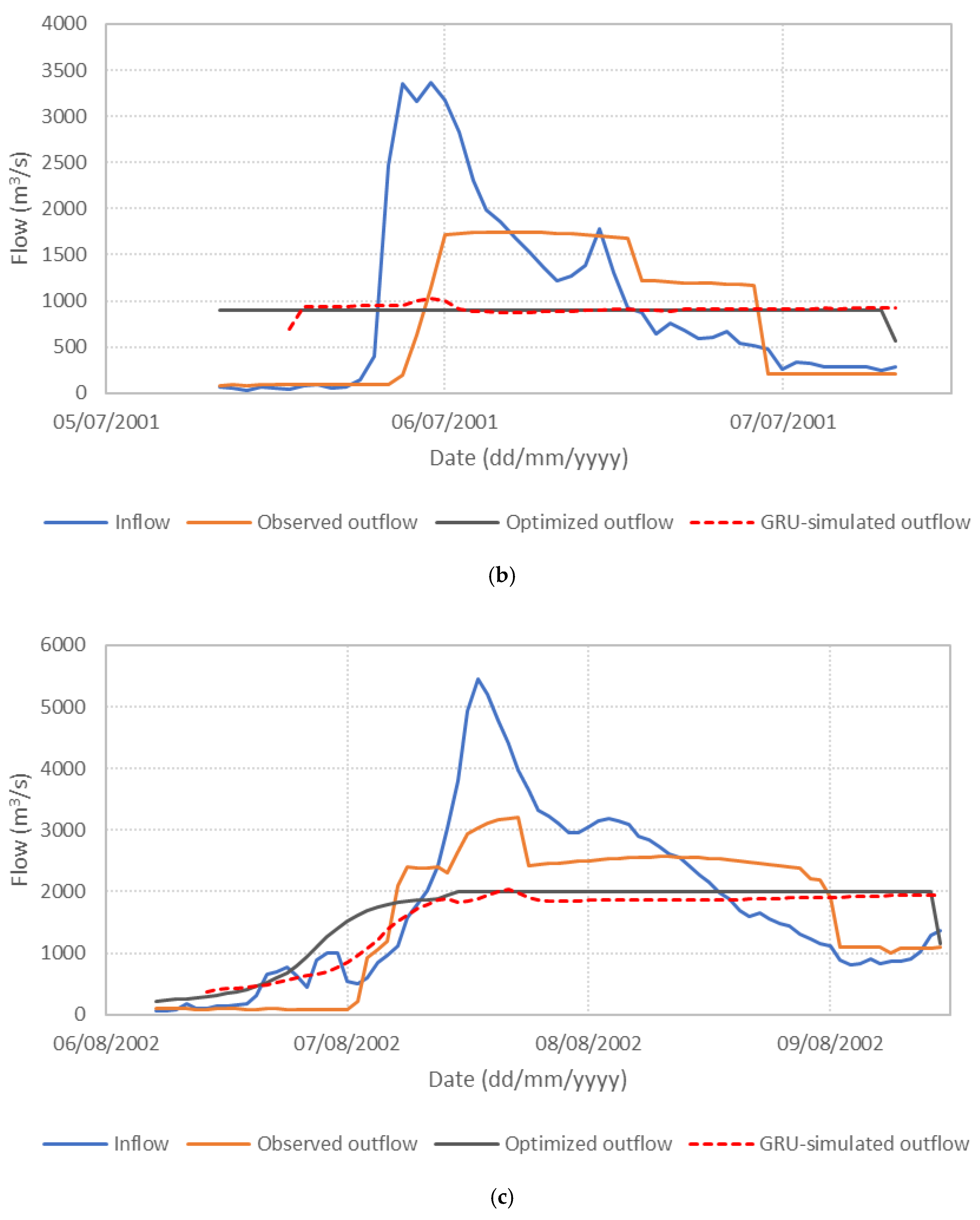
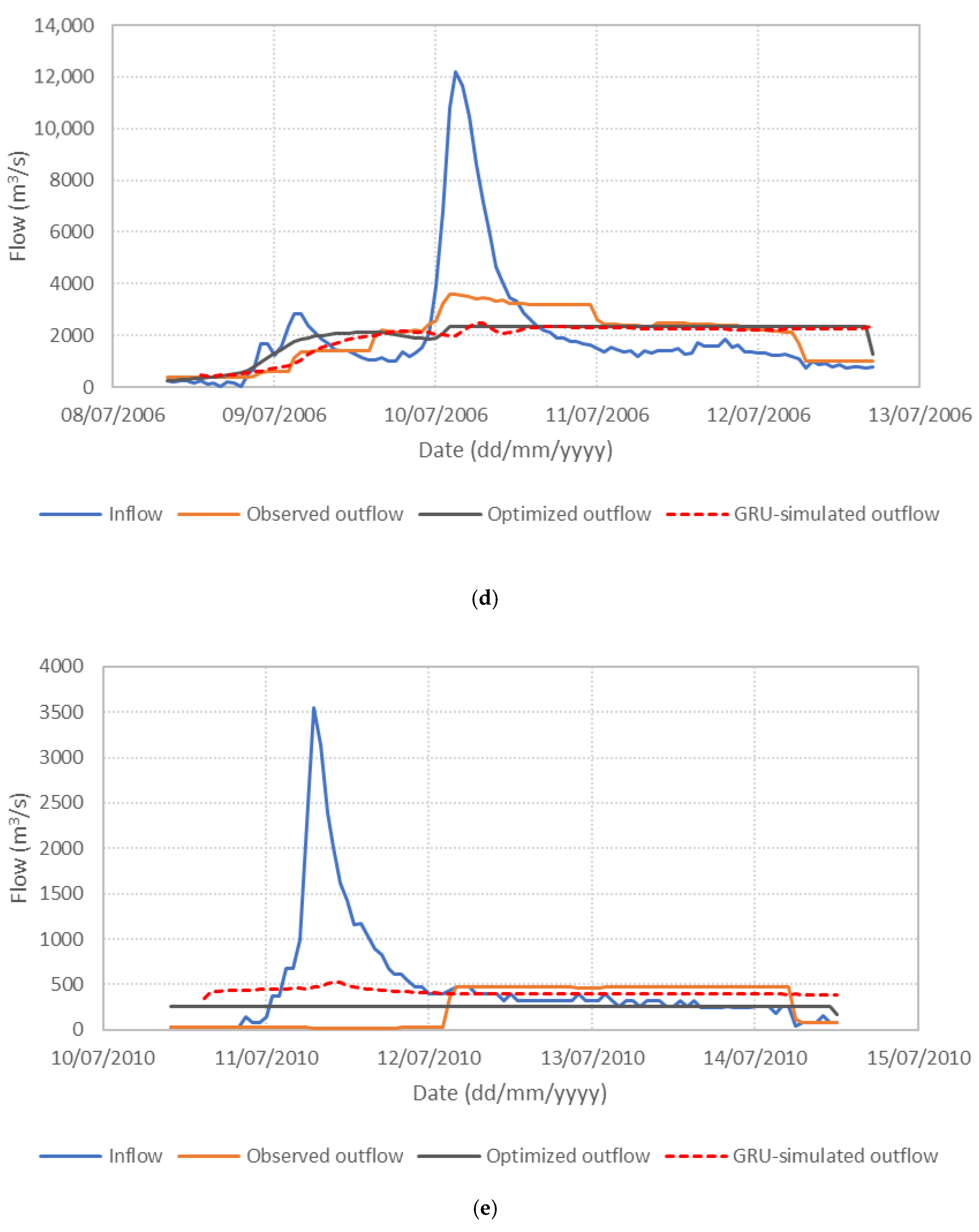
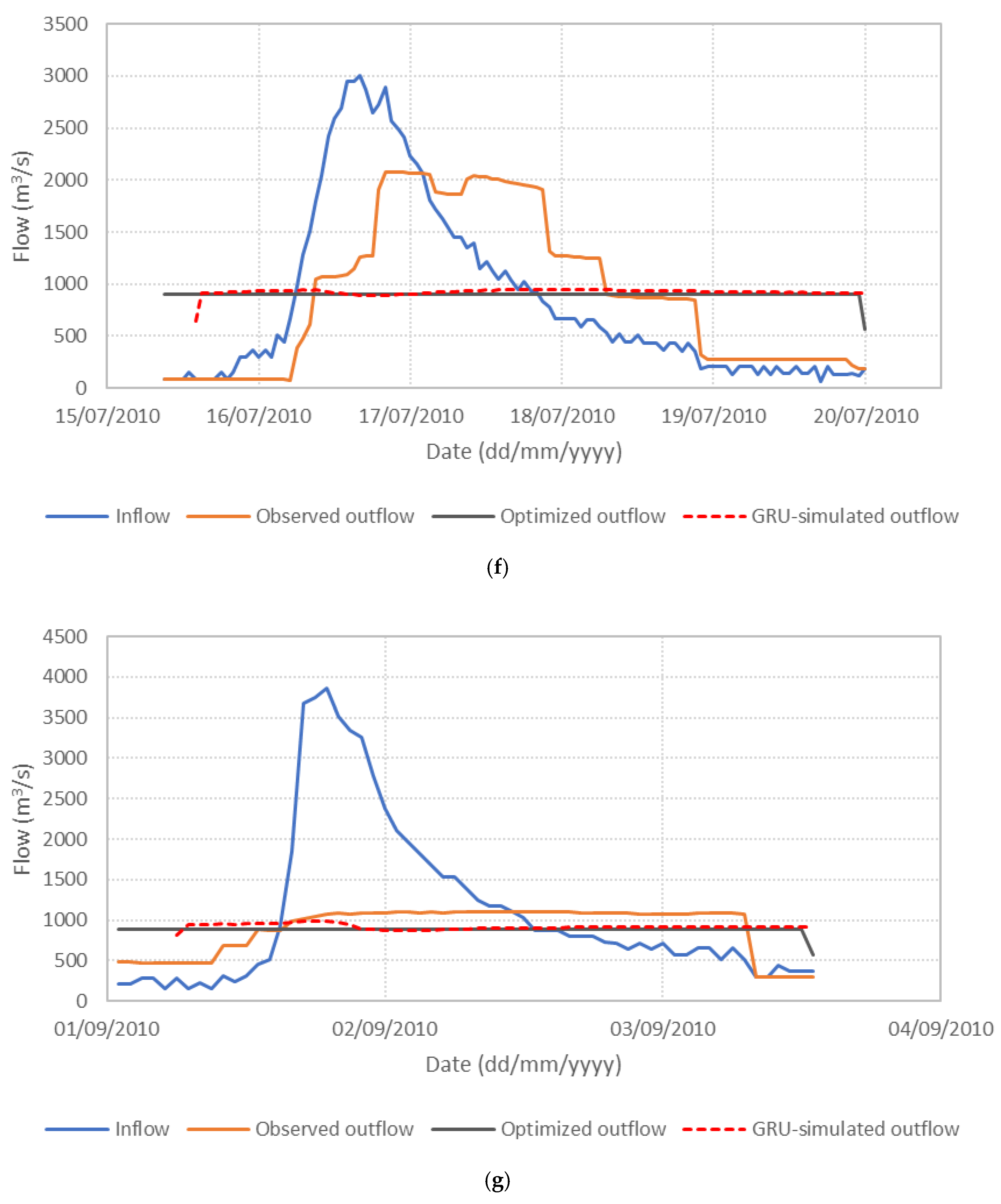
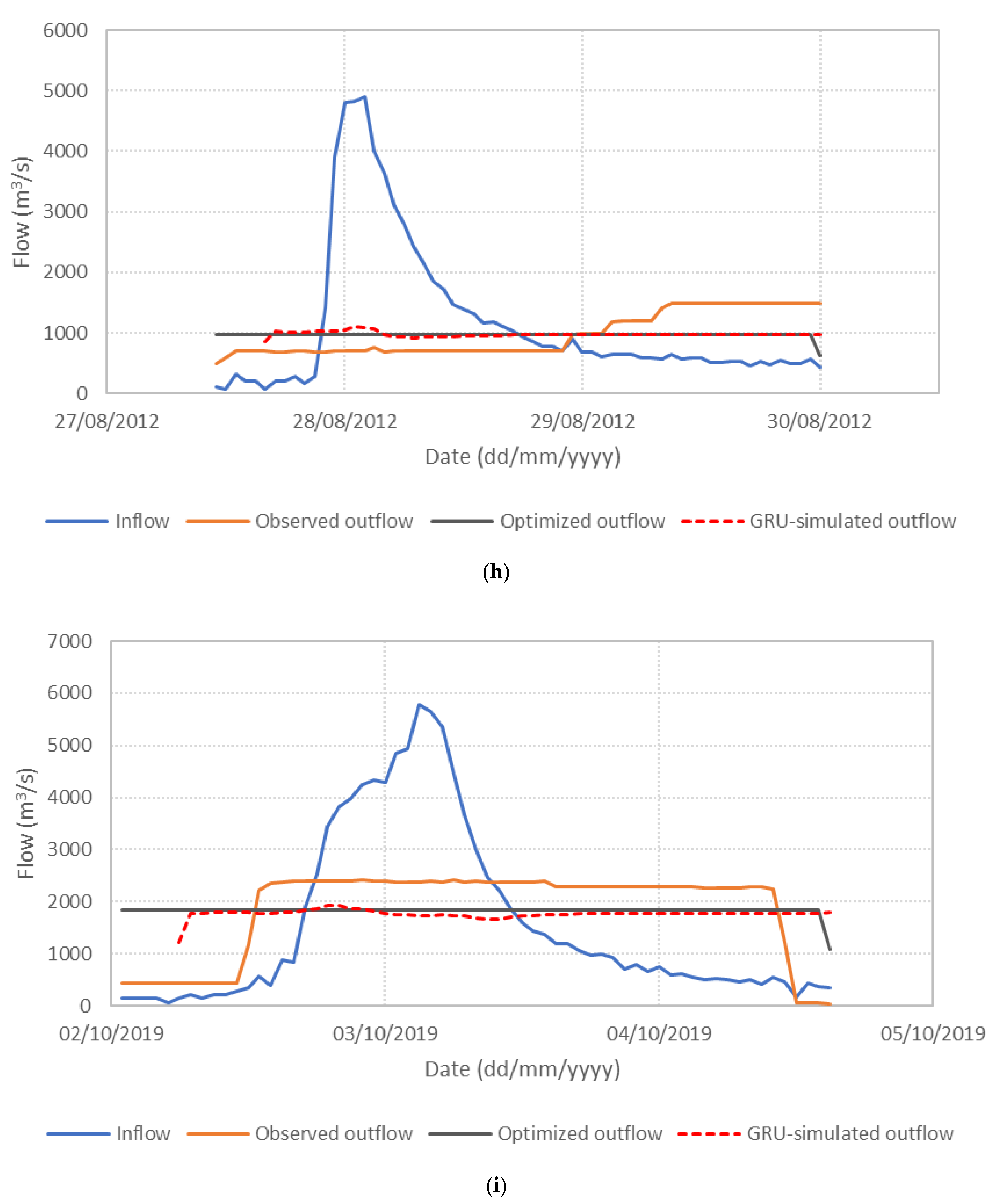
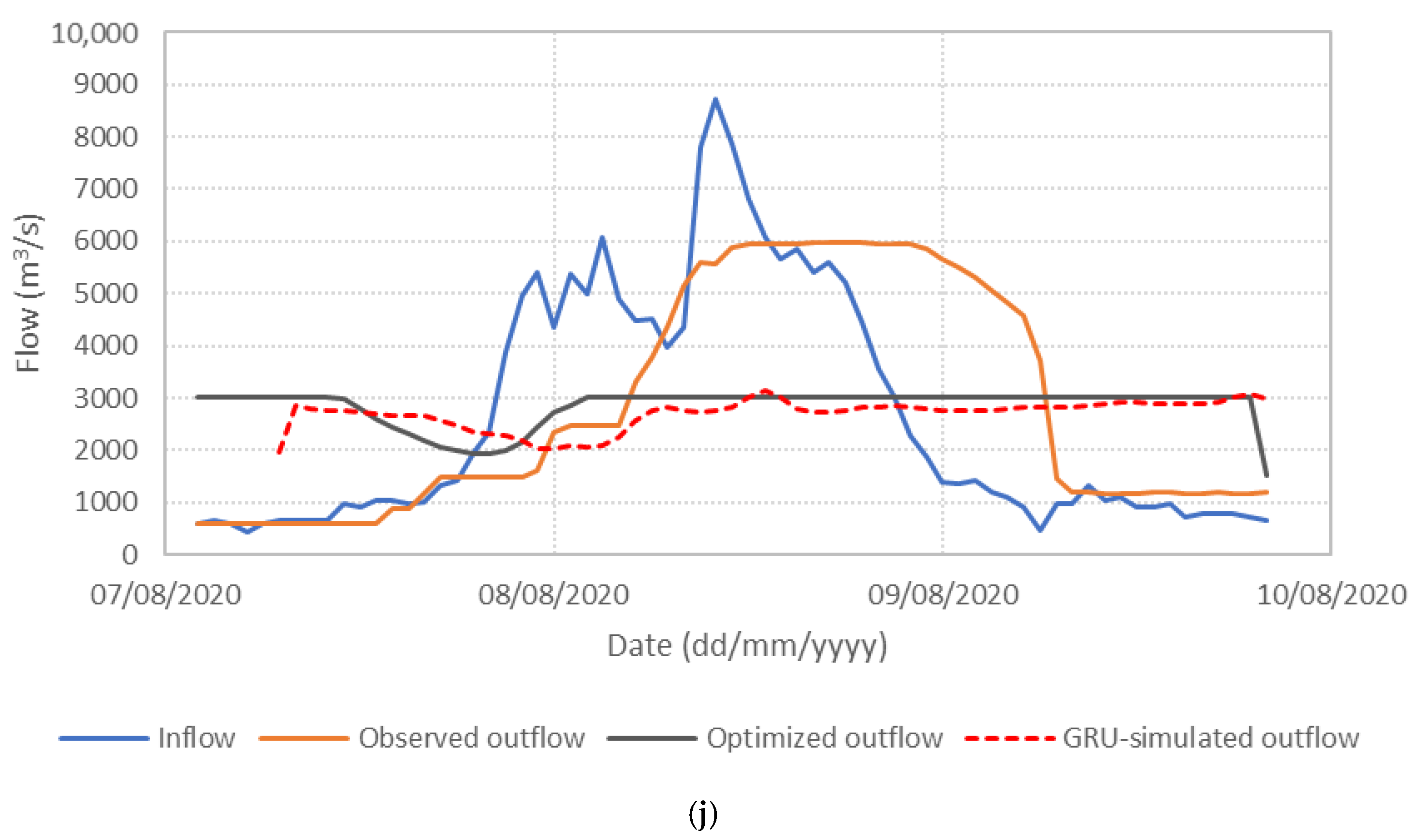
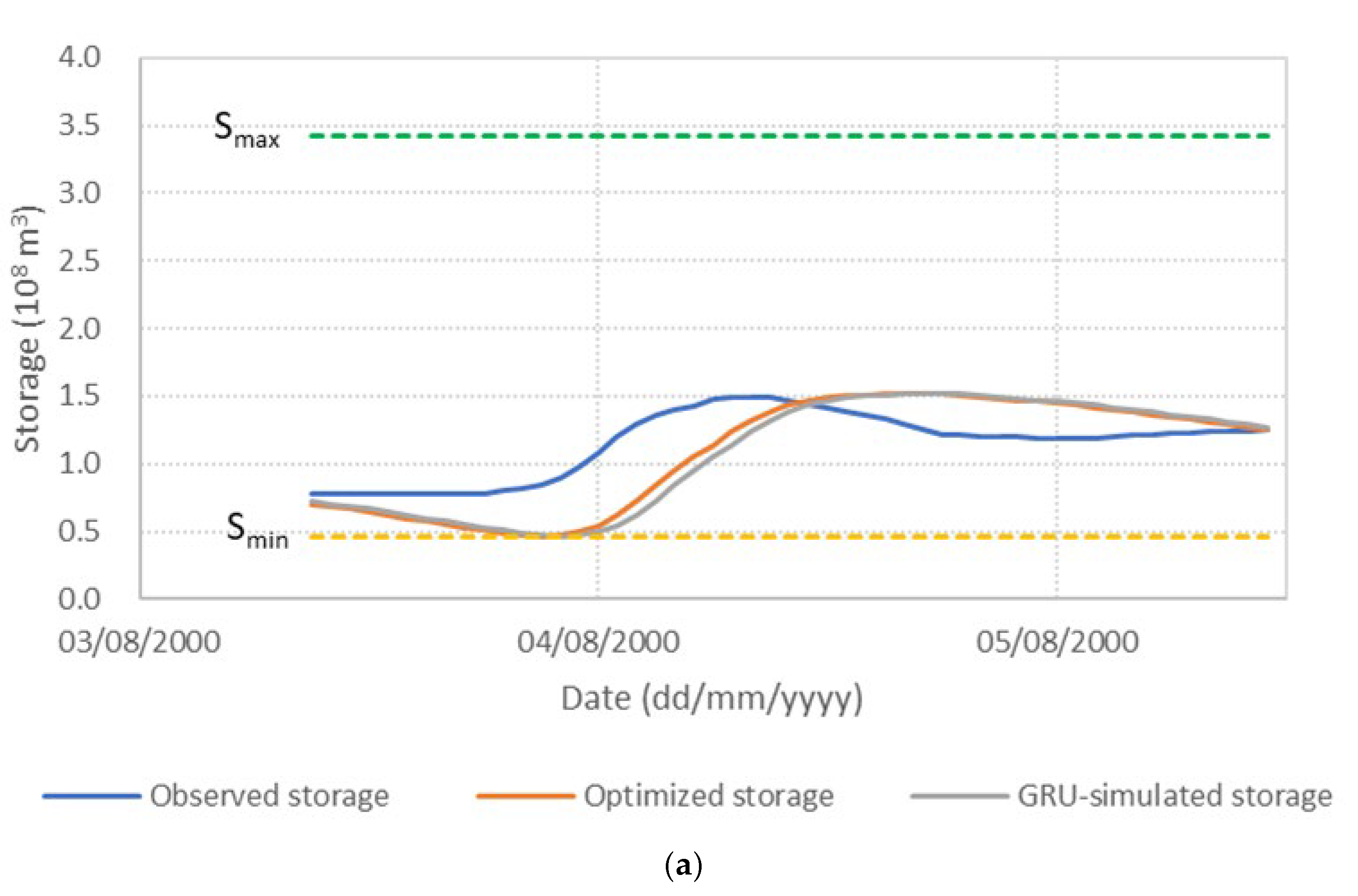
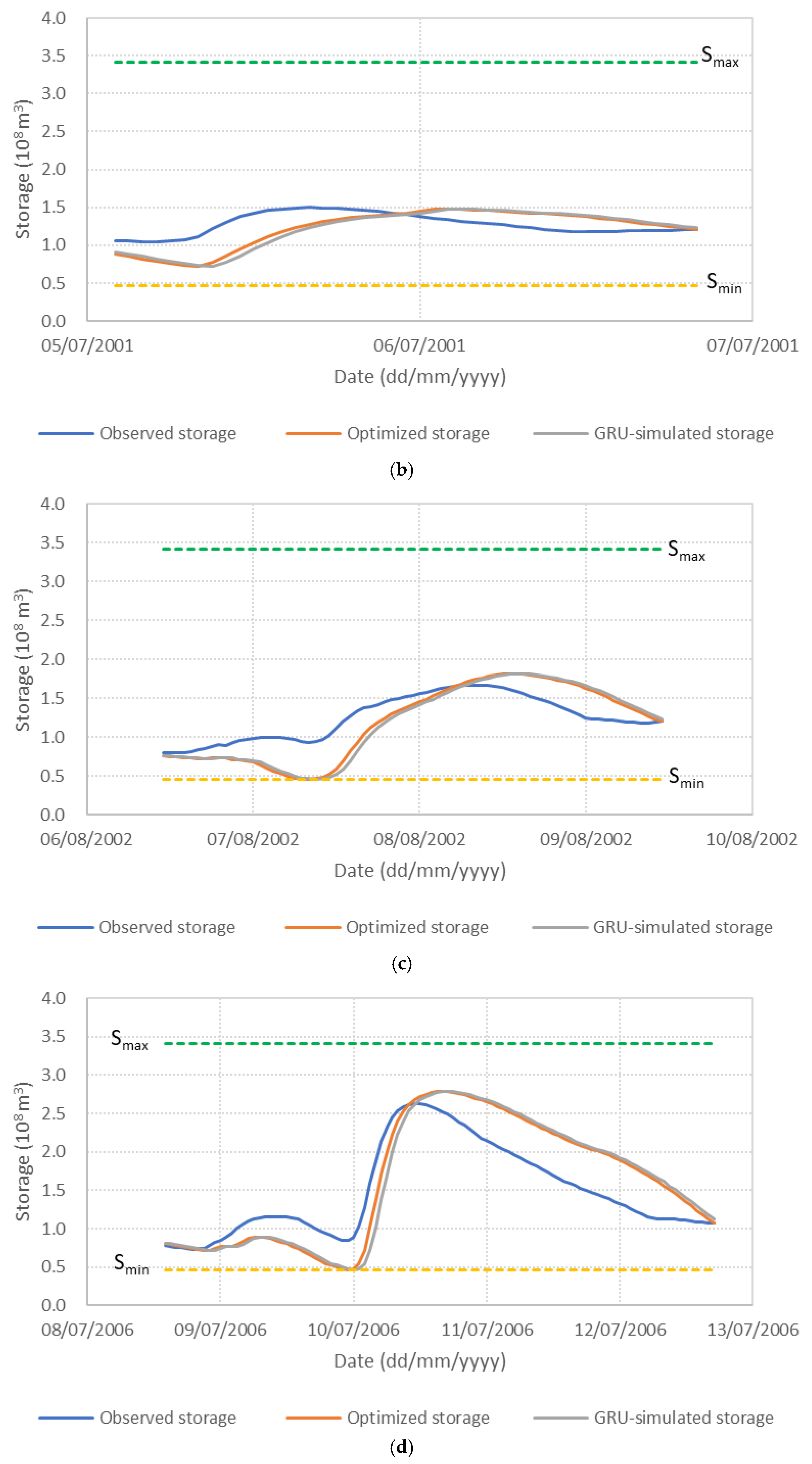
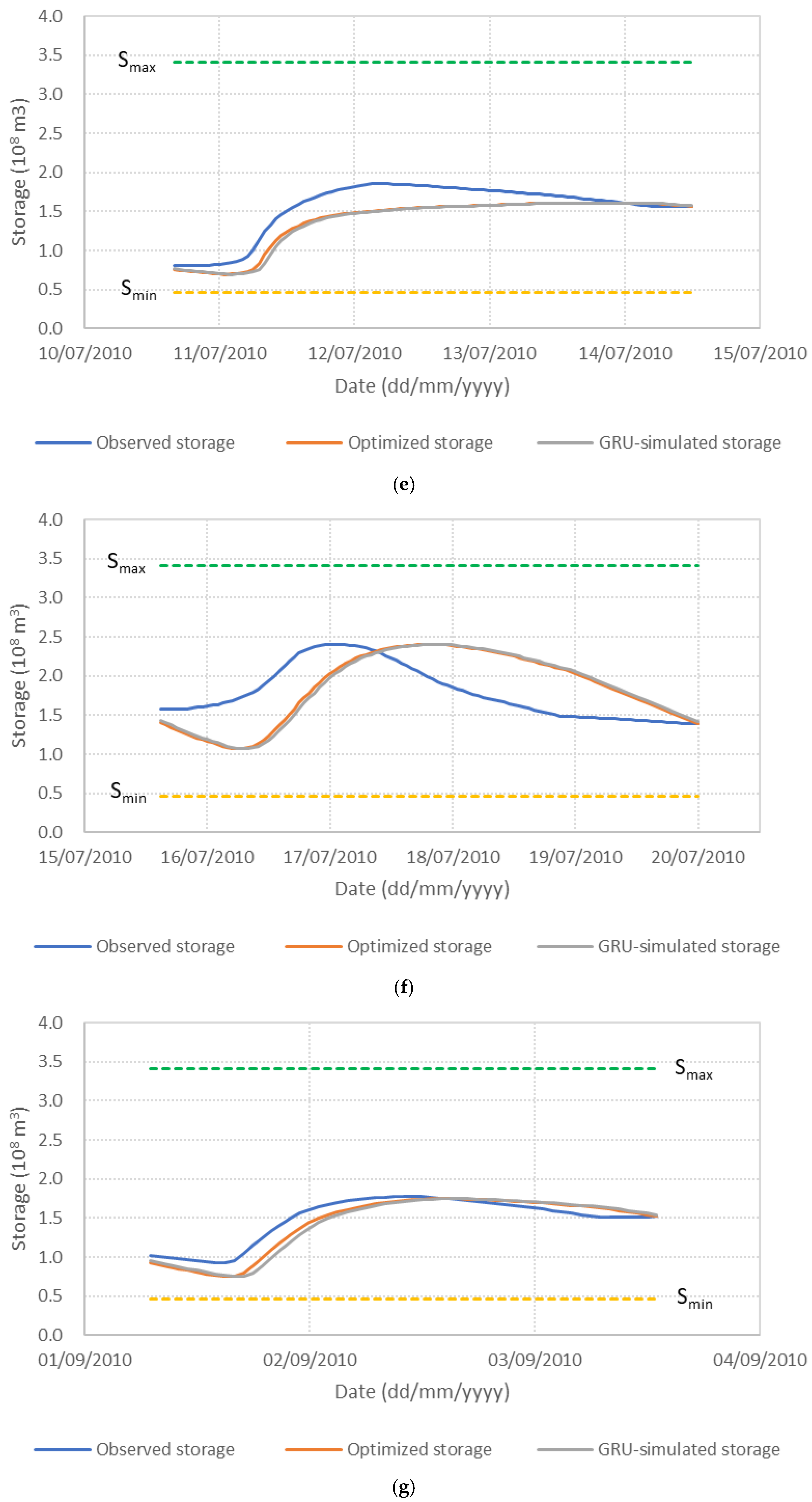
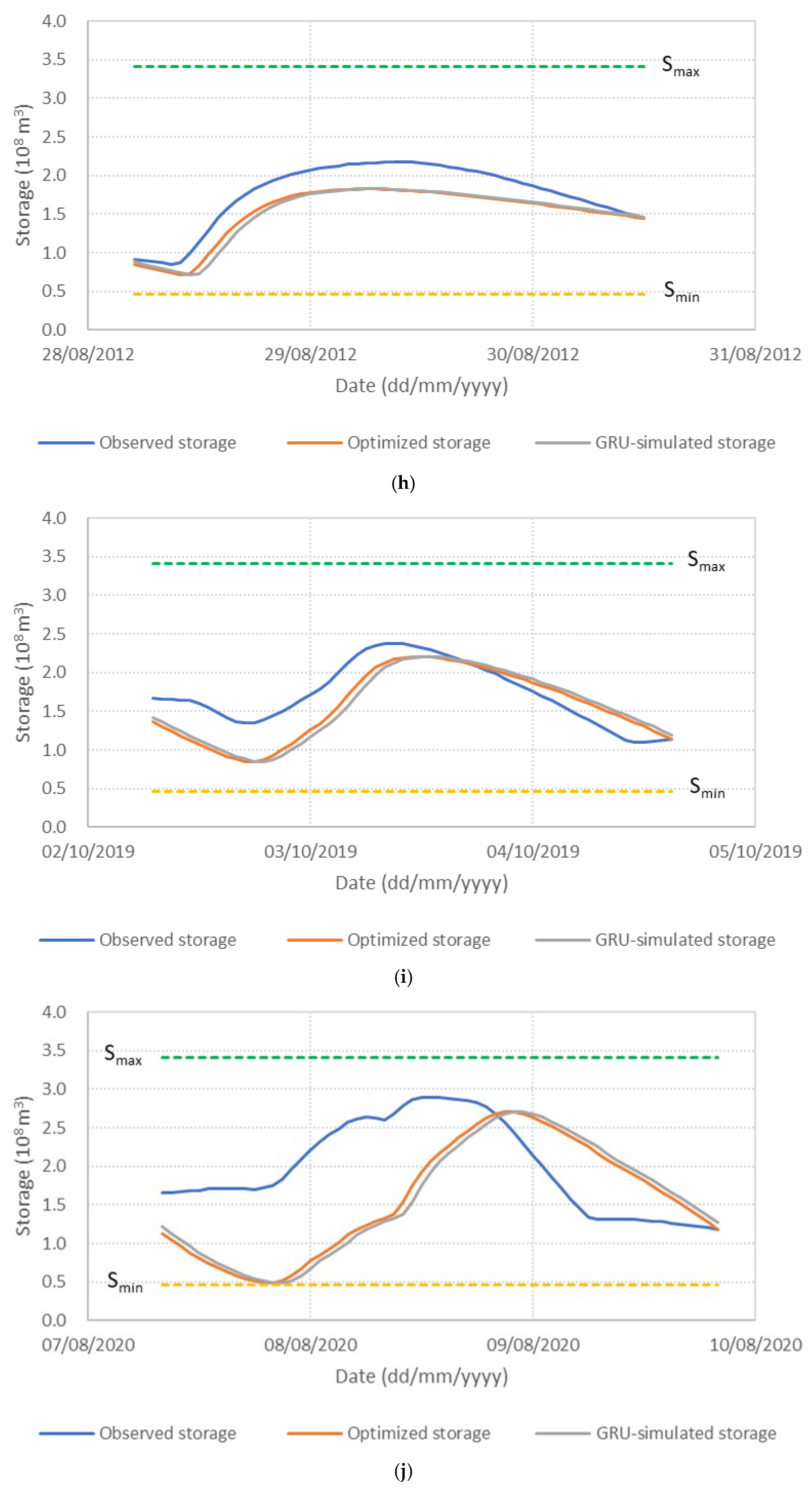
Figure 6 presents the performance of the S3_BS8_WS4 model, comparing observed, optimized, and GRU-simulated outflows during the test periods. The results show that the optimized release hydrographs consistently demonstrate reduced peak discharges compared to observed historical operation. This supports the premise outlined in the Introduction that optimization-based approaches can effectively mitigate downstream flood risk. The GRU-simulated outflows closely align with the optimized trajectories, demonstrating the model’s effectiveness in replicating optimal release patterns. Furthermore, the hourly reservoir storage, calculated based on the simulated outflows, remains within the operational storage bounds and closely tracks the optimized storage throughout the test periods, as shown in Figure 7. These findings validate the capability of the GRU model, particularly when trained with DI, to emulate optimization-derived control strategies under dynamic hydrologic conditions. This confirms the feasibility of integrating optimization outputs with deep learning models for real-time reservoir operation support, offering a promising approach to enhance the resilience and effectiveness of flood management systems.

5. Conclusions

This study first applies IPOPT, a deterministic optimization method, to derive detailed operational rules of reservoir operation during flood periods. The peak releases in the optimized hydrographs consistently remain lower than those observed in historical operations. These optimized reservoir storage and release values, along with the corresponding inflow hydrographs, are then used to train a machine learning-based reservoir operation model.
This study employs the GRU model to integrate lagged observations for enhancing reservoir release forecasting at an hourly scale. Scenario analysis highlights the strength of GRU with DI in simulating reservoir releases and reveals the importance of input variable selection. By applying the DI procedure, the model incorporates recent observations to dynamically update hydrological conditions and predict reservoir releases with high accuracy. GRU models with DI consistently outperform those without, as DI directly provides short-term memory inputs that improve accuracy in memory-dependent systems, enhance interpretability, and suit real-time decision-making. Given its demonstrated effectiveness, the DI approach offers promising applications for real-time reservoir operation for flood control. The inclusion of precipitation or forecasted forcing does not improve model performance. Given that forecasted data often contains significant uncertainties that influence reservoir operations, the accuracy of the model incorporating forecasted forcings—as in Scenarios 5 and 6—may be lower than those relying solely on observed data. The GRU model learns to approximate the mathematical processes underlying both the hydrologic system and the DI procedure. The findings of this study provide a real-time operation tool for simulating optimal reservoir releases during flood events. With the same framework, it is possible to incorporate additional relevant variables, depending on the specific problem context.
The proposed GRU-DI model demonstrates the ability to simulate reservoir release dynamics and leverage observations to improve forecasting. However, the internal mechanisms by which GRU processes hydrological information remain difficult to interpret. Continued efforts in explainable machine learning are encouraged to reveal the GRU’s internal representations, particularly regarding how it learns reservoir release behavior. This understanding could inform the development of more transparent and effective hydrologic models. Additionally, further studies may examine the effects of varying the time scale of lagged observations used in DI, which could further enhance model performance in reservoir operation.

Author Contributions

Conceptualization, L.L. and K.S.J.; methodology, L.L.; software, L.L.; validation, L.L. and K.S.J.; formal analysis, L.L.; investigation, L.L.; resources, L.L.; data curation, L.L.; writing—original draft preparation, L.L.; writing—review and editing, K.S.J.; visualization, L.L.; supervision, K.S.J.; project administration, K.S.J.; funding acquisition, K.S.J. All authors have read and agreed to the published version of the manuscript.

Funding

This work was supported by the Korea Environmental Industry and Technology Institute (KEITI) through R&D Program for Innovative Flood Protection Technologies against Climate Crisis, funded by Korea Ministry of Environment (MOE) (grant number: 2022003460001).

Data Availability Statement

Data are contained within the article.

Conflicts of Interest

The authors declare no conflicts of interest.

References

  1. Yoo, C.; Jun, C.; Zhu, J.; Na, W. Evaluation of dam water-supply capacity in Korea using the water-shortage index. Water 2021, 13, 956. [Google Scholar] [CrossRef]
  2. Zhang, D.; Peng, Q.; Lin, J.; Wang, D.; Liu, X.; Zhuang, J. Simulating reservoir operation using a recurrent neural network algorithm. Water 2019, 11, 865. [Google Scholar] [CrossRef]
  3. MyWater. Available online: https://www.water.or.kr/ (accessed on 21 March 2025).
  4. Udall, S.L. Design of Small Dams United States Department of the Interior; Bureau of Reclamation: Washington, DC, USA, 1961.
  5. Labadie, J.W. Optimal operation of multireservoir systems: State-of-the-art review. J. Water Resour. Plan. Manag. 2004, 130, 93–111. [Google Scholar] [CrossRef]
  6. Zhu, F.; Zhong, P.-A.; Sun, Y.; Yeh, W.W.G. Real-time optimal flood control decision making and risk propagation under multiple Uncertainties. Water Resour. Res. 2017, 53, 10635–10654. [Google Scholar] [CrossRef]
  7. Ding, W.; Wei, G.; Zhou, H. Improving flood resilience through optimal reservoir operation. J. Hydrol. 2023, 620, 129494. [Google Scholar] [CrossRef]
  8. Yakowitz, S. Dynamic programming applications in water resources. Water Resour. Res. 1982, 18, 673–696. [Google Scholar] [CrossRef]
  9. Malekmohammadi, B.; Zahraie, B.; Kerachian, R. A real-time operation optimization model for flood management in river-reservoir systems. Nat. Hazards 2010, 53, 459–482. [Google Scholar] [CrossRef]
  10. Haddeland, I.; Skaugen, T.; Lettenmaier, D.P. Anthropogenic impacts on continental surface water fluxes. Geophys. Res. Lett. 2006, 33, L08406. [Google Scholar] [CrossRef]
  11. Mohanty, A.; Sahoo, B.; Kale, R.V. A coupled optimized hedging rule-based reservoir operation and hydrodynamic model framework for riverine flood risk management. Water Res. 2025, 279, 123443. [Google Scholar] [CrossRef]
  12. Chen, R.; Wang, D.; Mei, Y.; Lin, Y.; Lin, Z.; Zhang, Z.; Zhuang, S.; Zhu, J.; Kam, J.; Wu, Y.; et al. A knowledge-guided LSTM reservoir outflow model and its application to streamflow simulation in reservoir-regulated basins. J. Hydrol. 2025, 658, 133164. [Google Scholar] [CrossRef]
  13. Sigvaldson, O.T. A simulation model for operating a multipurpose multireservoir system. Water Resour. Res. 1976, 12, 263–278. [Google Scholar] [CrossRef]
  14. Uyasal, G.; Sensoy, A.; Sorman, A.A.; Akgun, T.; Gezgin, T. Basin/reservoir system integration for real time reservoir operation. Water Resour. Manag. 2016, 30, 1653–1668. [Google Scholar] [CrossRef]
  15. Yates, D.; Sieber, J.; Purkey, D.; Huber-Lee, A. WEAP21-A demand-, priority-, and preference-driven water planning model: Part 1: Model characteristics. Water Int. 2005, 30, 487–500. [Google Scholar] [CrossRef]
  16. Klipsch, J.D.; Hurst, M.B. HEC-ResSim Reservoir System Simulation User’s Manual, Version 3.0; USACE: Davis, CA, USA, 2007; p. 512. [Google Scholar]
  17. Zhang, D.; Lin, J.; Peng, Q.; Wang, D.; Yang, T.; Sorooshian, S.; Liu, X.; Zhuang, J. Modeling and simulating of reservoir operation using the artificial neural network, support vector regression, deep learning algorithm. J. Hydrol. 2018, 565, 720–736. [Google Scholar] [CrossRef]
  18. Yang, S.; Yang, D.; Chen, J.; Zhao, B. Real-time reservoir operation using recurrent neural networks and inflow forecast from a distributed hydrological model. J. Hydrol. 2019, 579, 124229. [Google Scholar] [CrossRef]
  19. Saavedra Valeriano, O.C.; Koike, T.; Yang, K.; Graf, T.; Li, X.; Wang, L.; Han, X. Decision support for dam release during floods using a distributed biosphere hydrological model driven by quantitative precipitation forecasts. Water Resour. Res. 2010, 46, W10544. [Google Scholar] [CrossRef]
  20. Allwi, M.F.; Jaafar, O.; Hamzah, F.M.; Abdullah, S.M.S.; El-shafie, A. Review on application of artificial intelligence methods for dam and reservoir-hydro-environment models. Environ. Sci. Pollut. Res. 2018, 25, 13446–13469. [Google Scholar] [CrossRef]
  21. Soria-Lopez, A.; Sobrido-Pouso, C.; Mejuto, J.C.; Astray, G. Assessment of different machine learning methods for reservoir outflow forecasting. Water 2023, 15, 3380. [Google Scholar] [CrossRef]
  22. Yassin, F.; Razavi, S.; Elshamy, M.; Davison, B.; Sapriza-Azuri, G.; Wheater, H. Representation and improved parameterization of reservoir operation in hydrological and land-surface models. Hydrol. Earth Syst. Sci. 2019, 23, 3735–3764. [Google Scholar] [CrossRef]
  23. Wannasin, C.; Brauer, C.C.; Uijlenhoet, R.; Torfs, P.J.J.F.; Weerts, A.H. Machine learning for real-time reservoir operation simulation: Comparing input variables and algorithms for the Sirikit Reservoir, Thailand. J. Hydroinform. 2024, 26, 3151. [Google Scholar] [CrossRef]
  24. Niu, W.-J.; Feng, Z.-K.; Feng, B.-F.; Min, Y.-W.; Cheng, C.-T.; Zhou, J.-Z. Comparison of multiple linear regression, artificial neural network, extreme learning machine, and support vector machine in deriving operation rule of hydropower reservoir. Water 2019, 11, 88. [Google Scholar] [CrossRef]
  25. Yang, T.; Zhang, L.; Kim, T.; Hong, Y.; Zhang, D.; Peng, Q. A large-scale comparison of artificial intelligence and data mining (AI&DM) techniques in simulating reservoir releases over the Upper Colorado Region. J. Hydrol. 2021, 602, 126723. [Google Scholar]
  26. Chen, Y.; Li, D.; Zhao, Q.; Cai, X. Developing a generic data-driven reservoir operation model. Adv. Water Resour. 2022, 167, 104274. [Google Scholar] [CrossRef]
  27. Qie, G.; Zhang, Z.; Getahun, E.; Mamer, E.A. Comparison of machine learning models performance on simulating reservoir outflow: A case study of two reservoir in Illinois, USA. J. Am. Water Resour. Assoc. 2022, 12, JAWR-21-0019-P. [Google Scholar] [CrossRef]
  28. Zarei, M.; Bozorg-Haddad, O.; Baghban, S.; Delpasand, M.; Goharian, E.; Loaiciga, H.A. Machine-learning algorithms for forecast-informed reservoir operation (FIRO) to reduce flood damages. Sci. Rep. 2021, 11, 24295. [Google Scholar] [CrossRef]
  29. Wannasin, C.; Brauer, C.; Uijlenhoet, R.; Weerts, A. Modelling and reforecasting real-time reservoir operation and outflow with neural networks: Case study of the multi-purpose Sirikit reservoir in Thailand. In Proceedings of the EGU General Assembly 2023, Vienna, Austria, 24–28 April 2023. [Google Scholar]
  30. Feng, D.; Fang, K.; Shen, C. Enhancing streamflow forecast and extracting insights using Long-Short Term Memory networks with data integration at continental scales. Water Resour. Res. 2020, 56, e2019WR026793. [Google Scholar] [CrossRef]
  31. Nearing, G.S.; Klotz, D.; Frame, J.M.; Gauch, M.; Gilon, O.; Kratzert, F.; Sampson, A.K.; Shalev, G.; Sella, N. Technical note: Data assimilation and autoregression for using near-real-time streamflow observations in long short-term memory networks. Hydrol. Earth Syst. Sci. 2022, 26, 5493–5513. [Google Scholar] [CrossRef]
  32. Song, Y.; Tsai, W.-P.; Gluck, J.; Rhoades, A.; Zarzycki, C.; McCrary, R.; Lawson, K.; Shen, C. LSTM-based data integration to improve snow water equivalent prediction and diagnose error sources. J. Hydrometeorol. 2024, 25, 223–237. [Google Scholar] [CrossRef]
  33. Jung, W.; Park, N.; Lee, S. Current status of conflicts in the downstream area of Namgang Dam and solutions for resolution. Water Future 2021, 54, 46–54. [Google Scholar]
  34. Chong, S.; Lee, H.; An, K.-G. Predicting taste and odor compounds in a shallow reservoir using a three-dimensional hydrodynamic ecological model. Water 2018, 10, 1396. [Google Scholar] [CrossRef]
  35. Rye, Y.; Moon, H.; Kim, J.; Kim, T.-J.; Boo, K.-O.; Guan, B.; Kamae, Y.; Mei, W.; Park, C.; Son, S.-W.; et al. A multi-inventory ensemble analysis of the effects of atmospheric rivers on precipitation and streamflow in the Namgang-Dam basin in Korea. Water Resour. Res. 2021, 57, e2021WR030058. [Google Scholar] [CrossRef]
  36. Guo, Y. Hydrologic design of urban flood control detention ponds. J. Hydrol. Eng. 2001, 6, 472–479. [Google Scholar] [CrossRef]
  37. Guo, Y.; Baetz, B.W. Sizing of rainwater storage units for green building applications. J. Hydrol. Eng. 2007, 12, 197–205. [Google Scholar] [CrossRef]
  38. Gustafsson, O.; Vigerske, S.; COIN-OR Foundation I. Interior Point Optimizer (IPOPT). 2024. Available online: https://github.com/coin-or/Ipopt (accessed on 2 April 2025).
  39. Wächter, A.; Biegler, L.T. On the implementation of an interior-point filter lin-search algorithm for large-scale nonlinear programming. Math. Program. 2006, 106, 25–27. [Google Scholar] [CrossRef]
  40. Kyriakidis, L.; Mendez, M.A.; Bähr, M. A hybrid algorithm based on Bayesian optimization and Interior Point OPTimizer for optimal operation of energy conversion systems. Energy 2024, 312, 133416. [Google Scholar] [CrossRef]
  41. Biegler, L.T.; Zavala, V.M. Large-scale nonlinear programming using IPOPT: An integrating framework for enterprise-wide dynamic optimization. Comput. Chem. Eng. 2009, 33, 575–582. [Google Scholar] [CrossRef]
  42. Hart, W.E.; Watson, J.-P.; Woodruff, D.L. Pyomo: Modeling and solving mathematical programs in Python. Math. Program. Comput. 2011, 3, 219–260. [Google Scholar] [CrossRef]
  43. Cho, K.; van Merrienboer, B.; Bahdanau, D.; Bengio, Y. On the Properties of Neural Machine Translation: Encoder-Decoder Approaches. 2014. Available online: https://arxiv.org/abs/1409.1259 (accessed on 25 April 2025).
  44. Ranjbarzadeh, R.; Caputo, A.; Tirkolaee, E.B.; Ghoushchi, S.J.; Bendechache, M. Brain tumor segmentation of MRI images: A comprehensive review on the application of artificial intelligence tools. Comput. Biol. Med. 2023, 152, 106405. [Google Scholar] [CrossRef]
  45. Gao, S.; Huang, Y.; Zhang, S.; Han, J.; Wang, G.; Zhang, M.; Lin, Q. Short-term runoff prediction with GRU and LSTM networks without requiring time step optimization during sample generation. J. Hydrol. 2020, 589, 125188. [Google Scholar] [CrossRef]
  46. Guo, Z.; Yang, C.; Wang, D.; Liu, H. A novel deep learning model integrating CNN and GRU to predict particulate matter concentrations. Process Saf. Environ. Prot. 2023, 173, 604–613. [Google Scholar] [CrossRef]
  47. Ji, L.; Fu, C.; Ju, Z.; Shi, Y.; Wu, S.; Tao, L. Short-term canyon wind speed prediction based on CNN-GRU transfer learning. Atmosphere 2022, 13, 813. [Google Scholar] [CrossRef]
  48. Liu, C.; Yang, X.; Peng, S.; Zhang, Y.; Peng, L.; Zhong, R.Y. Spark analysis based on the CNN-GRU model for WEDM process. Micromachines 2021, 12, 702. [Google Scholar] [CrossRef]
  49. Jain, A.; Patel, H.; Nagalapatti, L.; Gupta, N.; Mehta, S.; Guttula, S.; Mujumdar, S.; Afzal, S.; Sharma Mittal, R.; Munigala, V. Overview and importance of data quality for machine learning tasks. In Proceedings of the 26th ACM SIGKDD International Conference on Knowledge Discovery & Data Mining, Virtual Event, NY, USA, 6–10 July 2020; pp. 3561–3562. [Google Scholar]
  50. Khatun, A.; Nisha, M.N.; Chatterjee, S.; Sridhar, V. A novel insight on input variable and time lag selection in daily streamflow forecasting using deep learning models. Environ. Model. Softw. 2024, 179, 106126. [Google Scholar] [CrossRef]
  51. Anghileri, D.; Voisin, N.; Castelletti, A.; Pianosi, F.; Nijssen, B.; Lettenmaier, D.P. Value of long-term streamflow forecasts to reservoir operations for water supply in snow-dominated river catchments. Water Resour. Res. 2016, 52, 4209–4225. [Google Scholar] [CrossRef]
  52. Yao, H.; Georgakakos, A. Assessment of Folsom Lake response to historical and potential future climate scenarios: 2. Reservoir management. J. Hydrol. 2001, 249, 176–196. [Google Scholar] [CrossRef]
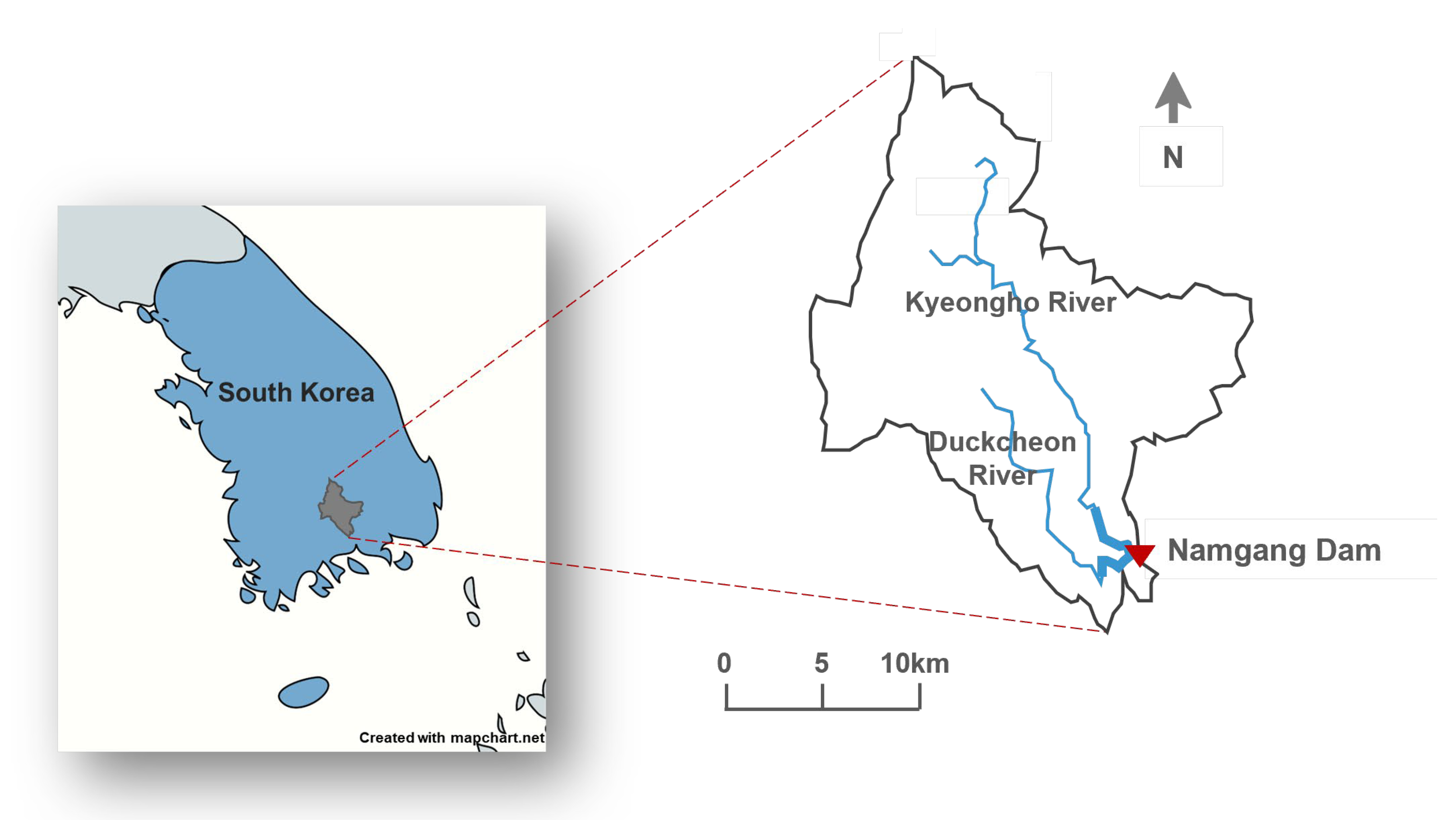
Figure 1. Location of the Namgang Dam basin in South Korea.
Water 17 03039 g001
Figure 2. Workflow of the proposed methodology for developing reservoir operation model.
Water 17 03039 g002
Figure 3. Reservoir volume–outflow relationship curve.
Water 17 03039 g003
Figure 4. Structure schematic of a GRU cell.
Water 17 03039 g004
Figure 5. Performance comparison of GRU-based reservoir operation models under various hyperparameter settings. (a) Batch size = 8; (b) Batch size = 32.
Water 17 03039 g005aWater 17 03039 g005b
Figure 6. Comparison of observed, optimized, and GRU-simulated reservoir outflows. (a) Flood event 2; (b) Flood event 5; (c) Flood event 7; (d) Flood event 12; (e) Flood event 16; (f) Flood event 17; (g) Flood event 20; (h) Flood event 25; (i) Flood event 34; (j) Flood event 37.
Water 17 03039 g006aWater 17 03039 g006bWater 17 03039 g006cWater 17 03039 g006dWater 17 03039 g006eWater 17 03039 g006f
Figure 7. Comparison of observed, optimized, and GRU-simulated reservoir storage levels. (a) Flood event 2; (b) Flood event 5; (c) Flood event 7; (d) Flood event 12; (e) Flood event 16; (f) Flood event 17; (g) Flood event 20; (h) Flood event 25; (i) Flood event 34; (j) Flood event 37.
Water 17 03039 g007aWater 17 03039 g007bWater 17 03039 g007cWater 17 03039 g007d
Table 1. Summary of flood event characteristics identified between 2000 and 2024.
EventPeriodDuration (hrs)Max
Inflow   ( m 3 / s )
Initial
Storage   ( 10 6 m 3 )
113 July 2000 10:0017 July 2000 22:00109652499.36
23 August 2000 14:005 August 2000 23:0058414978.56
312 September 2000 07:0019 September 2000 17:00179325870.41
424 June 2001 00:0026 June 2001 23:0072300978.92
55 July 2001 07:007 July 2001 08:00503364106.36
65 July 2002 04:007 July 2002 15:0060579231.59
76 August 2002 16:009 August 2002 23:0080544279.47
829 August 2002 09:002 September 2002 23:0011114,818149.45
911 September 2003 04:0015 September 2003 17:0011012,08258.12
1017 August 2004 10:0021 August 2004 13:00100607077.09
1121 August 2004 19:0025 August 2004 12:0090364175.69
128 July 2006 19:0013 July 2006 05:0010712,21482.15
137 August 2007 00:0011 August 2007 03:00100353445.49
1414 September 2007 09:0018 September 2007 22:001108792162.11
1514 July 2009 14:0019 July 2009 11:00118421190.88
1610 July 2010 21:0015 July 2010 00:00100354380.77
1715 July 2010 20:0020 July 2010 12:001133005157.65
1810 August 2010 03:0013 August 2010 23:00935846119.69
1916 August 2010 16:0019 August 2010 14:00714918155.85
201 September 2010 12:004 September 2010 01:00623857107.79
2125 June 2011 08:0029 June 2011 15:00104571178.30
228 July 2011 10:0012 July 2011 13:001007095123.76
237 August 2011 08:0010 August 2011 23:008810,648129.57
2421 August 2012 15:0027 August 2012 04:001343767127.14
2527 August 2012 22:0030 August 2012 12:00634895104.29
2616 September 2012 07:0019 September 2012 02:006814,101110.16
274 July 2013 12:007 July 2013 04:00654050116.40
282 August 2014 02:005 August 2014 23:00944898125.93
2911 July 2015 17:0014 July 2015 19:00754546114.95
3025 August 2018 17:0029 August 2018 05:00855257102.32
313 September 2018 16:005 September 2018 14:00473368150.23
325 October 2018 12:007 October 2018 17:00547433143.73
3319 July 2019 05:0023 July 2019 01:00933997144.25
342 October 2019 00:004 October 2019 15:00645784174.92
3512 July 2020 06:0014 July 2020 22:00655443167.71
3621 July 2020 22:0025 July 2020 22:00973492171.86
377 August 2020 01:009 August 2020 20:00688729165.78
382 September 2020 09:004 September 2020 11:0051621653.86
395 September 2022 13:007 September 2022 18:0054546748.97
4015 July 2023 11:0020 July 2023 17:00127393290.12
419 August 2023 14:0012 August 2023 02:0061479885.88
4229 August 2023 00:001 September 2023 20:00933658154.99
Table 2. Input variable configurations for scenario analysis.
ScenariosInput Variables
InflowStoragePrecipitation
1It−1St−1-
2It−1St−1Pt−1
3It−3, It−2, It−1St−3, St−2, St−1-
4It−3, It−2, It−1St−3, St−2, St−1Pt−3, Pt−2, Pt−1
5It−3, It−2, It−1, It, It+1, It+2St−3, St−2, St−1-
6It−3, It−2, It−1, It, It+1, It+2St−3, St−2, St−1Pt−3, Pt−2, Pt−1, Pt, Pt+1, Pt+2
Table 3. Data partitioning for GRU model training, validation and testing.
TrainingValidationTest
Event Max   Inflow   ( m 3 / s ) Event Max   Inflow   ( m 3 / s ) Event Max   Inflow   ( m 3 / s )
165244300924149
3325818584653364
6579219491875442
814,8182270951212,214
912,0822310,648163543
1060702614,101173005
113641294546203857
133534333997254895
148792363492345784
154211395467378729
215711423658386216
243767
274050
284898
305257
313368
327433
355443
403932
414798
Table 4. Hyperparameter configurations considered for tuning and optimization.
HyperparameterInterval
Window size[4, 6, 8]
Batch size[8, 32]
Number of hidden nodes[1, 100]
Table 5. RMSE and NSE values of GRU models for reservoir operation simulation.
ScenariosGRU HyperparametersRMSENSE
Batch SizeWindow SizeNumber of Hidden NodesTrainingValidationTestTrainingValidationTest
184100380.3411.2714.80.440.210.17
684364.0378.4712.70.490.340.18
854157.9202.1344.00.900.810.81
32490439.0417.8717.50.260.190.16
698137.9376.8671.00.930.340.27
884154.4251.6414.40.910.710.72
28460345.3397.1694.90.540.270.21
646360.9379.7690.40.500.330.23
822125.0294.5521.90.940.600.56
324100356.4396.9702.30.510.270.20
610356.6398.0700.50.510.260.20
854127.1355.9633.70.940.410.35
38426133.3118.5202.20.930.930.93
626155.8187.6310.90.910.840.84
814165.4174.5324.10.890.860.82
32462145.4204.6366.20.920.810.78
610163.2394.9679.00.900.280.26
816167.7216.8379.10.890.780.76
48420125.9160.7262.50.940.880.89
610155.6172.4250.20.910.860.90
810173.8226.0375.60.880.760.76
32446133.0202.5343.40.930.810.81
620153.4210.4366.80.910.790.78
812155.8240.6391.40.910.730.74
58424113.2160.2262.80.950.880.89
616144.7148.5261.70.920.900.89
812171.0170.3293.90.890.870.86
32420124.3160.9262.20.940.880.89
620143.8236.9435.90.920.740.69
824174.1187.0318.50.880.840.83
6841088.4299.4530.60.970.580.55
650123.2200.2323.90.940.810.83
824142.8213.3340.00.920.790.81
32414109.5249.2434.10.950.710.70
648124.8211.3340.10.940.790.81
840144.5225.9365.70.920.760.78
Disclaimer/Publisher’s Note: The statements, opinions and data contained in all publications are solely those of the individual author(s) and contributor(s) and not of MDPI and/or the editor(s). MDPI and/or the editor(s) disclaim responsibility for any injury to people or property resulting from any ideas, methods, instructions or products referred to in the content.