Abstract
Ensuring the quality of hydrological data is critical for effective flood forecasting, water resource management, and disaster risk reduction, especially in regions vulnerable to typhoons and extreme weather. This study presents a framework for quality control and outlier detection in rainfall and water level time series data using both supervised and unsupervised machine learning algorithms. The proposed approach is capable of detecting outliers arising from sensor malfunctions, missing values, and extreme measurements that may otherwise compromise the reliability of hydrological datasets. Supervised learning using XGBoost was trained on labeled historical data to detect known outlier patterns, while the unsupervised Isolation Forest algorithm was employed to identify unknown or rare outliers without the need for prior labels. This established framework was evaluated using hydrological datasets collected from Lao PDR, one of the member countries of the Typhoon Committee. The results demonstrate that the adopted machine learning algorithms effectively detected real-world outliers, thereby enhancing real-time monitoring and supporting data-driven decision-making. The Isolation Forest model yielded 1.21 and 12 times more false positives and false negatives, respectively, than the XGBoost model, demonstrating that XGBoost achieved superior outlier detection performance when labeled data were available. The proposed framework is designed to assist member countries in shifting from manual, human-dependent processes to AI-enabled, data-driven hydrological data management.
1. Introduction
The integrity and reliability of hydrological data, particularly rainfall and water level records, are essential for effective water resource management, flood forecasting, ecological assessment, and hydrological modeling. Traditional quality control (QC) procedures have long provided standardized methods to ensure data validity, as outlined in references such as the Hydrology Manual and the World Meteorological Organization’s (WMO) Quality Management Framework (QMF), which emphasize systematic validation and operational efficiency. However, the growing volume of telemetered data from precipitation and water level stations has highlighted the need for automation [1,2]. Recent advancements in artificial intelligence (AI) have enhanced data quality control by overcoming the limitations of conventional methods and improving detection of errors and outliers. Automated quality control (AQC) systems now enable consistent validation across large datasets, minimizing manual intervention and strengthening the overall reliability and usability of hydrological databases for scientific and operational applications [3,4].
Despite these advancements, hydrological data remain susceptible to various uncertainties and errors, stemming from measurement inaccuracies, environmental interferences, or data transmission issues. For example, the systematic review of flood prediction data highlights the challenges posed by uncertainties in rainfall data, which directly influence water flow and water level predictions [5]. These uncertainties necessitate robust QC mechanisms capable of detecting and correcting errors to improve the fidelity of hydrological models.
The detection of outliers in hydrological time series data such as rainfall and water level data is a critical aspect of water resource management, environmental monitoring, and disaster prevention. Recent advancements in machine learning (ML) techniques have significantly contributed to this domain, enabling more accurate and efficient identification of abnormal patterns. The following reviews synthesize findings from a range of studies that investigate the application of unsupervised and supervised machine learning algorithms for outlier detection in rainfall and water level datasets.
Unsupervised learning methods have been prominently utilized for pattern recognition and outlier detection without relying on labeled data. Autoencoders, a form of deep learning unsupervised model, have been employed for water level outlier detection with notable success. An example is the work on autoencoder-based outlier detection using time-series data, where the autoencoder reconstructs normal patterns and flags deviations as outliers [6]. This approach leverages the model’s ability to learn the normal behavior of water levels and identify outliers with high sensitivity. The use of autoencoders is particularly advantageous in streaming data scenarios, where real-time detection is essential [6]. In the context of rainfall data, the automatic quality control of crowdsourced rainfall measurements has been explored using both supervised and unsupervised algorithms. The study conducted on crowdsourced rainfall data revealed that unsupervised models could effectively identify outliers and inconsistencies, thereby improving data reliability [7]. The comparison between supervised and unsupervised techniques in this scenario underscores the flexibility of unsupervised methods in handling noisy and unstructured data, which is common in crowdsourced datasets [8].
Supervised learning approaches, on the other hand, require labeled datasets to train models to recognize outliers. Miau and Hung (2021) proposed a supervised deep learning framework for detecting abnormal water levels and river flooding events [9]. Their approach involved training models on labeled instances of normal and abnormal water levels, enabling precise classification and early warning capabilities. The advantage of supervised methods lies in their high accuracy when sufficient labeled data is available, as they can learn complex decision boundaries tailored to specific outlier types [9].
In summary, both supervised and unsupervised ML techniques have demonstrated significant potential in identifying abnormal rainfall and water level data. Unsupervised methods excel in scenarios with limited labeled data and are effective in discovering hidden patterns and outliers. Supervised approaches, particularly deep learning models like Autoencoders, provide high accuracy in classifying outliers when labeled datasets are available. The choice between supervised and unsupervised methods depends on data availability, the complexity of the environment, and specific application requirements. The reviewed literature underscores the versatility and effectiveness of ML models in identifying abnormal hydrological data. From traditional regression and classification models to advanced deep learning architectures and hybrid frameworks, ML techniques have demonstrated significant potential in improving outlier detection accuracy, enabling early warning systems by predicting river water levels and issuing early flood warnings several hours or days in advance using ML models trained on historical hydro-meteorological data, and supporting sustainable water resource management. The application of ML in quality controls of hydrological data has further enhanced the capacity for real-time monitoring and outlier detection, paving the way for more resilient hydrological systems in the face of climate variability and complicating water-related disasters and crisis.
In this study, an unsupervised Isolation Forest and a supervised XGBoost ML algorithm have been adopted to establish a framework for detecting outliers in hydrological datasets across Typhoon Committee (TC) member countries. Here, “outlier” refers to an observation in hydrological records that exhibits significant deviations from the expected range or the underlying statistical behavior of the dataset, potentially indicating an abnormal measurement or rare hydrological event. This initiative aims to enhance the capacity of TC members in implementing integrated hydrological data quality control and processing. Furthermore, this initiative is designed to assist member countries in shifting from manual, human-dependent processes to AI-enabled, data-driven hydrological data management. It is believed that this initiative can help address the shortage of experienced manpower in TC member countries by enabling a more holistic and automated approach to hydrological data management.
2. Study Area and Data Used
The TC Working Group on Hydrology (WGH) annually updates its Operational Plan to coordinate regional efforts in meteorology, hydrology, disaster risk reduction, and training related to typhoons. This plan, along with the Strategic Plan, guides the Committee’s activities and ensures a coordinated approach to reducing typhoon-related disasters in the Asia-Pacific region. Currently, there are nine on-going Annual Operation Plans (AOPs) under the WGH. The objective of this study is aligned with AOP2, under which the research project is entitled “Improvement of Hydrological Data Quality Control Systems Using AI Technology”. It also serves as an initiative to help authorities and practitioners in the selected member countries of Laos PDR, Malaysia, Philippines, and Thailand to switch from relying solely on manpower to digital approaches in managing hydrological data.
The Nam Ngum River Basin, located in Lao PDR, was selected as a testbed for developing a machine learning-based framework for detecting outliers in hydrological data as part of this demonstration study. Hydrological data were collected from four monitoring stations within the basin: Phiangluang, Thalad, Pakkayoung, and Veunkham. The Phiangluang station is situated in the upper reaches of the Nam Ngum River, while Thalad, Pakkayoung, and Veunkham are located downstream of the Nam Ngum Reservoir along the main river channel. Figure 1 presents the geographic distribution of these monitoring stations, which form the basis of the hydrological analysis conducted in this study. The coordinates for rainfall and water level measurements at each station are identical. Table 1 provides detailed metadata on the selected stations, and Table 2 summarizes key statistical characteristics of the hydrological variables. Among the stations, Veunkham, located furthest downstream near the confluence of the Nam Ngum and Mekong Rivers, recorded the highest annual average rainfall at 1651 mm. In contrast, Phiangluang, the most upstream station, recorded the lowest annual average rainfall at 1283 mm, yet experienced the highest single-day rainfall of 155.8 mm. The rainfall data used in this study represent daily cumulative values, while the water level data reflect daily average levels.
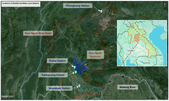
Figure 1.
Location of rainfall and water level stations in the Nam Ngum River Basin [10].

Table 1.
List of selected hydrological stations and respective locations.
Table 2.
Statistical values of hydrological variables for selected stations in Nam Ngum river basin [10].
In this study, daily rainfall and water level data from the four selected stations within the Nam Ngum River Basin are employed to train and validate the machine learning models adopted in outlier detection. The available data span the period from January 2019 to October 2021, with any intervals containing missing values excluded from the model training process. Table 3 presents a summary of data availability for the selected hydrological stations, while the corresponding time series plots are illustrated in Figure 2a–d. The hydrological datasets utilized in this study are consistent with those reported in [10].
Table 3.
Hydrological data availability at each monitoring station.
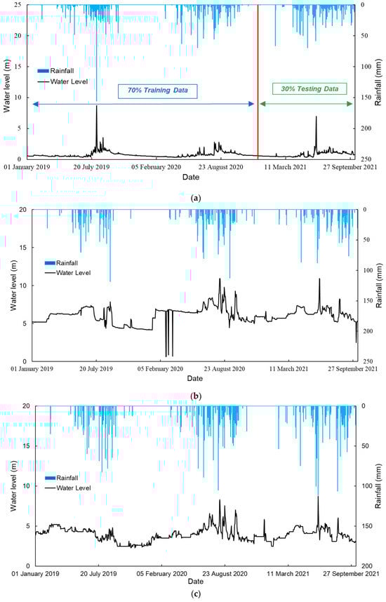
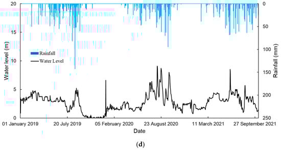
Figure 2.
(a). Time series plot for hydrological data collected at Phiangluang station. (b). Time series plot for hydrological data collected at Thalad station. (c). Time series plot for hydrological data collected at Pakkayoung station. (d). Time series plot for hydrological data collected at Veunkham station.
3. Methodology
3.1. Unsupervised Learning-Isolation Forest
The main advantage of using an unsupervised machine learning algorithm for outlier detection is that it does not require labeled datasets to train a model to identify whether a hydrological data point is normal or abnormal. This makes an unsupervised machine learning algorithm a powerful surrogate model for screening out abnormal hydrological data, especially contexts when no labeled datasets are available. Moreover, Halicki et al. (2024) [11] reported that the majority of unsupervised machine learning algorithms are non-parametric, meaning they do not assume that the underlying dataset follows any specific statistical distribution. This makes them particularly suitable for real-world applications where data often exhibit complex, non-normal patterns. Isolation Forest (IF) is an algorithm that was originated by Liu and Zhou (2008) [12] that employs binary trees to identify outliers, resulting in a linear time complexity and low memory usage that is appropriate for processing large datasets as well.
Isolation Forest (IF) is based on the main principle that abnormal data points are scarce and highly distinguishable in a time series. In an Isolation Forest, randomly sub-sampled data are processed through a tree structure built using randomly selected features. The algorithm isolates observations by recursively partitioning the data. Samples that travel deeper into the tree require more splits to be isolated, indicating that they are more similar to the rest of the data and thus less likely to be outliers. In contrast, samples that appear on shorter branches are isolated with fewer cuts, suggesting that they are outliers, as it is easier for the tree to separate them from the majority of observations.
As noted previously, Isolation Forest is an ensemble-based method for outlier detection, consisting of multiple binary decision trees. Each individual tree within the Isolation Forest is referred to as an Isolation Tree (iTree). When a dataset is provided to the Isolation Forest (IF) model, a random sub-sample of the data is first selected and used to construct a binary decision tree, iTree. The tree grows by recursively selecting a feature at random from the available N features. A random threshold value is then chosen within the range of the selected feature’s minimum and maximum values. For each node, the data is split based on this threshold: if a data point’s feature value is less than the threshold, it is directed to the left branch; otherwise, it goes to the right branch. In this way, each node creates a binary split of the data. This recursive partitioning continues until either each data point is completely isolated in a leaf node, or a predefined maximum depth is reached. The process described above is repeated multiple times to build a forest of random binary trees, where each tree contributes to evaluating how easily individual points can be isolated.
During the scoring phase, each data point is passed through all the trained trees in the forest. The model calculates an outlier score for each point based on the average path length, that is, the number of splits (tree depth) required to isolate the point across all trees. Points that are isolated quickly (i.e., with shorter path lengths) are likely to be outliers, as fewer conditions are needed to separate them from the rest of the data. In contrast, normal points tend to have longer path lengths due to their similarity to many other observations. The final outlier score is a normalized function of the average path length, and it typically ranges between 0 (most normal) and 1 (most anomalous). A threshold based on the contamination parameter—which specifies the expected proportion of outliers in the dataset—is used to classify each point. Often, a score close to 1 indicates an outlier, while a score closer to 0 indicates a normal point.
The mathematical expressions which are used to calculate the outlier score s(x,n) based on the path length of a data point in the tress can be found in Equations (1)–(4):
where n is the number of samples used to build each tree, c(n) indicates the normalization factor, which represents the average path length of unsuccessful searches in Binary Search Tree (BST) of n points, H(i) informs the harmonic number with as Euler constant of approximately 0.5772, and ht(x) denotes the path length in each tree, t. It has been reported in [11] that the only drawback of IF is that the users need to specify the contamination parameter manually; the specified value sets the decision threshold where, when the ranks of outlier score data points exceed the specified contamination level, they are labeled as outliers. In other words, a contamination level of 0.01 means that 1% of the data will be treated to be anomalous.
3.2. Supervised Learning-XGBoost
XGBoost (eXtreme Gradient Boosting) is an open-source machine learning algorithm, introduced by Chen (2016) [13] and widely used for training classification and regression models. It is primarily applied to supervised learning problems, where input features xi are used to predict a target variable yi. XGBoost has also been successfully adopted for quality control and outlier detection in hydrological time series, provided that sufficient labeled data is available.
As a supervised learning model, XGBoost learns from historical labeled datasets. In the context of outlier detection, it builds an ensemble of decision trees using gradient boosting, where each tree identifies patterns that distinguish between normal and abnormal instances in the hydrological data. This requires a labeled training dataset consisting of input variables (e.g., rainfall or water level time series) and corresponding class labels. Typically, a label of 0 denotes normal data and 1 denotes abnormal data, or vice versa.
During training, XGBoost minimizes classification errors by assigning greater weight to instances that were previously misclassified. This iterative process continues until a strong predictive model is constructed. XGBoost is capable of learning complex non-linear relationships and interactions among features, making it particularly effective at detecting subtle outliers. When new or unlabeled data is introduced to the trained model, it passes through the ensemble of trees. The model then produces an output—either a probability or a binary classification—indicating whether the input is normal or abnormal.
The core mathematical foundations of XGBoost can be expressed as it predicts an output as the sum of K regression trees:
where fk are functions from the space of regression trees. Then, XGBoost optimizes a regularized objective function () as depicted in Equations (6)–(7) that balances model fit and complexity:
where l is a differentiable loss function and function in Equation (7) penalizes complexity, with T being the number of leaves and w being their weights on leaves, while are just the regularization parameters. The objective is consequently approximated at each boosting iteration by using a second-order Taylor expansion, as presented in Equation (8):
where gi and hi are the first and second derivatives of the loss function with respect to previous predictions. The optimal weight for each leaf is then achieved through Equation (9), and the best tree structure minimizes the regularized loss using these weights.
where Ij represents the set of instances in leaf j. These mathematically efficient frameworks make XGBoost both powerful and effective at maximizing the separation between normal and abnormal patterns through gradient-based optimization and tree-based splits, making it a popular machine learning model for outlier detection in hydrological data. The outlier detection codes based on the Isolation Forest and XGBoost algorithms in this study were developed in Python (version 3.10.12) within the Spyder modeling environment (version 5.4.3).
No normalization or scaling was applied to the hydrological datasets prior to model training. This is appropriate because both the Isolation Forest (sklearn.ensemble) and XGBoost (xgboost) models are tree-based or partition-based, and therefore insensitive to feature scales. As a result, differences in the magnitude of input features do not affect the model’s ability to detect outliers in the data. Apart from that, both models were run with their default hyperparameter settings as provided in these libraries.
3.3. Thresholds for Outlier Classification in Labeled Datasets
In the previous section, it was elaborated that labeled datasets are essential for applying XGBoost as a supervised learning method for detecting outliers in hydrological time series data. Therefore, a standard or boundary must be defined to distinguish abnormal data from normal data, enabling each data point to be labeled accordingly. In this study, the hydrological data which is comprising daily rainfall and water level will be validated based on four major criteria: (1) statistical checks (e.g., minimum and maximum thresholds), (2) slope checks (e.g., abnormal rates of increase or decrease), (3) duration checks (e.g., prolonged constant or missing values), and (4) spatial checks (e.g., inconsistency with neighboring stations).
3.3.1. Statistical Check (Minimum/Maximum Values)
The statistical check involves validating hydrological data by comparing each data point against predefined statistical thresholds to detect outliers or physically implausible values. This process is grounded in the assumption that normal hydrological behavior follows certain statistical patterns that can be characterized by historical observations or climatological norms. The statistical check usually serves as the first line of defense in data validation, helping to identify errors that are extreme or physically implausible before more complex temporal or spatial analyses are performed.
Hubbard et al. [14] proposed the use of statistical boundaries based on the mean and standard deviation of historical rainfall data to identify potential abnormal data or outliers. This approach was adopted in this study by computing the statistical boundaries using the historical daily rainfall data in available years, excluding non-precipitation (zero rainfall) days. A similar methodology was applied to the water level data, except both minimum and maximum outliers were evaluated and zero observations were included for computing the boundaries in water level. The validation boundaries adopted for statistical check are summarized in Table 4.
Table 4.
Validation boundaries for labeled datasets in statistical check.
The potential abnormal data were detected according to the conditions stated in Equation (10) for statistical checking of the hydrological data.
where TST,min and TST,max indicate the lower and upper validation boundary for the desired hydrological data where a data point, Xt, that was located within the boundary was classified as normal data, while it was recognized as potential abnormal data when it was located beyond the specified boundary (where , is the mean and standard deviation of observed rainfall or water level).
3.3.2. Slope (Rate of Change Ratio)
The slope check is designed to detect unrealistic or abrupt changes in hydrological time series data, such as sudden jumps or drops in values that are inconsistent with the physical behavior of the environment or the expected response of the measurement system. It evaluates the rate of change (i.e., the slope) between consecutive data points to identify outliers that may result from sensor errors, data transmission faults, or manual entry mistakes. The slope check on hydrological time series data enhances the robustness of outlier detection by focusing on the dynamic behavior of the data, rather than just the magnitude. It is especially useful in combination with the statistical and duration checks to capture a wider range of error patterns. The validation boundaries adopted for slope check of water level data are summarized in Table 5.
Table 5.
Validation boundaries for labeled datasets in slope check.
The potential abnormal data were detected according to the conditions stated in Equation (11) for slope checking of the water level data.
where TSL,max indicates the upper validation boundary for the rate of change ratio, Rt in both increasing and decreasing slopes. The Korea Institute of Civil Engineering and Building Technology (KICT) [15] recommend using the rate of change ratio to determine the water level fluctuation boundary, where the ratio was computed by dividing the slope at one time step prior by the slope at two time steps prior based on the formula shown in Equation (12). Only non-zero values and the absolute values of the computed ratios were used in determining the threshold boundary (where , is the mean and standard deviation of ratio computed in increasing and decreasing slope respectively) as depicted in Table 5. A data point with ratio Rt exceeding the specified boundary was flagged as potential abnormal data.
3.3.3. Duration Check
The duration check is a time-based validation method used to identify abnormal persistence or repetition in hydrological time series data, such as unrealistically long periods of unchanged or missing values. While some hydrological conditions may naturally remain stable for short durations (e.g., dry spells with zero rainfall), extended durations of identical or missing values often indicate sensor malfunction, data transmission failure, or erroneous data entry. The duration check is particularly effective in detecting sensor freezes, manual data entry errors, and missing transmission blocks, making it an essential component of a robust hydrological data quality control system. The validation boundaries adopted for duration check of constant water level data are summarized in Table 6.
Table 6.
Validation boundaries for labeled datasets in duration check.
The potential abnormal data were detected according to the conditions stated in Equation (15) for duration checking of the constant water level data.
where TD,max indicates the upper validation boundary for the duration with constant water level, Dt. A data point with Dt (the total accumulated number of days with unchanged water level, where , is the mean and standard deviation of Dt) exceeding the specified boundary was flagged as potential abnormal data.
3.3.4. Spatial Check
The spatial check is a quality control method that evaluates the consistency of a station’s hydrological data by comparing it with observations from neighboring or hydrologically similar stations. The underlying principle is that nearby stations within the same climatic and hydrological region should exhibit similar patterns, especially for short-term variations such as rainfall events or water level responses to regional precipitation. Deviations from these expected spatial patterns may indicate outliers due to instrument malfunction, data corruption, or localized errors.
The spatial check is particularly effective in detecting localized sensor malfunctions, extreme outliers, or systematic errors (e.g., shifted or corrupted time stamps). It complements the temporal-based checks (statistical, slope, and duration) by leveraging the spatial redundancy inherent in hydrological monitoring networks. The validation boundaries adopted for spatial check of rainfall data are summarized in Table 7.
Table 7.
Validation boundaries for labeled datasets in spatial check.
The Korea Water Resources Corporation (K-water) [16] in the Republic of Korea proposed a spatial validation boundary based on the difference (RDSdiff) between the observed rainfall at the target station and the rainfall predicted by the RDS (Reciprocal Distance Squared) method, XRDS using observed rainfall from the selected neighboring stations. The RDS method is a spatial reconstruction approach based on the concept that the spatial correlation of precipitation decreases with increasing physical distance. Using this method, the reconstructed precipitation at a target station can be estimated from observations at two or more nearby stations, as described in Equation (16).
where XRDS,t is the rainfall value reconstructed at the target station at time, t using the RDS approach, while Xt,i is the observed rainfall at nearby i-th station at time, t, di is the corresponding distance between the target station and the nearby i-th station, and m is the total number of selected nearby stations used for computing the reconstructed rainfall in RDS. The difference (RDSdiff) between the observed rainfall at the target station and the predicted RDS rainfall at time t was then computed according to Equation (17). TSP,min and TSP,max represent the lower and upper validation boundaries, respectively. An observed rainfall value at the target station at time, t was classified as normal if the relative difference from the RDS computed rainfall fell within this range. If the difference exceeded these boundaries, the data point was flagged as potential abnormal data.
4. Results and Discussions
4.1. Outlier Detection in Statistical Check
Maximum rainfall outliers and minimum/maximum water level outliers for the selected stations were identified using the unsupervised Isolation Forest algorithm and the supervised XGBoost algorithm, as described in the previous section. The threshold values that distinguish the normal from abnormal data in unsupervised approach were based on contamination levels specified for each station, while in the supervised approach, they were computed using the equations as elaborated in Section 3.3.1. In the supervised learning process, 70% of the time series data were used to train the XGBoost model, and the remaining 30% were reserved for testing (as illustrated in Figure 2a).
In this study, the Isolation Forest model was applied in a purely unsupervised manner for anomaly detection, where no labeled data or train–test split was used for model training. The primary objective was to detect anomalies within the entire hydrological time series rather than to perform predictive evaluation. Therefore, the model was trained on the full dataset to learn the overall data distribution and identify potential outliers accordingly. Since no ground truth labels were used during training or threshold calibration, this approach does not introduce data contamination. Therefore, train–test split was not required in unsupervised learning. It should be noted that, since the evaluation labels were derived from the same threshold rules described in Section 3.3, the assessment may involve a certain degree of circular validation, which is acknowledged as a limitation of this study.
To evaluate the performance of both machine learning models in detecting outliers in the hydrological time series, abnormal data identified using the threshold criteria defined in the previous section were treated as the ground truth. The Isolation Forest and XGBoost models were then assessed based on their ability to capture these reference outliers. The classification results and confusion matrices for outlier detection using the Isolation Forest and XGBoost models at each station are summarized in Table 8, Table 9, Table 10 and Table 11.
Table 8.
Results of classifications for outlier detection of maximum rainfall using unsupervised Isolation Forest model.
Table 9.
Summary of confusion matrices for outlier detection of maximum rainfall using unsupervised Isolation Forest model.
Table 10.
Results of classifications for outlier detection of maximum rainfall using supervised XGBoost model.
Table 11.
Summary of confusion matrices for outlier detection of maximum rainfall using supervised XGBoost model.
Performance metrics such as precision, recall, and F1-score were used to evaluate the model’s ability to capture abnormal maximum rainfall events. Precision measures the proportion of predicted outliers that are truly outliers, reflecting the model’s ability to avoid false alarms. Recall measures the proportion of actual outliers correctly identified, indicating how well the model detects all true outliers. The F1-score is the harmonic mean of precision and recall, providing a balanced assessment of both aspects. In outlier detection, high precision means most predicted outliers are correct, while high recall means the model successfully finds all actual outliers. A precision and recall (and thus F1-score) of 1.0 indicate perfect detection, no false positives and no false negatives, meaning the model detected every outlier, and all detections were correct.
It can be observed in Table 8 that with a contamination level of 0.005, the Isolation Forest model achieved perfect outlier detection (recall = 1.00) across stations but exhibited reduced precision due to false positives (Table 9), indicating over-prediction of outliers in most of the stations except for Phiangluang station. However, the XGBoost model performed poorly in maximum rainfall outlier detection where the true outliers were only successfully found at Phiangluang and Veunkham stations according to the classification results and confusion matrices presented in Table 10 and Table 11. No outliers were detected at Thalad and Pakkayoung stations. This low detection rate may be attributed to the limited number of true outliers in the rainfall time series (only two in the training period), which likely hindered the model’s ability to learn the underlying outlier patterns during training, resulting in failure to detect them in the testing period. The maximum rainfall outliers identified at station Phiangluang by both the Isolation Forest and XGBoost models are demonstrated in Figure 3 and Figure 4.
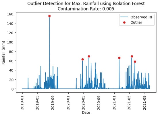
Figure 3.
Maximum rainfall outliers identified at station Phiangluang using Isolation Forest model.
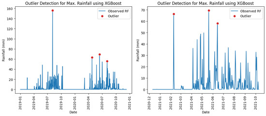
Figure 4.
Maximum rainfall outliers identified at station Phiangluang using XGBoost model in training (left) and testing (right) periods.
Both minimum and maximum water level outliers were identified using the same approach applied for maximum rainfall outliers, as described in the previous paragraph. The classification results and confusion matrices for water level outlier detection are presented in Table 12, Table 13, Table 14 and Table 15. As shown in Figure 5 and Figure 6, both the Isolation Forest and XGBoost models successfully captured the minimum and maximum water level outliers. However, the Isolation Forest’s ability to detect minimum water level outliers was strongly influenced by the shape of the left tail in the observed water level distribution.
Table 12.
Results of classifications for outlier detection of minimum and maximum water level using unsupervised Isolation Forest model.
Table 13.
Summary of confusion matrices for outlier detection of minimum and maximum water level using unsupervised Isolation Forest model.
Table 14.
Results of classifications for outlier detection of minimum and maximum water level using supervised XGBoost model.
Table 15.
Summary of confusion matrices for outlier detection of minimum and maximum water level using supervised XGBoost model.
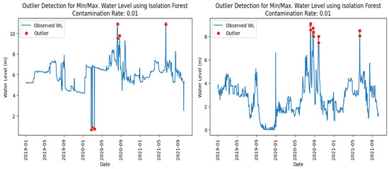
Figure 5.
Minimum/maximum water level outliers identified at station Thalad (left) and Veunkham (right) using Isolation Forest model.
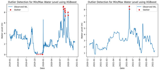
Figure 6.
Minimum/maximum water level outliers identified at station Veunkham using XGBoost model in training (left) and testing (right) periods.
The classification results in Table 12 indicate that the Isolation Forest achieved high recall rates at most stations for detecting water level outliers at a contamination level of 0.01, except for at the Veunkham station. Figure 7 shows the distribution of observed water levels for station Veunkham during the training and testing periods. In the training period, the left tail of the distribution exhibited a sharp spike at zero values. This likely explains why these extreme values were not identified as minimum water level outliers by the Isolation Forest (Figure 5, right). Since the model learned that such zero values were common rather than unique, it did not isolate them as outliers. Consequently, the recall rate for station Veunkham was low, as the model failed to classify the zero water level values as outliers.
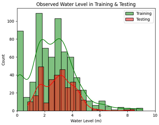
Figure 7.
Histogram for distribution of observed water level at station Veunkham in training and testing periods (The solid lines indicate Kernel Density Estimation in training and testing periods).
The XGBoost model consistently outperformed the Isolation Forest in detecting both minimum and maximum water level outliers, achieving high performance metrics across all stations, as summarized in Table 14. Unlike its relatively poor performance in detecting maximum rainfall outliers, the XGBoost model yielded promising results for both minimum and maximum water level outliers. This demonstrates that the performance of a supervised learning algorithm can be significantly enhanced when sufficient labeled datasets are available, which was further proven by the low counts of false positives and false negatives obtained from the XGBoost model, as reported in Table 15.
4.2. Outlier Detection in Slope (Ratio of Change) Check
The slope (ratio of change) check was applied exclusively to the water level time series to detect outliers caused by abrupt changes in water level. In this method, the water level at the current time step was compared with the previous two time steps, and any change exceeding the threshold defined in Section 3.3.2 was classified as an outlier. The slope, or ratio of change, was calculated by dividing the difference between the current water level and that of one time step earlier by the difference between the water level at one time step earlier and that of two time steps earlier. Positive slopes indicate an increasing water level trend, while negative slopes indicate a decreasing trend at the current time step. This derived slope (ratio of change) series was then input into the Isolation Forest and XGBoost models to identify potential abrupt change outliers. Any observed water level associated with a slope or ratio of change value exceeding the specified threshold was flagged as a potential outlier. The classification results and confusion matrices for each station using the Isolation Forest and XGBoost models are summarized in Table 16, Table 17, Table 18 and Table 19.
Table 16.
Results of classifications for outlier detection of abrupt water level change using unsupervised Isolation Forest model.
Table 17.
Summary of confusion matrices for outlier detection of abrupt water level change using unsupervised Isolation Forest model.
Table 18.
Results of classifications for outlier detection of abrupt water level change using supervised XGBoost model.
Table 19.
Summary of confusion matrices for outlier detection of abrupt water level change using supervised XGBoost model.
The classification results in Table 16 show that almost all outliers detected by the Isolation Forest model at a contamination level of 0.02 were true outliers, as evidenced by precision scores of 1.00 across all stations except for station Thalad. However, the model failed to capture all true outliers at this setting due to low recall rates in most stations. Recall could likely be improved by increasing the contamination level, as the actual number of outliers in several stations exceeded 20, whereas the current setting of 0.02 isolates only about 20 out of 1014 data points, leading to an underestimation of outliers. In contrast, the XGBoost model effectively identified the actual constant water level outliers, achieving consistently higher precision and recall scores across all stations, as reported in Table 18. Figure 8 and Figure 9 illustrate the detection of abrupt water level change outliers at station Thalad using the Isolation Forest and XGBoost models. The visual patterns are consistent with the classification results and confusion matrices in the tables, with red dots (representing outliers) appearing at points corresponding to sudden spikes or plunges in water level.
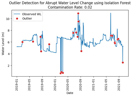
Figure 8.
Abrupt water level change outliers identified at station Thalad using Isolation Forest model.
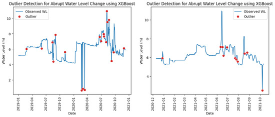
Figure 9.
Abrupt water level change outliers identified at station Thalad using XGBoost model in training (left) and testing (right) periods.
4.3. Outlier Detection in Duration Check
The duration check was applied only to the water level time series to identify outliers caused by constant water levels. In this approach, observations were classified as abnormal when their values remained unchanged for periods exceeding the threshold defined in Section 3.3.3. For each station, the total accumulated number of consecutive days with unchanged water level (Dt) was calculated from the observed time series. This derived Dt series was then input into the Isolation Forest and XGBoost models to detect potential constant water level outliers. Any observed water level associated with a Dt value exceeding the specified threshold was flagged as a potential outlier. The classification results and confusion matrices for outlier detection using the Isolation Forest and XGBoost models at each station are summarized in Table 20, Table 21, Table 22 and Table 23.
Table 20.
Results of classifications for outlier detection of constant water level using unsupervised Isolation Forest model.
Table 21.
Summary of confusion matrices for outlier detection of constant water level using unsupervised Isolation Forest model.
Table 22.
Results of classifications for outlier detection of constant water level using supervised XGBoost model.
Table 23.
Summary of confusion matrices for outlier detection of constant water level using supervised XGBoost model.
The classification results in Table 20 indicate that all outliers detected by the Isolation Forest model at a contamination level of 0.01 were true outliers, as evidenced by precision scores of 1.00 across all stations. However, the unsupervised model failed to capture all true outliers at this contamination level due to low recall rates at most stations, as well as high counts of false negatives, as summarized in Table 21. For stations Phiangluang, Thalad, and Pakkayoung, recall could likely be improved by increasing the contamination level from 0.01 to 0.03. At these stations, the actual number of outliers exceeded 30, whereas the current contamination setting of 0.01 isolates only about 10 out of 1014 data points, resulting in an underestimation of outliers. In contrast, the XGBoost model successfully captured all actual constant water level outliers, achieving both precision and recall scores of 1.00 across all stations, as reported in Table 22. Apart from that, zero count of false positives and false negatives was also achieved by XGBoost, as summarized in Table 23. This further supports the earlier conclusion that a supervised model can perform highly effectively in outlier detection when provided with sufficient labeled datasets.
Figure 10 and Figure 11 illustrate the detection of constant water level outliers at station Thalad using the Isolation Forest and XGBoost models. The observations align with the classification results in Table 20, Table 21, Table 22 and Table 23, showing that the number of red dots (representing outliers) identified by the Isolation Forest was lower than that identified by XGBoost. Additionally, the threshold applied in the Isolation Forest at a contamination level of 0.01 appeared higher, as only short periods of data were flagged as abnormal, whereas the XGBoost model recognized longer periods as potential outliers. In other words, a higher threshold computed in Isolation Forest resulted in fewer data points being classified as outliers, since the model required a greater total accumulated number of consecutive days with unchanged water levels to distinguish abnormal from normal conditions.
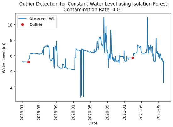
Figure 10.
Constant water level outliers identified at station Thalad using Isolation Forest model.
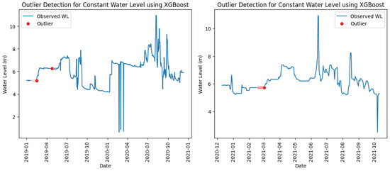
Figure 11.
Constant water level outliers identified at station Thalad using XGBoost model in training (left) and testing (right) periods.
4.4. Outlier Detection in Spatial Check
The spatial check was applied exclusively to the rainfall time series to detect outliers arising from significant differences between the target station rainfall and the corresponding RDS rainfall. In this method, rainfall observed at the target station was classified as abnormal when its difference from the RDS rainfall exceeded the threshold defined in Section 3.3.4. For each target station, the difference was calculated by subtracting the target station rainfall from the RDS rainfall computed from a neighboring rainfall station. This derived rainfall difference/residual series was then input into the Isolation Forest and XGBoost models to detect potential significant rainfall difference outliers. Any rainfall values at the target station associated with a difference value exceeding the specified threshold was flagged as a potential outlier. The classification results and confusion matrices for outlier detection using the Isolation Forest and XGBoost models at each station are summarized from Table 24, Table 25, Table 26 and Table 27.
Table 24.
Results of classifications for outlier detection of rainfall spatial check using unsupervised Isolation Forest model.
Table 25.
Summary of confusion matrices for outlier detection of rainfall spatial check using unsupervised Isolation Forest model.
Table 26.
Results of classifications for outlier detection of rainfall spatial check using supervised XGBoost model.
Table 27.
Summary of confusion matrices for outlier detection of rainfall spatial check using supervised XGBoost model.
The classification results and confusion matrices in Table 24, Table 25, Table 26 and Table 27 indicate that both Isolation Forest and XGBoost models performed equally good at detecting outliers for rainfall spatial check, as evidenced by precision and recall scores of close to 1.0 and low counts of false positives and false negatives across all stations. Figure 12 shows the detection of rainfall spatial check outliers at station Pakkayoung using the Isolation Forest model at a contamination level of 0.05, while Figure 13 demonstrates the results obtained from XGBoost. The RDS rainfalls computed from neighboring stations are also indicated in the figures, as an orange line. It was observed that almost all similar red dots (representing outliers) have been successfully captured in both unsupervised and supervised learnings.
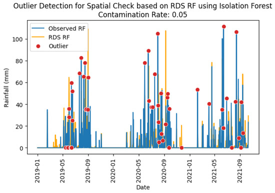
Figure 12.
Rainfall spatial check outliers identified at station Pakkayoung using Isolation Forest model.
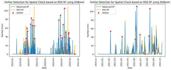
Figure 13.
Rainfall spatial check outliers identified at station Pakkayoung using XGBoost model in training (left) and testing (right) periods.
As discussed earlier, the performance of the Isolation Forest model is highly dependent on the shape of the data distribution, particularly the left and right tails. The bell-shaped distribution of the differences between target rainfall and RDS rainfall, as shown in Figure 14, explains the excellent performance of the model in detecting outliers during the rainfall spatial check. In Figure 14, positive and negative residuals indicate overestimation and underestimation of the target station rainfall relative to the corresponding RDS rainfall. The absence of sharp spikes in both tails allowed the Isolation Forest to readily identify and isolate data beyond the lower (left tail) and upper (right tail) thresholds as outliers.
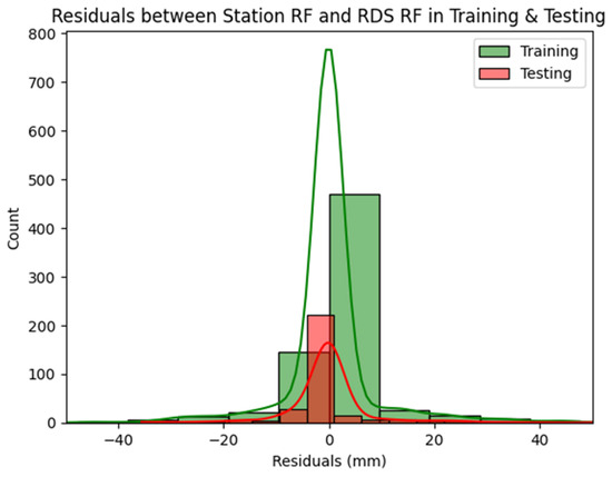
Figure 14.
Histogram for distribution of differences between target rainfall and RDS rainfall at station Pakkayoung in training and testing periods (The solid lines indicate Kernel Density Estimation in training and testing periods).
4.5. Synthesis of Outlier Detection Results from Unsupervised and Supervised Learning Approaches
The unsupervised Isolation Forest and supervised XGBoost algorithms were applied for outlier detection in hydrological time series data in Lao PDR. Their performances in each detection category—statistical check, duration check, slope (ratio of change) check, and spatial check—have been discussed in detail in the preceding sections. The results show that both approaches have distinct advantages and limitations. Practitioners in TC member countries may select the approach most suitable for their specific site conditions and data availability. Table 28 summarizes the key strengths and weaknesses of each approach as applied in this study.
Table 28.
Summary of merits and demerits of the Isolation Forest and XGBoost models for outlier detection in hydrological time series.
In summary, the choice between Isolation Forest and XGBoost for outlier detection in hydrological time series should be guided by the availability of labeled data, the characteristics of the dataset, and the operational context. Isolation Forest offers a practical solution when labeled outliers are scarce, making it particularly useful for stations with limited historical records or where manual labeling is not feasible. However, its sensitivity to data distribution, especially in the tails, necessitates careful parameter tuning to achieve balanced performance. In contrast, XGBoost demonstrated superior and more consistent performance when sufficient labeled data were available, exhibiting greater resilience across different outlier categories and less dependency on distributional characteristics. This is supported by the fact that XGBoost was able to capture the constant water level and abrupt change outliers missed by Isolation Forest at Thalad station. The Isolation Forest model produced 1.21 and 12 times more false positives and false negatives, respectively, than XGBoost, as depicted in Table 29, further confirming XGBoost’s effectiveness in outlier detection under labeled data conditions. Therefore, a hybrid strategy employing the Isolation Forest as an initial screening tool and applying XGBoost for fine-tuned classification where labeled data are available is recommended for TC member countries to maximize detection accuracy while accommodating diverse data conditions.
Table 29.
Summary of false counts.
Figure 15 illustrates the schematic framework proposed for hydrological data quality control in TC member countries. In the present study, stage 1 of the framework is addressed, where the machine learning methods Isolation Forest and XGBoost were employed to detect outliers in hydrological data. Stage 2, which will be the focus of future work, involves correcting the detected outliers using AI techniques such as LSTM Autoencoders. This two-stage approach aims to establish a comprehensive AI-based system for hydrological data quality control across TC member countries.
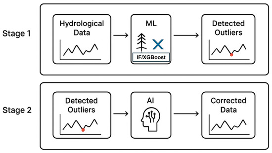
Figure 15.
Schematic framework for hydrological data quality control in TC member countries.
Future work should focus on developing hybrid ML frameworks that combine the strengths of both data-driven and physically based hydrological models for more robust outlier detection. Integrating Explainable AI (XAI) techniques, such as SHAP or LIME, can enhance the interpretability of model decisions and increase trust among hydrologists and practitioners. These approaches would allow for the identification of not only anomalous values but also their underlying causes, such as sensor faults or extreme events. Ultimately, hybrid and explainable ML systems could improve the transparency, accuracy, and operational reliability of automated hydrological data quality control.
Apart from that, although the present study demonstrates the feasibility of using Isolation Forest and XGBoost for hydrological outlier detection, aspects such as computational efficiency, scalability to large datasets, and practical integration into national hydrological services were not evaluated. Future work should also address these dimensions, including optimizing model runtimes, assessing performance across multiple stations, and developing procedures for operational integration into existing data quality control and flood forecasting systems. Addressing these factors is essential to ensure that machine learning models can be deployed effectively in real-world hydrological monitoring and decision-making workflows.
5. Conclusions
This study evaluated the performance of unsupervised (Isolation Forest) and supervised (XGBoost) algorithms for outlier detection in hydrological time series collected in Lao PDR, focusing on rainfall and water level data. Outliers were detected through statistical, duration, slope (ratio of change), and spatial checks, addressing various hydrological behaviors such as extreme values, constant water levels, abrupt changes, and spatial inconsistencies. The results indicate that both approaches offer distinct advantages and limitations. Isolation Forest, which does not require labeled data, effectively captured minimum and maximum outliers in water level and rainfall series, particularly when the data distributions were favorable and tail behaviors were moderate. In spatial checks with normally distributed residuals, the model reliably identified outliers. However, its performance was highly sensitive to distribution shapes and contamination levels. For instance, stations with frequent extreme values, such as zero water levels at Veunkham, exhibited low recall, and low contamination levels led to underestimation of outliers.
XGBoost performed better for detection of water level outliers, but less effectively for rainfall outliers with sparse true positives. Specifically, the Isolation Forest model generated 1.21 and 12 times more false positives and false negatives, respectively, than XGBoost, highlighting the superior outlier detection capability of XGBoost under labeled data conditions. The XGBoost model successfully identified minimum and maximum water level outliers, as well as outliers from duration and slope checks, demonstrating robustness across stations and less dependence on data distribution. Its supervised nature, however, limits applicability in datasets lacking representative labeled outliers. Visual analyses supported these findings. For example, XGBoost captured constant water level and abrupt change outliers missed by Isolation Forest at Thalad. In rainfall spatial checks, both models performed well when distributions were favorable, but the performance of Isolation Forest degraded in distributions with heavy tails. Based on these observations, a hybrid approach is recommended: using Isolation Forest as an initial screening tool for unlabeled datasets, followed by XGBoost for fine-tuned classification where labels exist. This strategy maximizes detection accuracy while accommodating diverse data conditions.
Overall, integrating unsupervised and supervised learning provides a flexible and effective framework for hydrological outlier detection, supporting data quality assurance, real-time monitoring, and water resource management. The study highlights the importance of considering data characteristics, distribution shapes, and parameter settings when applying these algorithms, offering practical guidance for TC member countries and future hydrological studies.
Author Contributions
Conceptualization, C.-S.K. and C.-R.K.; methodology, K.-H.K. and C.-S.K.; software, K.-H.K.; validation C.-S.K. and C.-R.K.; formal analysis, K.-H.K. and C.-S.K.; investigation, K.-H.K.; resources, C.-S.K. and C.-R.K.; data curation, K.-H.K.; writing—original draft preparation, K.-H.K.; writing—review and editing, C.-S.K. and C.-R.K.; visualization, K.-H.K.; supervision, C.-S.K. and C.-R.K.; project administration, C.-S.K. and C.-R.K.; funding acquisition, C.-S.K. All authors have read and agreed to the published version of the manuscript.
Funding
This research was funded by Ministry of Environment of Republic of Korea under the grant title of “Enhancing the Flood Management Framework for Member Countries in Typhoon Committee (2nd Phrase) (Grant No: 20250464-001)”.
Data Availability Statement
The data presented in this study are available upon request from the corresponding author. The data are not publicly available due to not having a public repository at the time of this publication.
Conflicts of Interest
The authors declare no conflicts of interest.
References
- Los Angeles County Department of Public Works. Hydrology Manual; Water Resources Division, Los Angeles County Department of Public Works: Alhambra, CA, USA, 2006.
- WMO. Guidelines on Surface Station Data Quality Control and Quality Assurance for Climate Applications; WMO-No. 1269; World Meteorological Organization: Geneva, Switzerland, 2021. [Google Scholar]
- Zhou, R.D.; Seong, Y.U.; Liu, J.P. Review of the development of hydrological data quality control in Typhoon Committee Members. Trop. Cyclone Res. Rev. 2024, 13, 113–124. [Google Scholar] [CrossRef]
- Jeong, G.; Yoo, D.-G.; Kim, T.-W.; Lee, J.-Y.; Noh, J.-W.; Kang, D. Integrated Quality Control Process for Hydrological Database: A Case Study of Daecheong Dam Basin in South Korea. Water 2021, 13, 2820. [Google Scholar] [CrossRef]
- Yu, J.H.; Li, Y.C.; Huang, X.; Ye, X.Y. Data quality and uncertainty issues in flood prediction: A systematic review. Int. J. Digit. Earth 2025, 18, 2495738. [Google Scholar] [CrossRef]
- Nicholaus, I.T.; Park, J.R.; Jung, K.; Lee, J.S.; Kang, D.-K. Outlier Detection of Water Level Using Deep Autoencoder. Sensors 2021, 21, 6679. [Google Scholar] [CrossRef] [PubMed]
- Niu, G.; Yang, P.; Zheng, Y.; Cai, X.; Qin, H. Automatic quality control of crowdsourced rainfall data with multiple noises: A machine learning approach. Water Resour. Res. 2021, 57, e2020WR029121. [Google Scholar] [CrossRef]
- Mohammady, M.; Moradi, H.R.; Zeinivand, H.; Temme, A. A comparison of supervised, unsupervised and synthetic land use classification methods in the north of Iran. Int. J. Environ. Sci. Technol. 2015, 12, 1515–1526. [Google Scholar] [CrossRef]
- Russo, S.; Besmer, M.D.; Blumensaat, F.; Bouffard, D.; Disch, A.; Hammes, F.; Hess, A.; Lürig, M.; Matthews, B.; Minaudo, C.; et al. The value of human data annotation for machine learning based Outlier detection in environmental systems. Water Res. 2021, 206, 117695. [Google Scholar] [CrossRef] [PubMed]
- Kim, C.-S.; Kim, C.-R.; Kok, K.-H.; Lee, J.-M. Water Level Prediction and Forecasting Using a LSTM Model for Nam Ngum River Basin in Lao PDR. Water 2024, 16, 1777. [Google Scholar] [CrossRef]
- Halicki, M.; Niedzielski, T. A new approach for hydrograph data interpolation and outlier removal for vector autoregressive modelling: A case study from the Odra/Oder River. Stoch. Environ. Res. Risk Assess. 2024, 38, 2781–2796. [Google Scholar] [CrossRef]
- Liu, F.T.; Ting, K.M.; Zhou, Z.H. Isolation forest. In Proceedings of the 2008 Eighth IEEE International Conference on Data Mining, Pisa, Italy, 15–19 December 2008; pp. 413–422. [Google Scholar]
- Chen, T.Q.; Guestrin, C. XGBoost: A Scalable Tree Boosting System. In Proceedings of the KDD‘16: Proceedings of the 22nd ACM SIGKDD International Conference on Knowledge Discovery and Data Mining, San Francisco, CA, USA, 13–17 August 2016; pp. 785–794. [Google Scholar] [CrossRef]
- Hubbard, K.G.; Goddard, S.; Sorensen, W.D.; Wells, N.; Osugi, T.T. Performance of quality assurance procedures for an applied climate information system. J. Atmos. Ocean. Technol. 2005, 22, 105–112. [Google Scholar] [CrossRef]
- Kim, H.S.; Kim, C.S. Application of the Quality Control System for Hydrological Data. In Proceedings of the Korean Society of Civil Engineers 2005 Conference, Jeju, Republic of Korea, 20–21 October 2005. [Google Scholar]
- K-Water. Development of Quality Control Algorithm for Standard Database of Water Information; Interim Report of Korea Water Resources Corporation: Daejeon, Republic of Korea, 2019. [Google Scholar]
Disclaimer/Publisher’s Note: The statements, opinions and data contained in all publications are solely those of the individual author(s) and contributor(s) and not of MDPI and/or the editor(s). MDPI and/or the editor(s) disclaim responsibility for any injury to people or property resulting from any ideas, methods, instructions or products referred to in the content. |
© 2025 by the authors. Licensee MDPI, Basel, Switzerland. This article is an open access article distributed under the terms and conditions of the Creative Commons Attribution (CC BY) license (https://creativecommons.org/licenses/by/4.0/).