Article

Ordered Indicator Kriging Interpolation Method with Field Variogram Parameters for Discrete Variables in the Aquifers of Quaternary Loose Sediments

1
Key Laboratory of Geological Survey and Evaluation of Ministry of Education, University of Geosciences, Wuhan 430074, China
2
Institute of Hydrogeology and Environmental Geology, Chinese Academy of Geological Sciences, Shijiazhuang 050061, China
3
Institute of Mineral Resources, Chinese Academy of Geological Sciences, Beijing 100037, China
4
Technology Innovation Center for Geothermal & Hot Dry Rock Exploration and Development, Ministry of Natural Resources, Shijiazhuang 050061, China
*
Author to whom correspondence should be addressed.
Water 2025, 17(21), 3116; https://doi.org/10.3390/w17213116
Submission received: 29 September 2025 / Revised: 23 October 2025 / Accepted: 29 October 2025 / Published: 30 October 2025
(This article belongs to the Section Hydrogeology)

Abstract

The characterization of lithology within Quaternary aquifers holds significant geological importance for the protection, management, and utilization of groundwater resources, yet it continues to present considerable challenges. Indicator Kriging (IK) is a non-parametric, probability-based method of spatial interpolation. It considers the correlation and variability between data points, and its popularity stems from its alignment with geological experts’ principles. However, it still encounters issues in complex geological conditions. To address the limited capacity of conventional IK in reproducing geological variables within heterogeneous geological settings, this study develops an ordered IK method incorporating field variogram function parameters. This framework dynamically extends IK applications by integrating stratigraphic extension trends, requiring experts to formalize spatial variation trends into geological knowledge data, subsequently transformed into constraint parameters for interpolation. Estimation paths are determined via Euclidean distances between points-to-be-estimated and valid data, executing ordered IK following near-to-far and bottom-to-top principles. Results directly depict QLS formation spatial distributions or undergo expert modification for quantitative analysis, demonstrating superior integration of geological knowledge compared to empirical variogram fitting and partitioned IK estimation. The method reduces deviation from expert-interpreted spatial distributions while maintaining computational efficiency and multi-factor integration, with three case analyses confirming enhanced accuracy in lithology distribution reproduction and improved geostructural congruence in complex geological reconstruction. This approach revitalizes Kriging applications in complex geological research, synergizing domain cognition with computational efficacy to advance precision in geological characterization and support government decision-making.

1. Introduction

Groundwater in Quaternary aquifers is a crucial resource for human consumption, irrigation, industrial water use, ecosystem maintenance, and so on [1,2,3,4,5], especially in arid and semi-arid regions. Investigating their lithofacies structures is significantly valuable for researching, developing, utilizing, and managing groundwater resources [6]. It also impacts studies on solute migration and pollution prevention, such as nitrogen contamination [7]. The pores within Quaternary loose sediments (QLS) primarily harbor groundwater, and sandy soils have a greater water-bearing capacity than cohesive soils. Furthermore, aquifer delineation often relies on Quaternary stratigraphic studies [8]. Consequently, the spatial analysis of discrete variables, such as the lithofacies of aquifers in QLS, provides hydrogeologists with essential sedimentary foundations for their research.
Precise estimation of geological variables is a fundamental objective in geostatistical modeling and has driven the development of various spatial estimation/simulation techniques, including inverse distance weighting (IDW) interpolation, radial basis function (RBF) interpolation, discrete smooth interpolation(DSI), sequential indicator simulation (SISIM), multi-point geostatistics (MPS) and so on [9,10,11,12,13,14]. Information on commonly used interpolation methods can be found in Table 1. Among these methods, Kriging is a preeminent, linear, unbiased, and optimal estimation method [15] that is extensively applied across geoscientific domains [16]. Specifically, IK is a principal non-parametric estimator [17,18] for discrete variables such as lithological distribution and rock depth [13,17]. To overcome the disadvantages of IK, Indicator-CoKriging [19] and Disjunctive Kriging [20,21] have been proposed. Conversely, simulation approaches such as SISIM, Markov chain simulation, and MPS effectively reproduce stratigraphic heterogeneity through stochastic representations. Despite its superiority in modeling heterogeneity, MPS still suffers from its own disadvantages. Recently, deep learning (DL) methods have gained prominence in geological estimation due to their capabilities in complex pattern abstraction and multi-dimensional feature extraction. This positions DL as a core methodology, despite the persistent challenges shown in Table 1 [22].
Despite its lower contemporary visibility, IK has comparative advantages. It imposes fewer constraints on variable value ranges [35], has a more rigorous theoretical foundation derived from classical geostatistics [36], and exhibits enhanced algorithmic stability [37]. Compared to DL and MPS, IK provides superior operational convenience [37] and reduced learning complexity, underscoring its ongoing relevance in advancing methodological practices. In complex geological settings, experts may use a chronostratigraphic or stratigraphic group model to constrain the spatial subdivision and estimate the intra-block geological variables. Alternatively, they may implement partitioned interpolation within homogeneous blocks to optimize the reconstruction of the spatial distribution [38,39]. However, the complex sedimentary environments in which QLS are found present unique challenges, characterized by rapid facies transitions, discontinuous distribution patterns, and strong topographic controls [14,40,41]. These features complicate the structure of the QLS formation, making the rules difficult to master precisely and hindering the construction and updating of the model. They also impede the construction of knowledge-driven stratigraphic models for QLS. This process incurs substantial computational burdens and requires problematic data simplification. Furthermore, the spatially divergent extension trends (dip and dip angle) exhibited by heterolithic facies make precise spatial characterization difficult using conventional or partitioned IK. Although MPS and DL alternatives also have limitations in addressing such heterogeneity, notably pattern stationarity assumptions and small-sample overfitting, IK has distinct advantages in scenarios that demand interpretability and theoretical transparency.
This study develops an ordered IK interpolation framework based on the geological characteristics of aquifers within the complex QLS. Guided by sedimentological principles, the framework describes the distribution of discrete variables in aquifers. The methodology uses sedimentation sequence theory to determine variogram parameters, which allows for the scientifically rigorous estimation of discrete spatial variables in the QLS, particularly the lithofacies of the aquifer. Unlike conventional partitioned IK approaches, the proposed ordered IK system integrates expert knowledge during both variogram parameterization and estimation, reconciling geostatistical workflows with stratigraphic sedimentation principles more effectively. Furthermore, by explicitly accounting for heterogeneous depositional environments, the method generates geologically consistent models with enhanced reliability. This advancement contributes to the theoretical development of two-point geostatistics by improving its ability to reconstruct complex geological architectures and establishing accurate geological foundations for subsequent resource assessment studies.

2. Principle and Methodology

2.1. The Characteristics of QLS

The Quaternary aquifer is an integral part of the QLS. Its spatial distribution can be effectively inferred from that of the QLS. QLS has a relatively comprehensive theoretical foundation for estimating its spatial distribution. This paper broadens the scope of aquifer variable estimation to include QLS estimation, which improves the reproduction of the aquifer’s spatial distribution. Under the combined influence of geological agents, such as gravity, hydraulic forces, and wind, clastic particles can accumulate in suitable depositional environments [41]. Alternatively, they may undergo geological processes, including re-transportation and compaction, to form QLS. QLS formation is a gradual and prolonged geological process. During this process, clastic particles are transported stepwise from their source areas to depositional sites, representing a progressive proximal-to-distal transition [41]. This transport history also reflects the lateral extension characteristics inherent to QLS. Therefore, sequentially inferring QLS features from known points based on proximity can, to some extent, reveal the evolutionary traits of the strata to some extent.
Additionally, topography plays a significant role in controlling the migration and accumulation of QLS. The spatial morphology of sediments formed by the same geological event—for example, flood alluvial deposits or embankment breaches—is closely related to the terrain. Introducing terrain constraints into the interpolation process aligns with the geological concept of QLS reconstruction. Furthermore, as clastic particles gradually accumulate, QLS development at the same position but at different depths tends to be parallel to the reference plane. Based on the gradual transition law of Quaternary space, this study considers the formation thickness and formation inclination angle as gradually transitioning.
Overall, the complexity of depositional environments results in substantial variations in QLS sedimentary trends, such as dip and inclination. These variations produce fragmented stratigraphic distributions. This fragmentation exacerbates the challenges inherent in reconstructing QLS structures to some degree. Figure 1 schematically illustrates the evolutionary history and changing trends of alluvial fan QLS while highlighting the complexity and variability of these structures. Figure 1d–f aim to illustrate the gradual accumulation process of QLS and the trend of terrain deceleration without focusing on changes to the internal structure of QLS.

2.2. Methodology Principles

Traditional IK methods typically use partitioned estimation approaches to approximate the spatial distribution of strata when modeling complex and highly variable QLS depositional trends (Figure 2a). However, this methods have significant limitations when it comes to reconstructing intricate geological conditions and achieving seamless inter-block splicing. Typical sedimentary basins exhibit highly heterogeneous QLS depositional patterns, which makes conventional partitioned-based IK methodologies inadequate for accurately replicating such geological scenarios.
This paper introduces an ordered IK framework grounded in the fundamental sedimentary attributes of QLS to overcome the limitations of traditional estimation methods in reconstructing complex variable QLS stratigraphy. The core principles are structured as follows:
(1) Proximal–distal and base–top sequencing scheme
Based on the sedimentological principle of progressive proximal-to-distal deposition, spatial interpolation is performed by stepwise extension outward from the sampling points according to the Euclidean distance (Figure 2b). Since the horizontal extent of QLSs usually exceeds their vertical thickness, horizontal extrapolation takes precedence over vertical extrapolation. Implementation follows three core steps: ① distance calculation: compute the 3D distance between the target estimation point and all sample points; ② priority sequencing: when distances are equal, execute IK valuation sequentially from the stratigraphic base upward (Figure 2b); ③ boundary constraints: if the target point lies beyond the top/bottom boundary of adjacent boreholes, exclude those boreholes during distance calculation. If it exceeds all valid data boundaries, retain the 3D distance to the farthest borehole.
This methodology diverges from SISIM fundamentally in two critical aspects: ① path dependency vs. randomness: the proposed approach enforces distance-ordered spatial sequencing, whereas SISIM employs stochastic paths with minimal spatial correlation. ② variogram flexibility vs. partitioned stationarity: variogram parameters are location-specific for each estimation point here, contrasting with SISIM’s assumption of partition-specific stationarity.
(2) Estimation using field variogram parameters constrained by geological knowledge
Given the significant influence of depositional environments on QLS, this study formalizes the conversion of expert knowledge into quantifiable constraints for IK estimation. Specifically: ① terrain attributes are transformed into the azimuth and dip angles of the variogram; ② geological agents are converted into anisotropic ranges along three principal axes. This approach systematically translates geological insights into mathematically tractable parameters.
Due to the inability to precisely characterize depositional environments at arbitrary spatial locations, geologists prioritize delineating the spatial boundaries between bedrock and QLS. By integrating two fundamental principles: ① the gradual transition of QLS in spatial domains. We employ either vertical uniform gradation or multi-stage gradation methods to approximate QLS spatial heterogeneity. Critically, when expert knowledge describes terrain trends, target features must be selectively captured. For example, minor details must be filtered out during regional-scale QLS estimation. ② geological foundation for field variogram parameterization. Building on this framework, we define location-specific variogram parameters are defined for every estimation point. This establishes a robust geological basis for full-field geostatistical modeling with integrated knowledge-driven constraints.

2.3. IK

Before valuation, IK needs to perform an indication transformation on the original data to meet IK’s valuation requirements [35]. For any point p i , the transformation relationship between any p i and the original data can be expressed as follows:
I ( p i , D V i ) = 1 ,   if   v a l u e i   of   p i   is   D V i 0 ,   if   v a l u e i   of   p i   is   not   D V i
where D V i is the i t h value of the discrete variable, I ( ) is the indicator value at location p i , the formula transforms the discrete variable into a binary variable that assigns values of either 0 or 1 [35]. After the data is transformed, the fitting process of the empirical semivariogram can be seen in the detailed information in [43]. The OK is then performed (see the detailed information in [18]) to each indicator. This process can be described formally as follows:
p r o ( D V i ) = i = 1 n λ i I ( D V i )
i = 1 n λ i = 1
pro( D V i ) refers to the predicted probability that the current point will take the value of D V i . Weights λ i are obtained by imposing the conditions that the expected value of the prediction error is zero and that the error variance is minimized. The lithology corresponding to the highest probability is considered to be the most likely to occur at the current estimation point.

2.4. General Workflow of the Proposed Method

(1) Data collection and organization
A comprehensive collection of fundamental geological/hydrogeological data was conducted in the study area to identify the key parameters that govern sedimentary trends within the modeling domain. This includes Quaternary top-to-bottom interfaces and aquifer system boundaries, which enable the establishment of spatial variation patterns for QLS. Multi-source datasets incorporating drilling logs, field sampling records, geophysical surveys, and structured expert knowledge are integrated to map the spatial distribution and evolutionary trends of lithological properties and facies at sampling locations.
Existing data undergoes standardization by unifying coordinate systems, harmonizing temporal data, normalizing attributes, and aligning all datasets under consistent classification criteria. This facilitates direct cross-referencing across data types. Original materials are converted into interoperable formats (e.g., GIS geodatabases, CAD schematics, Excel data, and georeferenced imagery) based on their inherent characteristics to ensure seamless integration for subsequent geostatistical modeling. For the current study, the final format of the sample data comprises data from boreholes and interpreted sampling/control points.
(2) Digital representation of geological knowledge for QLS subsurface structures
Even with limited survey data, geological expertise can transform knowledge into quantifiable spatial variations in strike and dip patterns. This digital representation involves three core steps:
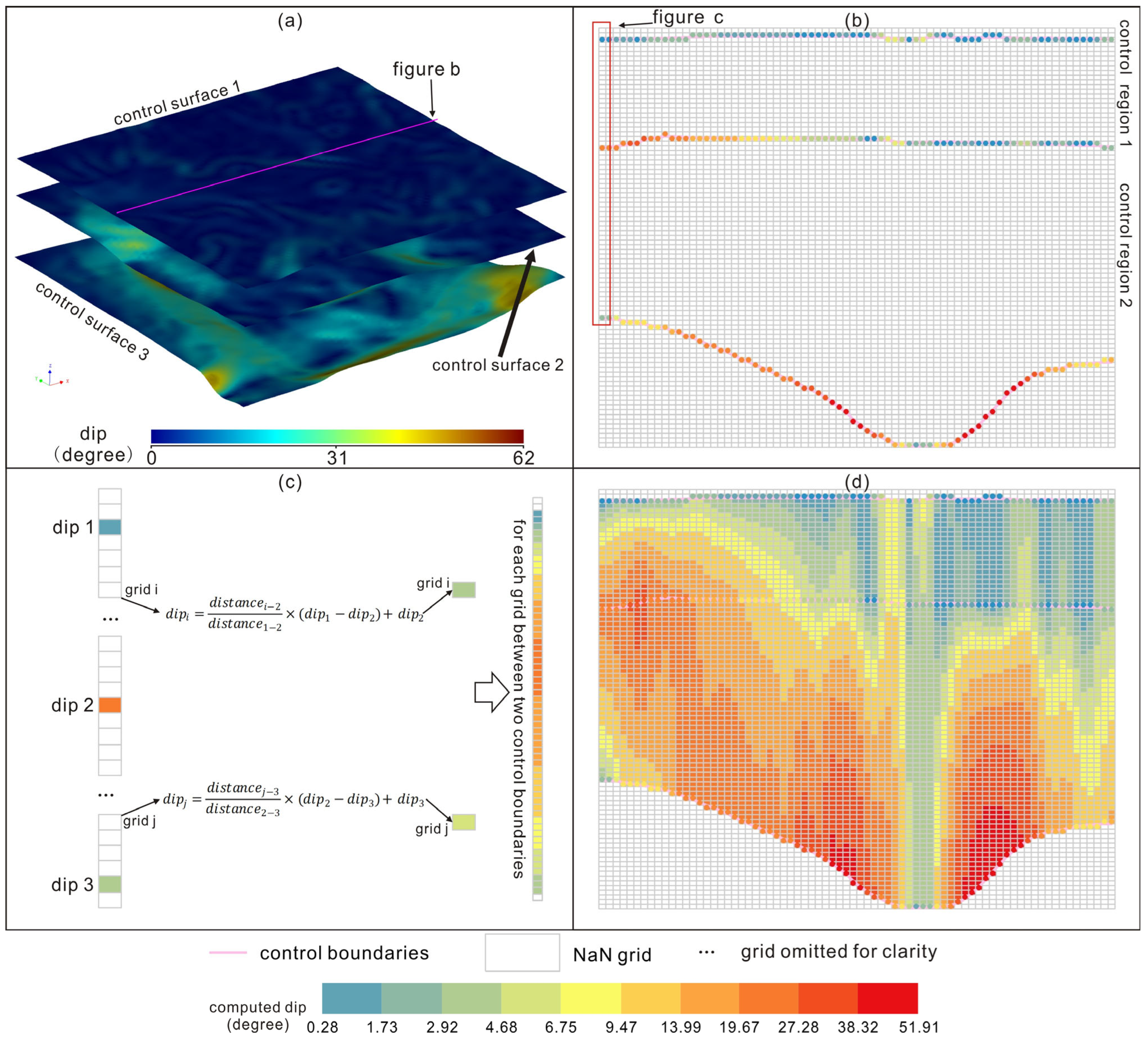
① Terrain interface construction and optimization: generating QLS top interfaces using DEMs and multi-source terrain data (Figure 3a); outputs are calibrated against modeling objectives by excluding micro-topographic features (e.g., small depressions and channel convexities/concavities) in regional-scale models; corrected strike, dip, and dip angles are extracted at all interface points.
② Control geological surface building: constructing base surface (line) from existing boundary data; deriving strike/dip/dip angle at any surface point (Figure 3a); and adding intermediate control surfaces where required (e.g., fluvial-influenced layers for local feature enhancement, Figure 3b,c).
③ Field variogram parameter calculation: sequentially extracting interfaces from the bottom to the top with the corresponding dip/strike; parameters are assigned to intersecting grids via adjacent interface weighted averaging; the aforementioned process is iteratively repeated until full parameterization of all target grids is achieved (Figure 3d).
(3) Determining valuation pathways for geostatistical simulation algorithms
In geostatistical simulation algorithms, the pathways chosen for simulation significantly impact modeling outcomes, a principle that also applies to the proposed method in this study. The gradual deposition of QLS toward accumulation zones follows a progression from near to far. Thus, the interpolation method that expands from current sampling points to distant locations is consistent with sedimentation principles. Conversely, QLS accumulates vertically from bottom to top. Therefore, when horizontal distances are equivalent, sequential interpolation from bottom to top should be applied to better matches the QLS deposition process.
Based on this understanding, the steps for determining valuation pathways are as follows:
① Assign discrete variable data (Figure 4a) to corresponding grids based on their spatial positions (Figure 4b).
② Extract grids within the effective range of QLS.
③ Traverse each grid to calculate the horizontal and vertical distances to the nearest valid data points.
④ If a current grid’s Z-coordinate exceeds the Z-value range of its nearest data point, then calculate the distance to the next data point (Figure 4c).
⑤ If this Z-value exceeds the Z-range of all data points, select the minimum distance corresponding to the farthest data point (Figure 4c).
⑥ Determine the valuation path in ascending order of the horizontal distance (Figure 4d).
⑦ When horizontal distances are equal, a single upward traversal (Figure 4e) is sufficient for evaluation.
(4) Ordered IK with field variogram parameters
Variogram parameters significantly impact the outcomes of Kriging interpolation. Dip angle and inclination values are embedded within each target grid node, which facilitates either real-time estimation during iterative processing or partition-based assessment using raw data. Using IK coupled with variogram analysis, we derive probability estimates for discrete variables at each grid position. The variable with the maximum probability is selected as the estimated value. This process is repeated until all nodes within the modeling domain have been estimated.
Computational acceleration is implemented via parallel estimation of nodes sharing identical horizontal distances to enhance algorithmic efficiency.
(5) Optimization and Application of Modeling Results
The modeling outcomes from the aforementioned steps may still contain isolated strata that were not processed through the modeling data. These could result from two factors: either thin strata with discontinuities caused by inclination effects, or minimal random variations introduced during sequential interpolation. These issues can be resolved through human–computer interaction or filtering techniques. After optimizing the valuation results, they can be applied to quantitative studies such as groundwater resource assessments and liquefaction potential analyses of sandy soils.

3. Case Studies

3.1. Simple 2D Lithology Profile Reconstruction

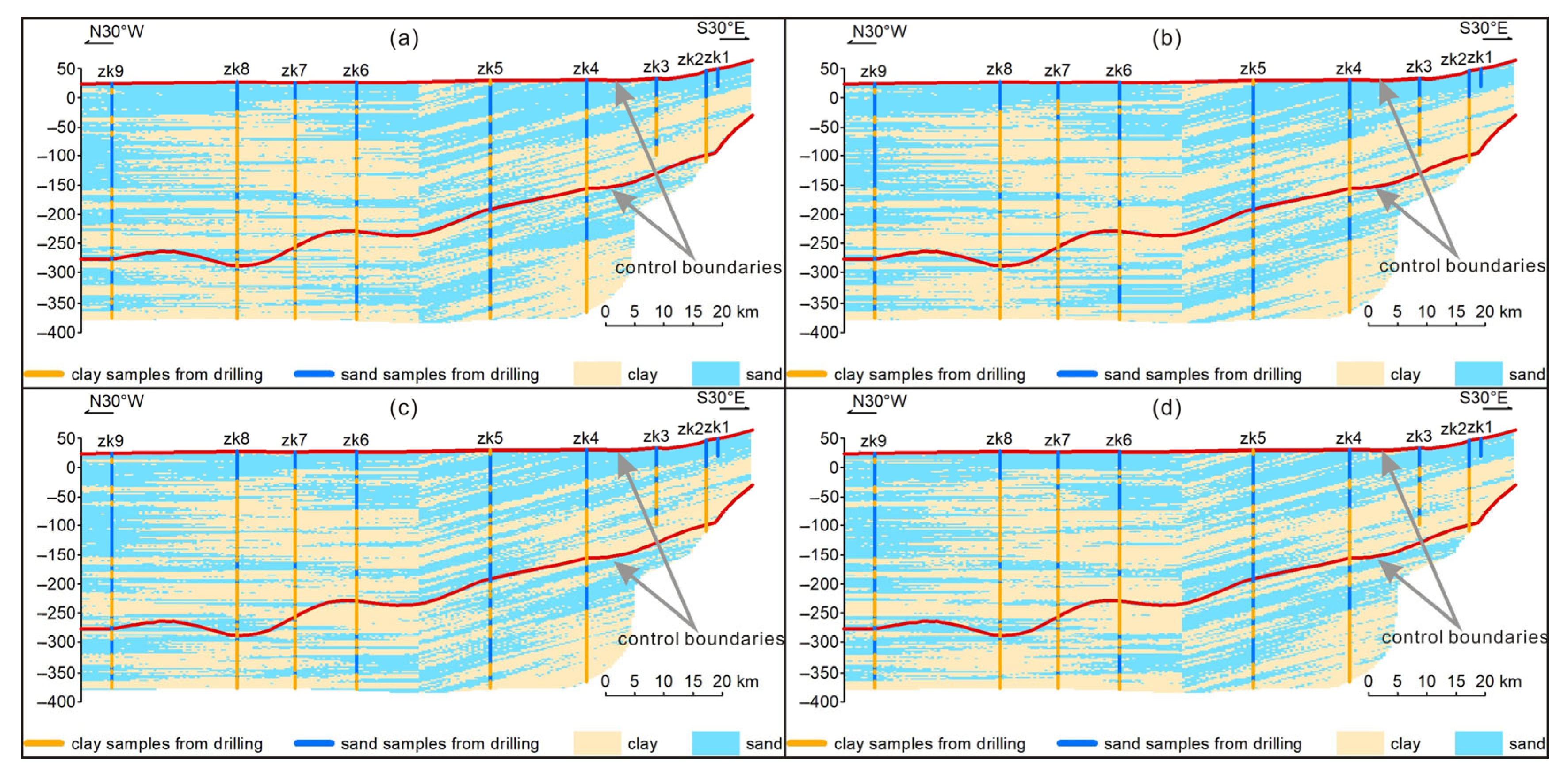
The primary objective for geologists is to estimate the spatial distribution of QLS lithology. Traditional studies often depict QLS distribution using cross-sectional profiles. This paper uses a typical hydrogeological profile situated in northwestern Shandong Province, China, as an example. The terrain is characterized by higher elevations in the southeast and lower elevations in the northwest. The southeastern section has relatively thin Quaternary strata that gradually thickens toward the northwest (Figure 5). In the adjacent mountainous areas, the QLS formation shows a significant northwestward inclination. The dip angle decreases from steep to nearly horizontal as the formation accumulates. During preliminary research, hydrogeological experts drilled nine boreholes, primarily dividing the QLS formation into clayey and sandy layers (which correspond to weakly permeable and water-bearing zones, respectively). The experts mapped the hydrogeological profile of the study area (Figure 5a) using their expertise. This map approximately reflects the gradual reduction process of the QLS formation inclination from steep to nearly horizontal. Furthermore, the hydrogeologists integrated Quaternary data and hydrogeological information to delineate the boundaries of the water-bearing zones in the study area (red line in Figure 5a). Considering the regional nature of this hydrogeological profile, the modeling team simplified the Quaternary boundary to minimize interference from local phenomena such as river channels or depressions.
Based on the aforementioned data, this study conducted dip angle and inclination calculations using the red boundary in Figure 5a. The study also determined the effective distance between the estimated grid and borehole data and performed ordered IK estimation. The results are shown in Figure 5b,c. The analysis reveals that the estimation outcomes largely replicate the spatial distribution pattern of QLS, aligning with the geological knowledge of hydrogeological experts. Notably, the results closely match the spatial variations of the control boundaries. Figure 5b tested the impact of a non-sequential valuation order during estimation. Figure 5c demonstrated the effect of adopting a sequential, bottom-up approach and showed minimal differences between the two methods. The former exhibited random effects due to the randomness inherent in the vertical sequence order, which mitigated the step-like effect of the IK method to some extent. Conversely, the latter showed reduced randomness but intensified step-like effects. Both methods revealed significant steepening effects at stratigraphic contact zones, which compromised the modeling results’ aesthetic appeal.
Furthermore, the SISIM model was developed to test the validity of the proposed approach. Traditional hydrogeological expertise suggests that QLS estimation in mountainous areas relies on the dip trend of the strata, whereas estimation in plain areas relies on the near-horizontal distribution trend. The QLS distribution trend between these two zones is intermediate and transitions gradually. From a modeling perspective, this study divides the area into two zones: the mountainous zone and the plain zone. Lithology distributions are simulated separately in each zone. The simulation results shown in Figure 6 illustrate this: the mountainous zones used a mean dip of 14.5°, while the plains adopted horizontal modelling. These results reveal considerable stochasticity, particularly in the form of distinct stratigraphic contact irregularities at the boundaries between zones. The results also show a distinct, sharp contact between the adjacent strata, particularly in the contact zone. One of the reasons is that the stratum inclination angle represents a gradual transition. However, the partitioned scheme can only approximate this transition state and cannot depict the change precisely, which results in unnatural contact between strata. Additionally, the significant difference in stratum thickness is another reason for the steep contact. Although SISIM allows the integration of geological principles, it is challenging to accommodate the complex constraints inherent in the proposed method.
A comparative analysis of the proposed method and expert-derived interpretations reveals significant discrepancies in QLS characterization. For instance, the former shows fluctuations in QLS inclination within the zk6–8 borehole range, whereas the latter shows nearly horizontal patterns. Regarding the genesis of the QLS, the modelling results from this method seem more credible if the optimal control boundary at the base indicates sedimentary topography during deposition, as they reflect the significant influence of terrain on the QLS. Furthermore, expert profiles demonstrate significant subjectivity when connecting borehole strata, with substantial variations in mapping outcomes among different experts, highlighting the limitations of expert knowledge. Overall, the proposed method can effectively reproduce the spatial distribution of QLS to a certain extent.

3.2. Complex 2D Lithology Profile Building

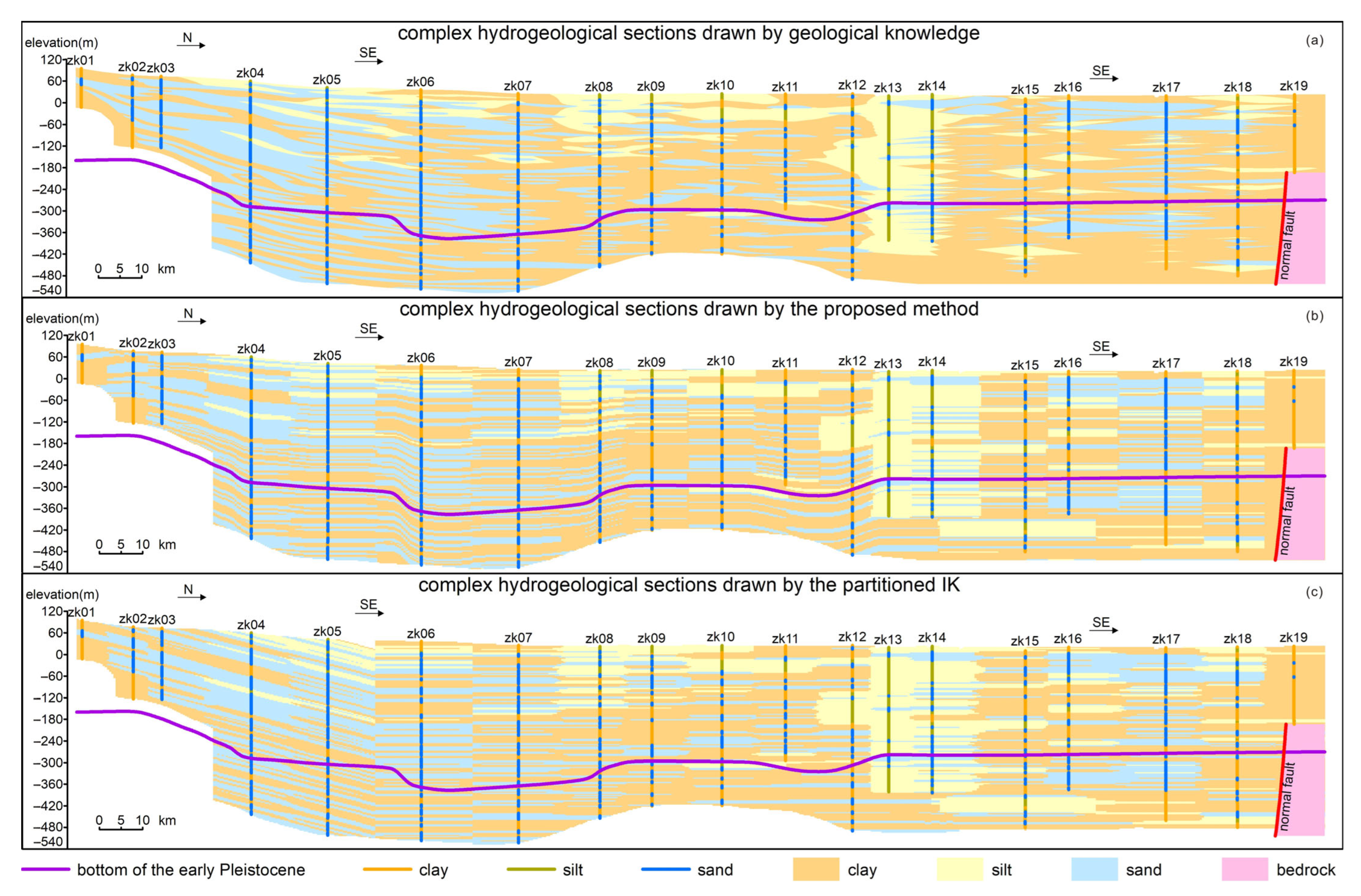
Reconstructing QLS formations under complex geological conditions continues to remain a significant challenge. This study validates the proposed methodology by using a hydrogeological profile that spans the North China Plain as a case study. The profile traverses two river basins, the Haihe and Yellow Rivers, and extends 280 km from northwest to southeast [44]. The terrain descends from an elevation of approximately 100 m A.S.L. in the northwest to around 30 m A.S.L. in the southeast. Previously, hydrogeologists classified QLS lithology into three categories: clay, silt/silty clay, and sandy soil. Using stratigraphic data from 19 boreholes, the hydrogeologists developed an expert knowledge profile (Figure 7a). The modeling team systematically compiled Quaternary boundary information and delineated the Early Pleistocene basement boundary (purple line) depicted in the figure. They extended this boundary along the right side of the fault zone to define the distribution of QLS formations. Additionally, geologists observed that the Minghua Town Formation is incompletely consolidated, suggesting that the basement boundary’s dip angle could control spatial distribution patterns.
Figure 7b illustrates modeling results of the proposed method, which approximately reproduces the spatial distribution of QLS along the profile. The expert knowledge profiles on the left side of zk6 account for the dip state of the strata; the remaining sections predominantly follow the near-horizontal principle of QLS. In contrast, our method incorporates local stratigraphic dips at locations such as zk08 and zk12. This approach better aligns with complex and variable sedimentary environments. The difference likely stems from experts’ tendency to prioritize topographic factors when data is scarce. Additionally, the subjective nature of connecting adjacent boreholes in expert profiles reflects both the richness of geological understanding as well as the incomplete interpretation of stratigraphic distribution patterns under sparse data. The proposed method’s modeling results comprehensively consider the combined effects of top-to-bottom interface morphology, thereby reducing subjectivity in profile mapping.
This study utilized the partitioned IK method to determine the QLS distribution profile (Figure 7c). The inclination angles at zk01 through zk05 are 14.89°, while zk06 exhibits a dip angle of 4.5° with a 0° dip on the right. The results show flat stratigraphic dips between zones and unnatural contact interfaces with distinct step-like effects. The evaluation process is notably similar to mechanical computer operations, lacking geological constraints, leading to discrepancies from expert knowledge. While gradually increasing zone density could mitigate this issue, significant vertical variations in stratigraphic dips further complicate interpolation tasks further, deterring geologists from adopting the IK method.
Compared to other approaches, our method exhibits superior spatial variation characteristics, but it also shows noticeable, step-like modeling patterns that are more pronounced than those of partitioned IK. Analysis reveals that this stems from assigning values to adjacent zones after determining the evaluation path. Despite incorporating more geological knowledge, our method still deviates from expert profiles. If we conduct optimizations of human–computer interaction, our method may surpass both approaches. This enhances the spatial representation capabilities of QLS and advances the application of geological statistics in modern detailed geological surveys.

3.3. Complex 3D Lithological Model Reproduce

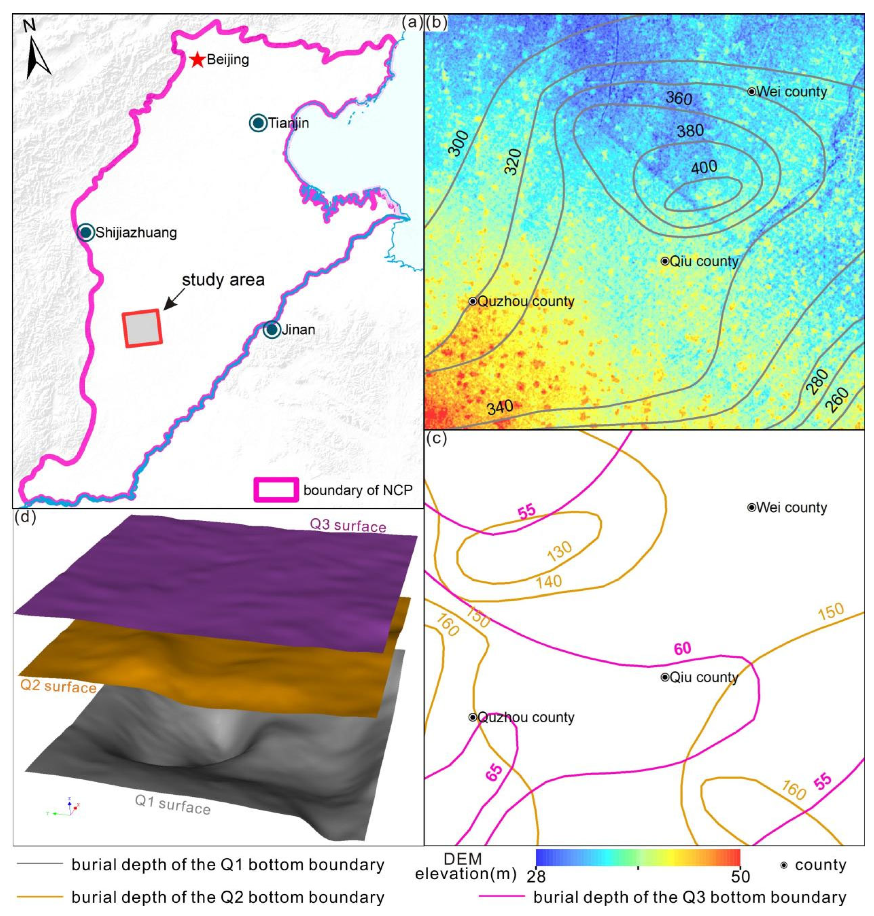
Geological bodies are 3D entities. Due to data scarcity and technical constraints [45], the representation of geological information using points, lines, and surfaces has been a reluctant choice. However, the rapid advancement of 3D geological modeling technology has made detailed 3D model construction increasingly popular among geological experts. Nevertheless, creating complex geological models within the confines of current technology remains a significant challenge. This study selected a complex research area located in the central-western part of the North China Plain (Figure 8a) to test the stability and reliability of the proposed method. The study area is entirely situated on an alluvial plain. Only the northwestern part of Quzhou County forms the front edge of the Shahe and Luohe alluvial fans. The terrain is higher in the southwest and lower in the northeast, featuring a relatively flat topography. Geologists conducted systematic research on the study area [44] and divided the QLS, within a 400 m burial depth, into four periods: Q1, Q2, Q3, and Q4. They also mapped depth contour lines for each period’s stratigraphic interfaces (Figure 8b,c). Previous studies drilled 51 boreholes, only 10 of which exposed the Q1 base boundary. Figure 9b shows the lithology distribution of these boreholes. Shallow QLS sediments exhibit approximate horizontality, and the Q3 interface is relatively flat. Many shallow boreholes either failed to obtain cores or yielded coarse core samples. Therefore, this study focuses on modeling the Q1 and Q2 strata. Figure 8d illustrates the three stratigraphic interfaces involved, where the morphological variations at the Q1 base boundary better validate the robustness of the proposed method.
After completing the valuation path evaluation and assigning the inclination angles, the ordered IK valuation results are depicted in Figure 9. This figure represents the combined outcomes of the independent Q1 and Q2 estimations. Figure 9a,b show that the model accurately reproduces the distribution pattern of QLS with minimal simplification of the raw data. To illustrate changes in QLS sedimentation trends, clay and sandy strata were extracted within 50 m above the Q1 base boundary and 50 m above and below the Q2 boundary. Figure 8c,d illustrate the spatial distributions of these layers. Elevation variations show that he morphology of the Q1 base boundary influences both clay and sandy strata, extending along the sedimentary base boundary toward surrounding areas. At the depression in the central Q1 formation, particularly, the vertical trend aligns with QLS sedimentation patterns under similar depositional conditions. This becomes more apparent in the cross-sectional view in Figure 9g. Figure 9e,f,h show comparable distribution patterns of QLS strata within Q2. However, the proposed method still exhibits a distinct step-like effect when estimating QLS strata, which indicates the need for further research.
According to hydrogeological experts, the strata in the study area will be examined for spatial distribution in a roughly horizontal manner. We used the IK method to create a lithological distribution model within ±50 m of Q1 and ±50 m of Q2. The variogram function ranges are 200 m × 200 m × 3 m, and the results are shown in Figure 10. The modeling results indicate that the continuity between strata has deteriorated, and most strata are distributed horizontally. This aligns with the traditional understanding of hydrogeology. Additionally, a relatively obvious step effect is present in the lithology distribution. Inestimable phenomena in the modeling space reduce the valuation effect to some extent. A comparison of the two results reveals that the proposed method exhibits stronger stratigraphic continuity and aligns with the understanding of stratigraphic era changes. This suggests that the proposed method may offer a more accurate representation of the actual situation. However, the lithological distribution constructed by the traditional method aligns with the hydrogeological understanding; it may still deviate from the actual situation due to sparse data. Both estimation results show an obvious step effect that needs to be studied and resolved in future research.

4. Discussion

4.1. The Advantages of the Proposed Method

Through three case studies, the proposed methodology effectively integrates expert knowledge into modelling processes. The resulting models and their evolutionary trends better align with sedimentary principles, enhancing the efficiency with which geologists can reconstruct QLS stratigraphic distributions while incorporating geological insights to minimise discrepancies between simulations and actual conditions. The hydrogeology expert can refine the distribution of discrete variables in QLS and extract the aquifer group from the modelling results. This approach also enhances the application of traditional geological statistics in geological reconstruction.
Hydrogeologists cannot determine aquifer conditions anywhere. It is unreasonable to test the reliability of modeling results by extracting boreholes or sample points in regional geological modeling. Instead, modeling experts typically verify the reliability of results by comparing them with their own knowledge and achievements. To evaluate differences between modeling results and expert-defined sections, this study calculated errors in relation to reference profiles derived from various grid-to-expert-profile area ratios, using case 2 as an example. The error metrics were 26.3% for partitioned IK and 27.8% for the proposed method. There are two potential causes of these errors: the natural transition of QLS in expert interpretations, and the timing mismatches between age boundary mapping and profile compilation. Although partitioned IK aligns better with expert references, its structural forms do not meet hydrogeological standards. Conversely, our method effectively captures QLS spatial patterns in complex depositional settings. We believe that the modeling results of the proposed method more accurately reflect the actual geological conditions than those of the partitioned IK method.

4.2. The Limit of the Proposed Method

However, challenges remain in the following two aspects. The first one is a distinct step-like stratigraphic pattern; it greatly affects the aesthetic appeal and acceptability of the modeling results. This is because geological experts prefer a more natural form of contact between strata. This phenomenon is primarily caused by the large thickness of the strata and the almost identical weight competition process between sample points on either side. In other words, the sequential valuation order of the points to be estimated in the middle of the samples makes the distances and quantities of the samples approximately the same, causing the strata to contact each other in a nearly vertical manner. When the difference in stratum thickness is small, this effect is weakened to a certain extent. However, when the difference in stratum thickness is large, it is difficult to offset the significant weight difference. This problem can be solved by human–machine interaction in actual application. The second issue is the high reliance on expert estimation for interpolating trends. For example, the strata in the plain area are regarded as being distributed near-horizontally, but if the control boundaries are inclined in the modelling process, the strata will be modelled as being correspondingly inclined. This modelling result may better align with the actual geological situation, so the control boundaries need to be specified carefully before modelling the QLS distribution.
Further research is required to achieve more complex geological condition reconstructions. Furthermore, as experts develop a comprehensive understanding of sedimentary evolution mechanisms, incorporating dynamic geological constraints into modelling will facilitate broader applicability across various geological scenarios, particularly bedrock strata.

5. Conclusions

Precise reconstruction of the spatial distribution of QLS remains a significant challenge. This study uses the ordered IK estimation method, based on Kriging theory, to investigate complex and variable QLS formations. Firstly, the method digitizes expert knowledge data to obtain dip and strike information for target points. Then it calculates the distance between estimated values and actual data to determine evaluation paths. Finally, it performs IK valuations along these paths, expanding QLS discrete variable distributions from near to far in a data-centric manner.
Three distinct study areas were analyzed from 2D and 3D perspectives to validate the method’s feasibility and robustness. The results demonstrate its alignment with expert perceptions and improved accuracy compared to traditional methods, while requiring minimal simplification of element data. This makes the method suitable for reconstructing complex geological conditions. Nevertheless, hydrogeological experts may still need a certain level of human–machine interaction to achieve smooth, high-quality interpolation results, representing a significant improvement in efficiency over manual drawing.
Besides, improvements are needed in step effect processing, visual presentation, and computational efficiency for future research. Additionally, the mathematical basis and optimization scheme of the proposed method must be addressed.
Overall, this method incorporates more expert knowledge into the valuation process, improving QLS distribution reconstruction to some extent. When combined with expert insights, it produces superior results to those of conventional approaches. This method provides efficient, high-quality solutions for estimating QLS discrete variables in complex regions beyond hydrogeological modeling, such as engineering geological modeling or Quaternary strata modeling. Thus, it advances the application of geostatistics in various geological fields.

Author Contributions

G.J.: Conceptualization, Investigation, Methodology, Visualization, Writing—original draft; Z.C.: Funding acquisition, Validation, Methodology; K.X.: Conceptualization, Methodology, Methodology, Supervision, Writing—review and editing; Y.L.: Conceptualization, Methodology, Funding acquisition, Visualization; Q.W.: Conceptualization, Investigation, Data curation. All authors have read and agreed to the published version of the manuscript.

Funding

This research was supported by the Geological Exploration Fund Project of the Department of Natural Resources of Shandong Province (Grant No. LU KAN ZI (2024) 72), the China Geological Survey Program (Grant Nos. DD20230719, DD20230427) and the Fundamental Research Funds for Central Public Welfare Research Institutes, CAGS (Grant No. SK202410).

Data Availability Statement

The raw data supporting the conclusions of this article will be made available by the authors on request.

Conflicts of Interest

The authors declare no conflicts of interest.

References

  1. Qiao, X.; Cheng, T.; Zhang, L.; Sun, N.; Ding, Z.; Shi, Z.; Wang, G.; Zhang, Z. Zoning Method for Groundwater Pollution Risk Control in Typical Industrial–Urban Integration Areas in the Middle Reaches of the Yangtze River. Water 2025, 17, 2249. [Google Scholar] [CrossRef]
  2. Zhang, J.; Liesch, T.; Goldscheider, N. Impacts of climate change and human activities on global groundwater storage from 2003 to 2022. J. Hydrol. 2025, 664, 134298. [Google Scholar] [CrossRef]
  3. Crayol, E.; Huneau, F.; Garel, E.; Zuffianò, L.E.; Limoni, P.P.; Romanazzi, A.; Mattei, A.; Re, V.; Knoeller, K.; Polemio, M. Investigating pollution input to coastal groundwater-dependent ecosystems in dry Mediterranean agricultural regions. Sci. Total Environ. 2024, 954, 176015. [Google Scholar] [CrossRef]
  4. Zhai, Y.; Jiang, Y.; Cao, X.; Leng, S.; Wang, J. Valuation of ecosystem damage induced by soil-groundwater pollution in an arid climate area: Framework, method and case study. Environ. Res. 2022, 211, 113013. [Google Scholar] [CrossRef] [PubMed]
  5. Zhang, J.; Xuan, Y.; Lei, J.; Bai, L.; Zhou, G.; Mao, Y.; Gong, P.; Zhang, M.; Pan, D. Heavy metals prediction system in groundwater using online sensor and machine learning for water management: The case of typical industrial park. Environ. Pollut. 2025, 374, 126270. [Google Scholar] [CrossRef]
  6. Kumar, D.; Kumar, G.; Kumari, A. High resolution geophysical and geospatial mapping of quaternary sediments for exploration and assessment of groundwater in Ghaziabad district, Uttar Pradesh, India. Groundw. Sustain. Dev. 2021, 14, 100638. [Google Scholar] [CrossRef]
  7. Shen, S.; Luo, K.; Ma, T.; Du, Y.; Liang, X.; Zhang, J.; Han, Z.; Ye, X. Nitrogen burial characteristics of Quaternary sediments and its controls on high ammonium groundwater in the Central Yangtze River Basin. Sci. Total Environ. 2022, 842, 156659. [Google Scholar] [CrossRef]
  8. Zhao, H.; Wei, W.; Liu, J. Review of application of high-resolution sequence stratigraphy in Quaternary aquifer division. Adv. Sci. Technol. Water Resour. 2016, 36, 88–94. [Google Scholar]
  9. Journel, A.G.; Isaaks, E.H. Conditional Indicator Simulation: Application to a Saskatchewan uranium deposit. J. Int. Assoc. Math. Geol. 1984, 16, 685–718. [Google Scholar] [CrossRef]
  10. Mallet, J.L. Discrete smooth interpolation in geometric modelling. Comput.-Aided Des. 1992, 24, 178–191. [Google Scholar] [CrossRef]
  11. Nalder, I.A.; Wein, R.W. Spatial interpolation of climatic Normals: Test of a new method in the Canadian boreal forest. Agric. For. Meteorol. 1998, 92, 211–225. [Google Scholar] [CrossRef]
  12. Boumpoulis, V.; Michalopoulou, M.; Depountis, N. Comparison between different spatial interpolation methods for the development of sediment distribution maps in coastal areas. Earth Sci. Inform. 2023, 16, 2069–2087. [Google Scholar] [CrossRef]
  13. Ji, G.; Cai, Z.; Tan, X.; Wang, T.; Wang, C.; Xu, Q.; Zhou, B.; Cui, Y. Refined construction of semi-provincial hydrogeological models using hierarchical modeling: A case study in Western Shandong Province, China. J. Hydrol. Reg. Stud. 2025, 58, 102222. [Google Scholar] [CrossRef]
  14. Ji, G.; Wang, Q.; Zhou, X.; Cai, Z.; Zhu, J.; Lu, Y. An automated method to build 3D multi-scale geological models for engineering sedimentary layers with stratum lenses. Eng. Geol. 2023, 317, 107077. [Google Scholar] [CrossRef]
  15. Al-Mudhafar, W.J. Bayesian kriging for reproducing reservoir heterogeneity in a tidal depositional environment of a sandstone formation. J. Appl. Geophys. 2019, 160, 84–102. [Google Scholar] [CrossRef]
  16. Li, Z.; Zhang, X.; Zhu, R.; Clarke, K.C.; Weng, Z.; Zhang, Z. Direct kriging: A direct optimization based model with locally varying anisotropy. J. Hydrol. 2024, 639, 131553. [Google Scholar] [CrossRef]
  17. Deal, P.T.; Sabatini, D.A. Utilizing indicator kriging to identify suitable zones for manual drilling in weathered crystalline basement aquifers. Groundw. Sustain. Dev. 2020, 11, 100402. [Google Scholar] [CrossRef]
  18. Hidalgo-Arellano, I.; Fernández-Avilés, G. Spatial depopulation risk assessment through spatial principal component analysis and indicator kriging in Castilla-La Mancha (Spain). J. Rural Stud. 2025, 119, 103771. [Google Scholar] [CrossRef]
  19. Carr, J.R.; Mao, N. A general form of probability kriging for estimation of the indicator and uniform transforms. Math. Geol. 1993, 25, 425–438. [Google Scholar] [CrossRef]
  20. Rendu, J. Disjunctive kriging: Comparison of theory with actual results. J. Int. Assoc. Math. Geol. 1980, 12, 305–320. [Google Scholar] [CrossRef]
  21. Tolosana-Delgado, R.; Pawlowsky-Glahn, V.; Egozcue, J.J. Simplicial Indicator Kriging. J. China Univ. Geosci. 2008, 19, 65–71. [Google Scholar] [CrossRef]
  22. Yang, S.; Hou, W.; Chen, Y.; Li, Y.; Ye, S. Three-dimensional reconstruction of geologic structures based on adaptive fully-connected deep neural network and multi-point statistics method. Earth Sci. Front. 2025, Online, 1–25. [Google Scholar]
  23. Zhao, Z.; Zhang, L.; Bi, E. Spatial interpolation of highly skewed data of the Junggar Basin phreatic groundwater through the multi-scale cokriging model. Earth Sci. Inform. 2022, 15, 1737–1748. [Google Scholar] [CrossRef]
  24. Zhang, W.; Duan, T.; Liu, Y.; Wang, M.; Lian, P.; Zhao, L. Application Status and Development Trend of Quantitative Geological Modeling. Geol. Sci. Technol. Inf. 2019, 38, 264–275. [Google Scholar]
  25. Hou, W.; Chen, Y.; Liu, H.; Xiao, F.; Liu, C.; Wang, D. Reconstructing Three-dimensional geological structures by the Multiple-point statistics method coupled with a deep neural network: A case study of a metro station in Guangzhou, China. Tunn. Undergr. Space Technol. 2023, 136, 105089. [Google Scholar] [CrossRef]
  26. Park, E. 3D nonstationary lithofacies characterization via manifold embedding and transition probabilities for hydrogeological applications. J. Hydrol. 2025, 660, 133453. [Google Scholar] [CrossRef]
  27. Hou, W.; Liu, H.; Zheng, T.; Chang, H.; Xiao, F. Extended GOSIM: MPS-Driven Simulation of 3D Geological Structure Using 2D Cross-Sections. Earth Space Sci. 2022, 9, e2021EA001801. [Google Scholar] [CrossRef]
  28. Ye, S.; Hou, W.; Yang, J.; Wang, H.; Bai, Y. Advance of 3D smart geological modeling. Earth Sci. Front. 2025, 32, 182–198. [Google Scholar]
  29. Chen, Q.; Cui, Z.; Liu, G.; Yang, Z.; Ma, X. Deep convolutional generative adversarial networks for modeling complex hydrological structures in Monte-Carlo simulation. J. Hydrol. 2022, 610, 127970. [Google Scholar] [CrossRef]
  30. Cui, Z.; Chen, Q.; Liu, G. A two-stage downscaling hydrological modeling approach via convolutional conditional neural process and geostatistical bias correction. J. Hydrol. 2023, 620, 129498. [Google Scholar] [CrossRef]
  31. Lyu, B.; Wang, Y.; Shi, C. Multi-scale generative adversarial networks (GAN) for generation of three-dimensional subsurface geological models from limited boreholes and prior geological knowledge. Comput. Geotech. 2024, 170, 106336. [Google Scholar] [CrossRef]
  32. Song, S.; Mukerji, T.; Hou, J.; Zhang, D.; Lyu, X. GANSim-3D for Conditional Geomodeling: Theory and Field Application. Water Resour. Res. 2022, 58, e2021WR031865. [Google Scholar] [CrossRef]
  33. Sun, C.; Demyanov, V.; Arnold, D. A conditional GAN-based approach to build 3D facies models sequentially upwards. Comput. Geosci. 2023, 181, 105460. [Google Scholar] [CrossRef]
  34. Yang, Z.; Chen, Q.; Cui, Z.; Liu, G.; Dong, S.; Tian, Y. Automatic reconstruction method of 3D geological models based on deep convolutional generative adversarial networks. Comput. Geosci. 2022, 26, 1135–1150. [Google Scholar] [CrossRef]
  35. Keegan-Treloar, R.; Werner, A.D.; Irvine, D.J.; Banks, E.W. Application of Indicator Kriging to hydraulic head data to test alternative conceptual models for spring source aquifers. J. Hydrol. 2021, 601, 126808. [Google Scholar] [CrossRef]
  36. Journel, A.G. Nonparametric estimation of spatial distributions. J. Int. Assoc. Math. Geol. 1983, 15, 445–468. [Google Scholar] [CrossRef]
  37. Masoudi, M.J.; Ashrafzadeh, A.; Khaledian, M.; Janatrostami, S. Assessment of groundwater quality for agricultural purposes in Qazvin Province, northwestern Iran: A fuzzy inference and indicator Kriging approach. Environ. Sustain. Indic. 2024, 24, 100528. [Google Scholar] [CrossRef]
  38. Baccou, J.; Liandrat, J. Kriging-based subdivision schemes: Application to the reconstruction of non-regular environmental data. Math. Comput. Simul. 2011, 81, 2033–2050. [Google Scholar] [CrossRef]
  39. Xiao, N.; Guo, J.; Kuang, Z.; Wang, W. Application of data partitioned Kriging algorithm with GPU acceleration in real-time and refined reconstruction of three-dimensional radiation fields. Ann. Nucl. Energy 2025, 212, 111047. [Google Scholar] [CrossRef]
  40. Chen, Q.; Liu, G.; Ma, X.; Li, X.; He, Z. 3D stochastic modeling framework for Quaternary sediments using multiple-point statistics: A case study in Minjiang Estuary area, southeast China. Comput. Geosci. 2020, 136, 104404. [Google Scholar] [CrossRef]
  41. Tian, M.; Cheng, J. Quaternary Geology and Geomorphology; Geology Press: Beijing, China, 2009; p. 310. [Google Scholar]
  42. Nichols, G. Sedimentology and Stratigraphy, 2nd ed.; Wiley-Blackwell: Oxford, UK, 2009; p. 412. [Google Scholar]
  43. Montero, J.M.; Fernández-Avilés, G.; Mateu, J. Spatial and Spatio-Temporal Geostatistical Modeling and Kriging; Wiley: Chichester, UK, 2015; p. 400. [Google Scholar]
  44. Zhang, Z.; Fei, Y. Atlas of Groundwater Sustainable Utilization in North China Plain; Sinomap Press: Beijing, China, 2009; p. 53. [Google Scholar]
  45. Zhu, J.; Gan, T.; Liu, S.; Zhou, X.; Zhang, L.; Huo, Z. 3D Hydrogeological Structure Modeling Based on Quantitative Correlation and Identification of Aquifer Types Within Stratigraphic Layers. Water 2024, 16, 3271. [Google Scholar] [CrossRef]
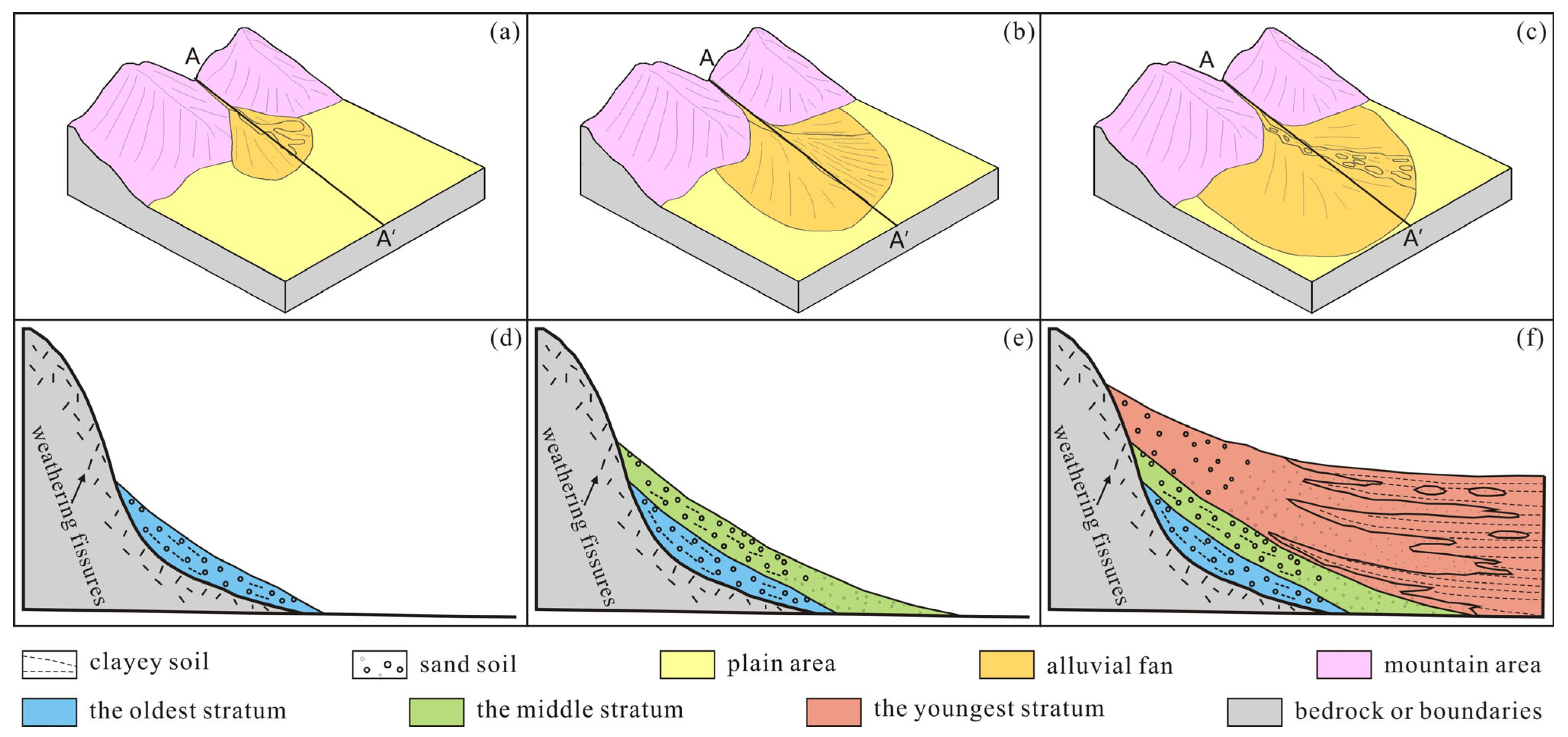
Figure 1. The diagram roughly illustrates the depositional processes of alluvial fan formation (modified from [42]). (a) presents the conceptual framework, while (d) displays the corresponding cross-sectional profile, both illustrating the initial developmental stage of the alluvial fan. Similarly, (b,e) depict the intermediate stage, (c,f) show the mature stage.
Water 17 03116 g001
Figure 2. A comparison of the search strategies of the different methods: (a) traditional partitioned IK and (b) our proposed ordered IK with field variogram parameters. Note that the arrow with parameters indicates the primary direction during IK interpolation. The figure depicts only five sub-regions between adjacent drill points, whereas each grid or point-to-be-estimated corresponds to one sub-region.
Water 17 03116 g002
Figure 3. The flowchart illustrates the main workflow for calculating the dip at target estimation points. (a) Calculate the inclination and dip angle at any given point on the control interface, (b) mapped dip in section view, (c) computational method for determining dips in unassigned grid, (d) the distribution of dip angle in geological space.
Water 17 03116 g003
Figure 4. The general workflow of the ordered IK method with field variogram parameters. (a) original data and subdivided grids, (b) assigning the lithology values of the boreholes to the grid, (c) calculating the areal distance to the drill trajectory, (d) the interpolation order in the areal direction, (e) the interpolation order in the vertical direction with the same areal distance, (f) the interpolation result of the proposed method.
Water 17 03116 g004
Figure 5. Method comparison for complex hydrogeological section modeling: (a) manual geological interpretation, (b) proposed method without vertical interpolation order, (c) proposed method with vertical interpolation order.
Water 17 03116 g005
Figure 6. The four randomly selected modeling results of SISIM. (ad) present the four simulation results, respectively.
Water 17 03116 g006
Figure 7. A comparison of a complex hydrogeological section drawn by different methods. (a) hydrogeological section drawn by geologist, (b) modeling result by the proposed method, and (c) modeling results by the partitioned IK method.
Water 17 03116 g007
Figure 8. Location of the study area and data distribution map: (a) location of the study area in the NCP; (b) digital elevation model and burial depth of the Q1 bottom boundary; (c) burial depths of the Q2 (purple line) and Q3 (brown line) bottom boundaries; (d) geological surfaces of the Q1, Q2, and Q3 bottoms.
Water 17 03116 g008
Figure 9. The 3D modeling results of the study area obtained using the proposed method (vertical exaggeration = 0.5): (a) macro view; (b) micro view; (c) vertical clay distribution within + 50 m of the Q1 bottom; (d) vertical sand distribution within +50 m of the Q1 bottom; (e) vertical clay distribution within ±50 m of the Q2 bottom; (f) vertical sand distribution within ±50 m of the Q2 bottom; (g) lithological distribution of Q1 at cross-section J = 52; (h) lithological distribution of Q2 at cross-section J = 0. Note that elevations in sub-figures (cf) illustrate the sedimentary trend of the QLS formation.
Water 17 03116 g009
Figure 10. The 3D modeling results of the study area obtained using the conventional IK method (vertical exaggeration = 0.5): (a) lithological distribution within +50 m of the Q1 bottom in 3D; (b) lithological distribution within ±50 m of the Q2 bottom in 3D; (c) lithological distribution within +50 m of Q1 at cross-section J = 52; (d) lithological distribution within ±50 m of Q2 at cross-section J = 0. Note that the elevations in sub-figures (a,b) are the same as in Figure 9.
Water 17 03116 g010
Table 1. Advantages and disadvantages of commonly used interpolation/simulation methods.
MethodAdvantagesDisadvantages
IDWSimple to implement, highly effective, and capable of setting barriers.It is sensitive to data and has a distinct bull’s-eye shape. It is isotropic in the modeling process.
RBF [14]Its form is simple, independent of dimensions, and requires minimal calculation.It has strict data requirements, and the quantity of input data significantly impacts computational efficiency. Inconsistent data distribution reduces computational efficiency, and increasing data slows down the speed.
DSI [10]It produces smooth and continuous interpolation results and can handle irregular geometric shapes.It has high computational complexity and difficulty capturing local features in highly heterogeneous regions.
Kriging-based methods [12,23]It provides optimal and linear unbiased estimation, is capable of evaluating uncertainties, is highly adaptable, and considers spatial autocorrelation.The computational complexity is high, and the data must meet second-order stationarity and intrinsic assumptions. The data must also conform to a normal distribution.
IK [17,18]There are no data distribution requirements, the valuation results are highly accurate, and soft data and both discrete and continuous variables can be used.When the threshold value is close to the sampling value, the accuracy near the threshold is low. The results of adding or deleting data points are unstable and exhibit a significant step-like effect. Its result has pronounced step effects. Probability estimation results may exceed [0, 1] bounds
SISIM [24]There is no requirement for data assumptions. Soft data can be used. It can simulate anisotropic geological phenomena.The computational load is high, the target shape is not expressed well, and the variogram function cannot be accurately restored.
MPS [25,26,27]It can better reproduce the geometric shapes of geological bodies. The characterization of river and alluvial fan sand bodies is excellent, and it is highly flexible and scalable.Training images must be stable and highly representative. The simulation of complex targets still has room for improvement, as it has a high computational load and is not very efficient. It suffers from embedded model dependency and local continuity artifacts.
ML-based method [28]It has improved modeling efficiency to some extent, reduced the amount of human–computer interaction, and possesses a certain learning ability. It has also enhanced modeling accuracy to a certain extent.Reconstructing complex geological conditions is still difficult. Large-scale and high-dimensional data are computationally inefficient, the training effect is poor, and the extracted geological features are limited.
DL-based method [22,29,30,31,32,33,34]The multi-layer neural network architecture can automatically extract features, model nonlinearly, and map high-dimensional data. These capabilities effectively improve modeling accuracy and reduce the need for human intervention.Fusing multimodal data is difficult. Black box models are difficult to integrate into geological cognition. They have high computational complexity, are challenging to train across dimensions, require large amounts of data, and lack dynamic update capabilities.
Disclaimer/Publisher’s Note: The statements, opinions and data contained in all publications are solely those of the individual author(s) and contributor(s) and not of MDPI and/or the editor(s). MDPI and/or the editor(s) disclaim responsibility for any injury to people or property resulting from any ideas, methods, instructions or products referred to in the content.